Abstract

Stochastic gradient-based optimization for discrete latent variable models is challenging due to the high variance of gradients. We introduce a variance reduction technique for score function estimators that makes use of double control variates. These control variates act on top of a main control variate, and try to further reduce the variance of the overall estimator. We develop a double control variate for the REINFORCE leave-one-out estimator using Taylor expansions. For training discrete latent variable models, such as variational autoencoders with binary latent variables, our approach adds no extra computational cost compared to standard training with the REINFORCE leave-one-out estimator. We apply our method to challenging high-dimensional toy examples and for training variational autoencoders with binary latent variables. We show that our estimator can have lower variance compared to other state-of-the-art estimators.

1 INTRODUCTION

Several problems in machine learning, such as variational inference and reinforcement learning, require the optimization of an intractable expectation of an objective function under a distribution with tunable parameters. Since exact gradients with respect to the parameters of the distribution are intractable, optimization must rely on unbiased stochastic estimates. Pathwise or reparametrization gradients (Glasserman,, 2003) have been shown to be effective for machine learning problems (Kingma and Welling,, 2014; Rezende et al.,, 2014; Titsias and Lázaro-Gredilla,, 2014), but they are only applicable to continuous distributions. A more general class of gradient estimators based on the score function method or REINFORCE (Glynn,, 1990; Williams,, 1992) is applicable to both continuous and discrete distributions. However, score function estimators suffer from high variance and reducing the variance remains an important open problem.

Variance reduction techniques for REINFORCE estimators range from simple baselines (Ranganath et al.,, 2014; Mnih and Gregor,, 2014) and Rao-blackwellization (Titsias and Lázaro-Gredilla,, 2015; Tokui and Sato,, 2017) to more advanced gradient-based control variates (Tucker et al.,, 2017; Grathwohl et al.,, 2018; Gu et al.,, 2016) and coupled sampling (Yin and Zhou,, 2019; Dong et al.,, 2020; Yin et al.,, 2020; Dimitriev and Zhou,, 2021). Another variance reduction method that has become prominent recently is the REINFORCE leave-one-out estimator (Salimans and Knowles,, 2014; Kool et al.,, 2019; Richter et al.,, 2020), that assumes $K\geq 2$ samples and uses a leave-one-out procedure to define sample-specific stochastic control variates. Despite its simplicity, this estimator performs very strongly for training discrete latent variables models (Dong et al.,, 2020; Richter et al.,, 2020; Dong et al.,, 2021). Presumably this is because the leave-one-out stochastic baselines can automatically adapt to the non-stationarity of the objective function which has trainable parameters itself, e.g., the parameters in the generative model.

In this work, our motivation is to take advantage of the compositional structure of control variate techniques (Owen,, 2013; Geffner and Domke,, 2018), where multiple control variates can be linearly combined, to further reduce the variance of an existing estimator. Specifically, we focus on the REINFORCE leave-one-out (RLOO) estimator and enhance it by adding extra control variates. We refer to the added baselines as double control variates since they co-exist with the main RLOO baseline, and are designed to have a complementary effect by reducing the variance of the initial RLOO estimator. We design the double control variates by applying Taylor expansions and utilising gradients of the objective function over the Monte Carlo samples. For training latent variable models with discrete variables, these gradients add essentially no extra computational cost since they can be obtained by the same backpropagation operation needed to collect the gradients over model parameters. Therefore, training by using our proposed estimator runs roughly at the same speed with the previous RLOO approach.

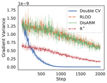
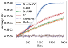
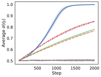
Figure 1: Variance reduction for a toy 200-dimensional maximization problem, following Tucker et al., (2017), with binary variables and fitting probabilities $\sigma(\eta_{i})$ (where $\sigma(\eta_{i})=1$ is optimal); see Section 5.1. Left: Gradient variances for four different estimators. Middle: Objective function that we want to maximize. Right: Average of the estimated $\sigma(\eta_{i})$s. In the latter two panels two additional estimators are shown. The proposed double control variate estimator (Double CV) is the most effective one.

We apply our double control variate approach to toy learning examples (see Fig. 1) and for training variational autoencoders with binary latent variables. We show that our estimator outperforms other methods including standard RLOO, DisARM (Dong et al.,, 2020; Yin et al.,, 2020) and its improved version ARMS (Dimitriev and Zhou,, 2021) when using $K=2$ or more samples. Although we focus on binary latent variables in our experiments, our estimator is equally applicable to categorical latent variables.

2 BACKRGOUND

Assume $f(x)$ is a differentiable objective function, where $x$ is a $D$-dimensional vector. We want to maximize the expectation $\mathbb{E}_{q_{\eta}(x)}\left[f(x)\right]$ with respect to the parameters $\eta$ of some distribution $q_{\eta}(x)$. Since $f(x)$ can have a complex non-linear form, the expectation is generally intractable. For instance, such problems arise in variational inference (Blei et al.,, 2017), where $f(x)$ is the instantaneous ELBO and $q_{\eta}(x)$ the variational distribution, and in reinforcement learning, where $f(x)$ is a reward function and $q_{\eta}(x)$ is the policy (Weaver and Tao,, 2001).

To apply gradient-based optimization over $\eta$ we need to compute the gradient

$$\nabla_{\eta}\mathbb{E}_{q_{\eta}(x)}\left[f(x)\right]=\mathbb{E}_{q_{\eta}(x)}\left[f(x)\nabla_{\eta}\log q_{\eta}(x)\right],$$ (1)

where for simplicity we assume $f(x)$ does not depend on $\eta$. Since this exact gradient is intractable, several techniques apply stochastic optimization (Robbins and Monro,, 1951) based on unbiased Monte Carlo gradients by sampling from $q_{\eta}(x)$. A very general stochastic gradient is the score function or REINFORCE estimator (Glynn,, 1990; Williams,, 1992; Carbonetto et al.,, 2009; Paisley et al.,, 2012; Ranganath et al.,, 2014; Mnih and Gregor,, 2014),

$$\frac{1}{K}\sum_{k=1}^{K}\left(f(x_{k})-b\right)\nabla_{\eta}\log q_{\eta}(x_{k}),\ \ x_{k}\sim q_{\eta}(x),$$ (2)

where $b$ is called a baseline and is often learned to reduce the variance. Given $K\geq 2$ samples, a powerful variant of this approach that avoids learning $b$ is the REINFORCE leave-one-out (RLOO) estimator (Salimans and Knowles,, 2014; Kool et al.,, 2019; Richter et al.,, 2020) that takes advantage of multiple evaluations of $f$:

$$\!\frac{1}{K}\!\sum_{k=1}^{K}\!\left(f(x_{k})-\frac{1}{K-1}\sum_{j\neq k}f(x_{j})\right)\nabla_{\eta}\log q_{\eta}(x_{k}),$$ (3)

where each leave-one-out average $\frac{1}{K-1}\sum_{j\neq k}f(x_{j})$ acts as a sample-specific control variate that excludes the current sample $x_{k}$, so that the whole estimator is unbiased. This estimator can also be re-written as an unbiased covariance estimator, i.e. $\text{RLOO}(\eta)=\frac{1}{K-1}\sum_{k=1}^{K}\left(f(x_{k})-\frac{1}{K}\sum_{j=1}^{K}f(x_{j})\right)\nabla_{\eta}\log q_{\eta}(x_{k})$, which could be more convenient in implementation (Kool et al.,, 2019; Richter et al.,, 2020).

RLOO was shown to have strong empirical performance, especially for discrete variable problems (Dong et al.,, 2020; Kool et al.,, 2019; Dong et al.,, 2021). It has the attractive property that the sample-specific control variates automatically adapt to the non-stationarity of $f(x)$. Specifically, the function $f(x):=f_{\theta}(x)$ can often contain additional model parameters $\theta$ updated at each optimization step (for $\theta$ is straightforward to obtain low variance gradients), as for instance in variational autoencoders (VAEs) (Kingma and Welling,, 2014; Rezende et al.,, 2014). Although $\theta$ is changing, the sample-specific control variate $\frac{1}{K-1}\sum_{j\neq k}f_{\theta}(x_{j})$ always remains an unbiased estimate of $\mathbb{E}_{q_{\eta}(x)}[f_{\theta}(x)]$.

However, RLOO is still limited in how much variance reduction it can achieve, as stated in the following proposition which is proved in the Appendix.

Proposition 1

Consider the estimator $\text{R}^{*}(\eta)=\frac{1}{K}\sum_{k=1}^{K}\left(f(x_{k})-\mathbb{E}f\right)\nabla_{\eta}\log q_{\eta}(x_{k})$, where $\mathbb{E}f=\mathbb{E}_{q_{\eta}(x)}[f(x)]$ is a constant baseline across all samples. Then, $Var(\text{RLOO})\geq Var(\text{R}^{*})$.

Thus, the performance of RLOO is bounded by $\text{R}^{*}$ which uses the mean $\mathbb{E}f$ (intractable in practice) as a constant baseline. However, an estimator with a constant baseline, even an ideal one as $\text{R}^{*}$, can often have substantial variance in practice. For instance, in the toy example shown by Fig. 1, where $\text{R}^{*}$ is tractable, we compare our proposed double control variates method with both RLOO and $\text{R}^{*}$, and show that our technique can outperform $\text{R}^{*}$ significantly. Our proposed estimator in Section 3 tries to further reduce the variance of RLOO and can be considered as using more general sample-specific baselines, as outlined in Section 2.1.

2.1 More General Sample-Specific Control Variates

Let’s denote by $x_{1:K}$ all $K$ samples in the estimator. We say a baseline $\gamma_{k}(x_{1:K})$ is sample-specific if it varies with the sample index $k$ in the Monte Carlo sum, i.e. $\gamma_{k}(x_{1:K})\neq\gamma_{j}(x_{1:K})$ for $k\neq j$. Note that each $\gamma_{k}(x_{1:K})$ can depend on all samples including also the “current” sample $x_{k}$. A general estimator with sample-specific control variates is written as

$$\frac{1}{K}\sum_{k=1}^{K}\left\{\left(f(x_{k})-\gamma_{k}(x_{1:K})\right)\nabla_{\eta}\log q_{\eta}(x_{k})\right\}$$

$$+\frac{1}{K}\sum_{k=1}^{K}\mathbb{E}_{q_{\eta}(x_{k})}[\gamma_{k}(x_{1:K})\nabla_{\eta}\log q_{\eta}(x_{k})].$$ (4)

The added sample-specific correction term $\mathbb{E}_{q_{\eta}(x_{k})}[\gamma_{k}(x_{1:K})\nabla_{\eta}\log q_{\eta}(x_{k})]$ must be analytically tractable and ensures that the gradient is unbiased. In some cases the correction term can be dropped, since it will have overall zero expectation, as stated next.

Proposition 2

Let $x_{1:k-1,k+1:K}$ denote all samples excluding $x_{k}$. If $\mathbb{E}_{q_{\eta}(x_{1:k-1,k+1:K})}[\gamma_{k}(x_{1:K})]=\text{const}$, then $\mathbb{E}_{q_{\eta}(x_{1:K})}[\gamma_{k}(x_{1:K})\nabla_{\eta}\log q_{\eta}(x_{k})]=0$.

See Appendix for the proof. A special case of this arises in REINFORCE LOO where the baseline $\gamma_{k}(x_{1:k-1,k+1:K})$ does not depend on the current sample $x_{k}$. However, more effective estimators can have a $\gamma_{k}$ depending on the current sample $x_{k}$ as well. For instance, such an estimator is the second variant (see equation (11)) of the double control variates approach presented next.

3 DOUBLE CONTROL VARIATES FOR REINFORCE LOO

In RLOO the sample-specific baseline $\frac{1}{K-1}\sum_{j\neq k}f(x_{j})$ is constant with respect to $x_{k}$. Also it is stochastic and as shown by Proposition 1 its variance is lower bounded by the estimator with $\mathbb{E}f$ as the baseline. Therefore, there is scope to further reduce the variance of this estimator, and the approach we follow is to consider additional control variates. We refer to these control variates as double since they act on top of the main RLOO baseline. We construct these new control variates along two directions:

1. We want to add a different type of control variate that depends on $x_{k}$ which may have a complementary effect to the main RLOO baseline.

2. Since the main baseline $\frac{1}{K-1}\sum_{j\neq k}f(x_{j})$ is stochastic and thus has variance, we can try to reduce the variance by adding a separate control variate for each stochastic random term $f(x_{j})$.

In the remaining of Section 3 we simplify notation by using $s(x):=\nabla_{\eta}\log q_{\eta}(x)$ to denote the score function. To accomplish both (a) and (b) simultaneously we start with the unbiased estimator

$$\frac{1}{K}\sum_{k=1}^{K}\left[f(x_{k})+\alpha b(x_{k})\right]s(x_{k})-\alpha\mathbb{E}_{q_{\eta}(x)}[b(x)s(x)],$$ (5)

where we introduced a control variate $b(x_{k})$, that depends on the current sample $x_{k}$ and has analytic global correction $\mathbb{E}_{q_{\eta}(x)}[b(x)s(x)]$. Then, to create a double control variate estimator we treat $f(x)+\alpha b(x)$ as the “new effective objective function” and apply the leave-one-out procedure to it. This leads to the following unbiased estimator

$$\frac{1}{K}\!\!\sum_{k=1}^{K}\!\!\left[f(x_{k})\!+\!\alpha{\color[rgb]{0,0,1}b(x_{k})}\!-\!\frac{1}{K\!\!-\!\!1}\sum_{j\neq k}\!(f(x_{j})\!+\!\alpha{\color[rgb]{1,0,0}b(x_{j})})\!\right]\!\!s(x_{k})$$

$$-\alpha\mathbb{E}_{q_{\eta}(x)}[b(x)s(x)].$$ (6)

The scalar $\alpha$ is a regression coefficient that can be further optimized to reduce the variance; see Section 3.3. In the above estimator we have highlighted with blue the first appearance $b(x_{k})$, that can be thought of as a baseline paired with the value $f(x_{k})$, and with red the second appearances $b(x_{j})$ paired with the remaining values $f(x_{j})$ of the main RLOO baseline. Intuitively, $b(x_{k})$ can be considered as targeting to reduce the variance of $f(x_{k})$ and $b(x_{j})$ the variance of $f(x_{j})$.

In Sections 3.1 and 3.2 we describe two ways to specify $b(x)$. For training latent variable models, such as VAEs, the second one will be the most practical since it adds no extra cost. The first method helps to introduce the idea and it is based on a mean field argument.

3.1 Mean Field Approach

The optimal choice of $b(x)$ is to become an exact surrogate of $f(x)$. This motivates to construct $b(x)$ by applying some tractable approximation to $f(x)$. While any surrogate of $f(x)$ with a tractable global correction could work, next we focus on the case when $f(x)$ is differentiable w.r.t. the input $x$. Specifically, we assume the target function $f$ is implemented as differentiable function of real-valued inputs, but is restricted on a discrete subset of its domain. Then, we construct $b(x)$ from a first order Taylor approximation around the mean $\mu=\mathbb{E}_{q_{\eta}(x)}[x]$, so that $f(x)\approx f(\mu)+\nabla f(\mu)^{\top}(x-\mu)=b(x)$. Furthermore, observe that any constant term in $b(x)$ can be ignored because it cancels out in (6). Thus, the constant $f(\mu)$ in the Taylor approximation can be dropped, yielding the double control variate

$$b(x)=\nabla f(\mu)^{\top}(x-\mu).$$ (7)

By substituting this in (6) we obtain the estimator

$$\frac{1}{K}\sum_{k=1}^{K}\bigg{[}f(x_{k})+\alpha\nabla f(\mu)^{\top}(x_{k}-\mu)$$

$$-\frac{1}{K\!-\!1}\sum_{j\neq k}\left(f(x_{j})+\alpha\nabla f(\mu)^{\top}(x_{j}-\mu)\right)\!\bigg{]}s(x_{k})$$

$$-\alpha\mathbb{E}_{q_{\eta}(x)}[s(x)(x-\mu)^{\top}]\nabla f(\mu),$$ (8)

where $\mathbb{E}_{q_{\eta}(x)}[s(x)(x-\mu)^{\top}]$ will typically be analytically tractable. For instance, for binary latent variables $x\in\{0,1\}^{d}$ and a factorised Bernoulli distribution

$$q_{\eta}(x)=\prod_{i=1}^{d}\mu_{i}^{x_{i}}(1-\mu_{i})^{1-x_{i}},\ \ \mu_{i}=\sigma(\eta_{i}),$$ (9)

$\mathbb{E}_{q_{\eta}(x)}[s(x)(x-\mu)^{\top}]=\text{diag}(\mu\circ(1-\mu))$ and the global correction term simplifies to $-\alpha\mu\circ(1-\mu)\circ\nabla f(\mu)$, where $\circ$ denotes element-wise vector product.

3.2 An Estimator without Extra Gradient Evaluations

The estimator in Eq. (8) requires a backpropagation operation to compute the gradient $\nabla f(\mu)$, which adds extra computational cost compared to standard RLOO. Next, we wish to develop an alternative estimator that avoids this extra cost for certain problems. For many applications, such as VAEs, the function $f(x)$ depends on model parameters $\theta$ (typically different than $\eta$) that we update at each optimization iteration by computing the gradients $\{\nabla_{\theta}f(x_{j})\}_{j=1}^{K}$. Then, from the same backpropagation operations it is easy to also return the gradients with respect to the latent vectors, i.e. to compute $\{\nabla_{x_{j}}f(x_{j})\}_{j=1}^{K}$. To simplify notation we will write $\nabla f(x):=\nabla_{x}f(x)$. We would like to utilize these latter gradients to define the double control variate $b(x)$.

Starting from (7) we first want to modify $b(x_{k})$ by replacing $\nabla f(\mu)$ with some new gradient computed from $\{\nabla f(x_{j})\}_{j=1}^{K}$. We cannot use the full average because this will lead to $(\frac{1}{K}\sum_{j=1}^{K}\nabla f(x_{j}))^{\top}(x_{k}-\mu)$ which has an intractable global correction due to the intractable term $\mathbb{E}_{q_{\eta}(x_{k})}[\nabla f(x_{k})^{\top}(x_{k}-\mu)\nabla_{\eta}\log q_{\eta}(x_{k})]$. However, we can use the leave-one-out gradient, i.e. by leaving out $\nabla f(x_{k})$, which gives

$$b_{k}(x_{1:K})=\left(\frac{1}{K-1}\sum_{j\neq k}\nabla f(x_{j})\right)^{\top}(x_{k}-\mu),$$ (10)

where we used the index $k$ in $b_{k}$ to emphasize that this now becomes a sample-specific control variate that varies with sample index; see Section 2.1. This has a tractable correction term $\mathbb{E}_{q_{\eta}(x_{k})}[b_{k}(x_{1:K})s(x_{k})]$ and also satisfies $\mathbb{E}_{q_{\eta}(x_{k})}[b_{k}(x_{1:K}]=0$. Having specified the double control variate we express the unbiased estimator as stated below.

Proposition 3

For $b_{k}(x_{1:K})$ from (10) we obtain the following unbiased gradient estimator

$$\frac{1}{K}\!\!\sum_{k=1}^{K}\!\!\bigg{[}\!f(x_{k})\!+\!\alpha b_{k}(x_{1:K})\!-\!\frac{1}{K\!\!-\!\!1}\!\sum_{j\neq k}\!\left(f(x_{j})\!+\!\alpha b_{j}(x_{1:K})\right)\!\!\bigg{]}$$

$$\!\times\!s(x_{k})\!-\!\alpha\mathbb{E}_{q_{\eta}(x)}[s(x)(x\!-\!\mu)^{\top}\!]\!\left(\!\frac{1}{K}\!\sum_{k=1}^{K}\!\nabla f(x_{k})\!\right).$$ (11)

The proof of unbiasedness is given in the Appendix. Notably, the above estimator follows the general structure from Eq. (4) for a certain choice of the sample-specific control variate.

3.3 Further Details and Algorithmic Summary

To apply the estimator in (11) we need to specify the regression coefficient $\alpha$ by minimizing the variance. If $g(\eta;\alpha)$ denotes the stochastic gradient and $\bar{g}=\mathbb{E}[g(\eta;\alpha)]$ the exact gradient where the latter does not depend on $\alpha$, the total variance is $\text{Tr}[\mathbb{E}(g(\eta;\alpha)-\bar{g})(g(\eta;\alpha)-\bar{g})^{\top}]=\mathbb{E}[||g(\eta;\alpha)||^{2}]+const$. Thus, in practice at each optimization iteration we can perform a gradient step towards minimizing the empirical variance $||g(\eta;\alpha)||^{2}$. There also exists an analytic formula (but requiring intractable expectations) for the optimal value of $\alpha$ that can inspire different types of learning rules; see Appendix for further details. The whole algorithm that also deals with a non-stationary $f_{\theta}(x)$, i.e., that includes $\theta$ updates at each iteration, is outlined in Algorithm 1. For the special case where $K=2$ the estimator (11) simplifies as

$$\Delta(x_{1},x_{2},\alpha)\frac{\nabla_{\eta}\log q_{\eta}(x_{1})\!-\!\nabla_{\eta}\log q_{\eta}(x_{2})}{2}$$

$$-\alpha\mathbb{E}_{q_{\eta}(x)}[s(x)(x-\mu)^{\top}]\frac{\nabla f(x_{1})+\nabla f(x_{2})}{2},$$ (12)

where $\Delta(x_{1},x_{2},\alpha)=f(x_{1})-f(x_{2})+\alpha[\nabla f(x_{2})^{\top}(x_{1}-\mu)-\nabla f(x_{1})^{\top}(x_{2}-\mu)]$. In the experiments we compare this estimator with the DisARM method (Dong et al.,, 2020; Yin et al.,, 2020) that uses $K=2$ antithetic samples, and also with RLOO with $K=2$ samples.

Algorithm 1 Optimization with double control variate gradients

  input: loss $f_{\theta}(x)$, distribution $q_{\eta}(x)$.

  Initialise $\theta$, $\eta$, $\alpha=0$.

  for $t=1,2,3,\ldots,$ do

1:  Draw $K$ samples $x_{1:K}$, $x_{k}\sim q_{\eta}(x)$.

2:  Compute $\mu=\mathbb{E}_{q_{\eta}(x)}[x]$.

3:  $[f(x_{k}),\!\!\nabla_{\theta}f(x_{k}),\!\!\nabla_{x_{k}}f(x_{k})]_{k=1}^{K}\leftarrow\!\text{grad}(f_{\theta},q_{\eta},x_{1:k}\!)$.

4:  Compute double control variates $b_{k}(x_{1:K})$ from Eq. (10).

5:  Compute double control variates gradient $g(\eta;\alpha)$ from Eq. (11).

6:  Adapt $\eta$: $\eta\leftarrow\eta-\rho_{t}\times g(\eta;\alpha)$.

7:  Adapt $\theta$: $\theta\leftarrow\theta-\hat{\rho}_{t}\times\frac{1}{K}\sum_{k=1}^{K}\nabla_{\theta}f_{\theta}(x_{k})$.

8:  Adapt regression scalar $\alpha$ by applying a gradient step to minimize $||g(\eta;\alpha)||^{2}$.

  end for

4 RELATED WORK

Table 1: Training nonlinear binary latent VAEs with $K=2$ (except RELAX which needs 3 evaluations of $f$) on MNIST, Fashion-MNIST, and Omniglot. We report the average training ELBO over 5 independent runs.

	Bernoulli Likelihoods			Gaussian Likelihoods
	MNIST	Fashion-MNIST	Omniglot	MNIST	Fashion-MNIST	Omniglot
RLOO	$-103.11\pm 0.16$	$-241.53\pm 0.24$	$-116.83\pm 0.05$	$668.07\pm 0.40$	$179.52\pm 0.23$	$443.51\pm 0.93$
Double CV	$\bf-102.45\pm 0.13$	$\bf-240.96\pm 0.17$	$\bf-116.22\pm 0.08$	$\bf 676.87\pm 1.18$	$\bf 186.35\pm 0.64$	$\bf 446.95\pm 0.63$
DisARM	$-102.56\pm 0.09$	$-241.02\pm 0.20$	$-116.36\pm 0.05$	$668.03\pm 0.61$	$182.65\pm 0.47$	$446.22\pm 1.38$
RELAX (3 evals)	$\bf-101.86\pm 0.11$	$\bf-240.63\pm 0.16$	$\bf-115.79\pm 0.06$	$\bf 688.58\pm 0.52$	$\bf 196.38\pm 0.66$	$\bf 462.30\pm 0.91$

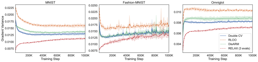
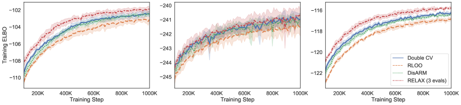
Figure 2: Training nonlinear binary latent VAEs with Bernoulli likelihoods with $K=2$ (except RELAX which needs 3 evaluations of $f$) on dynamically binarized MNIST, Fashion-MNIST, and Omniglot. Top: Variance of gradient estimates. Bottom: Average ELBO on training examples.

Our proposed gradient estimators follow the general form of unbiased REINFORCE estimators (Williams,, 1992; Glynn,, 1990; Carbonetto et al.,, 2009; Paisley et al.,, 2012; Ranganath et al.,, 2014; Mnih and Gregor,, 2014), which unlike reparametrization or pathwise gradients (Kingma and Welling,, 2014; Rezende et al.,, 2014; Titsias and Lázaro-Gredilla,, 2014), are applicable also to discrete latent variables. The double control variates we develop build on top of the RLOO estimator (Kool et al.,, 2019; Salimans and Knowles,, 2014; Richter et al.,, 2020); see also the VIMCO method of Mnih and Rezende, (2016) who also used a leave-one-out procedure. RLOO was shown to be a competitive estimator for challenging problems such as training VAEs with binary or categorical latent variables (Dong et al.,, 2020; Richter et al.,, 2020; Dong et al.,, 2021). As shown by our experiments, our enhancement of RLOO with double control variates leads to further variance reduction, and without increasing the computational cost when training VAEs.

In our current framework, the double control variates are constructed by using the gradients of the objective function $f_{\theta}(x)$. These gradients are also used by other unbiased gradient techniques based on control variates, such as the MuProp estimator (Gu et al.,, 2016), REBAR (Tucker et al.,, 2017) and RELAX (Grathwohl et al.,, 2018). Our method differs significantly since our control variates act on top of the sample-specific RLOO baseline $\frac{1}{K-1}\sum_{j\neq k}f_{\theta}(x_{j})$, i.e., they try to have complementary effect to this existing control variate. This means that our estimators preserve RLOO’s property of capturing the non-stationarity of $f_{\theta}(x)$, since the leave-one-out baseline always tracks the expected value $\mathbb{E}[f_{\theta}(x)]$ as $\theta$ evolves. In contrast, previous gradient-based estimators use stand-alone global control variates. For instance, the baseline in MuProp (Gu et al.,, 2016) is constructed using only $f_{\theta}(\mu)$ and $x_{k}$, which can be a poor tracker of the expected value $\mathbb{E}[f_{\theta}(x)]$. Unlike MuProp, REBAR (Tucker et al.,, 2017) is much more effective, however it is more expensive than our method — it requires differentiating $f_{\theta}$ three times, while our method can work with just two, and it is less generally applicable since they assume a continuous reparameterization for $q$. RELAX (Grathwohl et al.,, 2018) suffers from the same problem as its strong performance relies on the REBAR control variate (Richter et al.,, 2020).

Other recent REINFORCE type of estimators for discrete latent variables are based on coupled sampling (Owen,, 2013), such as antithetic sampling (Yin and Zhou,, 2019; Dong et al.,, 2020; Yin et al.,, 2020; Dimitriev and Zhou,, 2021). For instance, the recent DisARM estimator independently proposed by Dong et al., (2020) and Yin et al., (2020) was shown to give state-of-the-art results for binary latent-variable models with $K=2$ antithetic samples.

5 EXPERIMENTS

Code for reproducing all experiments is available at https://github.com/thjashin/double-cv.

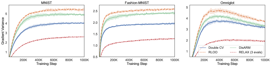
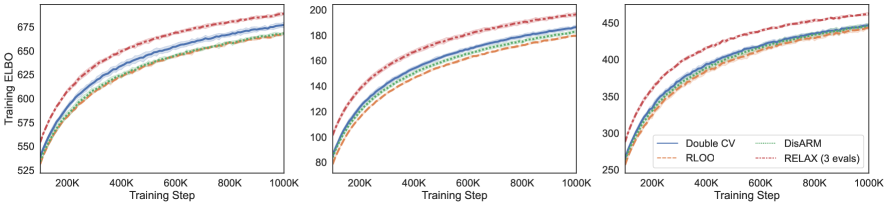
Figure 3: Training nonlinear binary latent VAEs with Gaussian likelihoods with $K=2$ (except RELAX which needs 3 evaluations of $f$) on non-binarized MNIST, Fashion-MNIST, and Omniglot. Top: Variance of gradient estimates. Bottom: Average ELBO on training examples.

5.1 Toy Learning Problem

We consider a generalization of the artificial problem considered by Tucker et al., (2017). The goal is to maximize $\mathcal{E}(\eta)=\mathbb{E}_{q_{\eta}(x)}[D^{-1}\sum_{i=1}^{D}(x_{i}-p_{0})^{2}],$ where $q_{\eta}(x)=\prod_{i=1}^{D}\sigma(\eta_{i})^{x_{i}}(1-\sigma(\eta_{i}))^{1-x_{i}}$, $p_{0}=0.499$ and the optimal solution is $\sigma(\eta_{i})=1$ for all $i=1,\ldots,D$. While Tucker et al., (2017) considered $D=1$, here we additionally consider a more difficult high-dimensional case with $D=200$. We compare five methods: RLOO, DisARM, MuProp, Reinforce (with no baselines) and our proposed double control variates estimator (Double CV) from Eq. (11). We use $K=2$ samples for all methods (note that Double CV in this case simplifies as in (12)). Also we include in the comparison $\text{R}^{*}$ which is tractable in this toy example. Fig. 1 compares the methods in terms of variance, the objective function and the average value of the $D$ probabilities $\sigma(\eta_{i})$. Fig. 6 in the Appendix shows further comparison for the $D=1$ case, as in Tucker et al., (2017). We observe that Double CV gradients have smaller variance which results in much faster optimization convergence.

5.2 Variational Autoencoders with Binary Latent Variables

Experimental setup

We consider training variational autoencoders (Kingma and Welling,, 2014; Rezende et al.,, 2014) with binary latent variables. We conduct separate experiments for binary output data $y\in\{0,1\}^{d}$ and continuous data $y\in\mathbb{R}^{d}$. For binary data we use the standard Bernoulli likelihood. For continuous data we centered data between $[-1,1]$ and consider a Gaussian likelihood of the form $p_{\theta}(y|x)=\mathcal{N}(y|m_{\theta}(x),\Sigma)$, where $m_{\theta}(x)$ is a decoder mean function that depends on the latent variable $x$ and $\Sigma$ is a learnable diagonal covariance matrix. We consider the datasets MNIST, Fashion-MNIST and Omniglot. For all three datasets we use both the dynamically binarized versions and their original continuous versions.

We consider the nonlinear VAE models used in Yin and Zhou, (2019); Dong et al., (2020); results for linear VAEs are included in the Appendix. The VAE model uses fully connected neural networks with two hidden layers of $200$ LeakyReLU activation units with the coefficient $0.3$. All models are trained using Adam (Kingma and Ba,, 2014) with learning rate $10^{-3}$ for the binarized data, while for the continuous data we used smaller learning rate $10^{-4}$. In all experiments the regression coefficient $\alpha$ of the double control variates was also trained (see Section 3.3) with Adam and with learning rate $10^{-3}$. For all experiments we use a uniform factorized Bernoulli prior over the $D=200$ dimensional latent variable $x$. The model was trained by maximizing the ELBO using an amortised factorised variational Bernoulli distribution.

Table 2: Training a nonlinear binary latent VAE with $K=4$ (except RELAX which needs 3 evaluations of $f$) on MNIST, Fashion-MNIST, and Omniglot. We report the average training ELBO over 5 independent runs.

	Bernoulli Likelihoods			Gaussian Likelihoods
	MNIST	Fashion-MNIST	Omniglot	MNIST	Fashion-MNIST	Omniglot
RLOO	$-100.50\pm 0.22$	$-239.03\pm 0.15$	$-114.75\pm 0.07$	$687.83\pm 0.50$	$195.27\pm 0.24$	$460.23\pm 1.42$
Double CV	$\bf-99.89\pm 0.12$	$-238.98\pm 0.18$	$\bf-114.56\pm 0.06$	$\bf 691.51\pm 0.75$	$\bf 199.01\pm 0.60$	$463.03\pm 0.94$
DisARM	$-100.67\pm 0.07$	$-239.20\pm 0.15$	$-115.05\pm 0.07$	$683.28\pm 0.89$	$192.96\pm 0.29$	$458.38\pm 0.88$
ARMS	$-100.07\pm 0.08$	$\bf-238.50\pm 0.13$	$-114.57\pm 0.06$	$687.26\pm 1.21$	$197.25\pm 0.48$	$\bf 463.30\pm 0.86$
RELAX (3 evals)	$-101.86\pm 0.11$	$-240.63\pm 0.16$	$-115.79\pm 0.06$	$688.58\pm 0.52$	$196.38\pm 0.66$	$462.30\pm 0.91$

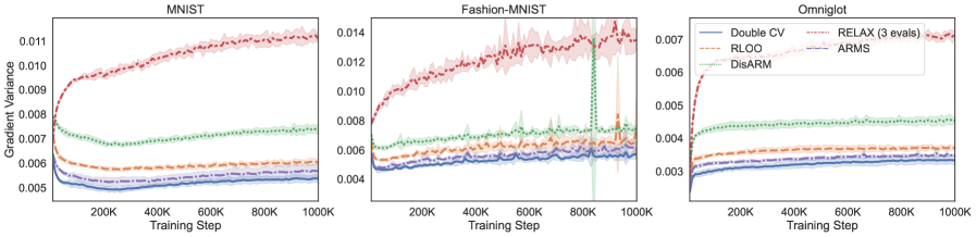
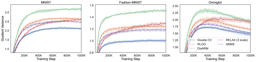
Figure 4: Variance of gradient estimates in training nonlinear binary latent variational autoencoders with $K=4$ (except RELAX which needs 3 evaluations of $f$) on MNIST, Fashion-MNIST, and Omniglot. Top: Using Bernoulli likelihoods and dynamically binarized datasets. Bottom: Using Gaussian likelihoods and non-binarized datasets.

We compared the following estimators: RLOO, DisARM and the proposed Double CV method where all three estimators use $K$ samples. We experimented with $K=2$ and $K=4$. For $K=4$ we also compare to the state-of-the-art ARMS estimator recently proposed by Dimitriev and Zhou, (2021). Besides, we include in the comparison the RELAX estimator that combines concrete relaxation (Tucker et al.,, 2017) with a learned control variate (Grathwohl et al.,, 2018). We point out that RLOO, DisARM, Double CV, and ARMS (when $K=4$) have roughly the same running time on a P100 GPU while RELAX is computationally more expensive and is roughly twice slower than the other four estimators with $K=4$ (see Table 3 in the Appendix). Also note that RELAX is less generally applicable since it assumes the existence of a continuous relaxation for $x$.

Results

Table 1 shows the training ELBO for binarized and continuous datasets when training the VAE by different estimators with $K=2$. We can observe that Double CV consistently outperforms RLOO in all experiments, while having approximately the same running time. Double CV also outperforms DisARM in all cases for both Bernoulli and Gaussian likelihoods. Furthermore, Fig. 2 plots the gradient variance and the training ELBO for the binarized datasets as a function of the training steps. Similarly, Fig. 3 shows the corresponding results for the non-binarized (continuous) datasets where a Gaussian likelihood is used. We observe that the Double CV estimator can have lower variance than RLOO and DisARM. Also, while RELAX performs better than the other methods it is less generally applicable and more expensive.

For $K=4$, the final training ELBO values are reported in Table 2 and the variances of the different estimators are plotted in Fig. 4. We can observe that Double CV consistently has lower variance than other estimators and it outperforms ARMS in terms of training ELBO in most cases. It also significantly outperforms RELAX. Note that, even with $K=4$, Double CV is still nearly twice faster than RELAX.

6 CONCLUSION

We presented a new variance reduction technique called double control variates for gradient estimation of discrete latent variable models. We achieved substantial variance reduction by constructing control variates on top of existing leave-one-out baselines in REINFORCE estimators. The proposed estimator is unbiased and adds no extra computational cost to the standard backpropagation cost needed for obtaining gradients over model parameters.

Finally, the use of double control variates can be orthogonal to other techniques for variance reduction such as coupled sampling (Yin and Zhou,, 2019; Dong et al.,, 2020, 2021; Dimitriev and Zhou,, 2021) and concrete relaxations (Tucker et al.,, 2017; Grathwohl et al.,, 2018). This could lead to various combinations of our approach with these techniques. For instance, if we start from our initial estimator in (5) where we simply replace the initial objective function $f(x)$ with the new effective objective $f(x)+\alpha b(x)$, a combination with coupled sampling is possible, e.g. certainly this holds for the mean field choice $b(x)=\nabla f(\mu)^{\top}(x-\mu)$. Also if we relax the restriction of the global correction $\mathbb{E}_{q_{\eta}(x)}[b(x)\nabla_{\eta}\log q_{\eta}(x)]$ to be analytic but instead allow to be reparametrizable, then our method could be combined with the concrete relaxation methods. The investigation of such combinations is an interesting topic for future research.

Appendix A Proofs

A.1 Proof of Proposition 1

The RLOO estimator can be written as

$$\underbrace{\frac{1}{K}\sum_{k=1}^{K}\left(f(x_{k})-\mathbb{E}f\right)\nabla_{\eta}\log q_{\eta}(x_{k})}_{\text{R}^{*}}+\underbrace{\frac{1}{K}\sum_{k=1}^{K}\left(\mathbb{E}f-\frac{1}{K-1}\sum_{j\neq k}f(x_{j})\right)\nabla_{\eta}\log q_{\eta}(x_{k})}_{E}$$ (13)

where $\text{R}^{*}$ is the REINFORCE estimator with baseline $\mathbb{E}f$ and $E$ is a residual term of zero mean. To prove the Proposition we will use $Var(\text{RLOO})=Var(\text{R}^{*}+E)=Var(\text{R}^{*})+Var(E)+2Cov(\text{R}^{*},E)$. Then, it suffices to show that $Cov(\text{R}^{*},E)=0$. We have

$$Cov(\text{R}^{*},E)=\frac{1}{K^{2}}\sum_{k=1}^{K}\sum_{k^{\prime}=1}^{K}\mathbb{E}\left[(f(x_{k})-\mathbb{E}f)(\mathbb{E}f-f_{-k^{\prime}})\nabla_{\eta}\log q_{\eta}(x_{k})\nabla_{\eta}\log q_{\eta}(x_{k^{\prime}})^{\top}\right]$$

where we used $f_{-k^{\prime}}=\frac{1}{K-1}\sum_{j\neq k^{\prime}}f(x_{j})$ for short. For all terms in the double sum such that $k=k^{\prime}$ the expectation

$$\mathbb{E}\left[(f(x_{k})-\mathbb{E}f)(\mathbb{E}f-f_{-k})\nabla_{\eta}\log q_{\eta}(x_{k})\nabla_{\eta}\log q_{\eta}(x_{k})^{\top}\right]=0$$

because the zero-mean random variable $\mathbb{E}f-f_{-k}$ is independent from the remaining product (since it does not contain the sample $x_{k}$). For all cross terms $k\neq k^{\prime}$ the whole product $(f(x_{k})-\mathbb{E}f)(\mathbb{E}f-f_{-k^{\prime}})\nabla_{\eta}\log q_{\eta}(x_{k})$ does not contain the sample $x_{k^{\prime}}$. Therefore this product is independent from $\nabla_{\eta}\log q_{\eta}(x_{k^{\prime}})$ and thus each cross term is zero because of the score function property $\mathbb{E}[\nabla_{\eta}\log q_{\eta}(x_{k^{\prime}})]=0$. This shows that $Cov(\text{R}^{*},E)=0$ which completes the proof.

A.2 Proof of Proposition 2

It holds

$$\mathbb{E}_{q_{\eta}(x_{1:K})}[\gamma_{k}(x_{1:K})\nabla_{\eta}\log q_{\eta}(x_{k})]$$

$$=\mathbb{E}_{q_{\eta}(x_{k})}\bigg{[}\mathbb{E}_{q_{\eta}(x_{1:k-1},x_{k+1:K})}[\gamma_{k}(x_{1:K})]\nabla_{\eta}\log q_{\eta}(x_{k})\bigg{]}$$

$$=\mathbb{E}_{q_{\eta}(x_{k})}\bigg{[}\text{const}\nabla_{\eta}\log q_{\eta}(x_{k})\bigg{]}=0.$$ (14)

where the last line is just a consequence of the score function property since const does not depend on $x_{k}$.

A.3 Proof of Proposition 3

The estimator can be written as

$$\frac{1}{K}\sum_{k=1}^{K}\left[f(x_{k})-\frac{1}{K-1}\sum_{j\neq k}f(x_{j})\right]\nabla_{\eta}\log q_{\eta}(x_{k})$$

$$+\alpha\frac{1}{K}\sum_{k=1}^{K}\left({\color[rgb]{0,0,1}b_{k}(x_{1:K})}-\frac{1}{K-1}\sum_{j\neq k}{\color[rgb]{1,0,0}b_{j}(x_{1:K})}\right)\nabla_{\eta}\log q_{\eta}(x_{k})$$

$$-\alpha\mathbb{E}_{q(x)}[\nabla_{\eta}\log q_{\eta}(x)\times(x-\mu)^{\top}]\left(\frac{1}{K}\sum_{k=1}^{K}\nabla f(x_{k})\right),$$ (15)

where $b_{k}(x_{1:K})=\left(\frac{1}{K-1}\sum_{j\neq k}\nabla f(x_{j})\right)^{\top}(x_{k}-\mu)$ and $b_{j}(x_{1:K})=\left(\frac{1}{K-1}\sum_{m\neq j}\nabla f(x_{m})\right)^{\top}(x_{j}-\mu)$. It suffices to show that the expectation of the second line is minus the correction term at the third line. The expectation of each term $b_{j}(x_{1:K})\nabla_{\eta}\log q_{\eta}(x_{k})$ for $j\neq k$ is zero because the zero-mean term $x_{j}-\mu$ is always independent from the rest of the terms in the product. Then, we need to examine only the expectation of

$$\frac{1}{K}\sum_{k=1}^{K}{\color[rgb]{0,0,1}b_{k}(x_{1:K})}\nabla_{\eta}\log q_{\eta}(x_{k})=\frac{1}{K(K-1)}\sum_{k=1}^{K}\nabla_{\eta}\log q_{\eta}(x_{k})(x_{k}-\mu)^{\top}\sum_{j\neq k}\nabla f(x_{j}).$$

Then observe that the expectation of $\nabla_{\eta}\log q_{\eta}(x_{k})\times(x_{k}-\mu)^{\top}$ is the same for every sample $x_{k}$, so the above reduces to

$$\mathbb{E}_{q_{\eta}(x)}[\nabla_{\eta}\log q_{\eta}(x)\times(x-\mu)^{\top}]\frac{1}{K(K-1)}\sum_{k=1}^{K}\sum_{j\neq k}\nabla f(x_{j})$$

from which the result follows since $\sum_{k=1}^{K}\sum_{j\neq k}\nabla f(x_{j})=(K-1)\sum_{k=1}^{K}\nabla f(x_{k})$.

A.4 The Optimal Value of $\alpha$ for $K=2$

The gradient for $K=2$ can be written as

$$\frac{1}{2}[f(x_{1})-f(x_{2})](\nabla_{\eta}\log q_{\eta}(x_{1})-\nabla_{\eta}\log q_{\eta}(x_{2}))$$

$$-\frac{1}{2}\alpha\left(M(\nabla f(x_{1})+\nabla f(x_{2}))-[\nabla f(x_{2})^{\top}(x_{1}-\mu)-\nabla f(x_{1})^{\top}(x_{2}-\mu)](\nabla_{\eta}\log q_{\eta}(x_{1})-\nabla_{\eta}\log q_{\eta}(x_{2}))\right)$$ (16)

where $M=\mathbb{E}_{q_{\eta}(x)}[\nabla_{\eta}\log q_{\eta}(x)\times(x-\mu)^{\top}]$. If we denote

$$g(x_{1},x_{2})=[f(x_{1})-f(x_{2})](\nabla_{\eta}\log q_{\eta}(x_{1})-\nabla_{\eta}\log q_{\eta}(x_{2}))$$

and

$$h(x_{1},x_{2})=M(\nabla f(x_{1})+\nabla f(x_{2}))-[\nabla f(x_{2})^{\top}(x_{1}-\mu)-\nabla f(x_{1})^{\top}(x_{2}-\mu)](\nabla_{\eta}\log q_{\eta}(x_{1})-\nabla_{\eta}\log q_{\eta}(x_{2}))$$

the gradient can be written as

$$\frac{1}{2}\left(g(x_{1},x_{2})-\alpha h(x_{1},x_{2})\right).$$

Then the optimal $\alpha$ that minimizes the variance is given by

$$\alpha=\frac{\mathbb{E}[g(x_{1},x_{2})^{\top}h(x_{1},x_{2})]}{\mathbb{E}[h(x_{1},x_{2})^{\top}h(x_{1},x_{2})]}$$

Similarly we can construct the optimal value of $\alpha$ for any $K>2$.

A.5 The “half” Double Control Variate Estimators

One question is whether we need both $b(x_{k})$ and $b(x_{j})$ or we could keep one of them, i.e. to use an “$b(x_{k})$ only” or “$b(x_{j})$ only” estimator. It is straightforward to express these latter unbiased estimators, as follows. The “$b(x_{k})$ only” estimator is given by

$$\frac{1}{K}\!\!\sum_{k=1}^{K}\!\!\left[f(x_{k})+\alpha{\color[rgb]{0,0,1}b(x_{k})}\!-\!\frac{1}{K\!-\!1}\sum_{j\neq k}\!f(x_{j})\right]\!\nabla_{\eta}\log q_{\eta}(x_{k})-\alpha\mathbb{E}_{q_{\eta}(x)}[b(x)\nabla_{\eta}\!\log q_{\eta}(x)].$$ (17)

and the “$b(x_{j})$ only” by

$$\frac{1}{K}\!\!\sum_{k=1}^{K}\!\!\left[f(x_{k})\!-\!\frac{1}{K\!-\!1}\sum_{j\neq k}\!(f(x_{j})+\alpha{\color[rgb]{1,0,0}b(x_{j})})\right]\!\nabla_{\eta}\log q_{\eta}(x_{k}).$$ (18)

It is easy to show that both estimators are unbiased. However, in practice these estimators can be much less effective in terms of variance reduction than their Double CV combination. In Fig. 5 we apply these two estimators to the toy learning problem with $D=10$. Both estimators are significantly outperformed by the full Double CV estimator. Notably, the “$b(x_{k})$ only” estimator could outperform $\text{R}^{*}$ since it uses a baseline that depends on the current sample $x_{k}$, while “$b(x_{j})$ only” reduces the variance of the RLOO control variate but remains bounded by $\text{R}^{*}$.

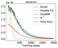
Figure 5: Left: Variance of the “only $b(x_{k})$” estimator where only the half part of the double control variate is used. Right: The corresponding plot for the “only $b(x_{j})$” estimator where the other half part of the double control variate is used. The full double control variate estimator (Double CV), RLOO, DisARM and $\text{R}^{*}$ are included for comparison. The experiment corresponds to the toy problem with $D=10$ and $b(x)$ was chosen according to Eq. (10), i.e. the full Double CV estimator is from (11).

Appendix B Additional Results

B.1 Toy Experiment with $D=1$

For completeness, we include the results of a simpler version of the toy experiment described in Section 5.1, where we set $D=1$. This is the setting used in several previous works (Tucker et al.,, 2017; Grathwohl et al.,, 2018; Yin and Zhou,, 2019; Dong et al.,, 2020). The variances of the gradient estimators and the training curves of $\sigma(\eta)$ are plotted in Fig. 6. Fig. 7 shows the evolution of the estimated regression coefficient $\alpha$.

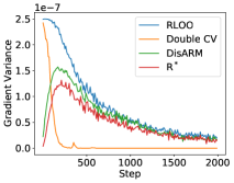
Figure 6: Left: Variance of the gradient estimators for the toy problem with $D=1$. Right: The estimated value $\sigma(\eta)$ across iterations (optimal value is $1$).

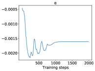
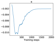
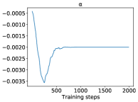
$D=1$	$D=10$	$D=200$

Figure 7: The evolution of the estimated regression coefficient $\alpha$ during optimization for the toy learning problem.

B.2 Training Binary Latent VAEs

B.2.1 Time comparison

In Fig. 3 we report the per-step running time of RLOO, Double CV, DisARM, ARMS estimators when $K=4$ and compare to RELAX. RELAX is almost twice slower.

	RLOO	Double CV	DisARM	ARMS	RELAX
Time (sec/step)	0.0035	0.0036	0.0031	0.0037	0.0080

Table 3: Time per step when training a Bernoulli VAE with $K=4$ (except RELAX which needs 3 evaluations of $f$) on dynamically binarized Fashion-MNIST.

	RLOO	Double CV	DisARM	RELAX (3 evals)
MNIST:
Linear	$-113.06\pm 0.05$	$-112.82\pm 0.07$	$\bf-112.72\pm 0.07$	$\bf-112.18\pm 0.07$
Nonlinear	$-103.11\pm 0.16$	$\bf-102.45\pm 0.13$	$-102.56\pm 0.09$	$\bf-101.86\pm 0.11$
Fashion-MNIST:
Linear	$-257.38\pm 0.17$	$\bf-256.21\pm 0.17$	$-257.01\pm 0.06$	$\bf-255.16\pm 0.17$
Nonlinear	$-241.53\pm 0.24$	$\bf-240.96\pm 0.17$	$-241.02\pm 0.20$	$\bf-240.63\pm 0.16$
Omniglot:
Linear	$-119.63\pm 0.05$	$-119.52\pm 0.02$	$\bf-119.42\pm 0.03$	$\bf-119.16\pm 0.02$
Nonlinear	$-116.83\pm 0.05$	$\bf-116.22\pm 0.08$	$-116.36\pm 0.05$	$-\bf 115.79\pm 0.06$

Table 4: Training binary latent VAEs with $K=2$ (except RELAX which needs 3 evaluations of $f$) on dynamically binarized MNIST, Fashion-MNIST, and Omniglot. We report the average ELBO on the training set over 5 independent runs.

	RLOO	Double CV	DisARM	RELAX (3 evals)
MNIST
Linear	$503.01\pm 0.22$	$504.33\pm 0.98$	$\bf 504.43\pm 0.93$	$\bf 513.38\pm 0.52$
Nonlinear	$668.07\pm 0.40$	$\bf 676.87\pm 1.18$	$668.03\pm 0.61$	$\bf 688.58\pm 0.52$
Fashion-MNIST
Linear	$29.75\pm 0.40$	$31.08\pm 0.24$	$\bf 31.71\pm 0.20$	$\bf 37.54\pm 0.30$
Nonlinear	$179.52\pm 0.23$	$\bf 186.35\pm 0.64$	$182.65\pm 0.47$	$\bf 196.38\pm 0.66$
Omniglot
Linear	$245.73\pm 0.33$	$245.97\pm 1.02$	$\bf 247.70\pm 0.85$	$\bf 255.69\pm 0.70$
Nonlinear	$443.51\pm 0.93$	$\bf 446.95\pm 0.63$	$446.22\pm 1.38$	$\bf 462.30\pm 0.91$

Table 5: Training binary latent VAEs with Gaussian likelihoods using $K=2$ (except RELAX which needs 3 evaluations of $f$) on non-binarized MNIST, Fashion-MNIST, and Omniglot. We report the average ELBO on the training set over 5 independent runs.

B.2.2 Full results of training ELBOs

Here we include the full results of final training ELBOs from the experiment in Section 5.2. Table 4 and Table 5 extend Table 1 to include the linear VAE results trained under the same setting. Table 6 and Table 7 extend Table 2 to include the linear VAE results trained under the same setting. The linear VAE has $200$ dimensional latent variable $x$ and use a single fully-connected layer to produce the logits (for Bernoulli likelihoods) or the mean (for Gaussian likelihoods) of the distribution of $y$.

	RLOO	Double CV	DisARM	ARMS
MNIST:
Linear	$-111.89\pm 0.09$	$\bf-111.79\pm 0.09$	$-112.01\pm 0.06$	$-111.87\pm 0.02$
Nonlinear	$-100.50\pm 0.22$	$\bf-99.89\pm 0.12$	$-100.67\pm 0.07$	$-100.07\pm 0.08$
Fashion-MNIST:
Linear	$-254.59\pm 0.16$	$\bf-254.52\pm 0.23$	$-255.01\pm 0.10$	$-254.67\pm 0.20$
Nonlinear	$-239.03\pm 0.15$	$-238.98\pm 0.18$	$-239.20\pm 0.15$	$\bf-238.50\pm 0.13$
Omniglot:
Linear	$-118.89\pm 0.02$	$-118.95\pm 0.02$	$-118.97\pm 0.01$	$\bf-118.87\pm 0.02$
Nonlinear	$-114.75\pm 0.07$	$\bf-114.56\pm 0.06$	$-115.05\pm 0.07$	$-114.57\pm 0.06$

Table 6: Training binary latent VAEs with $K=4$ on dynamically binarized MNIST, Fashion MNIST, and Omniglot. We report the average ELBO on the training set over 5 independent runs.

	RLOO	Double CV	DisARM	ARMS
MNIST:
Linear	$\bf 516.65\pm 0.54$	$515.79\pm 0.71$	$512.47\pm 0.72$	$514.55\pm 0.71$
Nonlinear	$687.83\pm 0.50$	$\bf 691.51\pm 0.75$	$683.28\pm 0.89$	$687.26\pm 1.21$
Fashion-MNIST:
Linear	$36.70\pm 0.41$	$36.61\pm 0.34$	$34.90\pm 0.52$	$\bf 37.56\pm 0.43$
Nonlinear	$195.27\pm 0.24$	$\bf 199.01\pm 0.60$	$192.96\pm 0.29$	$197.25\pm 0.48$
Omniglot:
Linear	$257.43\pm 0.16$	$257.88\pm 0.69$	$254.99\pm 0.69$	$\bf 258.22\pm 0.18$
Nonlinear	$460.23\pm 1.42$	$463.03\pm 0.94$	$458.38\pm 0.88$	$\bf 463.30\pm 0.86$

Table 7: Training binary latent VAEs with Gaussian likelihoods using $K=4$ on non-binarized MNIST, Fashion-MNIST, and Omniglot. We report the average ELBO on the training set over 5 independent runs.

B.2.3 Additional figures for nonlinear VAEs

In Fig. 8 we plot the average training ELBOs as a function of training steps from the $K=4$ experiment in Section 5.2.

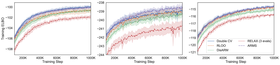
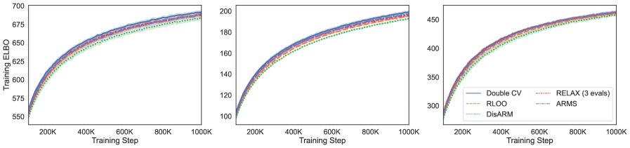
Figure 8: Average training ELBOs for nonlinear binary latent VAEs trained by different estimators with $K=4$ (except RELAX which needs 3 evaluations of $f$) on MNIST, Fashion-MNIST, and Omniglot. Top: Using Bernoulli likelihoods and dynamically binarized datasets. Bottom: Using Gaussian likelihoods and non-binarized datasets.

B.2.4 Additional figures for linear VAEs

We plot the gradient variance and average training ELBOs of training linear VAEs in Figures 9,10,11, and 12.

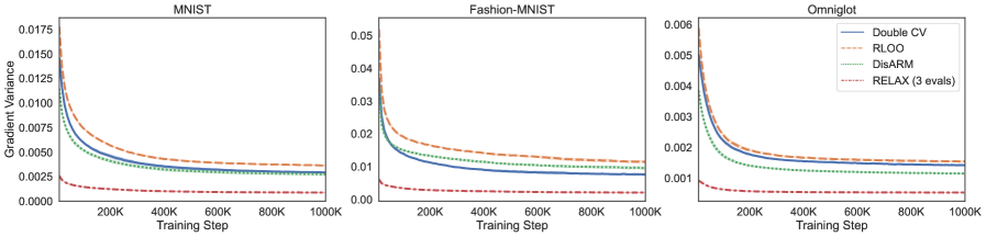
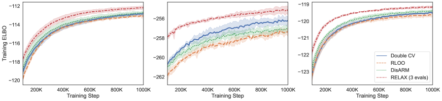
Figure 9: Training linear binary latent VAEs with Bernoulli likelihoods with $K=2$ (except RELAX which needs 3 evaluations of $f$) on dynamically binarized MNIST, Fashion-MNIST, and Omniglot. Top: Variance of gradient estimates. Bottom: Average ELBO on training examples.

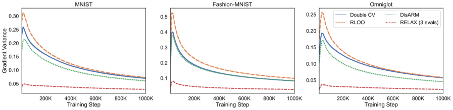
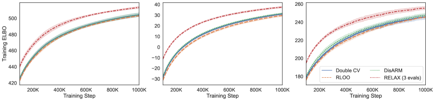
Figure 10: Training linear binary latent VAEs with Gaussian likelihoods with $K=2$ (except RELAX which needs 3 evaluations of $f$) on non-binarized MNIST, Fashion-MNIST, and Omniglot. Top: Variance of gradient estimates. Bottom: Average ELBO on training examples.

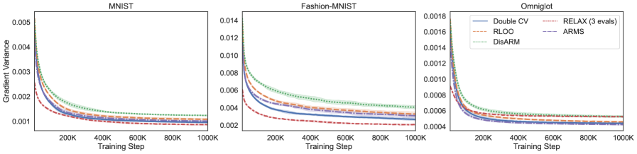
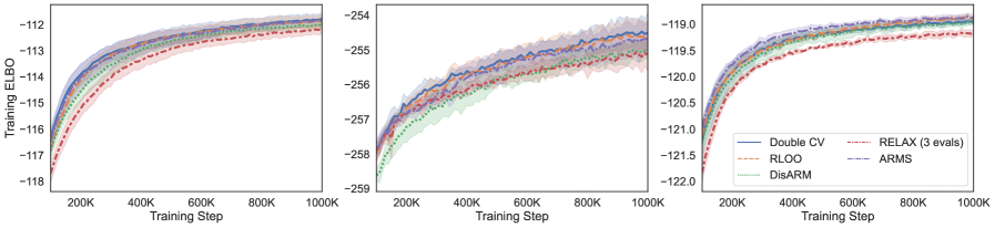
Figure 11: Training linear binary latent VAEs with Bernoulli likelihoods with $K=4$ (except RELAX which needs 3 evaluations of $f$) on dynamically binarized MNIST, Fashion-MNIST, and Omniglot. Top: Variance of gradient estimates. Bottom: Average ELBO on training examples.

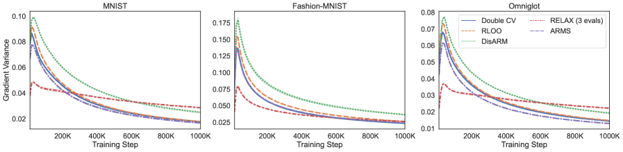
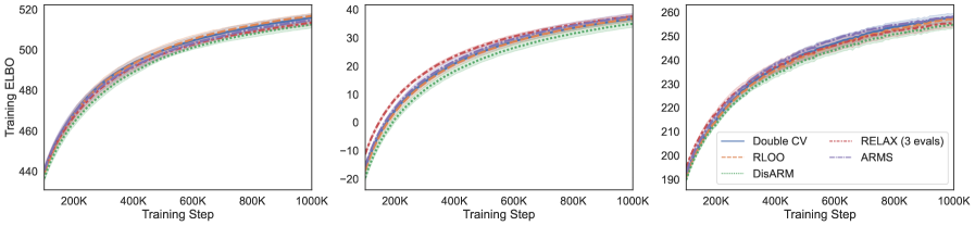
Figure 12: Training linear binary latent VAEs with Gaussian likelihoods with $K=4$ (except RELAX which needs 3 evaluations of $f$) on non-binarized MNIST, Fashion-MNIST, and Omniglot. Top: Variance of gradient estimates. Bottom: Average ELBO on training examples.

References

• Blei et al., (2017) Blei, D. M., Kucukelbir, A., and McAuliffe, J. D. (2017). Variational inference: A review for statisticians. Journal of the American statistical Association, 112(518):859–877.
• Carbonetto et al., (2009) Carbonetto, P., King, M., and Hamze, F. (2009). A stochastic approximation method for inference in probabilistic graphical models. In Advances in Neural Information Processing Systems, volume 22.
• Dimitriev and Zhou, (2021) Dimitriev, A. and Zhou, M. (2021). ARMS: antithetic-reinforce-multi-sample gradient for binary variables. In International Conference on Machine Learning, volume 139, pages 2717–2727.
• Dong et al., (2020) Dong, Z., Mnih, A., and Tucker, G. (2020). DisARM: An antithetic gradient estimator for binary latent variables. In Advances in Neural Information Processing Systems, volume 33, pages 18637–18647. Curran Associates, Inc.
• Dong et al., (2021) Dong, Z., Mnih, A., and Tucker, G. (2021). Coupled gradient estimators for discrete latent variables. arXiv preprint arXiv:2106.08056.
• Geffner and Domke, (2018) Geffner, T. and Domke, J. (2018). Using large ensembles of control variates for variational inference. In Advances in Neural Information Processing Systems, volume 31.
• Glasserman, (2003) Glasserman, P. (2003). Monte Carlo methods in financial engineering, volume 53. Springer Science & Business Media.
• Glynn, (1990) Glynn, P. W. (1990). Likelihood ratio gradient estimation for stochastic systems. Commun. ACM, 33(10):75–84.
• Grathwohl et al., (2018) Grathwohl, W., Choi, D., Wu, Y., Roeder, G., and Duvenaud, D. (2018). Backpropagation through the void: Optimizing control variates for black-box gradient estimation. In International Conference on Learning Representations.
• Gu et al., (2016) Gu, S., Levine, S., Sutskever, I., and Mnih, A. (2016). MuProp: Unbiased backpropagation for stochastic neural networks. In International Conference on Learning Representations.
• Kingma and Ba, (2014) Kingma, D. P. and Ba, J. (2014). Adam: A method for stochastic optimization. International Conference for Learning Representations.
• Kingma and Welling, (2014) Kingma, D. P. and Welling, M. (2014). Auto-encoding variational Bayes. In International Conference on Learning Representations.
• Kool et al., (2019) Kool, W., Hoof, H. V., and Welling, M. (2019). Buy 4 reinforce samples, get a baseline for free! In DeepRLStructPred@ICLR.
• Mnih and Gregor, (2014) Mnih, A. and Gregor, K. (2014). Neural variational inference and learning in belief networks. In International Conference on Machine Learning, pages 1791–1799.
• Mnih and Rezende, (2016) Mnih, A. and Rezende, D. J. (2016). Variational inference for Monte Carlo objectives. In International Conference on Machine Learning.
• Owen, (2013) Owen, A. B. (2013). Monte Carlo theory, methods and examples.
• Paisley et al., (2012) Paisley, J. W., Blei, D. M., and Jordan, M. I. (2012). Variational Bayesian inference with stochastic search. In International Conference on Machine Learning.
• Ranganath et al., (2014) Ranganath, R., Gerrish, S., and Blei, D. (2014). Black box variational inference. In International Conference on Artificial Intelligence and Statistics, page 814–822.
• Rezende et al., (2014) Rezende, D. J., Mohamed, S., and Wierstra, D. (2014). Stochastic backpropagation and approximate inference in deep generative models. In International Conference on Machine Learning.
• Richter et al., (2020) Richter, L., Boustati, A., Nüsken, N., Ruiz, F., and Akyildiz, O. D. (2020). VarGrad: A low-variance gradient estimator for variational inference. In Advances in Neural Information Processing Systems, volume 33, pages 13481–13492. Curran Associates, Inc.
• Robbins and Monro, (1951) Robbins, H. and Monro, S. (1951). A Stochastic Approximation Method. The Annals of Mathematical Statistics, 22(3):400–407.
• Salimans and Knowles, (2014) Salimans, T. and Knowles, D. A. (2014). On using control variates with stochastic approximation for variational Bayes and its connection to stochastic linear regression. arXiv preprint arXiv:1401.1022.
• Titsias and Lázaro-Gredilla, (2014) Titsias, M. K. and Lázaro-Gredilla, M. (2014). Doubly stochastic variational Bayes for non-conjugate inference. In International Conference on Machine Learning.
• Titsias and Lázaro-Gredilla, (2015) Titsias, M. K. and Lázaro-Gredilla, M. (2015). Local expectation gradients for black box variational inference. Advances in Neural Information Processing Systems, 28:2638–2646.
• Tokui and Sato, (2017) Tokui, S. and Sato, I. (2017). Evaluating the variance of likelihood-ratio gradient estimators. In International Conference on Machine Learning, pages 3414–3423.
• Tucker et al., (2017) Tucker, G., Mnih, A., Maddison, C. J., and Sohl-Dickstein, J. (2017). REBAR: low-variance, unbiased gradient estimates for discrete latent variable models. In International Conference on Learning Representations.
• Weaver and Tao, (2001) Weaver, L. and Tao, N. (2001). The optimal reward baseline for gradient-based reinforcement learning. In Uncertainty in Artificial Intelligence, pages 538–545.
• Williams, (1992) Williams, R. J. (1992). Simple statistical gradient-following algorithms for connectionist reinforcement learning. Machine Learning, 8(3-4):229–256.
• Yin et al., (2020) Yin, M., Ho, N., Yan, B., Qian, X., and Zhou, M. (2020). Probabilistic best subset selection via gradient-based optimization.
• Yin and Zhou, (2019) Yin, M. and Zhou, M. (2019). ARM: Augment-REINFORCE-merge gradient for stochastic binary networks. In International Conference on Learning Representations.