On the band-width of stable nonlinear stripe patterns in finite size systems

Abstract

Nonlinear stripe patterns occur in many different systems, from the small scales of biological cells to geological scales as cloud patterns. They all share the universal property of being stable at different wavenumbers $q$, i.e., they are multistable. The stable wavenumber range of the stripe patterns, which is limited by the Eckhaus- and zigzag instabilities even in finite systems for several boundary conditions, increases with decreasing system size. This enlargement comes about because suppressing degrees of freedom from the two instabilities goes along with the system reduction, and the enlargement depends on the boundary conditions, as we show analytically and numerically with the generic Swift-Hohenberg (SH) model and the universal Newell-Whitehead-Segel equation. We also describe how, in very small system sizes, any periodic pattern that emerges from the basic state is simultaneously stable in certain parameter ranges, which is especially important for Turing pattern in cells. In addition, we explain why below a certain system width stripe pattern behave quasi-one-dimensional in two-dimensional systems. Furthermore, we show with numerical simulations of the SH model in medium-sized rectangular domains how unstable stripe patterns evolve via the zigzag instability differently into stable patterns for different combinations of boundary conditions.

Nonlinear stripe patterns are ubiquitous in nature, and their driving mechanisms are as diverse as the systems themselves in which they occur CrossHo ; Ball:98 ; Busse:78.1 ; Kramer:96 ; Aranson:02.1 ; Kapral:1995 ; BoPeAh:2000.1 ; Mikhailov:2006.1 ; Pismen:2006 ; Kondo_Miura:2010.1 ; Lappa:2010 ; Sasai:2013.1 ; Meron:2015 ; Meron:2018.1 ; BaerM:2020.1 . Stripe patterns have the universal property of being stable at different values of the wavenumber, and these stable wavenumber regions are the so-called Busse balloons after their pioneer Busse:1967.2 ; Busse:78.1 ; CrossHo ; Newell:1993.1 ; Lappa:2010 . To the instabilities bounding the stable wavenumber range of stripe patterns count the generic Eckhaus instability , a long-wavelength longitudinal (compressional) instability, and the zigzag instability, a long-wavelength transverse instability Newell:1969.1 ; CrossHo . Stable wavenumber ranges are restricted even in large systems by pattern suppressing boundary conditions at the domain sides CDHS ; Kramer:1984.1 or are even selected by spatial inhomogeneities, e.g. via so-called ramps Kramer:82.1 ; Ahlers:83.1 ; Cross:1984.1 . In contrast, in short systems the stable wavenumber range can be enlarged, as in Ref. Zimmermann:85.1 for quasi-one-dimensional systems predicted and experimentally confirmed in Ref. Ahlers:86.1 ; Dominguez-Lerma:86.2 . Such a range extension depends on the boundary conditions and the second spatial dimension as we explain in this work analytically and numerically by investigating the generic Swift-Hohenberg model and the universal Newell-Whitehead-Segel equation in rectangular domains. Finite size effects on patterns are also highly relevant for Turing patterns in small systems, as for instance in cells deBoer:1999.1 ; DekkerC:2015.1 ; Sourjik:2017.1 ; Bergmann:2018.1 .

I Introduction

Patterns occur spontaneously in a plethora of living or inanimate driven systems, such as in the atmosphere or in convection cells, in biological cells, in chemical reactions, or as vegetation patterns, to name just a few examples CrossHo ; Ball:98 ; Busse:78.1 ; Kramer:96 ; Aranson:02.1 ; Kapral:1995 ; BoPeAh:2000.1 ; Mikhailov:2006.1 ; Pismen:2006 ; Kondo_Miura:2010.1 ; Lappa:2010 ; Sasai:2013.1 ; Meron:2015 ; Meron:2018.1 ; BaerM:2020.1 . Already the esthetic appeal of patterns is immediately apparent to all observers Ball:98 . Patterns fulfill also important functions in nature. For example, self-organized patterns in biology guide size sensing LanderAD:2011.1 , positioning of protein clusters in the cell center in advance of cell division Sourjik:2017.1 or in self-driven morphogenesis Sasai:2013.1 . Patterns enhance transport in fluid systems CrossHo ; Lappa:2010 or they are the basis of successful survival strategies for vegetation in water-limited systems Meron:2015 ; Meron:2018.1 .

Patterns are multistable, i.e. they are stable for different wavenumbers within a stability band CrossHo ; Newell:1969.1 ; Busse:78.1 , sometimes also beyond a seondary instability ThomsenF:2021.1 . In quasi-one-dimensional systems, the stability band is bounded by the Eckhaus instability Eckhaus:65 ; Newell:1969.1 ; CrossHo ; Boucif:84.1 ; Zimmermann:85.1 ; Ahlers:86.1 ; Dominguez-Lerma:86.2 ; Riecke:86.1 ; Lowe:85.2 ; Zimmermann:85.3 ; Dominguez-Lerma:86.1 ; Zimmermann:88.1 ; Tuckerman:1990.1 , which also has its two-dimensional generalization in anisotropic systems Kramer:1986.1 ; Zimmermann:88.3 . In two-dimensional isotropic systems, the stability band of stripe patterns is in addition bounded by the zigzag instability Newell:1969.1 ; CrossHo ; Cross:2009 .

In nature, patterns are always exposed to boundaries, be it the walls of a convection cell, the finite size of a Petri dish, or the cytosol bounding membrane for intracellular processes. Along these boundaries, the fields describing the patterns must satisfy certain boundary conditions. Some boundary conditions suppress the pattern near the boundary. In longitudinal direction they act even in long sytems far into the volume and significantly restrict the stable wavenumber band CDHS . In contrast, periodic and no-flux boundary conditions, for example, impose no restriction on the stable wavenumber band, except that the wavenumbers can take only discrete values. In rectangular systems with amplitude-suppressing boundary conditions, stripe patterns prefer an orientation perpendicular to these edges Greenside:84.1 ; CrossHo ; Ruppert:2020.1 .

Patterns are also restricted to finite ranges when the control parameter generating a pattern falls to subcritical values outside a subrange. Examples include photosensitive chemical reactions. There, pattern formation can be suppressed by illuminating the reaction cell outside a finite range Epstein:1999.1 or even controlled by spatially modulated illumination Epstein:2001.1 ; PeterR:2005.1 ; Hammele:2006.2 . Another example is protein patterns occurring in finite reactive subdomains of substrates Schwille:2012.1 . In such examples, orientations are often perpendicular to non-resonant control parameter drops Rapp:2016.1 ; Ruppert:2020.1 . In the case of steep control parameter decays, stationary strips may orient parallel to the boundaries due to resonance effects Rapp:2016.1 . In quasi-one-dimensional systems, spatial variations, called ramps, break the translational symmetry and drastically reduce the width of the stable wavenumber band Kramer:82.1 ; Ahlers:83.1 ; Cross:1984.1 ; Kramer:1985.1 ; Riecke:86.1 .

No-flux boundary conditions play a central role for reaction-diffusion patterns in cells and elsewhere. No-flux boundary conditions break translational symmetry and fix the phase of a periodic pattern at the boundary, but they share the property of leaving the threshold untouched and, in medium sized systems, also the stable wavenumber band. Both boundary conditions are very well suited to study the direct influence of the system size on the stability range of striped patterns. From investigations on quasi one-dimensional systems it is known that a decrease of the system size leads to an increase of the Eckhaus stable wavenumber band Zimmermann:85.1 , which is also confirmed experimentally Ahlers:86.1 ; Dominguez-Lerma:86.2 . This is an opposite trend as obtained for medium sized and long systems with amplitude suppressing boundary conditions in longitudinal direction and for ramps.

Therefore, an interesting question arises: how will the zigzag instability boundary of the stable wavenumber band be shifted by reducing the size of the domain containing the patterns? We address this question by studying the stability of stripe solutions of the Swift-Hohenberg model in rectangular domains as well as and simultaneously with the universal Newell-Whitehead-Segel equation. Since in rectangular domains stripe patterns are oriented perpendicular to edges with amplitude suppressing conditions, we choose either periodic or no-flux boundary conditions along the short sides of the rectangle and combine them with these two boundary conditions also along the long sides of the rectangle. This allows us to analytically determine the Eckhaus stability boundary and the zigzag stability boundary in section III. Combining these boundary combinations gives very good analytical estimates of the shifts of the Eckhaus and zigzag stability boundary with decreasing system size, for several boundary conditions along the transverse direction. This is also checked numerically in section IV. There we also compare the analytical results on the instability limits with numerical results for the case when amplitude-suppressing boundary conditions are used in the transverse direction.

The results in section ,III describe that in small systems one finds remarkable broadenings of the stable wavenumber band by reducing the system size. Also, stripes in two spatial dimensions behave quasi-one-dimensional in rather narrow systems. In contrast, the evolution of a stripe pattern from an unstable to a stable wavenumber already in medium-size systems depends significantly on the nature of the boundary conditions, as we show with exemplary simulations in Sec. V. A summary and conclusions are given in section VI.

II Models

Generic properties of stripe patterns just above threshold can be described by models such as the isotropic Swift-Hohenberg (SH) model Hohenberg:1977.1 ; CrossHo ; Cross:2009 . It contains the characteristic wavenumber $q_{0}$ of the pattern and allows in two spatial dimensions also the modeling of spatial variations of the local wavevector of periodic patterns. Essential universal properties of periodic patterns are also captured by the dynamics of the pattern envelope varying slowly on the wavelength of the pattern.Newell:1969.1 ; CrossHo ; Cross:2009 . The dynamical equation for the envelope in isotropic systems is described by the so-called universal Newell-White-Segel equation (NWSE) Newell:1969.1 ; Segel:69.1 ; Newell:1993.1 ; CrossHo ; Cross:2009 , which can be derived from the SH model as well CrossHo . We use here both complementary model descriptions of stripe patterns.

II.1 Swift-Hohenberg model

The rotational invariant Swift-Hohenberg model for the scalar field $u({\bf r},t)$ above supercritical bifurcations isHohenberg:1977.1 ; CrossHo ; Cross:2009 ,

$$\partial_{t}u=\varepsilon u-(q_{0}^{2}+\nabla^{2})^{2}u-u^{3}\,,$$ (1)

with the control parameter $\varepsilon$ and the intrinsic wavenumber $q_{0}$. Near the threshold of periodic patterns ($\varepsilon_{c}=0$) the solutions of the SH-model can be also expressed in terms of a slowly varying amplitude $A(x,y,t)$ as follows:

$$u(x,y,t)=A(x,y,t)e^{iq_{0}x}+A^{\ast}(x,y,t)e^{-iq_{0}x}+h.o.t.\,.$$ (2)

II.2 Newell-Whitehead-Segel equation

The dynamical equation for the patterns envelope $A(x,y,t)$ can be derived from the SH model as well as other pattern forming systems, such as from the basic equation of thermal convection in liquids. Through a systematic multiscale perturbations analysis around the onset of periodic patterns and using the property that the envelope $A(x,y,t)$ varies slowly on the scale of a wavelength of the pattern, $2\pi/q_{0}$, Newell:1969.1 ; Segel:69.1 ; Newell:1993.1 ; CrossHo ; Cross:2009 one obtains the so-called Newell-Whitehead-Segel equation (NWSE) for the amplitude $A(x,y,t)$:

$$\tau_{0}\partial_{t}A=\varepsilon A+\xi_{0}^{2}(\partial_{x}-\frac{i}{2q_{0}}\partial_{y}^{2})^{2}A-g_{0}|A|^{2}A\,.$$ (3)

The systems specific properties are covered by the coefficients, i.e. the values and their meanings depend on the system but the form of the NWSE is universal. If Eq. (3) is derived from the SH equation Eq. (1) one obtains $\tau_{0}=1$, $\xi_{0}=2q_{0}$ and $g_{0}=3$. The universal NWSE with the coefficients corresponding to the SH model reproduces stability ranges of stripe pattern near the threshold as well, as exemplarily shown in Appendix A.4.

II.3 Boundary conditions

Here, the nonlinear stripe patterns are investigated in rectangular areas with respect to four different boundary conditions. One type are periodic boundary conditions (PBC)

$$u(x=0,y) =u(x=L_{x},y)\,,\qquad\quad(\mbox{x-PBC})~{}\,$$ (4)

$$u(x,y=0) =u(x,y=L_{y})\,.\qquad\quad~{}(\mbox{y-PBC})\,$$ (5)

PBC take just into account finite-size effects and the possible wavelengths can take only discrete values. We also consider Neumann boundary conditions, which are also known as no-flux boundary conditions:

$$(\vec{n}\cdot\nabla)u=0=(\vec{n}\cdot\nabla)^{3}u\,.\qquad(\mbox{BCI})\,$$ (6)

Vanishing amplitude and curvature normal to the rectangular boundary is implemented by he third type of boundary conditions considered here:

$$u=0=(\vec{n}\cdot\nabla)^{2}u\,.\qquad\qquad~{}~{}(\mbox{BCII})\,$$ (7)

The fourth type of boundary conditions for the field $u(x,y,t)$,

$$\left.u(x,y)\right|_{y=0,L_{y}}=0=\partial_{y}\left.u(x,y)\right|_{y=0,L_{y}}\,\qquad(\mbox{BCIII})$$ (8)

is only used here along the long sides at $y=0,L_{y}$. These boundary conditions are suitable for example for stripe patterns in thermal convection in finite boxes, to model so-called no-slip boundary conditions for the flow velocity. Effects of the boundary conditions BCIII in both directions in a two-dimensional systems are investigated for the SH model also in Ref. Greenside:84.1 .

II.4 Stationary single-mode solutions of the SH model

Perturbations $u=\bar{u}\exp(\sigma t+i{\bf q}\cdot{\bf r})$ with ${\bf q}=(q,p)$ of the basic state $u=0$ of the SH equation grow beyond the so-called neutral curve

$$\varepsilon_{0}(q_{n},p_{m})=(q_{0}^{2}-q_{n}^{2}-p_{m}^{2})^{2}\,.$$ (9)

Note, that in finite systems only discrete values $q_{n}$ and $p_{m}$ match into the system for the boundary conditions PBC, BCI and BCII. For PBC one has $q_{n}=n2\pi/L_{x}$ and $p_{m}=m2\pi/L_{y}$. For BCI and BCII the discretization steps are half the size: $q_{n}=n\pi/L_{x}$ and $p_{m}=m\pi/L_{y}$. Consider stripe perturbations with periodicity in the $x$-direction and taking into account the boundary conditions one has:

$$u =\bar{u}\exp(\sigma t)\cos(q_{n}x)\,,\qquad\mbox{(BCI)}$$

$$u =\bar{u}\exp(\sigma t)\sin(q_{n}x)\,.\qquad\mbox{(BCII)}$$ (10)

The growth rate vanishes along $\varepsilon_{0}$ and beyond $\varepsilon_{0}(q)$ the perturbations grow up to a saturation amplitude.

With $\sigma=0$ and $\bar{u}=2A_{s}$ in Eq. (II.4) and for PBC or BCI in the $y$-direction one obtains after projection of the SH equation (1) onto $\cos(q_{n}x+\varphi)$ with $\varphi=0$ for BCI, $\varphi=\pi/2$ for BCII and arbitrary $\varphi$ for PBC in the $x$-direction the expression for the following amplitude of stripes:

$$A_{s}^{2}=\left[\varepsilon-(q_{0}^{2}-q_{n}^{2})^{2}\right]/3\,.$$ (11)

The determination of the threshold and the amplitude in the case of BCIII requires essentially a numerical approach as in Ref.Greenside:84.1 and the onset of the periodic pattern takes place at higher values of $\varepsilon$. In the case of BCII in the $y$-direction and the stripe axis parallel to $y$ the nonlinear solution has to be determined numerically as well.

III Stability boundaries of stripes

The linear stability of stripe solutions of the SH model in rectangular domains can be studied analytically for periodic boundary conditions in Eq. (4), the no-flux boundary conditions Eq. (6) and for BCII-type boundary conditions in Eq. (7). This is described in this section and also includes the analytical determination of the Eckhaus stability boundary of stripe solutions as well as the zigzag stability boundary for stripes. Solutions of the Newell-Whitehead-Segel equation and their stability are delineated in Appendix A.1 including a comparison with the following results obtained for the SH model.

III.1 The zigzag instability for the SH model

To investigate the zigzag instability we add a small perturbation $v(x,y,t)$ to the stripe solution $u_{0}=A_{s}\exp(iq_{n}x)+cc$: $u=u_{0}+v$. A linearization of Eq. (1) with respect to $v$ gives the linear equation,

$$\partial_{t}v=[\varepsilon-(q_{0}^{2}+\nabla^{2})^{2}-3u_{0}^{2}]v+{\cal O}(v^{2})\,.$$ (12)

It is solved analytically by the ansatz

$$v =e^{\sigma t}\cos(q_{n}x+\varphi)\left(e^{ip_{j}y}v_{1}+e^{-ip_{j}y}v_{2}\right)$$ (13)

with discrete wavenumbers $q_{n}$ and the following boundary types in the $x$-direction, PBC, BCI ($\varphi=0)$ and BCII ($\varphi=\pi/2$) and discrete values $p_{j}$ in the $y$-direction for PBC and BCI boundary conditions . The only difference for the boundary conditions are the allowed discrete values of $q_{n}$ and $p_{j}$. These are $q_{n}=n\pi/L_{x}$ for BCI, BCII and $q_{n}=2n\pi/L_{x}$ for PBC in the $x$-direction and analogously in the $y$-direction for BCI $p_{j}=j\pi/L_{y}$ and for PBC $p_{j}=j2\pi/L_{y}$. The result contradicts the recent claim in Ref.Yochelis:2020.1 that the ansatz for the zigzag instability in Eq. (13) does not hold in the case of no-flux boundary conditions in the $x$-direction. Moreover, in Ref. Yochelis:2020.1 it was claimed, that the perturbation $v(x,y,t)$ must become small near $x=0,L_{x}$, which is definitely not imposed by no-flux boundary conditions BCI.

Collecting the linear independent contributions $\propto e^{i(q_{n}x\pm p_{j}y)}$ in Eq. (12) gives two coupled homogeneous equations for $v_{1}$ and $v_{2}$ with the solubility condition

$$\begin{vmatrix}{\cal L}-6A_{s}^{2}\qquad&-3A_{s}^{2}~{}~{}\\ -3A_{s}^{2}~{}~{}~{}&{\cal L}-6A_{s}^{2}\end{vmatrix}=0\,,$$ (14)

where the linear operator ${\cal L}$ is given by

$${\cal L}=\varepsilon-\sigma-(q_{0}^{2}-q_{n}^{2}-p_{j}^{2})^{2}\,.$$ (15)

With the stationary amplitude $A_{s}(q_{n})$ from Eq. (11) the growth rate takes the following form:

$$\sigma=p_{j}^{2}\left[2\left(q_{0}^{2}-q_{n}^{2}\right)-p_{j}^{2}\right]\,.$$ (16)

For a nonlinear periodic solution of wavenumber $q_{n}$ this growth rate $\sigma$ of the perturbation $v$ with the transversal wavenumber $p_{j}$ becomes positive when the wavenumber $q_{n}$ becomes smaller than $q_{zz}$ at the zigzag stability boundary:

$$q_{n}<q_{\text{zz}}=\sqrt{q_{0}^{2}-\frac{p_{j}^{2}}{2}}\,.$$ (17)

The shift of $q_{zz}$ to a value smaller than $q_{0}$ is determined by the smallest perturbation wavenumber $p_{1}$ that matches into the interval $[0,L_{y}]$. $p_{1}$ is two times larger for periodic boundary conditions and therefore the shift of $q_{zz}$ away from $q_{0}$ is larger in the case of periodic boundary conditions, compared to BCI. This also means that the stable $q$ range for stripes is stronger enhanced for PBC than for BCI as shown in Fig. 1 below.

III.2 Finite size effects on the Eckhaus instability

The determination of the stability of periodic patterns against longitudinal perturbations gives the so-called Eckhaus-boundary stability boundary and for this a one-dimensional analysis of Eq. (12) is sufficient. In simulations one can achieve a quasi one-dimensional behavior of stripe patterns by choosing in simulations a small extension $L_{y}$ (see also Sec. IV). Therefore, we choose a one-dimensional ansatz $v(x,t)$ for Eq. (12):

$$v=e^{\sigma t}\left[e^{iq_{n}x}\left(e^{ik_{j}x}v_{1}+e^{-ik_{j}x}v_{2}^{\ast}\right)+cc\right]\,.$$ (18)

In finite systems also the wavenumber $k_{j}$ of the perturbation is limited to discrete values. For boundary conditions BCI and BCII along $x$ one has $k_{j}=j\pi/L_{x}$ and for periodic boundary conditions one has $k_{j}=j2\pi/L_{x}$. Also the longitudinal instability is a along wavelength instability, i.e. growth rate becomes at first positive at the smallest perturbation wavenumber $k_{1}$. If the perturbation $v$ is growing with a wavenumber $k_{1}$, then during the instability process either a node is added to the stripe solution or removed. By using the ansatz (18) in Eq. (12) and collecting the contributions $\propto e^{i(q_{n}\pm k_{1})x}$ one obtains two coupled homogeneous equations for $v_{1}$ and $v_{2}$ with the solubility condition

$$\begin{vmatrix}{\cal L}_{+}-\sigma\qquad&-3A_{s}^{2}~{}~{}\\ -3A_{s}^{2}~{}~{}~{}&{\cal L}_{-}-\sigma\end{vmatrix}=0.$$ (19)

and the abbreviation

$${\cal L}_{\pm} =-\varepsilon+\underbrace{2(q_{0}^{2}-q_{n}^{2})^{2}-(q_{0}^{2}-(q_{n}\pm k_{1})^{2})^{2}}_{M_{\pm}}\,.$$ (20)

The growth rate of the perturbation expressed in terms of ${\cal L}_{\pm}$ is given by

$$\sigma =\frac{1}{2}\left({\cal L}_{+}+{\cal L}_{-}+\sqrt{({\cal L}_{+}-{\cal L}_{-})^{2}+36A_{s}^{4}}\right)\,.$$ (21)

The neutral stability condition $\sigma=0$ for periodic solution of wavenumber $q_{n}$ is given by

$$({\cal L}_{+}+{\cal L}_{-})^{2} =({\cal L}_{+}-{\cal L}_{-})^{2}+36A_{s}^{4}$$ (22)

or in different form by

$${\cal L}_{+}{\cal L}_{-} =9A_{s}^{4}\,.$$ (23)

This gives the control parameter value $\varepsilon(q_{n})=\varepsilon_{n}$ at the neutral stability of a stripe pattern of wavenumber $q_{n}$

$$\varepsilon(q_{n})=\varepsilon_{n}=\frac{M_{+}M_{-}-(q_{0}^{2}-q_{n}^{2})^{4}}{M_{+}+M_{-}-2(q_{0}^{2}-q_{n}^{2})^{2}}\,.$$ (24)

For $\varepsilon>\varepsilon_{n}$ the periodic solution is stable and below in the range $\varepsilon_{0}(q_{n})<\varepsilon<\varepsilon_{n}$ linear unstable with respect to the longitudinal perturbation of wavenumber $k_{1}$.

IV Linear stability diagrams of stripes

Stability diagrams of stripe patterns with their wavevector ${\bf q}=(q,0)$ along the $x$ axis are presented in this section. The position of the zigzag-stability boundary, $q_{zz}$, and the Eckhaus-stability boundary (E) of stripe patterns in a rectangular domain are shown in Fig. 1 for two widths $L_{y}$, in the $y$-direction either periodic (PBC) or no-flux boundary conditions (BCI) and no-flux boundary conditions at $x=0,L_{x}$. The solid line N in Fig. 1 is the neutral curve described by Eq. (9).

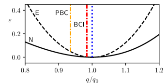
Figure 1: Shown is the neutral curve (solid line), the Eckhaus-stability boundary (dashed line) and the vertical lines mark the zigzag instability $q_{zz}$ given by Eq. (17) for different $L_{y}$ and for BCI and PBC in the $y$-direction. The vertical dotted line marks $q_{zz}$ for both, BCI and PBC at $L_{y}=40\lambda_{0}$. For $L_{y}=2\lambda_{0}$ the position of $q_{zz}$ is stronger shifted for PBC (left dash-dotted line) than for BCI (right dash-dotted line).

The vertical dotted line in Fig. 1 marks the position of the zigzag-stability boundaries $q_{zz}$ obtained via Eq. (17) for a broad rectangle with $L_{y}=40\lambda_{0}$ and for BCI and PBC at $y=0,L_{y}$. The $q_{zz}$ for both cases is indistinguishable. In a narrow system with $L_{y}=2\lambda_{0}$ the zigzag-stability boundary for PBC in the $y$-direction in Fig. 1 is about four times as far shifted to the left than for BCI. The reason, the smallest wavenumber of a perturbation of the periodic stripe solution in a system of width $L_{y}$ is for PBC twice as large as for BCI, i.e., $p_{1}^{PBC}=2p_{1}^{BCI}$ and its square $p_{1}^{2}$ contributes to $q_{zz}$ in Eq. (17). Thus, the location of the zigzag stability boundary depends essentially on the system extent $L_{y}$ and on the boundary conditions in the $y$-direction of the stripe axis, but not on the boundary conditions perpendicular to the stripe wavevector in the $x$-direction.

In one-dimensional systems with large $L_{x}$ the Eckhaus-stability boundaries (ESB) for BCI and PBC in the $x$-direction are indistinguishable and given by the dashed line in Fig. 2.

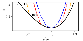
Figure 2: Shown is the ESB in the one-dimensional case for both, PBC and BCI in the $x$-direction. In a long system with $L_{x}=40\lambda_{0}$ the ESB’s are indistinguishable for PBC and BCI (dashed line). In a short system with $L_{x}=2\lambda_{0}$ (dash-dotted lines) the Eckhaus stability range is broader for PBC than for BCI. The solid line N is the neutral curve.

The location of the ESB depends on the length $L_{x}$ and also on boundary conditions in the $x$-direction. To illustrate this, we show in Fig. 2 also the Eckhaus boundary for a short system with only two periodic pattern units in the system. For this purpose, we consider the case of a pattern of wavenumber $q$ in a system of suitable length $L_{x}=2(2\pi/q)$ for the two boundary conditions PBC and BCI at $x=0,L_{x}$. The ESB is determined by Eq. (24), but with $k_{1}=\pi/L_{x}$ for BCI and $k_{1}=2\pi/L_{x}$ for PBC. For both short systems, the ESB intersects the neutral curve, as shown in Fig. 2. For $\varepsilon$ below this intersection the periodic patterns are stable for all $q$ between neutral curve, i.e. for all stripe patterns that emerge. The dependence of the Eckhaus boundary on the system length was already recognized in Ref. Zimmermann:85.1 and this length dependence was also confirmed in experiments on Taylor vortex flow in Ref. Dominguez-Lerma:86.2 . The ESB is similar as for the zigzag boundary for PBC shifted further from the Eckhaus boundary for very long systems than for the boundary condition BCI. The difference is again caused by the different value of the perturbations wavenumber, similar as for the zigzag instability.

The wavenumber along the Eckhaus curve, as for example along the dashed curve in Fig. 2, we call $q_{E}(\varepsilon)$. Its deviation from the preferred wavenumber $q_{0}$ is $Q_{E}=q_{E}-q_{0}$. Defining analogous $q_{N}(\varepsilon)$ as the wavenumber along the neutral curve and its deviation from the preferred wavenumber $Q_{N}=q_{N}-q_{0}$, the ratio between both deviations follow near the threshold ($\varepsilon\ll 1$) the universal law of stripe patterns in one spatial dimension Newell:1969.1 ; Zimmermann:85.1 ; Cross:2009 :

$$\frac{Q_{E}}{Q_{N}}=\frac{1}{\sqrt{3}}\,.$$ (25)

The ratio becomes larger in systems of finite extension $L_{x}$. In addition, the ratio depends on $\varepsilon$, $L_{x}$ and on the boundary conditions in the longitudinal $x$-direction.

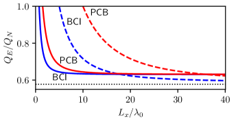
Figure 3: Shown is the ratio $Q_{E}/Q_{N}$ between the half-width of the Eckhaus-stability band, $Q_{E}$, and the half-width of the neutral curve, $Q_{N}$, as function of the system length $L_{x}/\lambda_{0}$ for the two boundary conditions PBC and BCI and for the control parameter $\varepsilon=0.01$ (dashed lines) and $\varepsilon=0.4$ (solid curves).

We determine via Eq. (24) the wavevector along the Eckhaus boundary, $q_{E}(\varepsilon,k_{1})$, as function of $\varepsilon$ with $k_{1}=\pi/L_{x}$ for BCI (resp. $k_{1}=2\pi/L_{x}$ for PBC). The ratio between $Q_{E}(\varepsilon,k_{1})$ and $Q_{N}=q_{N}-q_{0}$ is shown for the SH model in Fig. 3 as function of $L_{x}$ for two different values of $\varepsilon$ and two boundary conditions. For an infinite system near threshold this ratio is given by Eq. (25), which is indicated by the dotted horizontal line in Fig. 3. For PBC the ESB is shifted further away from the value for infinite systems in Eq. (25) and closer to the neutral curve $\varepsilon_{0}(q)$ than for BCI. This means the ESB reaches the neutral curve (see also Fig. 2) and thus the largest possible value $Q_{E}/Q_{N}=1$ for a chosen $\varepsilon$ already at larger system lengths $L_{x}$ than for no-flux boundary conditions BCI.

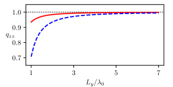
Figure 4: The zigzag stability boarder $q_{zz}$, given by Eq. (17), is shown as a function of the system width $L_{y}$ for no-flux boundary conditions (BCI) (solid line) and for periodic boundary conditions (dashed line) in the $y$-direction.

The value $q_{zz}$ at the $\varepsilon$-independent zigzag-stability boundary has different values for different boundary conditions in the $y$-direction as indicated in Fig. 1. The dependence of $q_{zz}$ on the system width $L_{y}$ is shown in Fig. 4 for the two boundary conditions PBC and BCI in the $y$-direction. $q_{zz}$ decreases with decreasing $L_{y}$ in both cases, but stronger for PBC. The reason is again the larger perturbation wavenumber $k_{1}$ in Eq. (20) for PBC.

A consequence of the $L_{y}$ dependence of $q_{zz}$ in Fig. 4 is further illustrated in Fig. 5. Shown is the neutral cuve (dashed-dotted), the Eckhaus boundary (solid line) and the zigzag instability for the two lateral extensions $L_{y}=2\lambda_{0},~{}1.5\lambda_{0}$ and three different boundary conditions in the $y$-direction. For the wider system with $L_{y}=2\lambda_{0}$ the zigzag instability $q_{zz}$ for BCII ($+$ symbols) is located between $q_{zz}$ for BCI (vertical solid line) and $q_{zz}$ for PBC (vertical dashed line). Also for the narrower system with $L_{y}=1.5\lambda_{0}$ the zigzag instability $q_{zz}$ for the type BCII boundary condition ($\times$ symbols) is between $q_{zz}$ for BCI boundary conditions (vertical dashed-dotted line) and $q_{zz}$ for PBC (dashed-dot-dotted line). While the results for BCI and PBC are determined by the expression in Eq. (17), the zigzag instability for y-BCII are determined via simulations. In this sense the analytical formula of $q_{zz}$ for BCI and PBC gives a reasonable estimate about the location of the zigzag boundaries for further boundary conditions in the $y$-direction.

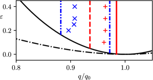
Figure 5: In a long system with $L_{x}=40\lambda_{0}$, the ESB (solid line) and the zigzag stability lines are shown for different boundary conditions in the $y$-direction and for two widths $L_{y}=2\lambda_{0},1.5\lambda_{0}$. Width $L_{y}=2\lambda_{0}$ (red): The vertical solid line marks the zigzag stability boundary $q_{zz}$ for BCI, the vertical dashed line $q_{zz}$ for PBC and the $+$-symbols mark $q_{zz}$ for BCII. Width $L_{x}=1.5\lambda_{0}$ (blue): The vertical dash-dotted line gives $q_{zz}$ for BCI, dash-dot-dotted line for PBC and the crosses $\times$ mark $q_{zz}$ for BCII.

In Fig. 5 the zigzag boundary crosses for different boundary conditions the Eckhaus-boundary (solid curve) at different values of $\varepsilon$. For control parameter values below this intersections of the zigzag and the Eckhaus boundary the systems behaves quasi-one dimensional. I.e. below these $\varepsilon$ the zigzag (ZZ) instability becomes irrelevant, because the Eckhaus instability sets in earlier.

Since the ESB depends for small system lengths $L_{x}$ on the boundary condition in the $x$-direction, the crossing of the ZZ and the Eckhaus stability boundary depends on the boundary conditions in the $x$ and $y$ direction. Therefore, the transition to a quasi one-dimensional behavior of stripe patterns depends on the control parameter $\varepsilon$, the system size and the used boundary condition in each direction. This is shown in Fig. 6 for $L_{x}=3\lambda_{0}$, where the first part of the curve label refers to the boundary condition in the $x$-direction and the second part refers to the boundary condition in the $y$-direction. Below these four curves in Fig. 6 the zigzag instability becomes irrelevant for these systems sizes and boundary conditions and the stripes behave one dimensional.

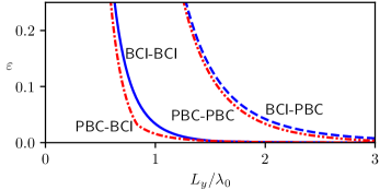
Figure 6: For a short system length $L_{x}=3\lambda_{0}$ and different combinations of BCI and PBC in the $x$- and the $y$-direction, the $\varepsilon$ position of the intersections between the ESB and the zigzag boundary is shown as function of the system width $L_{y}$. The first part of the curve designation describes the boundary in the $x$-direction.

Conversely, the zigzag instability limits above these curves in Fig. 6 the stability stripe pattern in the range $q<q_{0}$ for all the considered systems sizes and boundary conditions considered in this work, which is in contrast to Reference Yochelis:2020.1 .

V Examples of the nonlinear evolution of unstable stripes in finite systems

In this section, we exemplify how stripe patterns evolve after applying small perturbations from an unstable wavenumber $q<q_{0}$ through nothing but a zigzag instability to stripe patterns at a stable wavenumber. We use simulations of the SH model (1) in a rectangular domain with $L_{x}=40\lambda_{0}$ and $L_{y}=20\lambda_{0}$ and choose several different boundary conditions along the sides of the rectangle.

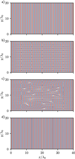
Figure 7: Shown are four snapshots of a simulation of the SH model in a rectangular domain of the side lengths $L_{x}=40\lambda_{0}$ and $L_{y}=20\lambda_{0}$; color scale represents the minimal (blue) and the maximal (red) values of $u$; no-flux boundary conditions (BCI) along the four boundaries and at $\varepsilon=0.4$. In (a) the initial solution with the wavenumber $q_{s}=0.9$ at time $t=0$ is shown, which is undulated by the zigzag instability in (b) at $t=10^{3}$. The resulting defects in (c) at $t=7.5\cdot 10^{3}$ heal rapidly due to the fixed phases at the edges and result in the solution with wavenumber $q=1.0$ at $t=66\cdot 10^{3}$ in (d).

Figure 8: Shown are four snapshots of a simulation of the SH model in a rectangle and the same parameters as in Fig. 7. Here, the no-flux boundary conditions are replaced by periodic boundary conditions (PBC) in the $x$-direction: starting from a solution with $q_{s}=0.9$ in (a) at time $t=0$, the solution becomes modulated at $t=2\cdot 10^{3}$ in (b). The defects appearing at $t=3.5\cdot 10^{3}$ in (c) are eliminated during further evolution and result in a solution with $q=1.0$ at $t=171\cdot 10^{3}$.

In Fig. 7 and Fig. 8 we started simulations in the rectangular domain by using a periodic initial pattern with $\varepsilon=0.4$ and a wavenumber $q=0.9$ which produce 36 stripes in the system. In Fig. 7 no-flux boundary conditions (BCI) are used along all four sides, whereas in Fig. 8 we replaced BCI by periodic boundary conditions in the $x$-direction. For the chosen system extensions the zigzag-stability boundaries is in both cases nearly indistinguishable at $q_{zz}\lesssim q_{0}$ as shown in Fig. 1, i.e. the starting wavenumber $q=0.9$ is far in the unstable range. While the two different boundary conditions leave the zigzag-stability boundary nearly untouched for larger $L_{y}=20\lambda_{0}$, the temporal evolution of the stripe patterns from an unstable to a stable wavenumber $q$ differs. Away from the boundaries at $x=0,L_{x}$ the unstable stripes with $q_{0}=0.9$ become according to the zigzag instability undulated, as can be seen in Fig. 7b) and Fig. 8b). For periodic boundary conditions at $x=0,L_{x}$ these stripe undulations occur also at the boundaries as shown in Fig. 8c). No-flux boundary conditions fix the phase of the stripe pattern with its maximum or minimum $u(x,y,t)$ at $x=0,L_{x}$. Therefore no undulations evolve at and near the boundaries, as indicated in Fig. 7c). According to the BCI induced constraint on the phase near the boundaries one has for BCI at $x=0,L_{x}$ a shorter transient time to reach finally a stable straight stripe pattern with $q_{0}\lesssim q$ as in indicated by Fig. 7d) and Fig. 8d). In both cases one ends up with a state composed of $40$ pattern units, i.e. with $q_{0}\lesssim q$. When we start simulations for both boundary conditions with an initial solution of wavenumber $q=0.975$, which corresponds to $39$ pattern units in the system, the pattern evolves again to a state of $40$ units with $q_{0}\lesssim q$.

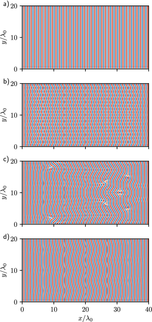
Figure 9: Shown are four snapshots of a simulation in a rectangle for the same parameters as in Fig. 7, but with type II boundary conditions (BCII) in the $y$-direction: a) Initial solution with wavenumber $q_{s}=0.9$ at $t=10$, b) $t=500$, c) $t=5.4\cdot 10^{3}$ and d) $t=109\cdot 10^{3}$ a stable solution with 39 periods and $q=0.975$.

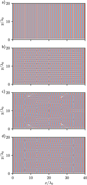
Figure 10: Shown are four snapshots of a simulation in a rectangle for the same parameters as in Fig. 7, but type III boundary conditions (BCIII) in the $y$-direction: a) Initial solution with wavenumber $q_{s}=0.9$ at $t=10$, b) $t=500$ and c) $t=5\cdot 10^{3}$ and in d) a solution with 38 stripes and $q=0.95$ so far.

In Fig. 9 and Fig. 10 we started simulations in a rectangular area with the same initial wavenumber $q=0.9$ and $\varepsilon$ as in Fig. 7. However, we replaced at $y=0,L_{y}$ no-flux boundary conditions (BCI) by the boundary conditions of type BCII in Fig. 9 and by type BCIII boundary condition in Fig. 10. As indicated in Fig. 5, the position of the zigzag-stability boundary $q_{zz}$ is in the case of BCII boundary conditions at $y=0,L_{y}$ stronger influenced in rather narrow systems than for no-flux boundary conditions, which is also true for BCIII boundary conditions.

However, the starting wavenumber $q_{s}=0.9$ is again considerably below $q_{zz}$ of PBC, which causes the strongest shift. One can recognize in Fig. 9 and Fig. 10 that the boundary conditions BCII and BCIII suppress stripe pattern close to $y=0,L_{y}$. Also for these boundary conditions at $y_{0}=0,L_{y}$ the unstable stripe pattern at $q_{s}=0.9$ becomes undulated in the bulk via the zigzag instability as indicated in Fig. 9b) and Fig. 10b). The further evolution is slightly different from the evolution shown in Fig. 7. The major difference is that at a similar simulations time the state in Fig. 9d) is composed of $39$ periodic units and in Fig. 10d) by $38$ periodic units.

VI Summary and conclusions

We investigated finite sizes effects on the multistability of supercritical bifurcating stripe patterns in rectangular domains using the generic Swift-Hohenberg model and the universal Newell-Whitehead-Segel equation. In two-dimensional extended isotropic systems, the wavenumber range of stable periodic patterns is limited by the longitudinal Eckhaus instability and the transverse zigzag instability. We show analytically and numerically for different combinations of boundary conditions along the edges of a rectangular domain that the range of wavenumbers for stable stripes increases with a reduction of the system size.

Note, also in finite systems the Eckhaus and zigzag instabilities remain the instabilities limiting the stable wavenumber range of stripe pattern for different boundary conditions. The zigzag instability remains the primary transversal instability also for no-flux boundary conditions in the longitudinal direction of stripe pattern. It is not replaced by another primary instability as recently claimed in Ref. Yochelis:2020.1 .

The enlargement of the stable wavenumber range of stripe patterns by the system size reduction is based on the following insights. The Eckhaus and zigzag instabilities are long-wavelength instabilities. By decreasing the system size, their destabilizing long-wavelength modes are increasingly suppressed. For periodic boundary conditions, an entire wavelength of a destabilizing mode must fit into the system, while for no-flux boundary conditions, for example, only half a wavelength of the destabilizing mode must fit into the finite system. That is, the smallest wavenumber $k$ of the perturbation is twice as large for periodic boundary conditions as for no-flux boundary conditions. According to our analytical results, the zigzag stability boundary is shifted proportionally to $k^{2}$. This means, for periodic boundary conditions in transverse direction, a reduction of the rectangle width shifts the stability boundary up to a factor of four more and increases the stable wavenumber range than for other boundary condition in transverse direction. The enlargement trend of the stable wavenumber range is similar for a reduction of the system length in longitudinal direction by shifting the Eckhaus boundary.

If boundary conditions that suppress the amplitude of the stripe pattern are taken in the transverse direction, the numerical results for the zigzag instability boundary lie between the analytical results for periodic and no-flux boundary conditions. This underlines the value of the presented analytical results also as an estimate for the location of the zigzag instability for other boundary conditions.

By reducing the system width sufficiently, the zigzag instability limit shifts to smaller values of the wave number than the lower Eckhaus stability limit for not to short systems. In this case, the zigzag instability is suppressed by the longitudinal instability that occurred previously. Below such system widths, the stripe pattern behaves quasi-one-dimensionally in two-dimensional systems. Again, the transition to quasi-one-dimensional behavior for periodic boundary conditions in the transverse direction occurs at already larger widths than for no-flux boundary conditions. Also for the transition to quasi-one-dimensional behavior, the analytical results for periodic and no-flux boundary conditions give a good estimate for the transition to quasi-one-dimensional behavior for other boundary conditions in transversal direction.

In the spatiotemporal evolution from a periodic stripe pattern with a wavenumber below the zigzag instability limit to a stripe pattern with a stable wavenumber, the influence of the boundary conditions is already noticeable for medium-sized systems with about 20 periodic stripes. This is shown for various combinations of boundary conditions along the rectangular domain in Section V. As these simulations show, in all cases the zigzag instability is the destabilizing mechanism, in contrast to the description in Ref. Yochelis:2020.1 .

The results of this work give also an estimate below which system lengths and widths, for given values of the control parameter, any emerging periodic pattern is also stable. These insights are important in investigations of e.g. Turing patterns in very small systems such as cells Sourjik:2017.1 . The here derived generic limitation of the stable wavenumber bands addresses also the so called robustness problem Maini:2012.1 ; Sourjik:2017.1 .

Data Availability

The data that support the findings of this study are available from the corresponding author upon reasonable request.

Appendix A Newell-White-Segel equation (NWSE) and stability of stripes

For completeness we include also the stability boundaries of stripes determined via the NWSE in Eq. (3) for no-flux boundary conditoins and periodic boundary conditions, which we can compare with the results of the SH model.

A.1 Linear stability of stripes within the NWSE

The NWSE has the stationary solutions

$$A=F_{n}e^{iQ_{n}x}$$ (26)

with the wavenumber $Q_{n}=q_{n}-q_{0}$ and the amplitude $F_{n}^{2}=(\varepsilon-\xi_{0}^{2}Q_{n}^{2})/g_{0}$. One has $F_{n}^{2}>0$ for $\varepsilon>\varepsilon_{0}$ and $F_{n}=0$ along the neutral curve:

$$\varepsilon_{0}={\xi_{0}^{2}}Q_{N}^{2}.$$ (27)

A.2 Zigzag instability within the NWSE

At first we investigate the zigzag instability of the stripe solution. For this we use the ansatz $A=(F+v(y))e^{iQ_{n}x}$ with a small $y$-dependent perturbation $v(y,t)$. By neglecting higher order terms of $v$ in Eq. (3), a linear equation for $v$ results:

$$\tau_{0}\partial_{t}v=\varepsilon v+\xi_{0}^{2}\left[iQ_{n}-\frac{i}{2q_{0}}\partial_{y}^{2}\right]^{2}v-g_{0}F^{2}v-F^{2}v^{*}.$$ (28)

This linear equation may be solved by

$$v=e^{\sigma t}\left[e^{iL_{j}y}v_{1}+e^{-iL_{j}y}v_{2}^{\ast}\right]\,,$$ (29)

where the wavenumber for no-flux boundary conditions at $y=0,L_{y}$ is $L_{j}=j\pi/L_{y}$ and for PBC $L_{j}=j2\pi/L_{y}$. Collecting the contributions $\propto e^{\pm iL_{j}y}$ gives two coupled homogeneous equations for $v_{1}$ and $v_{2}$ with the solubility condition

$$\begin{vmatrix}{\cal L}-\sigma\tau_{0}\qquad&-g_{0}F^{2}~{}~{}\\ -g_{0}F^{2}~{}~{}~{}&{\cal L}-\sigma\tau_{0}\end{vmatrix}=0$$ (30)

and the abbreviation

$${\cal L}=-\varepsilon-2\xi_{0}^{2}Q_{n}^{2}-\xi_{0}^{2}\left(Q_{n}+\frac{L_{j}^{2}}{2q_{0}}\right)^{2}\,.$$ (31)

Herein the growth rate of the perturbation is

$$\sigma\tau_{0}=-\frac{L_{j}^{2}}{2q_{0}}\left(2Q_{n}+\frac{L_{j}^{2}}{2q_{0}}\right)\,.$$ (32)

The stripe solution with the amplitude given by Eq. (26) is stable with respect to the perturbation in Eq. (29) in the range

$$Q_{n}>-\frac{L_{j}^{2}}{4q_{0}}\,=Q_{\text{zz}}.$$ (33)

A.3 Eckhaus-instability of stripes

Next we investigate the stability of stripe solutions with respect to longitudinal perturbations in long a quasi one-dimensional systems, i.e. with a small width $L_{y}=\pi/2q_{0}$.

In this case we investigate with Eq. (28) the dynamics of perturbations $v(x,t)$ with respect to the solution given by Eq. (26). We solve the linear equation (28) with the following ansatz

$$v=e^{\sigma t}\left(e^{iK_{l}x}v_{1}+e^{-iK_{l}x}v_{2}^{\ast}\right)\,,$$ (34)

and with the wavenumber $K_{l}=l\pi/L_{x}$. If the perturbation $v$ is growing with a wave number $K_{1}$, then during the instability process either nodes are added to the stripe solution, cf. Eq. (26), or removed. With the ansatz (34) in Eq. (28) and collecting the contributions $\propto e^{\pm iK_{j}x}$, gives two coupled homogeneous equations for $v_{1}$ and $v_{2}$ with the solubility condition

$$\begin{vmatrix}{\cal L}_{+}-\sigma\tau_{0}\qquad&-g_{0}F_{n}^{2}~{}~{}\\ -g_{0}F_{n}^{2}~{}~{}~{}&{\cal L}_{-}-\sigma\tau_{0}\end{vmatrix}=0$$ (35)

and

$${\cal L}_{\pm} =-\varepsilon+\underbrace{2\xi_{0}^{2}Q_{n}^{2}-\xi_{0}^{2}(Q_{n}^{2}\pm K_{l}^{2})}_{M_{\pm}}\,.$$ (36)

The growth rate of the perturbation expressed in terms of ${\cal L}_{\pm}$ is given by

$$\sigma =\frac{1}{2}\left({\cal L}_{+}+{\cal L}_{-}+\sqrt{({\cal L}_{+}-{\cal L}_{-})^{2}+4g_{0}^{2}F_{n}^{4}}\right)\,.$$ (37)

The neutral stability $\sigma=0$ condition for the $n$-node solution supplies

$${\cal L}_{+}{\cal L}_{-} =g_{0}^{2}F_{n}^{4}\,.$$ (38)

This gives the stability boundary $\varepsilon_{n}$ of the $n$-node solutions in the $\varepsilon_{n}-q_{n}$ plane

$$\varepsilon_{n}=\frac{M_{+}M_{-}-\xi_{0}^{4}Q_{n}^{4}}{M_{+}+M_{-}-2\xi_{0}^{2}Q_{n}^{2}}\,.$$ (39)

The $n$-node solution is stable (unstable) above (below) this curve.

A.4 Comparison of the NWSE to the SH model

As mentioned above the NWSE can derived from the SH model for the coefficients $\tau_{0}=1$, $\xi_{0}=2q_{0}$ and $g_{0}=3$ by a weakly nonlinear analysis CrossHo . This approximation holds near the threshold, where the neutral curve of the SH model Eq. (9) becomes also parabolic similar as in Eq. (27). For higher values of the control parameter $\varepsilon$, this two curves N for the SH and the NWSE differ as can be seen in Fig. 11. In contrast to this difference between the neutral curves of the NWSE (dashed lines) and the SH model (solid lines) the Eckhaus stability boundaries (E) is nearly identical. The zigzag instability (Z) even is indistinguishable for the two models.

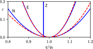
Figure 11: The neutral stability curves N, the Eckhaus-stability boundary E and the zigzag-stability boundary Z of stripes are shown as obtained for the Newell-White-Segel equation (solid lines) and the Swift-Hohenberg model (dashed lines). The zigzag-stability boundaries are indistinguishable (vertical solid line). System size $L_{x}=40\lambda_{0}$, $L_{y}=1.5\lambda_{0}$ and BCI in both directions.

Therefore the qualitative and quantitative results of this section, are with universal character since the universality of the amplitude equation.

References

- (1) M. C. Cross and P. C. Hohenberg. Pattern formation outside of equilibrium. Rev. Mod. Phys., 65:851, 1993.
- (2) P. Ball. The Self-Made Tapestry: Pattern Formation in Nature. Oxford Univ. Press, Oxford, 1998.
- (3) F. H. Busse. Nonlinear properties of convection. Rep. Prog. Phys., 41:1929, 1978.
- (4) A. Buka and L. Kramer. Pattern Formation in Liquid Crystals. Springer, Berlin, 1996.
- (5) I. Aranson and L. Kramer. The world of the complex Ginzburg–Landau equation. Rev. Mod. Phys., 74:99, 2002.
- (6) R. Kapral and K. Showalter, editors. Chemical Waves and Patterns. Springer, New York, 1995.
- (7) E. Bodenschatz, W. Pesch, and G. Ahlers. Recent Developments in Rayleigh-Bénard convection. Annu. Rev. Fluid Mech., 32:709, 2000.
- (8) A. S. Mikhailov and K. Showalter. Control of waves, patterns and turubulence in chemical systems. Phys. Rep., 425:79, 2006.
- (9) L. M. Pismen. Patterns and Interfaces in Dissipative Dynamics. Springer, Berlin, 2006.
- (10) S. Kondo and T. Miura. Reaction-diffusion model as a framework for unterstanding biological pattern formation. Science, 329:1616, 2010.
- (11) M. Lappa. Thermal Convection: Patterns, Evolution and Stability. Wiley, New York, 2009.
- (12) Y. Sasai. Cytosystems dynamics in self-organization of tissue architecture. Nature, 493:318, 2013.
- (13) E. Meron. Nonlinear Physics of Ecosystems. CRC Press, Boca Raton, FL, USA, 2015.
- (14) E. Meron. From pattern formation to function in living systems: Dryland Ecosystems as a case study. Annu. Rev. Condens. Matter Phys., 9:79, 2018.
- (15) M. Bär, R. Grossmann, S. Heidenreich, and F. Peruani. Self-Propelled Rods: Insights and Perspectives of Active Matter. Annu. Rev. Condens. Matter Phys., 11:441, 2020.
- (16) F. H. Busse. On the Stability of Two-Dimensional Convection in a Layer Heated from Below. J. Math & Phys., 46:140, 1967.
- (17) A. C. Newell, T. Passot, and J. Lega. Order parameter equations for patterns. Annu. Rev. Fluid Mech., 25:399, 1993.
- (18) A. C. Newell and J. A. Whitehead. Finite bandwidth finite amplitude convection. J. Fluid Mech., 38:279, 1969.
- (19) M. C. Cross, P. G. Daniels, P. C. Hohenberg, and E. D. Siggia. Phase-winding solutions in a finite container above the convective threshold. J. Fluid Mech., 55:155, 1983.
- (20) L. Kramer and P. C. Hohenberg. Effects of boundaries on periodic structures. Physica D, 13:352, 1984.
- (21) L. Kramer, E. Ben-Jacob, H. Brand, and M. C. Cross. Wavelength selection in systems far from equilibrium. Phys. Rev. Lett., 49:1891, 1982.
- (22) D. S. Cannell, M. A. Dominguez-Lerma, and G. Ahlers. Experiments on wave number selection in rotating Couette-Taylor flow. Phys. Rev. Lett., 50:1365, 1983.
- (23) M. C. Cross. Wave-number selection by soft boundaries near threshold. Phys. Rev. A, 29:391, 1984.
- (24) L. Kramer and W. Zimmermann. On the Eckhaus instability for spatially periodic patterns. Physica D, 16:221, 1985.
- (25) R. Heinrichs, G. Ahlers, and D. S. Cannell. Effects of Finite Geometry on the Wave Number in Taylor-Vortex Flow . Phys. Rev. Lett., 56:1794, 1986.
- (26) G. Ahlers, , D. S. Cannell, M. A. Dominguez-Lerma, and R. Heinrichs. Wavenumber-selection and Eckhaus in stability in Couette-Taylor flow. Physica D, 23D:202, 1986.
- (27) D. M. Raskin and P. A. J. de Boer. Rapid pole-to-pole oscillation of a protein required for directing division to the middle of Escherichia coli. Proc. Natl. Acad. Sci. USA, 96:4971, 1999.
- (28) F. Wu, B. G. C. van Schie, J. E. Keymer, and C. Dekker. Symmetry and scale orient Min protein patterns in shaped bacterial sculptures. Nat. Nanotechnol., 10:719, 2015.
- (29) S. M. Murray and V. Sourjik. Self-organization and positioning of bacterial protein clusters. Nat. Phys., 13:1006, 2017.
- (30) F. Bergmann, L. Rapp, and W. Zimmermann. Size matters for nonlinear (protein) wave patterns. New J. Phys. (FT), 20:072001, 2018.
- (31) A. D. Lander. Pattern, growth, and control. Cell, 144:955, 2011.
- (32) F. J. Thomsen, L. Rapp, F. Bergmann, and W. Zimmermann. Periodic patterns displace active phase separation. New J. Phys. (FT), 23:042002, 2021.
- (33) V. Eckhaus. Studies in Nonlinear Stability Theory. Springer, Berlin, 1965.
- (34) M. Boucif, J. E. Wesfreid, and E. Guyon. Role of boundary conditions on the mode selection in a buckling instability. J. Phys. Lett., 45:413, 1984.
- (35) H. Riecke and H. G. Paap. Stability and wave-vector restriction of axisymmetric Taylor vortex flow. Phys. Rev. A, 33:547, 1986.
- (36) M. Lowe and J. P. Gollub. Pattern selection near the onset of convection: The Eckhaus instability. Phys. Rev. Lett., 55:2575, 1985.
- (37) W. Zimmermann and L. Kramer. Wavenumber restriction in the buckling instability of a rectangluar plate. J. Phys. (Paris), 46:343, 1985.
- (38) M. A. Dominguez-Lerma, D. S. Cannell, and G. Ahlers. Eckhaus boundary and wave-number selection in rotating Couette-Taylor flow. Phys. Rev. A, 34:4956, 1986.
- (39) L. Kramer, H. Schober, and W. Zimmermann. Pattern competition and the decay of unstable patterns in quasi-one-dimensional systems. Physica D, 31:212, 1988.
- (40) L. S. Tuckermann and D. Barkley. Bifurcation analysis of the Eckhaus instability. Physica D, 46:57, 1990.
- (41) W. Pesch and L. Kramer. Nonlinear analysis of spatial structures in two–dimensional anisotropic pattern forming systems. Z. Physik B, 63:121, 1986.
- (42) E. Bodenschatz, W. Zimmermann, and L. Kramer. On electrically driven pattern-forming instabilities in planar nematics. J. Phys. (Paris), 49:1875, 1988.
- (43) M. C. Cross and H. Greenside. Pattern Formation and Dynamics in Nonequilibrium Systems. Cambridge Univ. Press, Cambridge, 2009.
- (44) H.S. Greenside and W. M. Coughran. Nonlinear pattern formation near the onset of Rayleigh-Bénard convection. Phys. Rev. A, 30:398, 1984.
- (45) M. Ruppert, F. Ziebert, and W. Zimmermann. Nonlinear patterns shaping their domain on which they live. New J. Phys. (FT), 22:052001, 2020.
- (46) A .P. Munuzuri, M. Dolnik, A. M. Zhabotinsky, and I. R. Epstein. Control of the Chlorine Dioxide-Iodine-Malonic Acid Oscillating Reaction by Illumination. J. Am. Chem. Soc., 121:8065, 1999.
- (47) M. Dolnik, I. Berenstein, A. M. Zhabotinsky, and I. R. Epstein. Spatial periodic forcing of turing structures. Phys. Rev. Lett., 87:238301, 2001.
- (48) R. Peter, M. Hilt, F. Ziebert, J. Bammert, J. Erlenkämper, N. Lorscheid, C. Weitenberg, A. Winter, M. Hammele, and W. Zimmermann. Stripe-hexagon competition in forced pattern-forming systems with broken up-down symmetry. Phys. Rev. E, 71:046212, 2005.
- (49) M. Hammele and W. Zimmermann. Harmonic versus subharmonic patterns in a spatially forced oscillating chemical reaction. Phys. Rev. E, 73:066211, 2006.
- (50) J. Schweizer, M. Loose, M. Bonny, K. Kruse, I. Mönch, and P. Schwille. Geometry sensing by self-organized protein patterns. Proc. Natl. Acad. Sci. USA, 109:15283, 2012.
- (51) L. Rapp, F. Bergmann, and W. Zimmermann. Pattern orientation in finite domains without boundaries. EL, 113:28006, 2016.
- (52) L. Kramer and H. Riecke. Wavelength selection in Rayleigh–Bénard convection. Z. Physik B, 59:245, 1985.
- (53) J. B. Swift and P. C. Hohenberg. Hydrodynamic fluctuations at the convective instability. Phys. Rev. A, 15:319, 1977.
- (54) L. A. Segel. Distant side-walls cause slow amplitude modulation of cellular convection. J. Fluid Mech., 38:203, 1969.
- (55) A. Z. Shapira, H. Uecker, and A. Yochelis. Stripes on finite domains: Why the zigzag instability is only a partial story. Chaos, 30:073104, 2020.
- (56) P. K. Maini, T. E. Wooley, R. E. Baker, E. A. Gaffney, and S. S. Lee. Turing’s model for biological pattern formation and the robustness problem. Interface Focus, 2:487, 2012.