A new first-order formulation of the Einstein equations exploiting analogies with electrodynamics

Abstract

When formulated as an initial boundary value problem, the Einstein and Maxwell equations are both systems of hyperbolic equations for which variables need to satisfy a set of elliptic constraints throughout evolution. However, while electrodynamics (EM) and magnetohydrodynamics (MHD) have benefited from a large number of evolution schemes that are able to enforce these constraints and are easily applicable to curvilinear coordinates, unstructured meshes, or $N$-body (or particle-in-cell) simulations, many of these techniques cannot be straightforwardly applied to existing formulations of the Einstein equations. With the aim of building a numerical scheme that exploits this existing technology, we develop a 3+1 a formulation of the Einstein equations which shows a striking formal resemblance to the equations of relativistic MHD and to EM in material media. The fundamental variables of this formulation are the frame fields, their exterior derivatives, and the Nester-Witten and Sparling forms. These mirror the roles of the electromagnetic 4-potential, the electromagnetic field strengths, the field excitations and the electric (in this case energy-momentum) current, respectively. It also possess the lapse function and shift vector as gauge freedoms, whose role corresponds exactly to that of the scalar part of the electromagnetic 4-potential. The formulation, that we name dGREM (for differential forms, general relativity and electromagnetism), is manifestly first order and flux-conservative, which makes it suitable for high-resolution shock capturing schemes and finite-element methods. Being derived using techniques from exterior calculus, it does not contain covariant but only exterior derivatives, which makes it directly applicable to any coordinate system and to unstructured meshes, and leads to a natural discretization in staggered grids potentially suitable for the use of well-known techniques for constraint preservation such as the Yee algorithm and constrained transport. Due to these properties, we expect this new formulation to be beneficial in simulations of many astrophysical systems, such as binary compact objects and core-collapse supernovae as well as cosmological simulations of the early universe. However we leave its numerical implementation for future work.

I Introduction

In the last few years the study of relativistic astrophysics and in particular of compact objects has made significant progress. The theoretical understanding of binary black holes, binary neutron stars and super-massive black holes has been validated by a string of impressive observations, such as the first detection of gravitational waves from BBHs(Abbott et al., 2016); the first and joint detection of GWs, a gamma ray burst (GRB) and a kilonova from a BNS system (Abbott et al., 2017a, b); and the first direct imaging of a super-massive accreting black hole (BH)(Event Horizon Telescope Collaboration et al., 2019, 2021).

These are systems exhibiting extreme complexity, and whose modeling requires the interplay of different areas of modern physics, such as relativistic gravitation, fluid dynamics, electrodynamics, nuclear physics, neutrino physics and many others. Therefore the theoretical study of these and other systems cannot be accomplished with purely analytical tools. NR has instead emerged as a powerful modeling tool.

The core approach of numerical relativity (NR) consists in finding approximate solutions to the partial differential equations describing the system at study, namely the Einstein’s field equations (EFE), by numerical integration. To this end, the equations of general relativity (GR) have first to be recast as an initial boundary value problem (IBVP). This can be accomplished in various ways. Examples include the generalized-harmonic formalism (Pretorius, 2005; Garfinkle, 2002; Lindblom et al., 2006); the characteristic-evolution formalism (Winicour, 2012); the conformal approach (Frauendiener and Friedrich, 2002; Hus, 2003) and fully-constrained formulations (Cordero-Carrión et al., 2008). These approaches however are not the subject of this work. Instead we operate in the context of the most commonly employed formalism, the so-called 3+1 formalism (Alcubierre, 2008; Rezzolla and Zanotti, 2013; Baumgarte and Shapiro, 2010).

In this formalism, the 4-dimensional spacetime of GR is foliated in a succession of purely spatial hypersurfaces; the EFE themselves split in 12 hyperbolic evolution equations, governing the evolution of the fields as time advances, and 4 elliptic constraint equations. The latter define constraints that the solution has to satisfy, and at the analytical level are always satisfied provided the initial data also satisfy them (and as such they must be solved to generate the initial data itself, see e.g. (Cook, 2000)). In order to obtain a true solution to the EFE, these constraints need to be satisfied. Violations may easily lead to unstable numerical simulations. While the constraints will be always satisfied at the analytical level, numerical truncation errors will easily cause violations that can accumulate and destabilize the evolution. It can even be shown that the ADM (Arnowitt et al., 1959; York, 1979) formulation of the EFE can be made strongly hyperbolic by assuming, among other conditions, that the momentum constraints are identically satisfied (Alcubierre, 2008). These considerations have motivated the search for alternative, more robust formulations of Einstein equations. Several approaches have been pursued to ensure stable numerical evolutions. A widely used and strongly hyperbolic formulation, namely BSSNOK, was introduced in Refs. (Shibata and Nakamura, 1995; Baumgarte and Shapiro, 1998; Brown, 2009; Beyer and Sarbach, 2004). In this formulation, the constraint violations cannot be dampened and will accumulate and grow over time. Despite this shortcoming, it allows for stable, long-term evolutions, yet in some particularly challenging test cases constraint violations can grow without bounds, typically crashing the evolution code (Alic et al., 2012; Brown et al., 2012).

A simple extension of the EFE to include propagating modes for the constraints, is to generalize a Lagrange multiplier approach, similar to the one adopted for electrodynamics (Dedner et al., 2002). The resulting family of formulations stemming from the Z4 formalism (Bona et al., 2003), most notably Z4c (Bernuzzi and Hilditch, 2010) and CCZ4 (Alic et al., 2012, 2013), include damping terms designed with the twofold aim of propagating the constraint violations away from where they occur and also damping them as they propagate (Gundlach et al., 2005).

It is important to understand that this approach does not guarantee exact fulfillment of the constraint equations. Techniques to control the growth of constraint violations however are commonly used in numerical electrodynamics. Maxwell’s equations include conditions such as the absence of magnetic monopoles, $\nabla\cdot\boldsymbol{B}=0$, which similarly to GR are elliptic equations that the solution of the corresponding evolution equations should satisfy at all times (Griffiths, 2017; Jackson, 1998). An example of a technique designed to handle these requirements is Dedner’s et al method (Dedner et al., 2002), employed successfully in numerical MHD and particle-in-cell (PIC) simulations.

Constraint damping was successfully applied in the first successful merger simulation (Pretorius, 2005), and it has been mainly adopted in simulations using the generalized-harmonic (GHG) formulation of the EFE (Pretorius, 2006; Lindblom et al., 2006). One important aspect of the GHG system is that the equations can trivially be recast in first-order form (Lindblom et al., 2006), which is more difficult for BSSNOK-like systems, such as FO-CCZ4 (Dumbser et al., 2018) or first-order BSSNOK (Brown et al., 2012). First-order formulations are particularly important when solving the EFE using finite elements or pseudospectral methods (Teukolsky, 2016), see Refs. (Dumbser et al., 2018), (Hébert et al., 2018) and (Bhattacharyya et al., 2021).

As recently pointed out, these first-order extensions are subject to additional curl-constraint, which can render the simulations unstable if not enforced. Generalizing the idea of divergence cleaning, Ref. (Dumbser et al., 2020) introduced the notion of curl cleaning, which requires to approximately solve four elliptic equations per constraint (using hyperbolic relaxation), and applied it to FO-CCZ4. This results in a system with a total of more than a hundred evolved variables, making the system very expensive to solve and implement efficiently.

Hence it would be beneficial to have a system of first-order equations that could be solved using simpler and cheaper approaches. In fact numerical electrodynamics has benefited also from another class of methods which are able to maintain a discretized version of the constraints satisfied to machine accuracy during the evolution, without adding additional equations to the system. The common feature of these methods is that the electromagnetic variables are not all defined and stored at the same spatial points in the computational domain, but on staggered grids. Belonging to this class of methods are the popular Yee algorithm (Yee, 1966) and constrained transport (CT) schemes (Evans and Hawley, 1988), widely used in numerical electrodynamics and MHD simulations.

A constraint preserving scheme for GR based on staggered grids was proposed by Ref. (Meier, 2003). This work identifies as crucial the role played by the second Bianchi identities in propagating the constraints, and develops a staggered finite-difference discretization that is able to satisfy them to machine precision in Riemann normal coordinates. However when such discretization is applied to general coordinates, the exact fulfillment of the identities is prevented by the non-cancellation of terms that are cubic in the Christoffel symbols, which appear as a result of the non-commutativity of covariant derivatives of the Riemann tensor. As a result the scheme’s ability to exactly propagation of constraints is bounded by the truncation error.

In the present work, we realize the importance of expressing equations as a system that relates differential forms with the tool of exterior calculus to obtain discretizations that fulfill the constraints to machine precision, and apply this idea to obtain a 3+1 formulation of GR. Being natural integrands over submanifolds, differential forms are very well suited to represent quantities such as total charges inside volumes or fluxes through surfaces. For this reason, integrating such equations yields a natural discretization that reflects the geometric properties of the equations themselves, and represents in a consistent way both the evolution and the constraint equations. Two important schemes derived from this idea are finite volume and constraint transport methods. In MHD, the former is able to achieve machine precision conservation of volume-integrated quantities (e.g. particle number density) by locating fluxes at the volume boundaries (cells faces), and the latter is able to achieve machine precision conservation of surface-integrated magnetic fluxes (which results in machine-precision fulfillment of $\nabla\cdot\boldsymbol{B}=0$) by locating electric fields at the surface boundaries (cells edges). I our endeavor we build upon the fact that a formulation of GR in the language of exterior calculus already exists (in fact it has already been proposed to exploit it in order to obtain coordinate invariant formulations suitable for numerical implementation (Frauendiener, 2006)).

The formulation we develop mirrors at the formal level the equations of covariant electrodynamics in a moving material medium (Jackson, 1998; Dumbser et al., 2017). We argue that this resemblance would allow to apply the knowledge and the methods developed in those disciplines to the evolution of dynamical spacetimes; in particular it would allow to develop CT schemes for NR, or to apply divergence- or curl-cleaning methods. In fact, it is conceivable that existing MHD solvers, e.g. (Etienne et al., 2015; Porth et al., 2016; Stone et al., 2020), could be adapted with minimal effort to solve the equations derived in this work to evolve dynamical spacetimes instead. This would hold even when adopting unstructured and moving meshes (Mocz et al., 2014).

This formulation, that we refer to as dGREM (for differential forms, general relativity and electromagnetism) also posses two other desirable features. Firstly, it contains only first order derivatives in both space and time, which can significantly simplify its discretization especially with some numerical schemes such as discontinuous Galerkin (dG) methods (Hesthaven and Warburton, 2008). Secondly, it can be written as a system of flux-balance laws, for the discretization of which a lot of expertise has been amassed over decades of work (Toro, 2009). To the best of the authors’ knowledge, no formulation of the Einstein equations available in the literature combines all of these advantages.

This work is organized as follows: after defining our notation (Sec. II), in Sec. III we introduce our exterior calculus-based techniques by applying them to the wave equation; Sec. IV revisits a formulation of GR as a system of equations written in terms of differential forms. Sec. V and Sec. VI are the central part of this work, in which we derive and present the proposed dGREM formulation. A summary of the results is given in Sec. VII, while several appendices provide details of derivations hinted at in the main text as well as a primer on the theory of exterior calculus.

II Notation and definitions

In this section we summarize the notation that is used in the rest of this work, since due to our reliance on concepts originating from the framework of exterior calculus, it may not be completely familiar to readers used to the NR literature. We direct the reader to Appendix A and references therein for more details on differential forms and exterior calculus. We also collect some definitions used throughout the article, mainly relating to the 3+1 split of GR.

We work within the usual spacetime of general relativity, i.e. a 4-dimensional, Lorentzian, at least twice differentiable manifold $\mathcal{M}$. We differentiate various type of indices on tensors and differential forms. Letters from the first half of the Latin alphabet ($a,b,c,\dots$) shall represent, in any basis, indices ranging from 0 to 3. In a coordinate basis, letters from the first half of the Greek alphabet ($\alpha,\beta,\gamma,\dots$) shall represent indices ranging from 0 to 3, and Latin letters from the second half of the alphabet ($i,j,k,\dots$) shall represent indices ranging from 1 to 3 (i.e. spatial components). The same convention will apply in a non-coordinate orthonormal basis, but using hatted characters, i.e. $\hat{\alpha},\hat{\beta},\hat{\gamma},\dots$ for indices from 0 to 3, and $\hat{i},\hat{j},\hat{k},\dots$ for indices from 1 to 3.

In what follows many objects contain non-tensorial indices. These objects are collections of differential forms, which we also call tensor-valued differential forms. The indices in these objects simply label the components in the collection and do not necessarily imply that the collection as a whole transform a tensor(see Sec. A for further details on tensor-valued differential forms and comments on the terminology). These indices will not be assigned any particular notation, although their non-tensorial nature will be indicated in the text.

Without referring to any particular basis, we indicate both tensors and differential forms with boldface characters; however in the abstract index notation that we preferentially employ, we drop the boldface font.

We define the following symbols: 
$\eta_{ab}$ Minkowski metric $\delta^{a}_{\ b}$ Kronecker delta $\epsilon_{abcd}$ Levi-Civita symbol $\varepsilon_{abcd}=\sqrt{-g}\epsilon_{abcd}$ volume form $\varepsilon^{abcd}$ Levi-Civita tensor (dual of volume form) $\boldsymbol{e}_{a}$ vector basis $\boldsymbol{\theta}^{a}$ dual basis $\partial$ partial derivative $\nabla$ covariant derivative $\boldsymbol{d}$ exterior derivative $\boldsymbol{D}$ covariant exterior derivative $\mathcal{L}$ Lie derivative $\star$ Hodge dual  
 
where $g$ denotes the determinant of the metric (see below). Note that all definitions above, even when written with coordinate basis indices, are valid in the case of non-coordinate bases too; and that in the definition of basis vectors and forms, the indices are non-tensorial, simply labeling objects in a collection.

While the objects we work with are denoted as scalars, vectors, tensors and differential forms, we actually always mean scalar fields, vector fields, tensor fields and fields of differential forms respectively, even when this is not explicitly stated. The same holds for objects that are not tensorial in nature, such as connection coefficients.

The manifold $\mathcal{M}$ is provided with a metric tensor $g_{\mu\nu}$, for which we choose the “mostly plus” signature $(-,+,+,+)$, and whose determinant is denoted by $g$. We also summarize here the framework of the 3+1 split of GR, which we employ in order to recast the Einstein equations as an initial value problem (see standard NR textbooks such as (Alcubierre, 2008; Rezzolla and Zanotti, 2013; Baumgarte and Shapiro, 2010) for more details). We assume that the spacetime can be foliated in a sequence of tridimensional, purely spatial hypersurfaces $\Sigma_{t}$ (i.e. the spacetime is assumed to be hyperbolic), each of which is parametrized by a value of a function $t$. We define the future-directed unit normal $n_{\mu}=-\alpha\nabla_{\mu}t$, where the lapse function $\alpha$ equals $\alpha=-1/g^{tt}$. From $n_{\mu}$ we can construct the metric restricted to each hypersurface $\gamma_{\mu\nu}=g_{\mu\nu}+n_{\mu}n_{\nu}$, which is purely spatial. Considering now the vector $t^{\mu}=g^{\mu\nu}\nabla_{\nu}t$, we identify it with our basis’ temporal vector (i.e. we choose a basis adapted to the foliation) and decompose it in a part parallel to $n^{\mu}$ and one perpendicular to it: $t^{\mu}=\boldsymbol{e}_{t}=\partial_{t}=\alpha n^{\mu}+\beta^{\mu}$. The purely spatial vector $\beta^{\mu}$ is called the shift vector. With these definitions in place we can then state the expressions of $n_{\mu}$ and $g_{\mu\nu}$ (or the line element $\textnormal{d}s$) in a coordinate basis:

$$n_{\mu}=(-\alpha,0,0,0)\quad\textnormal{and}\quad n^{\mu}=\frac{1}{\alpha}(1,-\beta^{i})^{T}$$

$$\textnormal{d}s=-(\alpha^{2}+\beta_{i}\beta^{i})\textnormal{d}t^{2}+2\beta_{i}\textnormal{d}t\textnormal{d}x^{i}+\gamma_{ij}\textnormal{d}x^{i}\textnormal{d}x^{j}\,,$$

where we have denoted with $x^{i}$ the spatial coordinates in any hypersurface $\Sigma_{t}$ and the ^T superscript indicates matrix transposition. We indicate with $\gamma$ the determinant of $\gamma_{ij}$, $\gamma=\det(\gamma_{ij})$, and note that $\sqrt{g}=\alpha\sqrt{\gamma}$.

Finally, we define the purely spatial extrinsic curvature $K_{ij}=-\frac{1}{2}\mathcal{L}_{\boldsymbol{n}}\gamma_{ij}$. As can be surmised from its definition, the extrinsic curvature is the rate of change of $\gamma_{ij}$ as measured by an observer moving along $n^{\mu}$, i.e. it is related to the time derivative of the three-metric $\gamma_{ij}$. We denote its trace by $K$.

III PDEs in the language of exterior calculus

Differential forms are natural integrands on submanifolds, and PDEs that can be written as relations between differential forms with the tools of exterior calculus can be naturally discretized by integration on appropriate volumes. When such a discretization is applied consistently, the resulting evolution scheme correctly reflects the geometric structure of the equations. In turn, this opens up the possibility of developing constraint-preserving evolution schemes.

In order to introduce the reader to our approach as outlined above, we apply it in this section to a well-known PDE. Namely, we explicitly formulate the standard wave equation on a generic spacetime in terms of differential forms. This helps us setting the stage for reformulating GR and the Einstein equations in the same language in the next section.

III.1 The wave equation

Rather than stating the usual wave equation (in terms of scalar or vector fields and ordinary derivatives) and showing how it can be expressed in terms of differential forms, we choose here to reverse the exposition order, i.e. stating the equation as a relation between differential forms and then recovering the usual formulation. This better reflects the derivation the dGREM formulation of GR in Sec. IV.

Consider a scalar field (or $0$-form) $\phi$, and its exterior derivative $\boldsymbol{J}=\boldsymbol{d}\phi$ which is of course a $1$-form. $\boldsymbol{J}$ satisfies the equation

$$-\star^{-1}\boldsymbol{d}\star\boldsymbol{J}=0\,.$$ (1)

Employing the components representation of the exterior derivative and of the Hodge dual, we can rewrite Eq. (1) as

$$\varepsilon^{\alpha\beta\gamma\nu}\,\partial_{[\nu}\left(\varepsilon_{\alpha\beta\gamma]\mu}\,J^{\mu}\right)=0\,.$$ (2)

Note that in this section we assume for simplicity a coordinate basis, hence the indices are labeled by Greek letters.

Recalling the definition of $\boldsymbol{\varepsilon}$ it is easy to see that the last equation becomes

$$\frac{1}{\sqrt{-g}}\partial_{\mu}\left(\sqrt{-g}\,J^{\mu}\right)=0\,,$$ (3)

expressing that the divergence of $\boldsymbol{J}$ must vanish. This was to be expected since operator in (1) (sometimes called the codifferential) is a generalization of the divergence operator (see Eq. (148)). Substituting the definition of $\boldsymbol{J}$ as the exterior derivative of $\phi$, this equation immediately implies

$$\frac{1}{\sqrt{-g}}\partial_{\mu}\left(\sqrt{-g}\,\partial^{\mu}\phi\right)=0\,,$$ (4)

i.e. the standard homogeneous wave equation for the field $\phi$ in a generic spacetime.

We now seek too express Eq. (4) via a 3+1 formulation, i.e. recasting it as an evolution equation for $\phi$. To this end let us define the following projections of $\boldsymbol{J}$:

$$\begin{split}\rho&=-n^{\mu}J_{\mu}\\ j_{i}&=\gamma^{\mu}_{\ i}J_{\mu}\,.\end{split}$$ (5)

Substituting these definitions in Eq. (3) and recalling the relationship between the unit normal $n^{\mu}$, the lapse $\alpha$ and the shift $\beta^{i}$, yields the equations

$$\begin{split}\partial_{t}\left(\sqrt{\gamma}\rho\right)+\partial_{i}\left(\sqrt{\gamma}\rho\mathcal{V}^{i}\right)&=0\,,\\ \partial_{t}j_{i}+\partial_{i}\left(\alpha\rho-\beta^{k}j_{k}\right)&=0\,,\end{split}$$ (6)

where $\mathcal{V}^{i}=\alpha j^{i}/\rho-\beta^{i}$ is the transport velocity of $\rho$.

These are evolution equations for (quantities related to) the components of $\boldsymbol{J}$. An evolution equation for $\phi$ itself can easily be recovered from the definition of $\rho$ and recalling that $J_{t}=\partial_{t}\phi$, resulting in

$$\partial_{t}\phi=\alpha\rho+\beta^{k}j_{k}\,.$$ (7)

The wave equation Eq. (4), or the system (6), is subject to a set of differential constraints. Working with differential forms, this can be seen as follows. The nilpotency of the exterior derivative, equation (129), immediately gives

$$\boldsymbol{d}\boldsymbol{J}=\boldsymbol{d}\boldsymbol{d}\phi=0\,.$$ (8)

This of course implies that $\star\boldsymbol{d}\boldsymbol{J}=0$, and by comparing with Eq. (149), we can expect this equation to be requiring the curl of $\boldsymbol{J}$ to vanish. Indeed switching to a components representation and using the variables $\rho$ and $j_{i}$, Eq. (8) is equivalent to:

$$\partial_{i}j_{k}-\partial_{k}j_{i}=0\,.$$ (9)

These are 3 constraint equations for the spatial components of $\boldsymbol{J}$ (a fourth equation, stemming from considering the time components and involving the variable $\rho$, turns out to be identical to the evolution equation for $j_{i}$).

Eqs. (9) simply assert the commutativity of second spatial derivatives of $\phi$, but as the wave equation itself they can be stated much more compactly and expressively in terms of differential forms.

As mentioned in the introduction, writing the system in terms of differential forms can be also useful to determine the spatial localization of variables for a constraint preserving discretization. However, the direct integration of equations (1) and (8), would yield a four dimensional discretization staggered in time. For methods such as finite-volume, it is more convenient to derive a semi-discrete evolution equation with all variables located on the hypersurface $\Sigma_{t}$. In order to achieve this, we employ Cartan’s “magic” formula (see Eq. (130) in Appendix A), and compute the Lie derivative of $\boldsymbol{J}$ and $\star\boldsymbol{J}$, with respect to the basis vector $\boldsymbol{e}_{t}$, which coincides with $\partial_{t}$.

$$\begin{split}\mathcal{L}_{\boldsymbol{e}_{t}}\boldsymbol{J}&=\boldsymbol{d}(\boldsymbol{e}_{t}\cdot\boldsymbol{J})\,,\\ \mathcal{L}_{\boldsymbol{e}_{t}}\star\boldsymbol{J}&=\boldsymbol{d}(\boldsymbol{e}_{t}\cdot\star\boldsymbol{J})\,,\end{split}$$ (10)

or

$$\partial_{t}\boldsymbol{J} =\boldsymbol{d}(\alpha\rho+\beta^{k}j_{k})\,,$$ (11)

$$\partial_{t}\star\boldsymbol{J} =\boldsymbol{d}\boldsymbol{F}\,,$$ (12)

where the flux form $\boldsymbol{F}$ is defined as

$$\boldsymbol{F}=\varepsilon_{ijk}(\alpha j^{i}-\beta^{i})\left(\frac{1}{2}\boldsymbol{d}x^{j}\wedge\boldsymbol{d}x^{k}\right)\,.$$

The nontrivial components of (11) and (12) give identical equations to those in (6); however, the advantage of writing them in this way is that the submanifolds on which they should be integrated become explicit. All terms in (11) are 1-forms, and all terms in (12) are 3-forms, which invites to integrate them, respectively, on curves and volumes. For the purpose of a numerical scheme which decomposes a three-dimentional simulation domain in zones, this corresponds to integrate the equations over zone edges and zone volumes. After applying the Stokes theorem (146), exterior derivatives are replaced by evaluations of the forms on zone boundaries (i.e. respectively, on zone vertices and zone faces).

It is straightforward to see that such discretization conserves globally the volume-integrated ‘charge’ $\rho$: since faces are shared by two zones, the amount of flux leaving one zone and entering the other will contribute with opposite signs to the time update of each zone’s content, and the total charge content in the simulation domain will remain constant to machine precision as long as there is no flux through the simulation boundaries.

The discretization also fulfills constraint a discretized version of equation (9) to machine precision. This can be seen by integrating equation (8) over a zone face (i.e. a surface, since it is a 2-form). The application of Stoke’s theorem once more transforms the exterior derivative into the sum of the forms $\boldsymbol{J}$ integrated on the contour formed by the edges surrounding that face (i.e. the circulation around it). Also in this case, each of the scalars $\alpha\rho+\beta^{k}j_{k}$ defined at zone vertices will be shared by two edges and contribute to their time update of $\boldsymbol{J}$ with opposite signs, canceling their contributions to the circulation. The discretization is therefore able to preserve an integrated version of constraint (9) to machine precision when supplied with constraint-fulfilling initial data.

IV General relativity in the language of exterior calculus

In this section, we first lay the groundwork to derive the dGREM formulation by outlining a reformulation of the Einstein equations in terms of exterior calculus and using objects known as the Nester-Witten and Sparling forms. This results in writing the Sparling equation, which is fully equivalent to the EFE.

We then introduce a change of variables and a particular choice of connection which ultimately allows us to re-express the Sparling equation, and therefore the EFE, as a system of evolution equations resembling the Maxwell equation of electrodynamics, i.e. the titular dGREM formulation.

Let’s define for convenience the “hypersurface forms” as (Szabados, 1992):

$$\boldsymbol{\Sigma}_{a_{1}\dots a_{r}}=\frac{1}{(4-r)!}\varepsilon_{a_{1}\dots a_{r}a_{r+1}\dots a_{4}}\boldsymbol{\theta}^{a_{r+1}}\wedge\dots\wedge\boldsymbol{\theta}^{a_{4}}\,.$$ (13)

Loosely speaking, they can be thought as (the dual forms to) vectors orthogonal to submanifolds spanned by given subsets of the basis $\boldsymbol{\theta}^{a_{1}}\wedge\dots\wedge\boldsymbol{\theta}^{a_{4}}$, e.g. the $3$-form $\Sigma_{0}=\varepsilon_{0123}\boldsymbol{\theta}^{1}\wedge\boldsymbol{\theta}^{2}\wedge\boldsymbol{\theta}^{3}$ is orthogonal to the tridimensional hypersurface spanned by $\boldsymbol{\theta}^{1}$, $\boldsymbol{\theta}^{2}$ and $\boldsymbol{\theta}^{3}$. They satisfy the identity

$$\boldsymbol{\theta}^{b}\wedge\boldsymbol{\Sigma}_{a_{1}\dots a_{r}}=(-1)^{r+1}r\delta^{b}_{\ [a_{1}}\boldsymbol{\Sigma}_{a_{2}\dots a_{r}]}\,.$$ (14)

For a manifold with curvature and torsion described, respectively, by the 2-forms $\boldsymbol{\Omega}^{a}_{\ b}$ and $\boldsymbol{\Xi}^{a}$, the connection forms $\boldsymbol{\omega}^{a}_{\ b}$ (see App. A for a definition) are completely specified by Cartan’s structure equations,

$$\boldsymbol{\Xi}^{a} =\boldsymbol{d}\boldsymbol{\theta}^{a}+\boldsymbol{\omega}^{a}_{\ b}\wedge\boldsymbol{\theta}^{b}$$ (15)

$$\boldsymbol{\Omega}^{a}_{\ b} =\boldsymbol{d}\boldsymbol{\omega}^{a}_{\ b}+\boldsymbol{\omega}^{a}_{\ c}\wedge\boldsymbol{\omega}^{c}_{\ b}\,,$$ (16)

and by the condition of metric compatibility of the connection,

$$\boldsymbol{d}g_{ab}=\boldsymbol{\omega}_{ab}+\boldsymbol{\omega}_{ba}\,.$$ (17)

Note that in this last equation the individual components of the metric are seen as $0$-forms, i.e. the metric itself is a tensor-valued $0$-form, hence it is possible to apply the exterior derivative to it.

The curvature and torsion forms are related to the Riemann and the torsion tensors $R^{a}_{\ bcd}$ and $T^{a}_{\ bc}$ by

$$\boldsymbol{\Omega}^{a}_{\ b}\wedge\boldsymbol{\Sigma}_{cd} =R^{a}_{\ bcd}\;\boldsymbol{\Sigma}$$ (18)

$$\boldsymbol{\Xi}^{a} =T^{a}_{\ bc}\;\boldsymbol{\theta}^{b}\wedge\boldsymbol{\theta}^{c}\,.$$ (19)

It can be shown (Szabados, 1992; Frauendiener, 2006) that the curvature form is related to the Ricci tensor $R^{b}_{\ c}$, the curvature scalar $R=R^{b}_{\ b}$ and the Einstein tensor $G^{c}_{\ d}=R^{c}_{\ d}-Rg^{c}_{\ d}$ in the following ways:

$$\boldsymbol{\Omega}^{ab}\wedge\boldsymbol{\Sigma}_{ac} =R^{b}_{\ c}\;\boldsymbol{\Sigma}$$ (20)

$$\boldsymbol{\Omega}^{ab}\wedge\boldsymbol{\Sigma}_{ab} =R\;\boldsymbol{\Sigma}$$ (21)

$$-\frac{1}{2}\boldsymbol{\Omega}^{ab}\wedge\boldsymbol{\Sigma}_{dab} =G^{c}_{\ d}\;\boldsymbol{\Sigma}_{c}\,.$$ (22)

By taking the exterior derivative of Cartan’s structure equations (Eqs. 15–16), it is possible to obtain the first and second Bianchi identities,

$$\boldsymbol{d}\boldsymbol{\Xi}^{a} =\boldsymbol{\Omega}^{a}_{\ e}\wedge\boldsymbol{\theta}^{e}-\boldsymbol{\omega}^{a}_{\ e}\wedge\boldsymbol{\Xi}^{e}$$ (23)

$$\boldsymbol{d}\boldsymbol{\Omega}^{a}_{\ b} =\boldsymbol{\Omega}^{a}_{\ e}\wedge\boldsymbol{\omega}^{e}_{\ b}-\boldsymbol{\omega}^{a}_{\ e}\wedge\boldsymbol{\Omega}^{e}_{\ b}\,,$$ (24)

which for a manifold with no torsion and in a coordinate basis take the usual form

$$R_{\mu\alpha\beta\gamma}+R_{\mu\beta\gamma\alpha}+R_{\mu\gamma\alpha\beta} =0\,,$$ (25)

$$\nabla_{\alpha}R_{\mu\nu\beta\gamma}+\nabla_{\beta}R_{\mu\nu\gamma\alpha}+\nabla_{\gamma}R_{\mu\nu\alpha\beta} =0\,.$$ (26)

To formulate general relativity as a system with exterior derivatives, we first define a 2-form $\boldsymbol{u}_{a}$, known as the Nester-Witten form (Szabados, 1992; Frauendiener, 1990, 2006):

$$\boldsymbol{u}_{a}\coloneqq-\frac{1}{2}\boldsymbol{\omega}^{bc}\wedge\boldsymbol{\Sigma}_{abc}\,.$$ (27)

Taking its exterior derivative and using the two Cartan structure equations, we obtain

$$\begin{split}\boldsymbol{d}\boldsymbol{u}_{a}=&-\frac{1}{2}\boldsymbol{\Omega}^{bc}\wedge\boldsymbol{\Sigma}_{abc}+\frac{1}{2}\boldsymbol{\Xi}^{d}\wedge\boldsymbol{\omega}^{bc}\wedge\boldsymbol{\Sigma}_{abcd}\\ &-\frac{1}{2}\left(\boldsymbol{\omega}^{b}_{\ d}\wedge\boldsymbol{\omega}^{dc}\wedge\boldsymbol{\Sigma}_{abc}+\boldsymbol{\omega}^{d}_{\ a}\wedge\boldsymbol{\omega}^{bc}\wedge\boldsymbol{\Sigma}_{dbc}\right)\,.\end{split}$$ (28)

The terms in parenthesis can be grouped in a 3-form known as the Sparling form:

$$\boldsymbol{t}_{a}\coloneqq-\frac{1}{2}\left(\boldsymbol{\omega}^{b}_{\ d}\wedge\boldsymbol{\omega}^{dc}\wedge\boldsymbol{\Sigma}_{abc}+\boldsymbol{\omega}^{d}_{\ a}\wedge\boldsymbol{\omega}^{bc}\wedge\boldsymbol{\Sigma}_{dbc}\right)\,,$$ (29)

whose pull-backs in different basis are related to different expressions for the gravitational energy-momentum. In particular, in a coordinate basis it is the Einstein pseudotensor (Frauendiener, 1990). For convenience, let us define $t^{b}_{\ a}$ such that

$$\boldsymbol{t}_{a}=t^{b}_{\ a}\boldsymbol{\Sigma}_{b}\,.$$ (30)

Assuming no torsion, relation (22) and equation (28) can be used to obtain the Sparling equation:

$$\boldsymbol{d}\boldsymbol{u}_{a}=\boldsymbol{t}_{a}+\kappa\boldsymbol{T}_{a}\,,$$ (31)

where the non-gravitational energy-momentum 3-form $\boldsymbol{T}_{a}$ is defined as

$$\boldsymbol{T}_{a}=T^{\mu}_{\ a}\boldsymbol{\Sigma}_{\mu}\,,$$ (32)

and where $T^{\mu}_{\ a}$ are the components of the energy-momentum tensor.

At this point a few comments are necessary. First of all, Eq. (31) is equivalent to the Einstein equations (Szabados, 1992; Frauendiener, 1990, 2006), and the sum of the Nester-Witten and Sparling forms is related to the Einstein tensor by

$$\boldsymbol{d}\boldsymbol{u}_{a}-\boldsymbol{t}_{a}=G^{b}_{\ a}\boldsymbol{\Sigma}_{b}\,,$$ (33)

or in components form,

$$G^{c}_{\ a}=\frac{1}{\sqrt{-g}}\partial_{b}\left[\sqrt{-g}\,(-\star\boldsymbol{u}_{a})^{\ bc}\right]-t^{c}_{\ a}\,.$$ (34)

This equivalence holds despite the fact that the index in the objects $\boldsymbol{u}_{a}$ and $\boldsymbol{t}_{a}$ is non-tensorial, i.e. the components of the Nester-Witten form $u_{abc}=(\boldsymbol{u}_{a})_{bc}$ are not part of a single 3-indices tensor, but belong to a collection of four 2-forms labeled by the index $a$, which transform as ${0\choose 2}$-tensors with indices $b$ and $c$ (see also Appendix A).

This also means that the objects $\boldsymbol{u}_{a}$ and $\boldsymbol{t}_{a}$ are not unique: a different choice of basis 1-forms from which to compute the connection will lead to different collections of objects, although Eq. (31) will still hold, in the same way as the choice of different basis and connections does not alter the validity of the Einstein equations.

Although the non-tensorial behavior of these quantities might be startling, this behavior is natural, as it is linked to the local flatness of space-time. In the language of tensors, various quantities (such as the metric first partial derivatives or energy-momentum pseudotensors) can be made to vanish locally in a free-falling frame. This is possible owing to the non-tensorial nature of these objects, as tensors cannot made to vanish by a coordinate (i.e. linear) transformation. By the same token e.g. the Sparling form, which is related to various kinds of energy-momentum pseudotensors (Szabados, 1992; Frauendiener, 1990), displays a similar behavior thanks to its own non-tensorial nature.

V Exploiting the analogies with Maxwell’s equations

V.1 Evolution equations and constraints

Equation (31) presents the Einstein equations as a set of four equations with a structure very similar to that of the inhomogeneous Maxwell equations, i.e. with the exterior derivative of a 2-form at the left-hand side and a conserved current at the right-hand side. In fact, taking the exterior derivative of equation (31) it can be seen that the four currents $\boldsymbol{J}_{a}=\star(\boldsymbol{t}_{a}+\kappa\boldsymbol{T}_{a})$ are globally conserved. Each antisymmetric tensor $u_{a\mu\nu}$ in the Nester-Witten form plays the role of the Maxwell 2-form, and in a coordinate basis, equation (31) takes a form completely analogous to that of the inhomogeneous Maxwell equations,

$$\partial_{b}\sqrt{-g}\,(-\star u_{a}^{\ \ bc})=\sqrt{-g}(t^{c}_{\ a}+\kappa T^{c}_{\ a})\,.$$ (35)

Comparing (35) with (34), its equivalence to the Einstein equations becomes clear.

Exploiting further the similarity with electrodynamics, we can define the following projections of the Nester-Witten form and its dual

$$H_{a}^{\ \mu}\coloneqq u_{a}^{\ \mu\nu}n_{\nu}\qquad\text{and}\qquad D_{a}^{\ \mu}\coloneqq-\star u_{a}^{\ \mu\nu}n_{\nu}\,.$$ (36)

This allows to decompose these forms as

$$u_{a\mu\nu} =n_{\mu}H_{a\nu}-n_{\nu}H_{a\mu}+\varepsilon_{\mu\nu\alpha\beta}n^{\alpha}D_{a}^{\ \beta}\,,$$ (37)

$$\star u_{a\mu\nu} =-n_{\mu}D_{a\nu}+n_{\nu}D_{a\mu}+\varepsilon_{\mu\nu\alpha\beta}n^{\alpha}H_{a}^{\ \beta}\,.$$ (38)

Defining as well the following projections of the components of the Sparling form and the energy-momentum tensor ,

$$\begin{split}\rho_{a}&\coloneqq n_{\mu}t^{\mu}_{\ a}\,,\\[1.42262pt] s^{i}_{\ a}&\coloneqq\gamma^{i}_{\ \mu}t^{\mu}_{\ a}\,,\\[1.42262pt] P_{a}&\coloneqq n_{\mu}T^{\mu}_{\ a}\,,\\[1.42262pt] S^{i}_{\ a}&\coloneqq\gamma^{i}_{\ \mu}T^{\mu}_{\ a}\,.\end{split}$$ (39)

Eqs. (35) can be separated into four constraint equations

$$\mathcal{C}_{a}\coloneqq\partial_{i}\sqrt{\gamma}D_{a}^{\ i}-\sqrt{\gamma}(\rho_{a}+\kappa P_{a})=0\,,$$ (40)

and twelve evolution equations

$$\begin{split}&\mathcal{F}^{k}_{\ a}\coloneqq\\ &\partial_{t}\sqrt{\gamma}D_{a}^{\ k}-\partial_{i}\sqrt{\gamma}(\alpha\varepsilon^{kij}H_{aj}+\beta^{i}D_{a}^{\ k}-\beta^{k}D_{a}^{\ i})\\ &+\sqrt{\gamma}(j^{k}_{\ a}+\kappa J^{k}_{\ a})=0\end{split}$$ (41)

where

$$j^{k}_{\ a}= \alpha s^{k}_{\ a}-\beta^{k}\rho_{a},$$ (42)

$$J^{k}_{\ a}= \alpha S^{k}_{\ a}-\beta^{k}P_{a}\,.$$ (43)

The fulfillment of equations (40) is equivalent to that of the Einstein constraints. This can be seen by the definition of the usual Hamiltonian and momentum constraints and the 3+1 evolution equations (Frittelli, 1997) as

$$\begin{split}\mathcal{H}&\coloneqq n^{\mu}n^{\nu}(G_{\mu\nu}-\kappa T_{\mu\nu})=0\,,\\ \mathcal{M}_{i}&\coloneqq\gamma^{\mu}_{\ i}n^{\nu}(G_{\mu\nu}-\kappa T_{\mu\nu})=0\,,\\ \mathcal{E}_{ij}&\coloneqq\gamma^{\mu}_{\ i}\gamma^{\nu}_{\ j}(G_{\mu\nu}-\kappa T_{\mu\nu})=0\,,\end{split}$$ (44)

from which

$$\begin{split}\mathcal{C}_{0}&=-\mathcal{H}\,,\\ \mathcal{C}_{i}&=-\mathcal{M}_{i}/\alpha\,,\\ \mathcal{F}^{i}_{\ 0}&=\alpha\mathcal{M}^{i}+\beta^{i}\mathcal{H}\,,\\ \mathcal{F}^{i}_{\ j}&=\mathcal{E}^{i}_{\ j}+\beta^{i}\mathcal{M}_{j}/\alpha\,,\end{split}$$ (45)

and therefore $\mathcal{C}_{a}=0$ is equivalent to $\mathcal{M}_{i}=0$ and $\mathcal{H}=0$. The twice-contracted second Bianchi identities imply that if the Hamiltonian constraint is fulfilled on a space-like hypersurface, its fulfillment on the “next” hypersurface is guaranteed as long as the momentum constraints are satisfied exactly and the system is evolved using evolution 3+1 Einstein equations (Frittelli, 1997). Similar equations for the propagation of constraints $\mathcal{C}_{a}$ can be obtained after taking the exterior derivative of the Sparling equation (31). This results in a set of equations equivalent to the twice-contracted second Bianchi identities, of the form

$$\partial_{t}\sqrt{-g}\mathcal{C}_{a}+\partial_{i}\sqrt{-g}\mathcal{F}^{i}_{\ a}=0\,.$$ (46)

Therefore, also in this case the evolution equations for $D_{k}^{\ i}$ and the exact fulfillment of the momentum constraints $\mathcal{C}_{i}$ are sufficient to propagate the fulfillment of $\mathcal{C}_{0}$ between subsequent hypersurfaces.

V.2 Energy-momentum conservation

The exterior derivative of equation (31) can also be used to obtain evolution equations for the “charge densities” $\rho_{a}$ and $P_{a}$, as it expresses the global conservation of the sum of their currents,

$$\boldsymbol{d}(\boldsymbol{t}_{a}+\kappa\boldsymbol{T}_{a})=0\,.$$ (47)

Together with the local conservation of matter energy-momentum $\boldsymbol{D}\boldsymbol{T}_{a}=0$, this gives

$$\boldsymbol{d}\boldsymbol{T}_{a} =\boldsymbol{\omega}^{b}_{\ a}\wedge\boldsymbol{T}_{b}\qquad\text{and}$$ (48)

$$\boldsymbol{d}\boldsymbol{t}_{a} =-\kappa\ \boldsymbol{\omega}^{b}_{\ a}\wedge\boldsymbol{T}_{b}\,,$$ (49)

or in component form and in a coordinate basis,

$$\partial_{\mu}\sqrt{-g}\ T^{\mu}_{\ a} =\sqrt{-g}\ \omega^{b}_{\ a\mu}T^{\mu}_{\ b}\qquad\text{and}$$ (50)

$$\partial_{\mu}\sqrt{-g}\ t^{\mu}_{\ a} =-\kappa\ \sqrt{-g}\ \omega^{b}_{\ a\mu}T^{\mu}_{\ b}\,.$$ (51)

Substituting the projections defined above (Eq. 39),

$$\partial_{t}\sqrt{\gamma}\rho_{a}+\partial_{i}\sqrt{\gamma}(\alpha s^{i}_{\ a}-\beta^{i}\rho_{a}) =-\kappa\sqrt{\gamma}Q_{a}\,,$$ (52)

$$\partial_{t}\sqrt{\gamma}P_{a}+\partial_{i}\sqrt{\gamma}(\alpha S^{i}_{\ a}-\beta^{i}P_{a}) =\ \sqrt{\gamma}Q_{a}\,,$$ (53)

where

$$Q_{a}=-(\omega^{b}_{\ at}+\omega^{b}_{\ ai}\beta^{i})P_{b}+\alpha\omega^{b}_{\ ai}S^{i}_{\ b}\,.$$ (54)

The physical interpretation of Eqs. (31), (48) and (49) can be that of four vector fields described by the four 2-forms $\boldsymbol{u}_{a}$ which have as sources two currents $\star\kappa\boldsymbol{T}_{a}$ and $\star\boldsymbol{t}_{a}$. The sum of the latter two is globally conserved, but they exchange charge (in this case, energy and momentum) via the “force” term $\kappa\boldsymbol{\omega}^{b}_{\ a}\wedge\boldsymbol{T}_{b}$. These currents are those of gravitational ($\star\boldsymbol{t}_{a}$) and non-gravitational ($\star\kappa\boldsymbol{T}_{a}$) energy and momentum. Eqs. (40) and (41) are the analogue of the inhomogeneous Maxwell equations in 3+1 form, and equations (52) and (53) that of the conservation of the two charges.

While Eqs. (52) and (53) convey an interesting physical picture of energy exchange between the purely gravitational and the matter sector, there is another possibility of how to read these equations in practice. Adding up (52) and (53), we obtain

$$\partial_{t}\left[\sqrt{\gamma}\left(\rho_{a}+\kappa P_{a}\right)\right]$$

$$+ \partial_{i}\left[\sqrt{\gamma}\left(\alpha\left(s^{i}_{\ a}+\kappa S^{i}_{\ a}\right)-\beta^{i}\left(\rho_{a}+\kappa P_{a}\right)\right)\right]=0\,.$$ (55)

When comparing this equation with the equation of energy-momentum conservation (50), it is striking to see that using the Sparling form all source terms in (V.2) have disappeared. In this formulation, the geometric source terms of Eq. (50) have been recast into a fully flux conservative form. A similar observation has recently also been made by Clough (2021). While previously such a formulation was known to exist for the time-component of Eq. (50) in static spacetimes (Gammie et al., 2003), this is the case here in any dynamical and non-dynamical spacetime. While sounding trivial at first, such a formulation opens up the exciting prospects of applying advanced techniques from flux-balance equations to the Einstein-Matter system, such first-order flux limiting (Hu et al., 2013) to ensure positivity of energy- and momentum densities.

This is particularly interesting when combined with the relativistic (magneto-) hydrodynamics description of the matter part, for which non-trivial constraints on the physicality of the energy-momentum density $P_{a}$ exist. A formulation such as this one, clearly separating gravitational and matter contribution, as well as having no explicit sources, might make it possible to transfer advances made on physicality preserving schemes in special relativity over to general spacetimes (Wu, 2017; Wu and Tang, 2018).

V.3 Choosing a connection

In Sec. IV, we showed that the Einstein equations and the conservation of energy and momentum can be expressed as a system of equations with close similarities to the inhomogeneous Maxwell equations and the equation of charge conservation. However, even assuming that we have equations to evolve the matter energy-momentum, in order to close the system we need to specify a way of updating the quantities that appear in the equations for which no evolution equation is provided, that is, $\sqrt{\gamma}$, $\omega^{b}_{\ ac}$, $H_{a}^{\ \mu}$, and $s^{\mu}_{\ a}$. To find relations between these quantities and the evolved variables, we start by noticing that the Hodge dual of the Nester-Witten form can be written in terms of the connection as

$$(\star\boldsymbol{u}_{a})^{bc}=\omega^{[bc]}_{\ \ \ a}+\delta^{b}_{\ a}\omega^{[cd]}_{\ \ \ d}-\delta^{c}_{\ a}\omega^{[bd]}_{\ \ \ d}\,.$$ (56)

The detailed calculation is provided in Appendix Sec. B. Relation (56) can be contracted to obtain

$$(\star\boldsymbol{u}_{c})^{bc}=-2\omega^{[bc]}_{\ \ \ c}\,,$$ (57)

from which

$$\omega^{[bc]}_{\ \ \ a}=(\star\boldsymbol{u}_{a})^{bc}-\frac{1}{2}\delta^{b}_{\ a}(\star\boldsymbol{u}_{d})^{cd}+\frac{1}{2}\delta^{c}_{\ a}(\star\boldsymbol{u}_{d})^{bd}\,.$$ (58)

This shows that the part of the connection that is antisymmetric with respect to its first two indices is completely determined by the Nester-Witten form. Since the full connection appears in other parts of the system, namely inside $\boldsymbol{t}_{a}$ (Eq. (29)) and $Q_{a}$ (Eq. (54)), in principle it could be necessary to evolve also the part that is symmetric with respect to these indices. To simplify calculations, it would be useful to exploit the non-uniqueness of the Nester-Witten and the Sparling forms to build them from a connection that is purely antisymmetric with respect to its first two indices. This is the case for the spin connection (c.f. Appendix J of Carroll, 2004), also known as the Ricci rotation coefficients (c.f. Section 3.4b of Wald, 1984). For an orthonormal vector basis $\{\boldsymbol{e}_{\hat{\alpha}}\}$ with dual 1-form basis $\{\boldsymbol{\theta}^{\hat{\alpha}}\}$, the spin connection $\boldsymbol{\omega}^{\hat{\alpha}}_{\ \hat{\beta}}=\omega^{\hat{\alpha}}_{\ \hat{\beta}\hat{\mu}}\boldsymbol{\theta}^{\hat{\mu}}$ is defined by

$$\partial_{\hat{\nu}}\boldsymbol{e}_{\hat{\mu}}\coloneqq A^{\nu}_{\ \hat{\nu}}\partial_{\nu}\boldsymbol{e}_{\hat{\mu}}=\omega^{\hat{\alpha}}_{\ \hat{\mu}\hat{\nu}}\boldsymbol{\theta}^{\hat{\mu}}\boldsymbol{e}_{\hat{\alpha}}\,,$$ (59)

where $A^{\nu}_{\ \hat{\nu}}$ are the coefficients that relate the orthonormal basis to the coordinate basis $\{\boldsymbol{e}_{\alpha}\}$, $\boldsymbol{e}_{\hat{\nu}}=A^{\nu}_{\ \hat{\nu}}\boldsymbol{e}_{\nu}$. The orthonormal 1-form basis $\{\boldsymbol{\theta}^{\hat{\mu}}\}$ and the coordinate basis $\{\boldsymbol{\theta}^{\mu}\}$ are related by the transformations $\boldsymbol{\theta}^{\hat{\mu}}=A^{\hat{\mu}}_{\ \mu}\boldsymbol{\theta}^{\mu}$ and $\boldsymbol{\theta}^{\mu}=A^{\mu}_{\ \hat{\mu}}\boldsymbol{\theta}^{\hat{\mu}}$. The form of the metric when expressed in an orthonormal basis is that of Minkowski metric, and is therefore constant. From metric compatibility (17), it follows that this connection is completely antisymmetric with respect to its first two indices. This can also be seen from the metricity condition, which states that the covariant derivative of the metric must vanish,

$$\nabla_{\hat{\alpha}}\eta_{\hat{\mu}\hat{\nu}}=\partial_{\hat{\alpha}}\eta_{\hat{\mu}\hat{\nu}}-\omega^{\hat{\beta}}_{\ \hat{\mu}\hat{\alpha}}\eta_{\hat{\beta}\hat{\nu}}-\omega^{\hat{\beta}}_{\ \hat{\nu}\hat{\alpha}}\eta_{\hat{\mu}\hat{\beta}}=0\,.$$ (60)

In what follows, we still express the equations in a coordinate basis to keep the convenience of directly integrating $p$-forms over coordinate submanifolds, but construct an orthonormal tetrad field to obtain the connection from which $\boldsymbol{u}_{a}$ and $\boldsymbol{t}_{a}$ are defined.

Given the 3+1 foliation of the spacetime, a natural choice for the tetrad is that of an Eulerian observer moving at velocity $n^{\mu}$, i.e. we take the vector $n^{\mu}$ to be part of the basis we are seeking. In order to accomplish this, the components of the tetrad basis one-forms in the coordinate basis can be written as:

$$A^{\hat{0}}_{\ \mu} =(\alpha,0_{i})=-n_{\mu},$$ (61)

$$A^{\hat{i}}_{\ \mu} =(\beta^{\hat{i}},A^{\hat{i}}_{\ i}),$$ (62)

where

$$\eta_{\hat{\mu}\hat{\nu}}A^{\hat{\mu}}_{\ \mu}A^{\hat{\nu}}_{\ \nu} =g_{\mu\nu},$$ (63)

$$\beta^{\hat{i}} =A^{\hat{i}}_{\ i}\beta^{i},$$ (64)

$$\delta_{\hat{i}\hat{j}}A^{\hat{i}}_{\ i}A^{\hat{j}}_{\ j} =\gamma_{ij}\,.$$ (65)

Conversely, the inverse transformation is given by

$$A^{\mu}_{\ \hat{0}} =(1/\alpha,-\beta^{i}/\alpha)=n^{\mu}$$ (66)

$$A^{\mu}_{\ \hat{i}} =\left(\begin{array}[]{c}0_{\hat{i}}\\ A^{i}_{\ \hat{i}}\end{array}\right)\,,$$ (69)

where also

$$\eta^{\hat{\mu}\hat{\nu}}A_{\ \hat{\mu}}^{\mu}A_{\ \hat{\nu}}^{\nu} =g^{\mu\nu}$$ (70)

$$\delta^{\hat{i}\hat{j}}A_{\ \hat{i}}^{i}A_{\ \hat{j}}^{j} =\gamma^{ij}\,.$$ (71)

The spin connection is calculated from the commutation coefficients of the basis, $c^{\hat{\alpha}}_{\ \hat{\mu}\hat{\nu}}$, which in turn can be obtained either as the commutators of the basis vectors, or as the exterior derivatives of the basis 1-forms. While the two quantities coincide when expressed in the orthonormal basis, they obey different transformation laws, transforming, respectively, as a vector and as a 2-form. To keep exploiting the analogies with electromagnetism, we decide to calculate the commutation coefficients in the second way, and define the set of 2-forms

$$\boldsymbol{F}^{\hat{\alpha}}=\boldsymbol{d}\boldsymbol{\theta}^{\hat{\alpha}}\,,$$ (72)

which in a coordinate basis takes the form

$${F}^{\hat{\alpha}}_{\ \mu\nu}=\partial_{\mu}A^{\hat{\alpha}}_{\ \nu}-\partial_{\nu}A^{\hat{\alpha}}_{\ \mu}\,.$$ (73)

The commutation coefficients are equal to the components of these forms when expressed in the tetrad basis,

$$c^{\hat{\alpha}}_{\ \hat{\mu}\hat{\nu}}={F}^{\hat{\alpha}}_{\ \hat{\mu}\hat{\nu}}=A_{\ \hat{\mu}}^{\mu}A_{\ \hat{\nu}}^{\nu}{F}^{\hat{\alpha}}_{\ \mu\nu}\,,$$ (74)

and the connection can be calculated as

$$\omega_{\hat{\alpha}\hat{\mu}\hat{\nu}} =\frac{1}{2}\left(c_{\hat{\mu}\hat{\alpha}\hat{\nu}}+c_{\hat{\nu}\hat{\alpha}\hat{\mu}}-c_{\hat{\alpha}\hat{\mu}\hat{\nu}}\right)\,.$$ (75)

The striking similarity of the spin connection to the Levi-Civita connection is by no means a coincidence. The spin connection can be used to generalize the covariant derivate for general tensors $V_{\hat{\alpha}}^{\nu}$,

$$D_{\mu}V^{\nu}_{\hat{\alpha}}=\partial_{\mu}V^{\nu}_{\hat{\alpha}}+\Gamma^{\nu}_{\mu\beta}V^{\beta}_{\hat{\alpha}}-\omega^{\hat{\gamma}}_{\hat{\alpha}\mu}V^{\nu}_{\hat{\gamma}}\,.$$ (76)

It can be shown that this derivative is covariant in the tetrad and the coordinate frame. The specific form of the spin connection (74) now arises because the choice of 2-forms in (72) is equivalent to demanding metric compatibility of the local flat metric in the tetrad under transformations of the generalized covariant derivative (76),

$$D_{{\mu}}\eta_{\hat{\alpha}\hat{\beta}}\,=\,0\,.$$ (77)

In the same way, that metric compatibility of the space-time metric uniquely results in the Levi-Civita connection, the choice of (77) imposes the form of the connection coefficients (74). Put differently, we have defined both the global manifold and the local tetrad to be torsion free.

Conversely, by inverting relation (75) it can be found that the forms $\boldsymbol{F}_{\hat{\alpha}}$ collect the antisymmetric part of the spin connection with respect to the last two indices,

$$F_{\hat{\alpha}\hat{\mu}\hat{\nu}}=\omega_{\hat{\alpha}\hat{\nu}\hat{\mu}}-\omega_{\hat{\alpha}\hat{\mu}\hat{\nu}}\,.$$ (78)

We now define the following projections of $\boldsymbol{F}_{\hat{\alpha}}$ and its dual $\star\boldsymbol{F}_{\hat{\alpha}}$ as

$$\begin{split}E^{\hat{\alpha}\mu}&\coloneqq F^{\hat{\alpha}\mu\nu}n_{\nu}\\ B^{\hat{\alpha}\mu}&\coloneqq\star F^{\hat{\alpha}\mu\nu}n_{\nu}\,,\end{split}$$ (79)

so that we can write their components as

$$\begin{split}F^{\hat{\alpha}}_{\ \mu\nu}&=n_{\mu}E^{\hat{\alpha}}_{\ \nu}-n_{\nu}E^{\hat{\alpha}}_{\ \mu}-\varepsilon_{\mu\nu\lambda\sigma}n^{\lambda}B^{\hat{\alpha}\sigma}\\ \star F^{\hat{\alpha}}_{\ \mu\nu}&=n_{\mu}B^{\hat{\alpha}}_{\ \nu}-n_{\nu}B^{\hat{\alpha}}_{\ \mu}+\varepsilon_{\mu\nu\lambda\sigma}n^{\lambda}E^{\hat{\alpha}\sigma}\,.\end{split}$$ (80)

Substituting equations (80) and (61) in (73), we find the following evolution equations for the transformation coefficients on the slice

$$\begin{split}\partial_{t}A^{\hat{i}}_{\ i}-\partial_{i}\beta^{\hat{i}}&=-\alpha E^{\hat{i}}_{\ i}+\varepsilon_{ilk}\beta^{l}B^{\hat{i}k}\\ &=-\alpha E^{\hat{i}}_{\ i}+\sqrt{\gamma}\epsilon_{ilk}\beta^{l}B^{\hat{i}k}\,,\end{split}$$ (81)

along with the constraints

$$\begin{split}E^{\hat{0}}_{\ i}&=-\partial_{i}\ln\alpha,\\ \sqrt{\gamma}B^{\hat{0}i}&=0,\\ \sqrt{\gamma}B^{\hat{i}k}&=\epsilon^{ijk}\partial_{i}A^{\hat{i}}_{\ j}\,.\end{split}$$ (82)

These equations are in close analogy to electromagnetism, with the role of the 3-vector potential played by $A^{\hat{i}}_{\ i}$ and that of the scalar potential played by $\beta^{\hat{i}}$. It is interesting to see that equation (72) does not provide evolution equations for $\alpha$ and $\beta^{i}$, which is in agreement with the gauge freedom of the spacetime foliation.

By taking the exterior derivative of equation (72), we obtain

$$\boldsymbol{d}\boldsymbol{F}^{\hat{\alpha}}=0\,,$$ (83)

which is nothing more than the first Bianchi identity, as can be seen by comparing equation (72) with (15) and (23) with (83). Using the projections in definition (79), equation (83) splits in four equations with a form analogous to the Gauss law for magnetism, namely

$$\partial_{i}\sqrt{\gamma}B^{\hat{\alpha}i}=0\,,$$ (84)

and twelve evolution equations analogous to the Faraday equation,

$$\begin{split}&\partial_{t}\sqrt{\gamma}B^{\hat{\alpha}k}\\ &+\partial_{i}\sqrt{\gamma}(\alpha\epsilon^{ijk}E^{\hat{\alpha}}_{\ j}-\beta^{i}B^{\hat{\alpha}k}+\beta^{k}B^{\hat{\alpha}i})=0\,.\end{split}$$ (85)

For $\hat{\alpha}=\hat{0}$, equations (84) and (85) are trivially fulfilled, since $B^{\hat{0}i}=0$, and equation (85) becomes simply an expression of the commutativity of the partial derivatives of $\alpha$.

V.4 Closing the system

We have now obtained all the evolution equations of the system, and can list the elements of the state vector as $\vec{U}=\{A^{\hat{k}}_{\ i},D_{\hat{\alpha}}^{\ i},\rho_{\hat{\alpha}},P_{\hat{\alpha}}\}$, where the first 25 quantities determine the state of the gravitational field, while the four momentum densities $P_{\hat{\alpha}}$ depend on the properties of matter. Additionally, we need a set of relations to obtain the remaining quantities that appear in their evolution equations, namely $\vec{Q}=\{\sqrt{\gamma},E^{\hat{\alpha}}_{\ i},B^{\hat{k}i},H_{\hat{\alpha}}^{\ i},s^{i}_{\ \hat{\alpha}},S^{i}_{\ \hat{\alpha}},Q_{\hat{\alpha}}\}$, where again the momentum fluxes $S^{i}_{\ \hat{\alpha}}$ depend on the properties of matter. Although $\sqrt{\gamma}$ and $B^{\hat{k}i}$ can in principle be obtained as the determinant and the curl of $A^{\hat{k}}_{\ i}$, respectively, it may be useful to evolve them with an independent evolution equation. In the case of $\sqrt{\gamma}$, the reason being to evolve it at the side of conformally rescaled quantities or to avoid errors associated to the numerical computation of the determinant. An evolution equation for $\sqrt{\gamma}$, can be obtained by using (13) to define the hypersurface form orthogonal to $-n_{\mu}$, that is, to $\boldsymbol{\theta}^{\hat{0}}$, and taking its exterior derivative. The resulting expression has the form of a conservation equation for volume,

$$\partial_{t}\sqrt{\gamma}-\partial_{i}\sqrt{\gamma}\beta^{i}=\frac{5}{4}\sqrt{\gamma}D_{\hat{k}}^{\ \hat{k}}\,,$$ (86)

in which the rate of change in volume of a small region is related to the amount of volume that enters through its boundaries due to the motion of coordinates (represented by $\beta^{i}$) plus the amount of volume generated within the region due to the presence of a field $D_{\hat{k}}^{\ i}$. A derivation of this equation can be found in Appendix C.

In the case of $B^{\hat{k}i}$, an independent evolution equation (85) may be needed in constraint-damping schemes (as opposed to constrained transport schemes), where the identity of $B^{\hat{k}i}$ as the curl of $A^{\hat{k}}_{\ i}$, and therefore the fulfillment of the first Bianchi identity, is not guaranteed and needs to be enforced. The gauge functions $\vec{G}=\{\alpha,\beta^{i}\}$ may belong to either of the sets $\vec{U}$ or $\vec{Q}$, depending on whether we enforce new differential equations for their evolution, or set them as algebraic functions of $\vec{U}$. Finally, the rest of quantities can be obtained from algebraic relations analogous to the constitutive equations in electrodynamics.

These constitutive relations can be obtained from equations (58) and (75), which determine the relations between the connection coefficients in terms of the Nester-Witten form and the form $\boldsymbol{F}^{\hat{\alpha}}$ in the orthonormal frame.

$$D_{\hat{0}}^{\ \hat{i}} =-\epsilon^{\hat{i}\hat{j}\hat{k}}B_{\hat{j}\hat{k}},$$ (87)

$$D_{\hat{k}}^{\ \hat{i}} =-\frac{1}{2}(E_{\hat{k}}^{\ \hat{i}}+E^{\hat{i}}_{\ \hat{k}})+\delta_{\hat{k}}^{\ \hat{i}}E^{\hat{l}}_{\ \hat{l}},$$ (88)

$$H_{\hat{0}\hat{i}} =\frac{1}{2}\epsilon_{\hat{i}\hat{j}\hat{k}}E^{\hat{j}\hat{k}},$$ (89)

$$H_{\hat{k}\hat{i}} =-B_{\hat{i}\hat{k}}+\frac{1}{2}\delta_{\hat{k}\hat{i}}B_{\hat{l}}^{\ \hat{l}}-\epsilon_{\hat{k}\hat{i}\hat{l}}E_{\hat{0}}^{\ \hat{l}},$$ (90)

$$E^{\hat{0}}_{\ \hat{i}} =\frac{3}{2}D_{\hat{0}\hat{i}}-\frac{1}{2}\epsilon_{\hat{i}\hat{j}\hat{k}}H^{\hat{j}\hat{k}},$$ (91)

$$E^{\hat{j}}_{\ \hat{k}} =-D_{\hat{k}}^{\ \hat{j}}-\frac{1}{2}\delta^{\hat{j}}_{\ \hat{k}}D_{\hat{l}}^{\ \hat{l}}+\epsilon^{\hat{j}}_{\ \hat{k}\hat{l}}H_{\hat{0}}^{\ \hat{l}},$$ (92)

$$B^{\hat{0}\hat{i}} =-\epsilon^{\hat{i}\hat{j}\hat{k}}D_{\hat{j}\hat{k}},$$ (93)

$$B^{\hat{i}\hat{j}} =\delta^{\hat{i}\hat{j}}H_{\hat{l}}^{\ \hat{l}}-H^{\hat{i}\hat{j}}+\frac{1}{2}\left(H^{\hat{j}\hat{i}}-H^{\hat{i}\hat{j}}+\epsilon^{\hat{i}\hat{j}\hat{k}}D_{\hat{0}\hat{k}}\right)\,.$$ (94)

We are interested in obtaining the unknown quantities ($E^{\hat{k}}_{\ \hat{i}}$ and $H_{\hat{\alpha}}^{\ \hat{i}}$) needed for evolution from the known evolved variables ($D_{\hat{\alpha}\hat{i}}$ and $B^{\hat{k}\hat{i}}$). We have already expressions for $B^{\hat{0}\hat{i}}$, and $E^{\hat{0}}_{\ \hat{i}}$, since they are determined by the gauge from Eqs. (82). Therefore, the required relations are given by Eqs. (92) and (90).

The the system (87)-(90) and (91)-(94), also gives constraints on some of the variables determined by evolution. In particular, Eqs. (87) and (88) imply that the $D_{\hat{i}\hat{j}}$ is symmetric, and that $D_{\hat{0}}^{\ \hat{k}}$ is related to the anti-symmetric part of $B_{\hat{i}\hat{j}}$. This is a consequence of the symmetry of the Einstein equations, which allow to express some of the quantities as linear combinations of the others. In principle this could help us reducing the number of necessary evolution equations, as one could evolve just $D_{\hat{i}\geq\hat{j}}$ and $B_{\hat{i}\hat{j}}$, and obtain their derived quantities when they are needed. However, the variables involved in these constraints have different geometric meanings. For example, $D_{\hat{i}}^{\ \hat{j}}$ is $j$-th component of the 3-vector field $\boldsymbol{D}_{\hat{i}}$, while $D_{\hat{j}}^{\ \hat{i}}$ is the $i$-th component of $\boldsymbol{D}_{\hat{j}}$, and they are orthogonal to different surfaces. This will become relevant when designing a staggered scheme that allows to keep the constraints fulfilled to machine precision, and where $D_{\hat{i}}^{\ \hat{j}}$ and $D_{\hat{j}}^{\ \hat{i}}$ will have different spatial representations, so it may be convenient to evolve them separately. The case of $D_{\hat{0}}^{\ \hat{k}}$ is slightly different, since the propagation of constraint $\mathcal{C}_{0}$ is ensured by the exact fulfillment of $\mathcal{C}_{i}$, so it might be possible to drop completely its evolution as well as that of the gravitational energy $\rho_{\hat{0}}$. An approximate value of $D_{\hat{0}}^{\ \hat{k}}$ can then always be obtained from $B_{\hat{i}\hat{j}}$ and an approximate value of $\rho_{\hat{0}}$ from calculating the divergence of $D_{\hat{0}}^{\ \hat{k}}$ and taking the difference with the matter energy $P_{\hat{0}}$ according to equations (40). However, their evolution can still be useful to keep track of the transport of gravitational energy and to provide information on the differences between the components of $B_{\hat{i}\hat{j}}$, which might increase the accuracy of interpolations.

Finally, another interesting feature of the constitutive relations (87)-(94) is that they provide no means of calculating $H_{\hat{0}\hat{i}}$ from the evolved variables. Similarly as for the gauge variables $\alpha$ and $\beta^{i}$, this indicates that $H_{\hat{0}\hat{i}}$ represents an additional freedom of the formulation, and in fact, it can be related to the custom choice of rotating the tetrad bases between different hypersurfaces. To see this, let us consider a special case of a spacetime devoid of matter and gravitational energy-momentum, for which $D_{\hat{\alpha}}^{\ i}=0$ is a solution to constraints (40). Choosing a gauge in which the shift is zero and the lapse is one (geodesic gauge), the evolution equations for the tetrad coefficients (Eq. 81) read

$$\partial_{t}A^{\hat{i}}_{\ i}=-E^{\hat{i}}_{\ i}=-A^{\hat{j}}_{\ i}\epsilon^{\hat{i}}_{\ \hat{j}\hat{k}}H_{\hat{0}}^{\ \hat{k}}\,,$$ (95)

so that

$$A^{\hat{i}}_{\ i}(t+\delta t)\approx(\delta^{\hat{i}}_{\ \hat{j}}-\delta t\,\epsilon^{\hat{i}}_{\ \hat{j}\hat{k}}H_{\hat{0}}^{\ \hat{k}})A^{\hat{j}}_{\ i}\,,$$ (96)

where $\delta t$ represent an infinitesimal displacement along the time coordinate. This is an infinitesimal rotation of the spatial part of the tetrad basis about the angular velocity vector $\boldsymbol{H}_{\hat{0}}$.

We will now obtain explicit algebraic expressions in terms of the 3-vector fields $\boldsymbol{H}_{\hat{\alpha}}$, $\boldsymbol{D}_{\hat{\alpha}}$, $\boldsymbol{E}^{\hat{\alpha}}$, $\boldsymbol{B}^{\hat{\alpha}}$ for the projections of the Sparling form $\rho_{\hat{\alpha}}$ and $s^{j}_{\ \hat{\alpha}}$, of which the latter are needed for evolution. Expressing equation (29) in component form in the orthonormal frame and using the definition in equation (30), we obtain

$$t^{\hat{\gamma}}_{\ \hat{\alpha}}=\frac{1}{2}\left(\omega^{\hat{\sigma}}_{\ \hat{\alpha}\hat{\mu}}\omega^{\hat{\rho}\hat{\xi}}_{\ \ \hat{\nu}}\delta^{\hat{\tau}}_{\ \hat{\sigma}}+\omega^{\hat{\rho}}_{\ \hat{\sigma}\hat{\mu}}\omega^{\hat{\sigma}\hat{\xi}}_{\ \ \hat{\nu}}\delta^{\hat{\tau}}_{\ \hat{\alpha}}\right)\delta^{\hat{\nu}\hat{\mu}\hat{\gamma}}_{\hat{\tau}\hat{\rho}\hat{\xi}}\,,$$ (97)

where we have made use of the generalized Kronecker delta to keep the notation compact. Using the the relations given by equation (75), for a connection that is anti-symmetric with respect to its first two indices equation (97) can be re-written as

$$t^{\hat{\gamma}}_{\ \hat{\alpha}}=F^{\hat{\delta}}_{\ \hat{\beta}\hat{\alpha}}\star u_{\hat{\delta}}^{\ \hat{\beta}\hat{\gamma}}-\frac{1}{4}\delta^{\hat{\gamma}}_{\ \hat{\alpha}}F^{\hat{\delta}}_{\ \hat{\beta}\hat{d}}\star u_{\hat{\delta}}^{\ \hat{\beta}\hat{d}}\,,$$ (98)

and taking the projections defined in equations (39), we obtain

$$\rho_{\hat{0}} =-\frac{1}{2}\left(E^{\hat{\alpha}\hat{k}}D_{\hat{\alpha}\hat{k}}+B^{\hat{\alpha}\hat{k}}H_{\hat{\alpha}\hat{k}}\right)$$ (99)

$$\rho_{\hat{i}} =-\epsilon_{\hat{i}\hat{j}\hat{k}}B^{\hat{\alpha}\hat{j}}D_{\hat{\alpha}}^{\ \hat{k}}$$ (100)

$$s^{\hat{i}}_{\ \hat{0}} =-\epsilon^{\hat{i}\hat{j}\hat{k}}E^{\hat{\alpha}}_{\ \hat{j}}H_{\hat{\alpha}\hat{k}}$$ (101)

$$s^{\hat{i}}_{\ \hat{j}} =E^{\hat{\alpha}}_{\ \hat{j}}D_{\hat{\alpha}}^{\ \hat{i}}+B^{\hat{\alpha}\hat{i}}H_{\hat{\alpha}\hat{j}}$$

$$-\frac{1}{2}\delta^{\hat{i}}_{\ \hat{j}}\left(E^{\hat{\alpha}\hat{k}}D_{\hat{\alpha}\hat{k}}+B^{\hat{\alpha}\hat{k}}H_{\hat{\alpha}\hat{k}}\right)\,.$$ (102)

Although equations (99) and (100) express algebraic constraints between variables that are evolved with their own differential equation, if the momentum densities are evolved using a finite volume scheme, these relations between the numerical representation of the variables should not be expected to hold strictly. The reason is that the representation of the momentum densities is that of a volume average, which does not need to coincide with the value of the right hand side of the equations calculated at a given point (or with values interpolated from a set of given points). However, these expressions may still be useful to obtain additional information on these quantities, e.g. to improve interpolations. In this case the scheme would sacrifice the exact fulfillment of these expressions in favor of machine precision conservation of energy and momentum.

The last quantity for which we need to give an explicit expression is the “force” term given by equation (54). After substituting (30) in (54) and decomposing $\boldsymbol{F}_{\hat{\alpha}}$ as in equation (80), we obtain

$$Q_{\hat{0}} =E^{\hat{i}\hat{j}}S_{\hat{i}\hat{j}}-E^{\hat{0}\hat{j}}P_{\hat{j}}$$ (103)

$$Q_{\hat{i}} =E^{\hat{k}}_{\ \hat{i}}S_{\hat{k}\hat{0}}+E^{\hat{0}}_{\ \hat{i}}P_{\hat{0}}+\epsilon_{\hat{i}\hat{j}\hat{k}}B^{\hat{l}\hat{j}}S^{\hat{k}}_{\ \hat{l}}$$ (104)

In order to close the system completely, it is necessary to specify a set of relations between the non-gravitational energy and momentum $P_{\hat{\alpha}}$ and their associated fluxes $S^{k}_{\ \hat{\alpha}}$, which will depend on the kind of non-gravitational fields considered (e.g. ideal fluid, electromagnetic fields, or a scalar field).

VI The dGREM formulation

Finally, we can summarize here the equations obtained in the previous section in order to describe the system completely. For each equation we indicate its common name (or that of the equations more closely related to it) and the number that labels it in the part of the text where it is discussed.

VI.0.1 Evolution equations

First Cartan structure equations

$$\partial_{t}A^{\hat{i}}_{\ i}-\partial_{i}\beta^{\hat{i}}=-\alpha E^{\hat{i}}_{\ i}+\epsilon_{ilk}\beta^{l}B^{\hat{i}k}$$ (81)

First Bianchi identities

$$\partial_{t}\sqrt{\gamma}B^{\hat{\alpha}k}$$

$$+\partial_{i}\sqrt{\gamma}(\alpha\epsilon^{ijk}E^{\hat{\alpha}}_{\ j}-\beta^{i}B^{\hat{\alpha}k}+\beta^{k}B^{\hat{\alpha}i})=0$$ (85)

Einstein evolution equations

$$\partial_{t}\sqrt{\gamma}D_{\hat{\alpha}}^{\ k}-\partial_{i}\sqrt{\gamma}(\alpha\epsilon^{kij}H_{\hat{\alpha}j}+\beta^{i}D_{\hat{\alpha}}^{\ k}-\beta^{k}D_{\hat{\alpha}}^{\ i})=$$

$$-\sqrt{\gamma}(j^{k}_{\ a}+\kappa J^{k}_{\ a})$$ (41)

Conservation of gravitational energy-momentum

$$\partial_{t}\sqrt{\gamma}\rho_{\hat{\alpha}}+\partial_{i}\sqrt{\gamma}j^{i}_{\ \hat{\alpha}}=-\kappa\sqrt{\gamma}Q_{\hat{\alpha}}$$ (52)

Conservation of ‘matter’ energy-momentum

$$\partial_{t}\sqrt{\gamma}P_{\hat{\alpha}}+\partial_{i}\sqrt{\gamma}J^{k}_{\ \hat{\alpha}}=\ \ \sqrt{\gamma}Q_{\hat{\alpha}}$$ (53)

Auxiliary evolution equation for $$\sqrt{\gamma}$$

$$\partial_{t}\sqrt{\gamma}-\partial_{i}\sqrt{\gamma}\beta^{i}=\frac{5}{4}\sqrt{\gamma}D_{\hat{k}}^{\ \hat{k}}$$ (86)

VI.0.2 Differential constraints

First Cartan structure equations

$$E^{\hat{0}}_{\ i} =-\partial_{i}\ln\alpha$$ (82.a)

$$B^{\hat{0}i} =0$$ (82.b)

$$B^{\hat{i}k} =\epsilon^{ijk}\partial_{i}A^{\hat{i}}_{j}$$ (82.c)

First Bianchi identities

$$\partial_{i}\sqrt{\gamma}B^{\hat{\alpha}i} =0$$ (84)

Hamiltonian and momentum constraints

$$\partial_{i}\sqrt{\gamma}D_{\hat{\alpha}}^{\ i} =\sqrt{\gamma}(\rho_{\hat{\alpha}}+\kappa P_{\hat{\alpha}})$$ (40)

VI.0.3 Constitutive relations

$$H_{\hat{k}\hat{i}} =-B_{\hat{i}\hat{k}}+\frac{1}{2}\delta_{\hat{k}\hat{i}}B_{\hat{l}}^{\ \hat{l}}-\epsilon_{\hat{k}\hat{i}\hat{l}}E_{\hat{0}}^{\ \hat{l}}$$ (90)

$$E^{\hat{j}}_{\ \hat{k}} =-D_{\hat{k}}^{\ \hat{j}}-\frac{1}{2}\delta^{\hat{j}}_{\ \hat{k}}D_{\hat{l}}^{\ \hat{l}}+\epsilon^{\hat{j}}_{\ \hat{k}\hat{l}}H_{\hat{0}}^{\ \hat{l}}$$ (92)

Gravitational energy-momentum current

$$j^{k}_{\ \hat{\alpha}} =\alpha s^{k}_{\ \hat{\alpha}}-\beta^{k}\rho_{\hat{\alpha}}$$ (42)

$$s^{\hat{i}}_{\ \hat{0}} =-\epsilon^{\hat{i}\hat{j}\hat{k}}E^{\hat{\alpha}}_{\ \hat{j}}H_{\hat{\alpha}\hat{k}}$$ (101)

$$s^{\hat{i}}_{\ \hat{j}} =E^{\hat{\alpha}}_{\ \hat{j}}D_{\hat{\alpha}}^{\ \hat{i}}+B^{\hat{\alpha}\hat{i}}H_{\hat{\alpha}\hat{j}}$$

$$- \frac{1}{2}\delta^{\hat{i}}_{\ \hat{j}}\left(E^{\hat{\alpha}\hat{k}}D_{\hat{\alpha}\hat{k}}+B^{\hat{\alpha}\hat{k}}H_{\hat{\alpha}\hat{k}}\right)$$ (V.4)

‘Matter’ energy-momentum current

$$J^{k}_{\ \hat{\alpha}} =\alpha S^{k}_{\ \hat{\alpha}}-\beta^{k}P_{\hat{\alpha}}$$ (43)

‘Gravitational force’

$$Q_{\hat{0}} =E^{\hat{i}\hat{j}}S_{\hat{i}\hat{j}}-E^{\hat{0}\hat{j}}P_{\hat{j}}$$ (103)

$$Q_{\hat{i}} =E^{\hat{k}}_{\ \hat{i}}S_{\hat{k}\hat{0}}+E^{\hat{0}}_{\ \hat{i}}P_{\hat{0}}+\epsilon_{\hat{i}\hat{j}\hat{k}}B^{\hat{l}\hat{j}}S^{\hat{k}}_{\ \hat{l}}$$ (104)

VI.0.4 Algebraic constraints

$$D_{\hat{0}}^{\ \hat{i}} =-\epsilon^{\hat{i}\hat{j}\hat{k}}B_{\hat{j}\hat{k}}$$ (88)

$$D_{\hat{i}\hat{j}} =D_{\hat{j}\hat{i}}$$ (93)

$$\rho_{\hat{0}} =-\frac{1}{2}\left(E^{\hat{\alpha}\hat{k}}D_{\hat{\alpha}\hat{k}}+B^{\hat{\alpha}\hat{k}}H_{\hat{\alpha}\hat{k}}\right)$$ (99)

$$\rho_{\hat{i}} =-\epsilon_{\hat{i}\hat{j}\hat{k}}B^{\hat{\alpha}\hat{j}}D_{\hat{\alpha}}^{\ \hat{k}}$$ (100)

VI.0.5 Free quantities

The fields $\alpha$, $\beta^{i}$ and $H_{\hat{0}}^{\ k}$ are not determined by any equation and can be chosen arbitrarily. The matter energy-momentum fluxes $S^{k}_{\ \hat{\alpha}}$ are not determined by any of the equations here, but depend on the specific properties of the matter fields.

VI.1 Properties of the formulation

The final system of equations is in a form that closely resembles those of electromagnetism in the 3+1 decomposition, with the difference that the gravitational field is represented not by one, but by four “electromagnetic-like” fields $(E^{\hat{\alpha}}_{\ i},B^{\hat{\alpha}i})$, and that due to the particular choice of the observers frame the field corresponding to $\hat{\alpha}=0$ is purely “electric”.

Being more explicit in this analogy, the gauge variables $\alpha$ and $\beta^{\hat{i}}$, or more specifically the quantities $-\beta^{\hat{i}}$ and $\ln\alpha$, play a role analogous to that of the scalar potential in electromagnetism; while the components of the spatial part of the tetrad play the role of the vector potential, as can be seen from equations (81) and (82).

The first Bianchi identities take a form analogous to that of the Faraday equation (85) and the Gauss law for magnetism (84), while the Einstein equations take that of the Ampère-Maxwell equation (41) and the Gauss law for electricity (40), with the sum of matter and gravitational energy-momentum playing the role of the electric current, which satisfies an exact conservation law (see Eqs. (52), (53) and (V.2)).

Although not of immediate use for a numerical implementation, it is interesting to notice other similarities of the equations with those of electromagnetism. For instance, the expressions for the gravitational energy-momentum density and fluxes are analogous to those given by Minkowski’s energy-momentum tensor for the electromagnetic field in material media (Jackson, 1998), and contain an expression related to the transport of gravitational energy (101) that is analogous to the Poynting vector in electrodynamics. The force terms that describe the exchange between matter and the gravitational field in Eqs. (52) and (53) have a form similar to that of the work done by the electric field on a system of charges (103) and to the Lorentz force (104).

However, there are also important differences with respect to Maxwell’s equations. The most noticeable one is that the inhomogeneous equations contain source terms quadratic in the fields, which represent the fact that the gravitational energy-momentum current $j^{\mu}_{\ \hat{\alpha}}$ is itself a source for the gravitational field $D^{\ \mu}_{\hat{\alpha}}$. Another important difference is that the presence of the square root of the metric determinant $\sqrt{\gamma}=\det(A^{\hat{\alpha}}_{\ \mu})$ eliminates the gauge freedom that in electrodynamics allows one to replace $A^{\prime}_{\mu}\rightarrow A_{\mu}+\partial_{\mu}\psi$, where $\psi$ is a scalar function and $A_{\mu}$ the vector potential. This prevents us from choosing to solve the “Faraday equation” (85) in place of the evolution equation for the vector potential (81) and forces us to solve the latter in order to know the transformation coefficients from the “laboratory frame” to the tetrad frame where the constitutive relations (90) and (92) are valid.

Although the gauge freedom of electrodynamics does not exist for this system, it posses other gauge freedoms. These come in through the quantities for which neither the Cartan structure equations nor the Einstein equations provide an evolution equation, namely the components of the vector normal to the hypersurface $n^{\mu}=(1/\alpha,-\beta^{i}/\alpha)$ and the “magnetic field” $H_{\hat{0}\mu}$. While the freedom in choosing $n^{\mu}$ represents the freedom to foliate the spacetime in different sets of 3D hypersurfaces and to perform spatial translations of the lines of constant spatial coordinates, the freedom to choose $H_{\hat{0}\mu}$ represents the liberty to perform rotations of the spatial part of the tetrad from one slice to the other (see Sec. V.4). Although in contrast to electromagnetism these gauge freedoms do not leave unchanged the vector fields $E^{\hat{\alpha}}_{\ i},B^{\hat{\alpha}i},D_{\hat{\alpha}}^{\ i},H_{\hat{\alpha}i}$, the Einstein tensor at a given point, given by Eq. (34) will be the same object regardless of the foliation and the orientation of the basis vectors. Going beyond GR to include torsion, the system does contain an additional freedom that leaves the fields unchanged. It is conceivable that, similarly to the gauge variables $\alpha$ and $\beta^{i}$, the vector $\boldsymbol{H}_{\hat{0}}$ could play an important role in the numerical stability of the system, and more studies on a proper way to handle this additional freedom are required.

Related to its similarity to the Maxwell equations, the dGREM system also posses the important properties of being first order in spatial and temporal derivatives, and being expressible as a system of flux-balanced laws. As mentioned in the Introduction such properties make possible the use of the huge amount of technology developed to simulate such systems.

Finally, being formulated as a system of equations in differential forms and exterior derivatives, it is possible to retrieve a natural constraint-preserving discretization, which would also make redundant some of the evolution equations, reducing the number of variables needed for evolution. An example of such discretization with a reduced number of variables will be presented in the next Section.

VI.2 A geometric interpretation

One of the advantages of using a constrained transport scheme is that many of the equations in the system described in Sec. VI become redundant when using the proper discretization. The reason is that if a consistent discretization is adopted for all the equations, those, that are exterior derivatives of others are automatically fulfilled. In particular, the scheme described here requires only the evolution of Eqs. (81) and (41) to satisfy all equations in the system summarized in Section VI. The equations presented in this Section are only those related to the evolution of spacetime, while the matter sector is assumed to be evolved with an unspecified scheme that is conservative for energy-momentum.

Similarly as done for the wave equation in Sec. III, we will obtain a constraint-preserving discretization on the hypersurface $\Sigma_{t}$ by first applying Cartan’s ‘magic’ formula (130), followed by integrating the differential forms on their respective sub-manifolds and applying Stoke’s theorem (146).

The first step of the procedure yields the equations

$$\mathcal{L}_{\boldsymbol{e}_{t}}\boldsymbol{\theta}^{\hat{\alpha}}-\boldsymbol{d}(\boldsymbol{e}_{t}\cdot\boldsymbol{\theta}^{\hat{\alpha}}) =\boldsymbol{e}_{t}\cdot\boldsymbol{F}^{\hat{\alpha}}\,,$$ (107)

$$\mathcal{L}_{\boldsymbol{e}_{t}}\boldsymbol{u}_{\hat{\alpha}}-\boldsymbol{d}(\boldsymbol{e}_{t}\cdot\boldsymbol{u}_{\hat{\alpha}}) =\boldsymbol{e}_{t}\cdot(\boldsymbol{t}_{\hat{\alpha}}+\kappa\boldsymbol{T}_{\hat{\alpha}})\,.$$ (108)

which can also be written as

$$\partial_{t}\mathcal{A}^{\hat{i}}-\boldsymbol{d}\beta^{\hat{i}} =\mathcal{E}^{\hat{i}}\,,$$ (109)

$$\partial_{t}\mathcal{D}_{\hat{\alpha}}-\boldsymbol{d}\mathcal{H}_{\hat{\alpha}} =\mathcal{J}_{\hat{\alpha}}\,,$$ (110)

where

$$\mathcal{A}^{\hat{i}} =A^{\hat{i}}_{\ i}\boldsymbol{d}x^{i}\,,$$ (111)

$$\mathcal{E}^{\hat{i}} =(-\alpha E^{\hat{i}}_{\ i}+\varepsilon_{ilk}\beta^{l}B^{\hat{i}k})\boldsymbol{d}x^{i}\,,$$ (112)

$$\mathcal{H}_{\hat{\alpha}} =(\alpha H_{\hat{\alpha}i}+\varepsilon_{ilk}\beta^{l}D_{\hat{\alpha}}^{\ k})\boldsymbol{d}x^{i}\,,$$ (113)

and

$$\mathcal{D}_{\hat{\alpha}} =\varepsilon_{ijk}D_{\hat{\alpha}}^{\ i}\left(\frac{1}{2}\boldsymbol{d}x^{j}\wedge\boldsymbol{d}x^{k}\right)\,,$$ (114)

$$\mathcal{J}_{\hat{\alpha}} =\varepsilon_{ijk}(t^{i}_{\ \hat{\alpha}}+\kappa T^{i}_{\ \hat{\alpha}})\left(\frac{1}{2}\boldsymbol{d}x^{j}\wedge\boldsymbol{d}x^{k}\right)\,,$$ (115)

and where the system is closed by the constitutive relations and by adopting a consistent discretization for the forms

$$\mathcal{B}^{\hat{\alpha}}=\varepsilon_{ijk}B^{\hat{\alpha}i}\left(\frac{1}{2}\boldsymbol{d}x^{j}\wedge\boldsymbol{d}x^{k}\right)\,,\\$$ (116)

in order to obtain $B^{\hat{\alpha}i}$ from equation (82).

Each term in equation (109) ((110)) is a 1-form (a 2-form in), and thus an integrand over a 1D (2D) submanifold. We then choose to integrate them over zone edges and zone faces, respectively. After applying Stokes’ theorem and replacing exterior derivatives with evaluations of forms at zone vertices and zone edges, the resulting discretization is as shown in Figure 1, and in principle could be able to preserve to machine accuracy simultaneously the Bianchi identities (84), the Einstein constraints (40), as well as the global conservation of the sum of gravitational plus matter energy-momentum (V.2), provided that they are satisfied in the initial data, by the mechanism described in Section III.

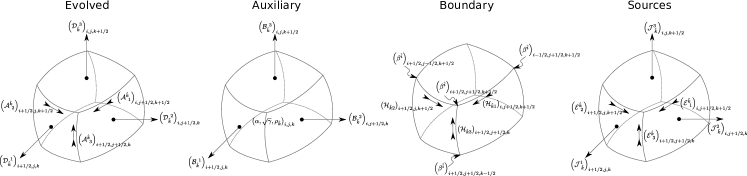
Figure 1: Collocation of variables for a constraint-preserving discretization. These are classified in four categories: ‘evolved’ variables are those obtained by integrating the evolution equations of the scheme, ‘boundary’ variables are those localized at the boundaries of the regions where the evolved variables are defined, and ‘source’ variables are those sharing the same spatial location as the evolved variables. Finally, ‘auxiliary’ variables are those that can be obtained from the evolved variables, but are neither sharing their spatial location nor that of their boundaries.

VII Conclusions

By expressing the equations that govern space-time dynamics in general relativity in the language of exterior calculus and projecting them onto 3-dimensional space-like hypersurfaces, we have obtained a new 3+1 formulation of the field equations of general relativity. This new formulation, which we name dGREM, shows a surprising resemblance to the equations of relativistic MHD and to EM in material media. The system, summarized in Sec. VI, consists of a set of first-order evolution equations, in conservative form, and a set of algebraic, divergence and curl constraints, closed by a set of constitutive relations.

The similarities with 3+1 electrodynamics make explicit some important features of general relativity, such as the global conservation of total energy-momentum currents (in analogy to that of electric current), the fact that both the gravitational and matter energy momentum act as sources of the gravitational field, as well as the energy-momentum exchange between the gravitational and matter sectors.

Additionally, the dGREM formulation exhibits several interesting properties from the point of view of numerical implementations. Being first order and flux-conservative, it is suitable for the application of high-resolution shock-capturing schemes such as finite-volume and finite-element methods. In particular the formulation contains a global conservation equation for the sum of gravitational and “matter” energy-momentum in which source terms have been eliminated, and which opens the possibility of applying techniques such as first-order flux limiting to ensure positivity of energy-momentum densities.

As shown in Sec. VI.2, the expression of the formulation as a set of equations in differential forms permits to integrate them over mesh zones and use Stoke’s theorem to obtain a natural staggered discretization potentially suitable for machine-precision constraint-preserving schemes. One such scheme could potentially reduce the number of evolution variables to a minimum of 21, both by not requiring extra variables to clean the constraints and by making redundant some of the equations.

Although a staggered scheme would enforce at machine-precision both the fulfillment of the Einstein constraints and the conservation of energy-momentum, these advantages may be limited in practice for general relativistic hydrodynamic simulations due to the adoption of a floor model as it is customarily done to handle vacuum regions.

However, these techniques could in principle also be exploited in fully general relativistic N-body simulations, which could recycle the infrastructure developed for PIC simulations of collisionless plasmas, in which both staggered schemes and divergence cleaning techniques have been successfully applied.

In the same way, it is conceivable that resemblance of the form taken by the constraints of this formulation to Gauss’ laws in electromagnetism could present advantages for the computation of initial data by recycling techniques used to solve the Poisson equation.

Finally, another benefit of deriving the system as a set of equations in terms of differential forms and exterior derivatives is that they naturally give relations between quantities evolved inside mesh cells and quantities evaluated at cell boundaries, regardless of the shape of the cells. This makes them particularly suitable for simulations using non-Cartesian coordinates and unstructured meshes.

Finally, the matter sector of the Einstein field equations (including relativistic dissipative fluid dynamics) can be also formulated in the language of differential forms and exterior calculus (Romenski et al., 2020; Peshkov et al., 2019), and thus can be relatively easily incorporated in the constrained transport computational scheme discussed in Sec. VI.2.

Together with the promising properties summarized above, there are still some questions regarding dGREM that need to be answered for a successful numerical implementation. The most important one is perhaps on its hyperbolicity, and how it could depend on gauge choices and on the new degrees of freedom given by spatial rotations of the tetrads between different hypersurfaces.

Other particulars of an actual numerical implementation are still under development, and will be part of a future work.

Appendix A A small primer on differential forms and exterior calculus

We collect here some fundamental results about differential forms and exterior calculus, necessary to follow the derivations in this work. The modern theory of differential forms and exterior calculus stems from the work of Élie Cartan in the first half of the twentieth century, and the literature regarding this field is by now very extensive. For further reading we refer the reader to (Nakahara, 2018; Frauendiener, 2006; Burton, 2003) and references therein, which are the sources this primer is based on. Note that we quote definitions and results in the form they assume in the spacetime of GR, i.e. a 4-dimensional Lorentzian manifold, indicated by the symbol $\mathcal{M}$. We refer the interested reader to the literature for statements valid in more general settings.

A sum of the form

$$\boldsymbol{F}=F_{a}\boldsymbol{\theta}^{a}$$ (117)

is called a $1$-differential form, or simply a $1$-form, and $F_{a}$ are its components. $1$-forms are therefore identical to covariant vectors. More generally, $p$-differential forms (in the following simply $p$-forms) are rank-$p$ totally antisymmetric covariant tensors on $\mathcal{M}$. The differential forms of highest possible degree are $4$-forms, since for higher degrees the antisymmetry requirement would make any differential form vanish identically. $0$-forms are defined as scalar functions on $\mathcal{M}$ (scalar fields).

The set of $p$-forms at a point $P$ of $\mathcal{M}$ forms a $\binom{4}{p}$-dimensional vector space. Therefore the dimensions of the spaces of $0$-, $1$-, $2$-, $3$- and $4$-forms (and the number of components of any form in one of these spaces) are respectively 1, 4, 6, 4, 1.

For the rest of this section, let $\boldsymbol{A}$ and $\boldsymbol{B}$ be generic $p$- and $q-$forms respectively. We define an operation that acts on two such forms to produce a $(p+q)$-form. This is referred to as the exterior product or wedge product, and it is defined as:

$$\boldsymbol{A}\wedge\boldsymbol{B}:=\textnormal{Alt}(\boldsymbol{A}\otimes\boldsymbol{B})\,,$$ (118)

where $\otimes$ is the standard tensor product and $\textnormal{Alt}(\boldsymbol{T})$ denotes is the totally antisymmetric part of the tensor $\boldsymbol{T}$. The components of a the result of the wedge product are therefore:

$$(\boldsymbol{A}\wedge\boldsymbol{B})_{a_{1}\dots a_{p+q}}=$$

$$\frac{1}{(p+q)!}\sum_{P\in S}\text{sgn}(P)A_{a_{P(1)}\dots a_{P(p)}}B_{b_{P(p+1)}\dots b_{P(p+q)}}\,,$$ (119)

where $S$ is the set of all possible permutations of $p+q$ elements, $P$ is one such permutation and $\text{sgn}(P)$ equals $+1$ for even permutations and $-1$ for odd ones. Using a shorthand notation common in the GR literature, this formula can be written as:

$$(\boldsymbol{A}\wedge\boldsymbol{B})_{c_{1}\dots a_{p+q}}=A_{[a_{1}\dots a_{p}}B_{a_{p+1}\dots a_{p+q}]}\,.$$ (120)

The exterior product is associative, and more importantly it satisfies the relation

$$\boldsymbol{A}\wedge\boldsymbol{B}=(-1)^{pq}\boldsymbol{B}\wedge\boldsymbol{A}\,.$$ (121)

This in particular implies that for $1$-forms the exterior product is antisymmetric.

Recall that the set $\boldsymbol{\theta}^{a}$ is a basis of the vector space of $1$-forms. Leveraging the antisymmetry of the exterior product for $1$-forms, it can be seen that the set of elements of the form

$$\boldsymbol{\theta}^{a_{1}}\wedge\dots\wedge\boldsymbol{\theta}^{a_{p}}\,,$$ (122)

i.e. the exterior product of $p$ elements of the basis of $1$-forms, constitutes a basis for the vector space of $p$-forms. For example, a basis for the space of $2$-forms in a 4-dimensional spacetime is

$$\{\boldsymbol{\theta}^{0}\wedge \boldsymbol{\theta}^{1},\boldsymbol{\theta}^{0}\wedge\boldsymbol{\theta}^{2},\boldsymbol{\theta}^{0}\wedge\boldsymbol{\theta}^{3},$$

$$\boldsymbol{\theta}^{1}\wedge\boldsymbol{\theta}^{2},\boldsymbol{\theta}^{1}\wedge\boldsymbol{\theta}^{3},\boldsymbol{\theta}^{2}\wedge\boldsymbol{\theta}^{3}\}\,,$$ (123)

which as noted above has 6 elements.

A $1$-form defines a linear operator acting on vectors and producing a real number, so that the result of a $1$-form $\boldsymbol{F}$ acting on a vector $\boldsymbol{X}$ can be written

$$\boldsymbol{F}(\boldsymbol{X})=F_{a}X^{a}=\langle\boldsymbol{F},\boldsymbol{X}\rangle\,,$$ (124)

where the last equality shows that this is nothing but the interior product between vectors and their duals induced by the metric.

The interior product is instead an operation between a $p$-form and a vector $\boldsymbol{X}$, which gives as result a $(p-1)$-form according to the definition:

$$(\iota_{\boldsymbol{X}}\boldsymbol{A})_{a_{2}\dots a_{p}}:=X^{a_{1}}A_{a_{1}a_{2}\dots a_{p}}\,.$$ (125)

While the inner product and the interior product should not be confused, the latter is in a sense an extension of the former, since $\iota_{\boldsymbol{X}}\boldsymbol{F}=\langle\boldsymbol{X},\boldsymbol{F}\rangle=\boldsymbol{F}(\boldsymbol{X})$.

As stated above, $p$-forms are antisymmetric $(0,p)$-tensors, and as tensors they are acted upon by the standard partial and covariant derivatives. There is however another type of derivation which affects these objects (and is instead not defined for more general tensors). This is called the exterior derivative, and denoted by the symbol $\boldsymbol{d}$. It can be defined by stating that the exterior derivative of a form $\boldsymbol{A}=A_{a_{1}\dots a_{p}}\boldsymbol{\theta}^{a_{1}}\wedge\dots\wedge\boldsymbol{\theta}^{a_{p}}$ is

$$\boldsymbol{d}\boldsymbol{A}=(\partial_{b}A_{a_{1}\dots a_{p}})\boldsymbol{\theta}^{b}\wedge\boldsymbol{\theta}^{a_{1}}\wedge\dots\wedge\boldsymbol{\theta}^{a_{p}}\,.$$ (126)

Since the exterior products automatically antisymmetrize the coefficients, this definition implies that the components of the result can be written as

$$(\boldsymbol{d}\boldsymbol{A})_{ba_{1}\dots a_{p}}=\partial_{[b}A_{a_{1}\dots a_{p}]}\,.$$ (127)

The exterior derivative associates to any $p$-form a $(p+1)$-form, and it clearly does not depend on the metric or on any other additional structure on the manifold. Despite the partial derivative being used in its definition, the components of the exterior derivative form the components of a tensor, i.e. objects obtained by applying it transform as tensors under changes of basis.

Note that as the partial derivative, the exterior derivative is a linear operation, however it exhibits a modified Leibniz rule with respect to the exterior product:

$$\boldsymbol{d}(\boldsymbol{A}\wedge\boldsymbol{B})=\boldsymbol{d}\boldsymbol{A}\wedge\boldsymbol{B}+(-1)^{p}\boldsymbol{A}\wedge\boldsymbol{d}\boldsymbol{B}\,.$$ (128)

Another fundamental property of the exterior derivative, which is leveraged at several points in the present work, is its nilpotency:

$$\boldsymbol{d}\boldsymbol{d}\boldsymbol{A}=0\,.$$ (129)

Note that having defined the exterior derivative and interior product, the definition of the Lie derivative of a $p$-form $\boldsymbol{A}$ along a vector $\boldsymbol{X}$ becomes particularly compact and easy to recall:

$$\mathcal{L}_{\boldsymbol{X}}\boldsymbol{A}=\boldsymbol{d}\iota_{\boldsymbol{X}}\boldsymbol{A}+\iota_{\boldsymbol{X}}\boldsymbol{d}\boldsymbol{A}\,.$$ (130)

This is known as “Cartan’s magic formula”.

There also exists a definition of a exterior covariant derivative, but to state it we need to first introduce so-called tensor-valued differential forms. So far in this section we only have used real-valued differential forms, i.e. form that when acting upon (sets of) vectors return a real value. However in the main text we make extensive use of tensor-valued forms, which return a collection of real values instead. These forms can be seen as collections of real-valued forms, each member of the collection labeled by indices. Such an object are the connection forms $\boldsymbol{\omega}^{a}_{\ b}$, a collection of $1$-forms, defined by

$$\nabla_{\boldsymbol{e}_{a}}\boldsymbol{e}_{b}=\boldsymbol{\omega}^{c}_{\ b}(\boldsymbol{e}_{a})\boldsymbol{e}_{c}\,.$$ (131)

If the connection is chosen as the usual Levi-Civita connection, then $\boldsymbol{\omega}^{\mu}_{\ nu}=\Gamma^{\mu}_{\ \lambda\nu}\boldsymbol{\theta}^{\lambda}$ where $\Gamma^{\mu}_{\ \lambda\nu}$ are the usual Christoffel symbols. In general however the connection forms encode any arbitrary connection.

A few comments are in order. First of all, despite the possibly confusing notation, note that $\boldsymbol{\omega}^{a}_{\ b}$ is not a rank-2 tensor of type $(1,1)$. It is collection of $1$-forms, which becomes apparent by noting that it is defined as the product of the basis $1$-forms and a collection of numbers. Secondly, just as the components of the Christoffel symbols do not transform as the components of a tensor, neither do the components of the object that the connection forms yield when applied to a vector. In this sense the name “tensor-valued form” if applied to the connection forms is a misnomer, since the components of the object yielded by such a form do not, in general, transform as a tensor. The locution “collection of $p$-forms” while possibly less descriptive, is also more appropriate. In light of this, we refer to the indices of the connection $1$-forms in (131) as “non-tensorial” indices. In the main text we deal with collection of forms, some of which are non-tensorial like the connection forms and others instead are proper tensor-valued forms, i.e. their components do transform as those of tensors.

The connection $1$-forms allow us to finally define the exterior covariant derivative of a tensor-valued $p$-form by

$$\boldsymbol{D}\boldsymbol{T}^{a\dots d}_{\hphantom{a\dots d}e\dots h}=\boldsymbol{d}\boldsymbol{T}^{a\dots d}_{\hphantom{a\dots d}e\dots h}+$$

$$+\boldsymbol{\omega}^{a}_{\ i}\wedge\boldsymbol{T}^{i\dots d}_{\hphantom{a\dots d}e\dots h}+\boldsymbol{\omega}^{d}_{\ i}\wedge\boldsymbol{T}^{a\dots i}_{\hphantom{a\dots d}e\dots h}+$$

$$-\boldsymbol{\omega}^{i}_{\ e}\wedge\boldsymbol{T}^{a\dots d}_{\hphantom{a\dots d}i\dots h}-\boldsymbol{\omega}^{i}_{\ h}\wedge\boldsymbol{T}^{a\dots d}_{\hphantom{a\dots d}e\dots i}\,.$$ (132)

Note however that this operation is only defined when applied on a form that is tensor-valued in the strict sense, i.e. when its indices are actually tensorial and transform as the components of a tensor. Under this condition, the indices of the result of applying the covariant exterior derivative will also transform as those of a tensor.

In what follows we go back to real-valued forms. As a consequence of the antisymmetry of differential forms, all the $4$-forms (i.e. the highest possible degree forms in a $4$-dimensional manifold) are multiples of a single $4$-form, called volume form or metric volume element, and defined as

$$\boldsymbol{\varepsilon}=\sqrt{-g}\,\boldsymbol{\theta}^{0}\wedge\boldsymbol{\theta}^{1}\wedge\boldsymbol{\theta}^{2}\wedge\boldsymbol{\theta}^{3}\,.$$ (133)

Its components can be written as

$$\varepsilon_{abcd}=\sqrt{-g}\epsilon_{abcd}\,,$$ (134)

where as anticipated in Sec. II, $g$ is the determinant of the metric and the Levi-Civita symbol $\epsilon_{abcd}$ equals $+1$ or $-1$ depending on whether $(a,b,c,d)$ is an even or an odd permutation of $(0,1,2,3)$. Note also that raising the components of the volume element with the metric results in

$$\varepsilon^{abcd}=-\frac{1}{\sqrt{-g}}\epsilon^{abcd}\,.$$ (135)

It is also useful to note these properties of the volume form and Levi-Civita symbol when restricted to purely spatial, tridimensional hypersurfaces, which are used extensively in the main text:

$$\varepsilon_{0ijk} =-\alpha\varepsilon_{ijk}$$ (136)

$$\varepsilon^{0ijk} =\frac{1}{\alpha}\varepsilon^{ijk}$$ (137)

$$\varepsilon_{ijk} =\sqrt{\gamma}\epsilon_{ijk}$$ (138)

$$\varepsilon^{ijk} =\frac{1}{\sqrt{\gamma}}\epsilon^{ijk}\,.$$ (139)

Furthermore, we note that in a non-coordinate, orthonormal frame, $g=-1$ so that

$$\varepsilon_{\hat{\alpha}\hat{\beta}\hat{\gamma}\hat{\delta}}=\epsilon_{\hat{\alpha}\hat{\beta}\hat{\gamma}\hat{\delta}}\quad\textnormal{and}\quad\varepsilon_{\hat{i}\hat{j}\hat{k}}=\epsilon_{\hat{i}\hat{j}\hat{k}}\,.$$ (140)

Accordingly in such a case (but not in general) we can write the former for the latter and vice versa.

As outlined above the vector space of $p$-forms and that of $(4-p)$-forms have the same dimension. Therefore it is possible to build an isomorphism between these spaces. A very important such isomorphism is the Hodge duality, represented by the symbol $\star$. The components of the Hodge dual can be obtained as

$$(\boldsymbol{\star A})_{a_{p+1}\dots a_{4}}=\varepsilon_{a_{1}\dots a_{p},\,a_{p+1}\dots a_{4}}A^{a_{1}\dots a_{p}}\\$$ (141)

Applying this formula to computing the Hodge dual of $0$-forms, it follows in particular that $\star 1=\boldsymbol{\epsilon}$.

An important property of the Hodge dual is that for any $p$-form

$$\star\star\boldsymbol{A}=(-1)^{1+p(4-p)}\boldsymbol{A}\,,$$ (142)

which implies

$$\star^{-1}\boldsymbol{A}=(-1)^{1+p(4-p)}\star\boldsymbol{A}\,.$$ (143)

Another property of $p$-forms which is fundamental for the present work is that they are natural integrands over $p$-dimensional (sub-)manifolds of $\mathcal{M}$. In particular, if a $p$-dimensional submanifold of $\mathcal{M}$ is further divided into a set of non-overlapping $p$-dimensional regions, a $p$-form $\boldsymbol{A}$ naturally establishes a map from this set to the set of real numbers. If $\mathcal{S}_{1}$ and $\mathcal{S}_{2}$ are such regions, then

$$\boldsymbol{A}[\mathcal{S}_{1}]=\int_{\mathcal{S}_{1}}\boldsymbol{A}$$ (144)

and

$$\boldsymbol{A}[\mathcal{S}_{1}\cup\mathcal{S}_{2}]=\int_{\mathcal{S}_{1}}\boldsymbol{A}+\int_{\mathcal{S}_{2}}\boldsymbol{A}\,.$$ (145)

Note in particular that the integral of $\boldsymbol{\epsilon}$ over a portion of $\mathcal{M}$ is nothing but the volume of that portion, hence the name volume form for $\boldsymbol{\epsilon}$.

We can then state the modern version of Stokes’ theorem, which generalizes the well known theorems of vector calculus by Green, Stokes and Gauss. It allows to relate integrals over a general submanifold $\mathcal{S}$ of $\mathcal{M}$ to integrals over its boundary $\partial\mathcal{S}$

$$\int_{\mathcal{S}}\boldsymbol{d}\boldsymbol{A}=\int_{\partial\mathcal{S}}\boldsymbol{A}\,.$$ (146)

(146) too has a fundamental importance for this work.

Finally, it can be useful to restate standard vector-calculus operators in terms of differential forms and exterior calculus operators, e.g.:

$$\textnormal{grad}(f) =\overrightarrow{\boldsymbol{d}f}\,,$$ (147)

$$\textnormal{div}(\boldsymbol{u}) =-\star^{-1}\boldsymbol{d}\star\widetilde{\boldsymbol{u}}\,,$$ (148)

$$\textnormal{curl}(\boldsymbol{u}) =\overrightarrow{\star\boldsymbol{d}\widetilde{\boldsymbol{u}}}\,.$$ (149)

In these expressions $f$ is a generic scalar field (or equivalently a $0$-form), and $\boldsymbol{u}$ a generic vector; an arrow is used to denote the operation of transforming a differential $1$-form to its dual vector, and a tilde to denote the inverse operation.

Appendix B Hodge dual of the Nester-Witten form in terms of the connection

In order to obtain equation (56), we start from the definition of the Nester-Witten form (27), which can also be written as

$$\boldsymbol{u}_{a}=-\frac{1}{2}\omega^{bc}_{\ \ d}\boldsymbol{\theta}^{d}\wedge\boldsymbol{\Sigma}_{abc}\,.$$ (150)

Using the identity (14), we obtain

$$\boldsymbol{u}_{a}=-\frac{3}{2}\omega^{bc}_{\ \ d}\delta^{d}_{\ [a}\boldsymbol{\Sigma}_{bc]}\,.$$ (151)

Expanding the antisymmetric brackets,

$$\begin{split}\boldsymbol{u}_{a}=-\frac{1}{4}\left[\right.&\omega^{bc}_{\ \ a}\boldsymbol{\Sigma}_{bc}+\omega^{bd}_{\ \ d}\boldsymbol{\Sigma}_{ab}+\omega^{dc}_{\ \ d}\boldsymbol{\Sigma}_{ca}\\ -&\omega^{bc}_{\ \ a}\boldsymbol{\Sigma}_{cb}-\omega^{dc}_{\ \ d}\boldsymbol{\Sigma}_{ac}-\omega^{bd}_{\ \ d}\boldsymbol{\Sigma}_{ba}\left.\right]\,,\end{split}$$ (152)

and renaming indices to factor out $\boldsymbol{\Sigma}_{bc}$,

$$\boldsymbol{u}_{a}=-\frac{1}{2}\left(\omega^{[bc]}_{\ \ \ a}+\delta^{b}_{\ a}\omega^{[cd]}_{\ \ \ d}-\delta^{c}_{\ a}\omega^{[bd]}_{\ \ \ d}\right)\boldsymbol{\Sigma}_{bc}\,.$$ (153)

From the definition of the hypersurface forms (13) and the formula to obtain the components of the Hodge dual (141), it follows that the expression in parenthesis equals the components of $\star\boldsymbol{u}_{a}$, as stated in equation (56).

Appendix C Derivation of evolution equation for $\sqrt{\gamma}$

As mentioned in Section V.4, one can obtain an evolution equation for $\sqrt{\gamma}$ in a conservative form by taking the exterior derivative of the hypersurface form $\boldsymbol{\Sigma}_{\hat{0}}$ orthogonal to $-n_{\mu}$. This form is identical to the Hodge dual of $\boldsymbol{\theta}^{\hat{0}}$, and in a coordinate basis it has components

$$(\boldsymbol{\Sigma_{\hat{0}}})_{\mu\nu\lambda}=-\varepsilon_{\alpha\mu\nu\lambda}n^{\alpha}\,.$$ (154)

Similarly as in Section III, the components of its exterior derivative will take the form of a conservation equation for $n^{\alpha}$,

$$\left(\frac{1}{\sqrt{-g}}\partial_{\mu}\sqrt{-g}n^{\mu}\right)\boldsymbol{\Sigma}=\boldsymbol{d}\boldsymbol{\Sigma_{\hat{0}}}$$ (155)

or taking a single component (for a 4-form, all of them are equal up to a factor $-1$),

$$\partial_{t}\sqrt{\gamma}-\partial_{i}\sqrt{\gamma}\beta^{i}=(\boldsymbol{d}\boldsymbol{\Sigma_{\hat{0}}})_{0123}$$ (156)

To find an expression for the right hand side, we recall the definition of hypersurface forms (13) and write

$$\begin{split}\boldsymbol{\Sigma}_{\hat{0}}=&\varepsilon_{\hat{0}\hat{\mu}\hat{\nu}\hat{\lambda}}\boldsymbol{\theta}^{\hat{\nu}}\wedge\boldsymbol{\theta}^{\hat{\mu}}\wedge\boldsymbol{\theta}^{\hat{\lambda}}\\ =&-\varepsilon_{\hat{i}\hat{j}\hat{k}}\boldsymbol{\theta}^{\hat{i}}\wedge\boldsymbol{\theta}^{\hat{j}}\wedge\boldsymbol{\theta}^{\hat{k}}\,.\end{split}$$ (157)

Now we take the exterior derivative and using the Leibniz rule for the exterior product (128) and the definition of $\boldsymbol{F}^{\hat{a}}$ (72) to obtain

$$\boldsymbol{d}\boldsymbol{\Sigma}_{\hat{0}}=-\varepsilon_{\hat{i}\hat{j}\hat{k}}\boldsymbol{F}^{\hat{i}}\wedge\boldsymbol{\theta}^{\hat{j}}\wedge\boldsymbol{\theta}^{\hat{k}}\,.$$ (158)

For the last step, we need to obtain the component $0123$ of this form in a coordinate frame. This reads

$$\begin{split}(\boldsymbol{d}\boldsymbol{\Sigma}_{\hat{0}})_{0123}=&-\frac{1}{24}\varepsilon_{\hat{i}\hat{j}\hat{k}}F^{\hat{i}}_{\ \hat{\mu}\hat{\nu}}\delta^{\hat{\mu}\hat{\nu}\hat{j}\hat{k}}_{\hat{\alpha}\hat{\beta}\hat{\gamma}\hat{\delta}}A^{\hat{\alpha}}_{\ 0}A^{\hat{\beta}}_{\ 1}A^{\hat{\gamma}}_{\ 2}A^{\hat{\delta}}_{\ 3}\\ =&-\frac{1}{24}\varepsilon_{\hat{i}\hat{j}\hat{k}}F^{\hat{i}}_{\ \hat{\mu}\hat{\nu}}\delta^{\hat{\mu}\hat{\nu}\hat{j}\hat{k}}_{\hat{0}\hat{l}\hat{m}\hat{n}}A^{\hat{0}}_{\ 0}A^{\hat{l}}_{\ 1}A^{\hat{m}}_{\ 2}A^{\hat{n}}_{\ 3}\end{split}$$ (159)

where the renaming of indices follows from the fact that $A^{\hat{0}}_{\ i}=0$, so the lower indices of the $\delta$ will be a permutation of the upper ones only if the remaining indices are different from zero. Since the hatted latin indices cannot take the value $\hat{0}$, many components of the delta are eliminated, and, taking into account the antisymmetry on the last two indices of $F^{\hat{i}}_{\ \hat{\mu}\hat{\nu}}$, we arrive at

$$\begin{split}(\boldsymbol{d}\boldsymbol{\Sigma}_{\hat{0}})_{0123}=&-\frac{1}{12}\varepsilon_{\hat{i}\hat{j}\hat{k}}F^{\hat{i}}_{\ 0\hat{p}}\delta^{\hat{p}\hat{j}\hat{k}}_{\hat{l}\hat{m}\hat{n}}A^{\hat{l}}_{\ 1}A^{\hat{m}}_{\ 2}A^{\hat{n}}_{\ 3}\\ =&-\frac{1}{2}\varepsilon_{\hat{i}\hat{j}\hat{k}}F^{\hat{p}}_{\ 0\hat{p}}A^{\hat{i}}_{\ 1}A^{\hat{j}}_{\ 2}A^{\hat{k}}_{\ 3}\\ =&-\frac{1}{2}\sqrt{\gamma}F^{\hat{p}}_{\ 0\hat{p}}\end{split}$$ (160)

where the second step follows from the fact that $\hat{p}\hat{j}\hat{k}$ can be a permutation of $\hat{i}\hat{j}\hat{k}$ only if $\hat{p}=\hat{i}$ and the third from the definition of the determinant. Now we can evaluate the sum by contracting (80) and then using the constitutive relation (92),

$$(\boldsymbol{d}\boldsymbol{\Sigma}_{\hat{0}})_{0123}=-\frac{1}{2}\sqrt{\gamma}E^{\hat{i}}_{\ \hat{i}}=\frac{5}{2}D_{\hat{k}}^{\ \hat{k}}\,.$$ (161)

Finally, equating (156) and (161), we obtain equation (86).

References

- Abbott et al. (2016) B. P. Abbott, R. Abbott, T. D. Abbott, M. R. Abernathy, F. Acernese, K. Ackley, C. Adams, T. Adams, P. Addesso, R. X. Adhikari, and et al., Phys. Rev. Lett. 116, 061102 (2016), arXiv:1602.03837 [gr-qc] .
- Abbott et al. (2017a) B. P. Abbott, R. Abbott, T. D. Abbott, F. Acernese, K. Ackley, C. Adams, T. Adams, P. Addesso, R. X. Adhikari, V. B. Adya, and et al., Phys. Rev. Lett. 119, 161101 (2017a), arXiv:1710.05832 [gr-qc] .
- Abbott et al. (2017b) B. P. Abbott, R. Abbott, T. D. Abbott, F. Acernese, K. Ackley, C. Adams, T. Adams, P. Addesso, R. X. Adhikari, V. B. Adya, and et al., Astrophys. J. Lett. 848, L12 (2017b), arXiv:1710.05833 [astro-ph.HE] .
- Event Horizon Telescope Collaboration et al. (2019) Event Horizon Telescope Collaboration, K. Akiyama, A. Alberdi, W. Alef, K. Asada, R. Azulay, A.-K. Baczko, D. Ball, M. Baloković, J. Barrett, and et al., Astrophys. J. Lett. 875, L4 (2019), arXiv:1906.11241 [astro-ph.GA] .
- Event Horizon Telescope Collaboration et al. (2021) Event Horizon Telescope Collaboration, K. Akiyama, J. C. Algaba, A. Alberdi, W. Alef, R. Anantua, K. Asada, R. Azulay, A.-K. Baczko, D. Ball, and et al., Astrophys. J. Lett. 910, L12 (2021), arXiv:2105.01169 [astro-ph.HE] .
- Pretorius (2005) F. Pretorius, Phys. Rev. Lett. 95, 121101 (2005), arXiv:gr-qc/0507014 [gr-qc] .
- Garfinkle (2002) D. Garfinkle, Phys. Rev. D 65, 044029 (2002), arXiv:gr-qc/0110013 [gr-qc] .
- Lindblom et al. (2006) L. Lindblom, M. A. Scheel, L. E. Kidder, R. Owen, and O. Rinne, Classical and Quantum Gravity 23, S447 (2006), arXiv:gr-qc/0512093 [gr-qc] .
- Winicour (2012) J. Winicour, Living Reviews in Relativity 15, 2 (2012).
- Frauendiener and Friedrich (2002) J. Frauendiener and H. Friedrich, The Conformal Structure of Space-Time - Geometry, Analysis, Numerics (Springer, Berlin, Heidelberg, 2002).
- Hus (2003) Current Trends in Relativistic Astrophysics - Theoretical, Numerical, Observational, Vol. 617 (Springer-Verlag Berlin Heidelberg, 2003).
- Cordero-Carrión et al. (2008) I. Cordero-Carrión, J. M. Ibáñez, E. Gourgoulhon, J. L. Jaramillo, and J. Novak, Phys. Rev. D 77, 084007 (2008), arXiv:0802.3018 [gr-qc] .
- Alcubierre (2008) M. Alcubierre, Introduction to 3+1 Numerical Relativity (Oxford University Press, Oxford, UK, 2008).
- Rezzolla and Zanotti (2013) L. Rezzolla and O. Zanotti, Relativistic Hydrodynamics (2013).
- Baumgarte and Shapiro (2010) T. W. Baumgarte and S. L. Shapiro, Numerical Relativity: Solving Einstein’s Equations on the Computer (2010).
- Cook (2000) G. B. Cook, Living Reviews in Relativity 3, 5 (2000), arXiv:gr-qc/0007085 [gr-qc] .
- Arnowitt et al. (1959) R. Arnowitt, S. Deser, and C. W. Misner, Physical Review 116, 1322 (1959).
- York (1979) J. York, J. W., in Sources of Gravitational Radiation, edited by L. L. Smarr (1979) pp. 83–126.
- Shibata and Nakamura (1995) M. Shibata and T. Nakamura, Phys. Rev. D 52, 5428 (1995).
- Baumgarte and Shapiro (1998) T. W. Baumgarte and S. L. Shapiro, Phys. Rev. D 59, 024007 (1998), arXiv:gr-qc/9810065 [gr-qc] .
- Brown (2009) J. D. Brown, Phys. Rev. D 79, 104029 (2009), arXiv:0902.3652 [gr-qc] .
- Beyer and Sarbach (2004) H. Beyer and O. Sarbach, Phys. Rev. D 70, 104004 (2004), arXiv:gr-qc/0406003 [gr-qc] .
- Alic et al. (2012) D. Alic, C. Bona-Casas, C. Bona, L. Rezzolla, and C. Palenzuela, Phys. Rev. D 85, 064040 (2012), arXiv:1106.2254 [gr-qc] .
- Brown et al. (2012) J. D. Brown, P. Diener, S. E. Field, J. S. Hesthaven, F. Herrmann, A. H. Mroué, O. Sarbach, E. Schnetter, M. Tiglio, and M. Wagman, Phys. Rev. D 85, 084004 (2012), arXiv:1202.1038 [gr-qc] .
- Dedner et al. (2002) A. Dedner, F. Kemm, D. Kröner, C. D. Munz, T. Schnitzer, and M. Wesenberg, J. Comput. Phys. 175, 645 (2002).
- Bona et al. (2003) C. Bona, T. Ledvinka, C. Palenzuela, and M. Žáček, Phys. Rev. D 67, 104005 (2003), arXiv:gr-qc/0302083 [gr-qc] .
- Bernuzzi and Hilditch (2010) S. Bernuzzi and D. Hilditch, Phys. Rev. D 81, 084003 (2010), arXiv:0912.2920 [gr-qc] .
- Alic et al. (2013) D. Alic, W. Kastaun, and L. Rezzolla, Phys. Rev. D 88, 064049 (2013), arXiv:1307.7391 [gr-qc] .
- Gundlach et al. (2005) C. Gundlach, J. M. Martin-Garcia, G. Calabrese, and I. Hinder, Class. Quant. Grav. 22, 3767 (2005), arXiv:gr-qc/0504114 .
- Griffiths (2017) D. J. Griffiths, Introduction to Electrodynamics, 4th ed. (Cambridge University Press, 2017).
- Jackson (1998) J. D. Jackson, Classical electrodynamics; 3nd ed. (Wiley, New York, NY, 1998).
- Pretorius (2006) F. Pretorius, Class. Quant. Grav. 23, S529 (2006), arXiv:gr-qc/0602115 .
- Dumbser et al. (2018) M. Dumbser, F. Guercilena, S. Köppel, L. Rezzolla, and O. Zanotti, Phys. Rev. D 97, 084053 (2018), arXiv:1707.09910 [gr-qc] .
- Brown et al. (2012) J. D. Brown, P. Diener, S. E. Field, J. S. Hesthaven, F. Herrmann, A. H. Mroue, O. Sarbach, E. Schnetter, M. Tiglio, and M. Wagman, Phys. Rev. D 85, 084004 (2012), arXiv:1202.1038 [gr-qc] .
- Teukolsky (2016) S. A. Teukolsky, J. Comput. Phys. 312, 333 (2016), arXiv:1510.01190 [gr-qc] .
- Hébert et al. (2018) F. Hébert, L. E. Kidder, and S. A. Teukolsky, Phys. Rev. D 98, 044041 (2018), arXiv:1804.02003 [gr-qc] .
- Bhattacharyya et al. (2021) M. K. Bhattacharyya, D. Hilditch, K. Rajesh Nayak, S. Renkhoff, H. R. Rüter, and B. Brügmann, Phys. Rev. D 103, 064072 (2021), arXiv:2101.12094 [gr-qc] .
- Dumbser et al. (2020) M. Dumbser, F. Fambri, E. Gaburro, and A. Reinarz, Journal of Computational Physics 404, 109088 (2020), arXiv:1909.03455 [math.NA] .
- Yee (1966) K. Yee, IEEE Trans. Antennas Propag. 14, 302 (1966).
- Evans and Hawley (1988) C. Evans and J. Hawley, Astrophys. J. 332, 659 (1988).
- Meier (2003) D. L. Meier, Astrophys. J. 595, 980 (2003).
- Frauendiener (2006) J. Frauendiener, Class. Quantum Gravity 23, S369 (2006).
- Dumbser et al. (2017) M. Dumbser, I. Peshkov, E. Romenski, and O. Zanotti, Journal of Computational Physics 348, 298 (2017), arXiv:1612.02093 .
- Etienne et al. (2015) Z. B. Etienne, V. Paschalidis, R. Haas, P. Mösta, and S. L. Shapiro, Class. Quant. Grav. 32, 175009 (2015), arXiv:1501.07276 [astro-ph.HE] .
- Porth et al. (2016) O. Porth, H. Olivares, Y. Mizuno, Z. Younsi, L. Rezzolla, M. Moscibrodzka, H. Falcke, and M. Kramer, (2016), 10.1186/s40668-017-0020-2, arXiv:1611.09720 [gr-qc] .
- Stone et al. (2020) J. M. Stone, K. Tomida, C. J. White, and K. G. Felker, Astrophysical Journal Supplement 249, 4 (2020), arXiv:2005.06651 [astro-ph.IM] .
- Mocz et al. (2014) P. Mocz, M. Vogelsberger, and L. Hernquist, Mon. Not. Roy. Astron. Soc. 442, 43 (2014), arXiv:1402.5963 [astro-ph.IM] .
- Hesthaven and Warburton (2008) J. S. Hesthaven and T. Warburton, Nodal Discontinuous Galerkin Methods - Algorithms, Analysis, and Applications (Springer, New York, NY, 2008).
- Toro (2009) E. F. Toro, Riemann Solvers and Numerical Methods for Fluid Dynamics (Springer-Verlag Berlin Heidelberg, 2009).
- Szabados (1992) L. B. Szabados, Class. Quantum Gravity 9, 2521 (1992).
- Frauendiener (1990) J. Frauendiener, Gen. Relativ. Gravit. 22, 1423 (1990).
- Frittelli (1997) S. Frittelli, Phys. Rev. D - Part. Fields, Gravit. Cosmol. 55, 5992 (1997).
- Clough (2021) K. Clough, Class. Quant. Grav. 38, 167001 (2021), arXiv:2104.13420 [gr-qc] .
- Gammie et al. (2003) C. F. Gammie, J. C. McKinney, and G. Toth, Astrophys. J. 589, 444 (2003), arXiv:astro-ph/0301509 .
- Hu et al. (2013) X. Y. Hu, N. A. Adams, and C.-W. Shu, Journal of Computational Physics 242, 169 (2013), arXiv:1203.1540 [physics.flu-dyn] .
- Wu (2017) K. Wu, Phys. Rev. D 95, 103001 (2017), arXiv:1610.06274 [math.NA] .
- Wu and Tang (2018) K. Wu and H. Tang, Zeitschrift Angewandte Mathematik und Physik 69, 84 (2018), arXiv:1709.05838 [math.NA] .
- Carroll (2004) S. M. Carroll, Spacetime and geometry. An introduction to general relativity (2004).
- Wald (1984) R. M. Wald, General relativity (1984).
- Aldrovandi and Pereira (2013) R. Aldrovandi and J. G. Pereira, Teleparallel Gravity, Vol. 173 (2013).
- Romenski et al. (2020) E. Romenski, I. Peshkov, M. Dumbser, and F. Fambri, Philosophical Transactions of the Royal Society A: Mathematical, Physical and Engineering Sciences 378, 20190175 (2020), arXiv:1910.03298 .
- Peshkov et al. (2019) I. Peshkov, E. Romenski, and M. Dumbser, Continuum Mechanics and Thermodynamics 31, 1517 (2019), arXiv:1810.03761 .
- Nakahara (2018) M. Nakahara, Geometry, Topology and Physics (CRC Press, 2018).
- Burton (2003) D. A. Burton, Theor. App. Mech. 30, 85 (2003).