Multipartite spatial entanglement generated by concurrent nonlinear processes

Abstract

Continuous variables multipartite entanglement is a key resource for quantum technologies. This works considers the multipartite entanglement generated in separated spatial modes of the same light beam by three different parametric sources: a standard $\chi^{(2)}$ medium pumped by two pumps, a single-pump nonlinear photonic crystal, and a doubly pumped nonlinear photonic crystal. These sources have in common the coexistence of several concurrent nonlinear processes in the same medium, which allows the generation of non-standard 3 and 4-mode couplings. We test the genuine nature of the multipartite entangled states thereby generated in a common framework, using both criteria based on proper bounds for the variances of nonlocal observables and on the positive partial transpose criterion. The relative simplicity of these states allows a (hopefully) useful comparison of the different inseparability tests.

Version

Introduction

In optics, the most efficient sources of quantum states are nonlinear processes, such as parametric down-conversion (PDC), that generate photons in pairs. In the continuous-variable regime this mechanism naturally leads to a bipartite Einstein-Podosky-Rosen (EPR) entanglement, involving the phase quadratures of independent couples of modes of the radiation field, or to squeezed states, depending whether the detection process separates or not the photons in the pair. On the other side, photonic states in which entanglement is shared by more than two physical modes are becoming more and more an attractive resource for continuous variable quantum information. A prominent examples is that of measurement-based quantum computation [1, 2], which requires to generate multipartite entangled cluster states [3, 4] in a controlled and re-configurable way. Multipartite entanglement may also enable multiparty quantum communication protocols [5], as secret quantum sharing [6], or can be used in quantum metrology for distributed quantum sensing [7].

The traditional method to transform the bipartite entanglement typical of parametric processes into a multiparty entanglement is sequential, and is based on generating several squeezed state by independent PDC processes and then mixing them into a network of passive optical elements (see e.g. [8, 9, 10]). Multipartite entanglement may be also realized by cascaded nonlinearities [11]. Alternatively, a powerful approach is the parallel generation of a multipartite entanglement among different light modes that copropagate in the same beam. Continuous variable cluster states have been successfully generated in the spectral structure of the frequency comb of a single optical parametric oscillator [12, 13], or of a synchronously pumped optical parametric oscillator [14, 15]. Spatial encoding , which is naturally attractive, has been in comparison less explored, with a recent proposal exploiting an array of nonlinear waveguides [16] interacting with evanescent coupling, which mixes squeezing and entanglement.

This work stems from some recent publications [17, 18, 19, 20, 21, 22], which showed the possibility of generating a multipartite coupling - the prerequisite for multiparty entanglement - among separate spatial modes copropagating in the same beam, by properly engineered parametric processes. The present work will not deal with the physics of the optical sources, extensively described in Refs. [17, 18, 19, 20, 21, 22], but will focus on the characterization and possibly on the quantification of the multipartite entanglement thereby produced.

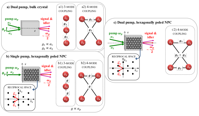
Figure 1: Parametric sources of multipartite spatial entanglement. a) Standard $\chi^{(2)}$ medium pumped by two noncollinear beams of amplitudes $\alpha_{1}$ and $\alpha_{2}$. b) Hexagonally poled NPC, pumped by a single pump $\alpha_{p}$, where two non collinear processes are sustained by vectors $\vec{G}_{1}$ and $\vec{G}_{2}$ of the reciprocal lattice. c) Doubly-pumped NPC, where four processes coexist. The graphs describe the multi-mode coupling generated in specific sets of spatio-temporal modes, in normal conditions [ a1) and b1)] or under special resonance conditions [a2), b2) and c2)] (see text). The couplings $g_{j}\propto\alpha_{j}$, while $g\propto\alpha_{p}$

Figure 1 summarizes the optical schemes that will be considered, along with the states generated by each of them. In Fig.1a, the medium is a standard $\chi^{(2)}$ crystal, but the beam that feeds the process is engineered in the form of two slightly non collinear modes, which determines a transverse modulation of the pumping profile. In the case of Fig.1b the pump is a single-mode beam, but the medium is a nonlinear photonic crystal (NPC) [23], whose $\chi^{(2)}$ response is artificially modulated according to a two-dimensional poling pattern. The common feature of these apparently disparate sources is the coexistence inside the same medium of two concurrent nonlinear processes, which mutually reinforce during propagation, and the existence of spatio-temporal modes of the fluorescence radiation shared by both processes. These constitute an infinite set of bright modes [20, 21], characterized by the non-standard 3-mode coupling schematically depicted by the graphs a1) and b1). Under special conditions, a transition to the linear 4-mode coupling of graphs a2) and b2) can take place [17, 20, 18, 21]. The third example is a mixture of the other two, corresponding to a nonlinear photonic crystal pumped by two noncollinear optical modes. In this case, four nonlinear processes coexist in the same medium, and under particular resonance conditions give rise to the square coupling in the graph c2) [19, 22].

The paper has two main parts. In the first one, following previous literature [24, 25, 26, 27, 28, 29, 30, 11, 31, 32] we set the machinery for describing continuos variable multipartite entanglement and we establish the general criteria that will be used in the second part for characterizing our states. We shall use two methods: the first one, in the spirit of [33, 29], requires setting proper bounds for the variances of nonlocal observables of the system, that when violated certify the entanglement of the state. Our inequalities have nothing substantially new compared to others derived and used in existing literature[29, 31, 32]. However, they have the advantage of being particularly simple and general, and of having the compact form of Heisenberg-like inequalities [see Eq.(14)]. Along with them, we also suggest a viable strategy to identify the nonlocal observables best suited to test the inseparability of a given Gaussian state, based on its Bloch-Messiah decomposition [34]. Due to the relative simplicity of our states, we have full access to their covariance matrix, which gives the possibility of using more powerful inseparability tests directly based on the positive partial transpose criterion [24, 25, 26]. This allows a (hopefully) instructive comparison between the two kinds of inseparability tests.

I CV Multipartite entanglement

Let us start by fixing the formalism and introducing the basic concepts. We consider a system of N optical modes, with bosonic annihilation an creation operators $\hat{a}_{j},\hat{a}_{j}^{\dagger}$ ($j=1,..N$). Hermitian quadrature operators are defined as $\hat{X}_{j}=\hat{a}_{j}+\hat{a}_{j}^{\dagger}$, $\hat{Y}_{j}=\frac{1}{i}(\hat{a}_{j}-\hat{a}_{j}^{\dagger})$, with commutator $\left[\hat{X}_{j},\hat{Y}_{k}\right]=2i\delta_{j,k}$. By introducing the 2N-dimensional vector

$$\hat{\boldsymbol{Q}}=\left(\hat{X}_{1},...,\hat{X}_{N},\hat{Y}_{1},...,\hat{Y}_{N}\right)^{\intercal}\,,$$ (1)

the fundamental commutation relations take the compact form:

$$\left[\hat{Q}_{\alpha},\hat{Q}_{\beta}\right]=2i\Omega_{\alpha\beta}$$ (2)

where $\boldsymbol{\Omega}$ is the $2N\times 2N$ symplectic form $\boldsymbol{\Omega}=\begin{pmatrix}\mathbb{0}_{N}&\mathbb{1}_{N}\\ -\mathbb{1}_{N}&\mathbb{0}_{N}\end{pmatrix}$, with $\mathbb{1}_{N}$ and $\mathbb{0}_{N}$ being the identity and null matrix in N-dimensions . Each state $\hat{\rho}$ of the system can be associated with a covariance matrix, containing the second order moments of quadrature operators in symmetric ordering:

$$V_{\alpha\beta}=\left\langle\left\{\delta\hat{Q}_{\alpha},\delta\hat{Q}_{\beta}\right\}\right\rangle=\mathrm{Tr}\left\{\frac{1}{2}(\delta\hat{Q}_{\alpha}\delta\hat{Q}_{\beta}+\delta\hat{Q}_{\beta}\delta\hat{Q}_{\alpha})\hat{\rho}\right\}$$ (3)

where $\delta\hat{Q}_{j}=\hat{Q}_{j}-\langle\hat{Q}_{j}\rangle$. Gaussian states, in particular, are uniquely determined by their covariance matrix, a part from a displacement in phase space, inessential for the entanglement. A legitimate covariance matrix must be real, symmetric and must satisfy the condition:

$$\boldsymbol{V}+i\boldsymbol{\Omega}\geq 0$$ (4)

meaning that the Hermitian matrix $\boldsymbol{V}+i\boldsymbol{\Omega}$ has non-negative eigenvalues (the same clearly holds true for the complex conjugate $\boldsymbol{V}-i\boldsymbol{\Omega}$, and for the covariance $\boldsymbol{V}$ itself). This condition is a straightforward consequence of the positivity of the density operator $\hat{\rho}$, and of the commutation relation (2), because it ensures that any operator of the form $\hat{\xi}=\sum_{\alpha}c_{\alpha}\delta\hat{Q}_{\alpha}$, where $c_{\alpha}$ are complex coefficients, satisfies

$$\langle\hat{\xi}^{\dagger}\hat{\xi}\rangle=\sum_{\alpha,\beta}c_{\beta}^{*}c_{\alpha}\langle\delta\hat{Q}_{\alpha}\delta\hat{Q}_{\beta}\rangle=\sum_{\alpha,\beta}c_{\beta}^{*}c_{\alpha}\left\langle\left\{\delta\hat{Q}_{\alpha},\delta\hat{Q}_{\beta}\right\}+\frac{1}{2}\left[\hat{Q}_{\alpha},\hat{Q}_{\beta}\right]\right\rangle=\boldsymbol{c}^{\dagger}\left(\boldsymbol{V}+i\boldsymbol{\Omega}\right)\boldsymbol{c}\geq 0$$

for any 2N-dimensional vector of complex numbers $\boldsymbol{c}^{\dagger}=(c_{1}^{*},..,c^{*}_{2N})$, including the eigenvectors of the matrix $\boldsymbol{V}+i\boldsymbol{\Omega}$, whose eigenvalues are therefore non-negative. The condition (4) is often expressed in the equivalent form (see e.g. [30]).

$$\mathrm{Eigen}_{+}\left[i\boldsymbol{\Omega}\boldsymbol{V}\right]\geq 1$$ (5)

where $\mathrm{Eigen}_{+}[\cdot]$ denotes the positive eigenvalues of $i\boldsymbol{\Omega}\boldsymbol{V}$, which form the so-called symplectic spectrum $\boldsymbol{\nu}=\{\nu_{1},\nu_{2}\ldots\nu_{N}\}$ of the covariance matrix. The inequality (4) implies that for a legitimate covariance matrix $\nu_{i}\geq 1$ , $\forall i=1,\ldots,N$ (see appendix A.A for details).

The inequalities (4) and (5) can be considered as a general expressions of the Heinsenberg uncertainty relations, which bound the variances of pairs of observables. If we focus on the simplest type of non-local observables, i.e. linear combinations of the quadrature operators of the modes

$$\hat{\eta}({\mathbf{d}})=\sum_{\alpha}d_{\alpha}\hat{Q}_{\alpha},$$ (6)

$$\hat{\eta}({\mathbf{d}}^{\prime})=\sum_{\alpha}d^{\prime}_{\alpha}\hat{Q}_{\alpha},$$

where ${\mathbf{d}}=(d_{1},d_{2}\ldots d_{2N})^{\intercal}$, ${\mathbf{d}}^{\prime}=(d^{\prime}_{1},d^{\prime}_{2}\ldots d^{\prime}_{2N})^{\intercal}$ are vectors of real coefficients, their variances must satisfy the following Heisenberg bound:

$$\left\langle\delta\hat{\eta}^{2}({\mathbf{d}})\right\rangle+\left\langle\delta\hat{\eta}^{2}({\mathbf{d}}^{\prime})\right\rangle \geq 2\sqrt{\left\langle\delta\hat{\eta}^{2}({\mathbf{d}})\right\rangle}\sqrt{\left\langle\delta\hat{\eta}^{2}({\mathbf{d}}^{\prime})\right\rangle}$$ (7)

$$\geq\left|\left\langle\left[\delta\hat{\eta}({\mathbf{d}}),\delta\hat{\eta}({\mathbf{d}}^{\prime})\right]\right\rangle\right|$$

As well known, these inequalities are a purely mathematical consequence of the positivity of the density operator $\hat{\rho}$, and of the fact that $\hat{\eta}({\mathbf{d}})$ and $\hat{\eta}({\mathbf{d}}^{\prime})$ are Hermitian operator (observables). Indeed it is based on the Cauchy–Schwarz inequality: ${\left\langle\delta\hat{\eta}^{2}({\mathbf{d}})\right\rangle}{\left\langle\delta\hat{\eta}^{2}({\mathbf{d}}^{\prime})\right\rangle}\geq\left|\left\langle\delta\hat{\eta}({\mathbf{d}})\delta\hat{\eta}({\mathbf{d}}^{\prime})\right\rangle\right|^{2}$, and on the inequality $\left|\left\langle\delta\hat{\eta}({\mathbf{d}})\delta\hat{\eta}({\mathbf{d}}^{\prime})\right\rangle\right|=\left|{\mathbf{d}}^{\intercal}(\boldsymbol{V}+i\boldsymbol{\Omega}){\mathbf{d}}^{\prime}\right|\geq\left|{\mathbf{d}}^{\intercal}\boldsymbol{\Omega}\,{\mathbf{d}}^{\prime}\right|=\frac{1}{2}\left|\left\langle\left[\delta\hat{\eta}({\mathbf{d}}),\delta\hat{\eta}({\mathbf{d}}^{\prime})\right]\right\rangle\right|$, which in turn is a straightforward consequence of the fact that ${\mathbf{d}}$ and ${\mathbf{d}}^{\prime}$ are real vectors.
Notice also that the bound for the product of variances is stronger than the one for the sum , because the inequality in the first line of the formula(7) holds strictly unless the two variances are equal.

I.A The PPT criterion in phase space

We consider now the problem of separability of the state with respect to a given bipartition. Let us consider a partition of the N modes into two subgroups $A=\{j_{1},j_{2}\ldots j_{k}\}$ (Alice) and $B=\{m_{1},m_{2}\ldots m_{N-k}\}=A^{C}$ (Bob). We call A-separable those states that can be written in the form $\hat{\rho}=\sum_{n}P_{n}\hat{\rho}_{n}^{(\mathrm{A})}\otimes\hat{\rho}_{n}^{(\mathrm{B})}$, where $P_{n}\geq 0$, and $\hat{\rho}_{n}^{(\mathrm{A})}$ and $\hat{\rho}_{n}^{(\mathrm{B})}$ are density operators on Alice and Bob subspaces.
The Peres-Horodecki [24, 25] Positive Partial Transpose (PPT) criterion establishes that for any A-separable state the operator $\hat{\rho}^{\mathsf{\,\scriptscriptstyle PT(A)}}$ obtained by partial transposition of its density operator with respect to the degrees of freedom of subsystem A is still a legitimate density operator. The existence of a negative partial transpose density operator is thus a sufficient criterion for assessing the A-entanglement of the state, and becomes also necessary for the $\{j_{1}\}\times\{m_{1},..m_{N-1}\}$ partitions of Gaussian states [26, 27]. For the continuous variable systems of interest for this work, an elegant and useful translation of the PPT criterion to phase-space has been performed by Simon [26], who showed that in phase-space the partial transposition corresponds to a mirror reflection of all the Y-quadratures of Alice’s modes. Mathematically, this amounts to a transformation of the covariance matrix of the state, by means of the unitary matrix

$$\boldsymbol{\Gamma}_{A}=\mathrm{diag}\{1,1,\ldots\underset{\underset{N+j_{1}}{\downarrow}}{-1}\ldots\underset{\underset{N+j_{2}}{\downarrow}}{-1}\ldots\underset{\underset{N+j_{k}}{\downarrow}}{-1}\}$$ (8)

which changes the sign of the Y-quadratures of modes $j_{1},j_{2}\ldots j_{k}$ of the set A. The PPT criterion for continuous variables [26, 27] establishes that for any A-separable state the matrix

$$\boldsymbol{V}^{\mathsf{\,\scriptscriptstyle PT(A)}}=\boldsymbol{\Gamma}_{A}\boldsymbol{V}\boldsymbol{\Gamma}_{A}$$ (9)

is still a legitimate covariance matrix, which implies

$$\boldsymbol{V}^{\mathsf{\,\scriptscriptstyle PT(A)}}+i\boldsymbol{\Omega}\geq 0$$ (10)

or, alternatively

$$\mathrm{Eigen}_{+}\left[i\boldsymbol{\Omega}\boldsymbol{V}^{\mathsf{\,\scriptscriptstyle PT(A)}}\right]\geq 1$$ (11)

The conditions (10) or (11) provide powerful means to test the entanglement of the state with respect to the partition $A$: whenever a negative eigenvalue of $\boldsymbol{V}^{\mathsf{\,\scriptscriptstyle PT(A)}}+i\boldsymbol{\Omega}$ appears (or a symplectic eigenvalue of $\boldsymbol{V}^{\mathsf{\,\scriptscriptstyle PT(A)}}$ is smaller than 1), then $\hat{\rho}^{\mathsf{\,\scriptscriptstyle PT(A)}}$ is not a physical state, which implies that $\hat{\rho}$ is not A-separable. Clearly, such a test requires the access to the full covariance matrix of the state, which is often not a viable route in experiments because of the large number of measurements required.

I.B Criteria based on variances of nonlocal observables

Simon [26] proposed a somehow more accessible use of the PPT criterion, that was subsequently applied to various examples of multipartite CV entanglement [29, 11, 31], and systematically generalized by the work in [32]. We propose here a simpler version of the general criteria described in [32], sufficient for characterizing the states of interest in this work.

The Heisenberg inequalities (7) hold for any physical state. A-separable states conversely impose stronger bounds, originating from their positive partial transpose. Because of the equivalence between the partial transposition of the density operator and the mirror reflection of the Y-quadratures of Alice, the variances of each pair of linear combinations of mode quadratures $\hat{\eta}({\mathbf{d}})$ and $\hat{\eta}({\mathbf{d}}^{\prime})$ satisfy the relation:

$$\left\langle\delta\hat{\eta}^{2}({\mathbf{d}})\right\rangle_{\hat{\rho}}+\left\langle\delta\hat{\eta}^{2}({\mathbf{d}}^{\prime})\right\rangle_{\hat{\rho}}=\left\langle\delta\hat{\eta}^{2}(\boldsymbol{\Gamma}_{A}{\mathbf{d}})\right\rangle_{\hat{\rho}^{\mathsf{\,\scriptscriptstyle PT(A)}}}+\left\langle\delta\hat{\eta}^{2}(\boldsymbol{\Gamma}_{A}{\mathbf{d}}^{\prime})\right\rangle_{\hat{\rho}^{\mathsf{\,\scriptscriptstyle PT(A)}}}$$ (12)

where $\left\langle\cdot\right\rangle_{\hat{w}}=\mathrm{Tr}\{\cdot\hat{w}\}$, $\hat{\rho}^{\mathsf{\,\scriptscriptstyle PT(A)}}$ is the partial transpose (with respect to Alice’s set) of the density operator, and $\boldsymbol{\Gamma}_{A}$ is the mirror reflection described by Eq.(8). For A-separable states $\hat{\rho}^{\mathsf{\,\scriptscriptstyle PT(A)}}$ is a valid density operator, so that the r.h.s of Eq.(12) must satisfy a Heisenberg bound analogue to that of Eq.(7), which is a purely algebraic consequence of the positivity of the density operator. Therefore, in A-separable states the variances of observables are subject to the additional bound

$$\left\langle\delta\hat{\eta}^{2}({\mathbf{d}})\right\rangle+\left\langle\delta\hat{\eta}^{2}({\mathbf{d}}^{\prime})\right\rangle \geq 2\left|{\mathbf{d}}^{\intercal}\boldsymbol{\Gamma}_{A}\boldsymbol{\Omega}\,\boldsymbol{\Gamma}_{A}{\mathbf{d}}^{\prime}\right|$$ (13a)

In a similar way, the product of variances in A-separable states are constrained to

$$\sqrt{\left\langle\delta\hat{\eta}^{2}({\mathbf{d}})\right\rangle\left\langle\delta\hat{\eta}^{2}({\mathbf{d}}^{\prime})\right\rangle} \geq\left|{\mathbf{d}}^{\intercal}\boldsymbol{\Gamma}_{A}\boldsymbol{\Omega}\,\boldsymbol{\Gamma}_{A}{\mathbf{d}}^{\prime}\right|$$ (13b)

Actually, equations (13a) and (13b) are just an example of the general criteria described in [32], which involve any kind of functional of nonlocal observables. From the definition of $\hat{\eta}$ in Eq.(6), we notice that $\left[\delta\hat{\eta}(\boldsymbol{\Gamma}_{A}{\mathbf{d}}),\delta\hat{\eta}(\boldsymbol{\Gamma}_{A}{\mathbf{d}}^{\prime})\right]=2i(\boldsymbol{\Gamma}_{A}{\mathbf{d}})^{\intercal}\boldsymbol{\Omega}\,\boldsymbol{\Gamma}_{A}{\mathbf{d}}^{\prime}$, so that Eqs.(13a) and (13b) can be recast in the more expressive form:

$$\left\langle\delta\hat{\eta}^{2}({\mathbf{d}})\right\rangle+\left\langle\delta\hat{\eta}^{2}({\mathbf{d}}^{\prime})\right\rangle \geq 2\sqrt{\left\langle\delta\hat{\eta}^{2}({\mathbf{d}})\right\rangle\left\langle\delta\hat{\eta}^{2}({\mathbf{d}}^{\prime})\right\rangle}$$ (14)

$$\geq\left|\left\langle\left[\delta\hat{\eta}(\boldsymbol{\Gamma}_{A}{\mathbf{d}}),\delta\hat{\eta}(\boldsymbol{\Gamma}_{A}{\mathbf{d}}^{\prime})\right]\right\rangle\right|$$

This inequality has the same form as the Heisenberg relation (7), but the lower bound is determined by the commutator between the mirrored variables. Thus we can say that the uncertainties of observables in separable states are constrained not only by their commutator, as in standard Heisenberg uncertainty relations, but also by the commutators of the mirrored observables. The inequality (14) has the further advantage of not depending on the numerical value of the commutator (often a source of confusion because of the different definitions of $\hat{X},\hat{Y}$ adopted by various authors), and will be systematically used in the next sections of this work.

If the nonlocal variables $\hat{\eta}({\mathbf{d}})$ and $\hat{\eta}({\mathbf{d}}^{\prime})$ are properly chosen, Eq.(14) jointly with the Heisenberg inequality (7), may provide a stronger bound than Eq. (7) alone, obeyed by all the states. A simple example is that of Duan criterion [33] for bipartite entanglement between two bosonic modes $\hat{a}_{1}$ and $\hat{a}_{2}$. Let us consider the nonlocal variables $\hat{\eta}=\frac{1}{\sqrt{2}}\left(s\hat{X}_{1}-\frac{1}{s}\hat{X}_{2}\right)$ and $\hat{\eta}^{\prime}=\frac{1}{\sqrt{2}}\left(s\hat{Y}_{1}+\frac{1}{s}\hat{Y}_{2}\right)$, where $s$ is a real number. In any state, the sum of their uncertainties cannot be below the Heisenberg bound $\left|\left[\hat{\eta},\hat{\eta}^{\prime}\right]\right|=|s^{2}-\frac{1}{s^{2}}|$, which vanishes for s=1. Conversely, separable states needs to respect the stronger bound represented by the commutator of mirrored variables $\left\langle\delta\hat{\eta}^{2}\right\rangle+\left\langle\delta\hat{\eta}^{\prime 2}\right\rangle\geq\frac{1}{2}\left|\left[s\hat{X}_{1}-\frac{1}{s}\hat{X}_{2},s\hat{Y}_{1}-\frac{1}{s}\hat{Y}_{2}\right]\right|=s^{2}+\frac{1}{s^{2}}$. Therefore, violation of this bound is a sufficient condition for the entanglement of any bipartite continuous variable state (which becomes also necessary for Gaussian states [33]).

In the general case of a N-mode state, negation of a bound of the form described by Eq.(14) jointly with Eq.(7)], is sufficient to rule out the A-separability of the state. The demonstration of a genuine N-party entanglement requires then verifying the inseparability of the state with respect to each of the possible partitions of the N modes, whose number is $2^{N-1}-1$. To be truly precise, as observed by [11, 31], such a test is able to prove the full N-party inseparability of the state and not its genuine N-party entanglement, because the state could be a mixture of A-separable, A’-separable …etc. states. However, for pure states the two concepts luckily coincide, and thus in the following we shall simply identify genuine N-party entanglement of a state with its inseparability with respect to any bipartition.

I.C Gaussian states and Bloch Messiah reduction

The inequalities (14) provide a viable strategy to test the separability of the state with respect to any bipartition, especially for pure Gaussian states for which the Bloch Messiah reduction can be performed. According to the Bloch-Messiah theorem [34], any N-mode pure Gaussian state can be decomposed into N independent squeezed states followed by linear passive transformations, i.e. transformations that do not mix creation and destruction operators (namely beam splitters and phase rotations). In terms of bosonic operators, it is always possible to find a $N$x$N$ unitary matrix $\mathbf{U}_{\textsc{B}}$, such that $\mathbf{U}_{\textsc{B}}\mathbf{U}_{\textsc{B}}^{\dagger}=\mathbf{U}_{\textsc{B}}^{\dagger}\mathbf{U}_{\textsc{B}}=\mathbb{1}_{N}$, and

$$\begin{pmatrix}\hat{a}_{1}\\ \vdots\\ \hat{a}_{N}\end{pmatrix}=\mathbf{U}_{\textsc{B}}\begin{pmatrix}\hat{s}_{1}\\ \vdots\\ \hat{s}_{N}\end{pmatrix}$$ (15)

where $\hat{s}_{j}$ are bosonic operators in independent squeezed states (eventually in the vacuum state). The same decomposition transforms the quadrature operators as $\hat{\boldsymbol{Q}}=\mathbf{S}_{\textsc{B}}\hat{\boldsymbol{Q}}_{s}$, where $\mathbf{S}_{\textsc{B}}=\begin{pmatrix}\mathbb{R}\mathrm{e}(\mathbf{U}_{\textsc{B}})&-\mathbb{I}\mathrm{m}(\mathbf{U}_{\textsc{B}})\\[1.99997pt] \mathbb{I}\mathrm{m}(\mathbf{U}_{\textsc{B}})&\mathbb{R}\mathrm{e}(\mathbf{U}_{\textsc{B}})\end{pmatrix}$ is a symplectic matrix, and the vector $\hat{\boldsymbol{Q}}_{s}=(\hat{X}_{s_{1}},\ldots,\hat{Y}_{s_{N}})^{\intercal}$ contains the quadrature operators of the squeezed modes, which are characterized by conjugate variances $\langle\delta\hat{X}_{s_{j}}^{2}\rangle=\sigma_{j}$ and $\langle\delta\hat{Y}_{s_{j}}^{2}\rangle=1/\sigma_{j}$. By inverting $\mathbf{S}_{\textsc{B}}$, the quadrature of the squeezed modes can be expressed as linear combinations of those of the original modes: then, the squeezed quadratures (say $\hat{Y}_{sj}$ , $j=1..k$, with $k\leq N$) straightforwardly provide a set of nonlocal operators whose variances are below shot-noise, and potentially vanish in the limit of large squeezing parameters. Notice that the nonlocal variables obtained in this way commute pairwise by construction, because the squeezed modes are independent. Therefore, the only bounds which need to be negated in order to demonstrate entanglement are those defined by the Heisenberg-like inequalities for mirrored observables in Eq.(14). We shall see applications of this procedure in the next sections.

Clearly, knowledge of the Bloch-Messiah decomposition permits also to calculate the covariance matrix, which for a pure state can can be written in the form

$$\boldsymbol{V} =\mathbf{S}_{\textsc{B}}\boldsymbol{V}_{\mathrm{sq}}\mathbf{S}_{\textsc{B}}^{\intercal}\qquad \boldsymbol{V}_{\mathrm{sq}}=\left(\begin{smallmatrix}\sigma_{1}&0&&&\ldots&&&0\\ 0&\sigma_{2}&0&&&\ldots&&0\\ &&\ddots&&&&&\vdots\\ &&&\sigma_{N}&&&&\\ &&&&{\sigma_{1}}^{-1}&&&\\ \vdots&&&&&\ddots&\\ 0&&\ldots&&&&&{\sigma_{N}^{-1}}\end{smallmatrix}\right)$$ (16)

II Doubly pumped bulk crystal, or single-pump NPC: 3-mode coupling

Let’s start with the case of two concurrent nonlinear processes in the standard configuration, i.e. away from the resonances that will be studied in the next section.

Specifically, we consider the scheme of Fig.1a, in which two pump beams propagate non-collinearly in a bulk $\chi^{(2)}$ crystal and originate two intersecting families of fluorescence cones (see [18, 21] for details). A second example is that of a 2D nonlinear photonic crystal pumped by a single beam in Fig.1b: in this case, two nonlinear processes coexist in the same medium because phase-matching can be simultaneously satisfied by means of two non-collinear vectors ($\vec{G}_{1}$ and $\vec{G}_{2}$ in the figure) of the reciprocal lattice of the 2D poling pattern [20, 17]. In both examples, the possibility of having a multiparty entanglement arises from the existence of spatio-temporal modes of the down-converted light shared by both processes, which host photons generated indistinguishably by process 1 or by process 2. When a photon is created in such a mode, its twin appears in either of two paired modes. This mechanism naturally leads to a tripartite entangled state. In practice, the triplets of entangled modes constitute an infinite set of bright modes, which appear as hot-spots on a background of ordinary (i.e. 2-mode) parametric fluorescence: their position and frequency are determined by the requirement that phase matching of both processes, i.e. the conservation of the momentum in the microscopic process of pair creation, is simultaneously satisfied for the same space-time mode of the fluorescence radiation [17, 20, 21, 18].

Let us focus on a specific triplet of modes. Let $\hat{a}_{0}$ be the photon destruction operator of the shared mode, and $\hat{a}_{1}$ and $\hat{a}_{2}$ those of the modes coupled to it via process 1 and 2, respectively. Their evolution equations along the sample can be found in [18] in the case of a doubly pumped bulk crystal, or in [17] for the single-pump NPC. For perfect phase-matching, such equations can be written as $\hat{a}_{j}(z)=e^{-\frac{i}{\hbar}\hat{\cal P}z}\hat{a}_{j}(0)e^{\frac{i}{\hbar}\hat{\cal P}z}$, where $e^{\frac{i}{\hbar}\hat{\cal P}z}$ is the unitary z-evolution operator, and the longitudinal momentum operator is

$$\hat{\cal P}=-i\hbar\left(g_{1}\hat{a}_{0}^{\dagger}a_{1}^{\dagger}+g_{2}\hat{a}_{0}^{\dagger}\hat{a}_{2}^{\dagger}-g_{1}^{*}\hat{a}_{0}\hat{a}_{1}-g_{2}^{*}\hat{a}_{0}\hat{a}_{2}\right).$$ (17)

Here $g_{1}$ and $g_{2}$ are the parametric coupling strengths of each process. In the dual pump case they are proportional to the complex amplitudes $\alpha_{1}$ and $\alpha_{2}$ of the two pump waves, while for the single-pump NPC $g_{1}=g_{2}:=g\propto\alpha_{p}$ . Alternatively, in the picture where the states evolves along the medium

$$|\psi(z)\rangle=e^{\frac{i}{\hbar}\hat{\cal P}z}|\psi_{\mathrm{i}n}\rangle=e^{\left(g_{1}\hat{a}_{0}^{\dagger}a_{1}^{\dagger}+g_{2}\hat{a}_{0}^{\dagger}\hat{a}_{2}^{\dagger}-h.c.\right)}|\psi_{\mathrm{i}n}\rangle$$ (18)

In [18] it was shown that the dynamics could be decomposed into a single parametric process generating a pair of EPR entangled modes, followed by a beam splitter that mixes one of the EPR modes with an independent mode in an arbitrary input state. In this work we prefer the standard Bloch-Messiah decomposition in terms of squeezed modes. To this end, the phase rotations $\hat{a}_{1}\to\hat{a}_{1}e^{i\arg[{g_{1}}]}$ and $\hat{a}_{2}\to\hat{a}_{2}e^{i\arg[{g_{2}}]}$ are first performed: since these are local operations that do not affect the entanglement of the state, they will be neglected in what follows. Next, we consider the transformation

$$\begin{pmatrix}\hat{a}_{0}\\ \hat{a}_{1}\\ \hat{a}_{2}\end{pmatrix}=\frac{1}{\sqrt{2}}\begin{pmatrix}1&1&0\\[1.00006pt] \cos\theta&{-\cos\theta}&-{\sqrt{2}}\sin\theta\\[1.00006pt] {\sin\theta}&{-\sin\theta}&{\sqrt{2}}\cos\theta\end{pmatrix}\begin{pmatrix}\hat{s}_{0}\\ \hat{s}_{1}\\ \hat{s}_{2}\end{pmatrix}=\mathbf{U}_{\textsc{B}}\begin{pmatrix}\hat{s}_{0}\\ \hat{s}_{1}\\ \hat{s}_{2}\end{pmatrix}$$ (19)

where $\hat{s}_{0},\hat{s}_{1},\hat{s}_{2}$ are independent bosonic operators and

$$\operatorname{tg}\theta=\frac{|g_{2}|}{|g_{1}|}.$$ (20)

It can be easily recognized that it corresponds to the action of a 50:50 beam splitter on modes 0 and 1, followed by a beam-splitter with $R=\sin^{2}\theta$, $T=\cos^{2}\theta$ acting on modes 1 and 2. By calling $\hat{\cal U}_{B}$ the generator of such transformation, and applying it to to the momentum operator in Eq.(17), one easily finds that

$$\hat{\cal U}_{B}^{\dagger}e^{\frac{i}{\hbar}\hat{\cal P}z}\hat{\cal U}_{B}=e^{\frac{\bar{g}}{2}\left(\hat{s}_{0}^{\dagger}\hat{s}_{0}^{\dagger}-h.c.\right)z}e^{-\frac{\bar{g}}{2}\left(\hat{s}_{1}^{\dagger}\hat{s}_{1}^{\dagger}-h.c.\right)z}=\hat{\cal S}_{0}(\bar{g}z)\otimes\hat{\cal S}_{1}(-\bar{g}z)$$ (21)

where $\hat{{\cal S}}_{j}(r)=\exp{(\frac{r}{2}\hat{s}_{j}^{\dagger}\hat{s}_{j}^{\dagger}-h.c.)}$ is the single-mode squeeze operator for mode $j$, and

$$\bar{g}=\sqrt{|g_{1}|^{2}+|g_{2}|^{2}}.$$ (22)

In this way, the z-evolution has been reduced to the action of two independent squeezers with opposite squeezing parameters $\pm\bar{r}=\pm\bar{g}z$, acting on modes $0$ and $1$ (mode 2 is not squeezed), followed by the passive transformation described by Eq.(19): $e^{\frac{i}{\hbar}\hat{\cal P}z}=\hat{\cal U}_{B}\hat{\Sigma}_{0}(\bar{g}z)\hat{\Sigma}_{1}(-\bar{g}z)\hat{\cal U}_{B}^{\dagger}$. When applied to a vacuum input state, the rightmost operator $\hat{\cal U}_{B}^{\dagger}$ has no effect, and the overall dynamics can be decomposed according to the schematic in Fig.2.

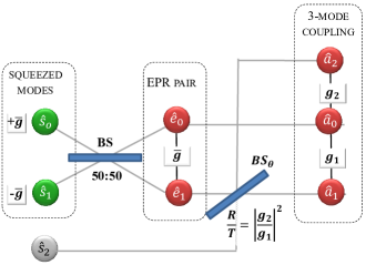
Figure 2: Bloch-Messiah decomposition of the tripartite entangled state generated by two concurrent parametric processes of strengths $g_{1}$ and $g_{2}$: $\hat{s}_{0}$ and $\hat{s}_{1}$ are squeezed modes, with opposite squeezing parameters $\pm\bar{g}z$, where $\bar{g}=\sqrt{|g_{1}|^{2}+|g_{2}|^{2}}$. $BS$ is a balanced beam-splitter, while $BS_{\theta}$ has a splitting ratio $R/T={|g_{2}|^{2}}/{|g_{1}|^{2}}$.

We observe that for the doubly-pumped crystal the effective squeezing parameter $\bar{r}=\bar{g}z\propto\sqrt{|\alpha_{1}|^{2}+\alpha_{2}|^{2}}$ is proportional to the square root of the total energy. Thus the level of squeezing coincides with what would be obtained by injecting in the same material a single pump with the same total energy. Conversely, for the single-pump NPC, $\bar{r}=\sqrt{2}\,g\propto\sqrt{2}|\alpha_{p}|$, i.e there is a net $\sqrt{2}$ increase of the amount of squeezing/gain in the 2D poled material, due to the coherent superposition of the two concurrent nonlinear processes.

Clearly, Fig. 2 can be read also in the inverse way: when a a member of an EPR pair with squeezing parameter $r=\bar{g}z$ is mixed with a vacuum input on a beam-splitter of transmission $T=\cos^{2}\theta$ , the result is the tripartite entangled state in the figure, obtained from the action of the momentum (17), with $g_{1}=\bar{g}\cos\theta$ and $g_{2}=\bar{g}\sin\theta$.

II.A Tripartite entanglement

We are now in conditions of applying the entanglement criteria outlined in sections I.B e I.C. Provided that squeezing is along the Y-quadrature for $\hat{s}_{0}$ while it is along the X-quadrature for $\hat{s}_{1}$, inversion of the matrix (19) permits to identify the nonlocal variables with sub-shot noise fluctuations. These are

$$\hat{\eta}({\mathbf{d}}) =\frac{1}{\sqrt{2}}\left(\hat{X}_{0}-\hat{X}_{1}\cos\theta-\hat{X}_{2}\sin\theta\right)=e^{-\bar{g}z}\hat{X}_{s_{1}}^{\mathrm{in}}$$ (23)

$$\hat{\eta}({\mathbf{d}}^{\prime}) =\frac{1}{\sqrt{2}}\left(\hat{Y}_{0}+\hat{Y}_{1}\cos\theta+\hat{Y}_{2}\sin\theta\right)=e^{-\bar{g}z}\hat{Y}_{s_{0}}^{\mathrm{in}}$$ (24)

where, according to the formalism developed in Sec.I, ${\mathbf{d}}=\frac{1}{\sqrt{2}}(1,-\cos\theta,-\sin\theta,0,0,0)^{\intercal}$, and ${\mathbf{d}}^{\prime}=\frac{1}{\sqrt{2}}(0,0,0,1,\cos\theta,\sin\theta)^{\intercal}$. The two variables commute $[\hat{\eta}({\mathbf{d}}),\hat{\eta}({\mathbf{d}}^{\prime})]=0$, so that there is no lower Heisenberg bound (7) to their variances. Indeed for vacuum input

$$\langle\delta\hat{\eta}^{2}({\mathbf{d}})\rangle=\langle\delta\hat{\eta}^{2}({\mathbf{d}}^{\prime})\rangle=e^{-2\bar{g}z}\to 0$$ (25)

for $\bar{g}z\gg 1$. Let us now check the bounds that must be obeyed by separable states. The bi-partitions of three modes are those corresponding to the 3 possible choices of a single mode with respect to the other two. Let us check them one by one, by applying the separability criterion of Eq.(14).

Separability of the shared mode $\hat{a}_{0}$.

The operation of partial transposition with respect to mode 0 corresponds in phase-space to the application of the mirroring matrix $\boldsymbol{\Gamma}_{0}=\mathrm{diag}\{1,1,1,-1,1,1\}$ that inverts the sign of $\hat{Y}_{0}$. Clearly, this has effect only on ${\mathbf{d}}^{\prime}$ $\to\Gamma_{0}{\mathbf{d}}^{\prime}=\frac{1}{\sqrt{2}}(0,0,0,-1,\cos\theta,\sin\theta)^{\intercal}$. Any state separable with respect to mode $0$ must respect the following bound

$$\langle\delta\hat{\eta}^{2}({\mathbf{d}})\rangle+\langle\delta\hat{\eta}^{2}({\mathbf{d}}^{\prime})\rangle\geq\left|[\hat{\eta}(\boldsymbol{\Gamma}_{0}{\mathbf{d}}^{\prime}),\hat{\eta}(\boldsymbol{\Gamma}_{0}{\mathbf{d}})]\right|=2$$ (26)

which is violated by our state for any finite amount of squeezing $\bar{g}z>0$. Therefore we conclude that mode 0 is never separable from the other two, as should be rather intuitive from the graph of the state in Fig.2.

Separability of mode $\hat{a}_{1}$.

Partial transposition with respect to mode 1 now transforms ${\mathbf{d}}^{\prime}\to\Gamma_{1}{\mathbf{d}}^{\prime}$ $=\frac{1}{\sqrt{2}}(0,0,0,1,-\cos\theta,\sin\theta)^{\intercal}$. The bound that must be respected by 1-separable states is

$$\langle\delta\hat{\eta}^{2}({\mathbf{d}})\rangle+\langle\delta\hat{\eta}^{2}({\mathbf{d}}^{\prime})\rangle \geq\left|\left[\hat{\eta}(\boldsymbol{\Gamma}_{1}{\mathbf{d}}^{\prime}),\hat{\eta}(\boldsymbol{\Gamma}_{1}{\mathbf{d}})\right]\right|$$ (27)

$$=\frac{1}{2}\left|\left[\hat{X}_{0}-\hat{X}_{1}\cos\theta-\hat{X}_{2}\sin\theta,\hat{Y}_{0}-\hat{Y}_{1}\cos\theta+\hat{Y}_{2}\sin\theta\right]\right|$$

$$=2\cos^{2}\theta$$

When applied to our tripartite state, using Eq.(25), a sufficient condition for inseparability of mode 1 is

$$\bar{g}z>\ln{\sqrt{1+\left|g_{2}/g_{1}\right|^{2}}}$$ (28)

which is shown in Fig.3a by the blue curve.

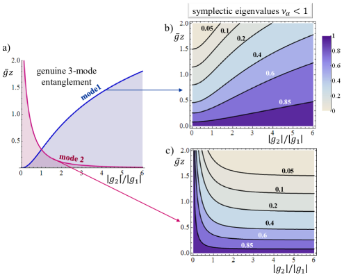
Figure 3: Entanglement of the 3-mode state (18). a) Sufficient criteria based on the violation of Heisenberg-like inequalities: mode 0 is never separable, while the entanglement of mode 1 and 2 is verified in the region above the blue and the red curve, respectively, according to (28) and (30). b) and c): Contour plots of the smallest symplectic eigenvalue $\nu_{-}^{(1)}$ and $\nu_{-}^{(2)}$ of the partial transpose with respect to mode 1 and 2, respectively, showing that actually entanglement is always present, unless trivially $g_{1}$ or $g_{2}$ vanish.

The condition becomes more and more demanding as $g_{1}\to 0$: when mode 1 is weakly coupled, more squeezing is required for verifying its entanglement.

Separability of mode $\hat{a}_{2}$.

In this case ${\mathbf{d}}^{\prime}$ $\to\Gamma_{2}{\mathbf{d}}^{\prime}=\frac{1}{\sqrt{2}}(0,0,0,1,\cos\theta,-\sin\theta)^{\intercal}$. States separable with respect to mode 2 must satisfy the inequality

$$\langle\delta\hat{\eta}^{2}({\mathbf{d}})\rangle+\langle\delta\hat{\eta}^{2}({\mathbf{d}}^{\prime})\rangle \geq\left|\left[\hat{\eta}(\boldsymbol{\Gamma}_{2}{\mathbf{d}}^{\prime}),\hat{\eta}(\boldsymbol{\Gamma}_{2}{\mathbf{d}})\right]\right|$$ (29)

$$=\frac{1}{2}\left|\left[\hat{X}_{0}-\hat{X}_{1}\cos\theta-\hat{X}_{2}\sin\theta,\hat{Y}_{0}+\hat{Y}_{1}\cos\theta-\hat{Y}_{2}\sin\theta\right]\right|$$

$$=2\sin^{2}\theta$$

As could be expected, the results for mode 2 are obtained from those of mode 1 by exchanging $\cos\theta\to\sin\theta$, or alternatively $g_{1}\to g_{2}$. For our tripartite state, using Eq.(25), a sufficient condition for inseparability of mode 2 is

$$\bar{g}z>\ln{\sqrt{1+\left|g_{1}/g_{2}\right|^{2}}}$$ (30)

which again become more and more demanding as $g_{2}\to 0$, i.e. as the coupling of mode 2 become weaker. The bound is shown in Fig.3 by the red curve labelled as ”mode 2”.

We notice that for $\cos\theta=\sin\theta$ (i.e. $g_{1}=g_{2}$) the bounds (27) and (29) coincides, and are always smaller than the bound for mode 0 in Eq.(26). Therefore, a sufficient condition for genuine tripartite entanglement which holds for any 3-mode state is that $\langle[\delta\hat{X}_{0}-(\delta\hat{X}_{1}+\delta\hat{X}_{2})/\sqrt{2}]^{2}\rangle+\langle[\delta\hat{Y}_{0}+(\delta\hat{Y}_{1}+\delta\hat{Y}_{2})/\sqrt{2}]^{2}\rangle<2$, and we retrieve the VanLoock-Furusawa criterion formulated in Eq.(21) of [29] (where a factor 4 in the numeric value of the bound arises from the different definitions of field quadratures). In the non-symmetric case, we find more in general that a sufficient criterion for genuine tripartite entanglement is

$$\langle[\delta\hat{X}_{0}-\delta\hat{X}_{1}\cos\theta-\delta\hat{X}_{2}\sin\theta]^{2}\rangle+\langle[\delta\hat{Y}_{0}+\delta\hat{Y}_{1}\cos\theta+\delta\hat{Y}_{2}\sin\theta]^{2}\rangle<4\min{\left[\cos^{2}\theta,\sin^{2}\theta\right]}$$ (31)

We stress that this is not the more general inequality for the variances of nonlocal observables, but it is one of the many which can be derived by systematic application of the Heisenberg-like inequalities in (14).

When applied to our tripartite state, the criterion is satisfied provided that

$$\bar{g}z>\begin{cases}\ln{\sqrt{1+\left|g_{2}/g_{1}\right|^{2}}}&\text{for }|g_{2}|\geq|g_{1}|\\ \ln{\sqrt{1+\left|g_{1}/g_{2}\right|^{2}}}&\text{for }|g_{2}|<|g_{1}|\end{cases}$$ (32)

Fig.3 summarizes the results for the tripartite entanglement of the state. Part a) of the figure shows the results of the test based on the violation of the Heisenberg-like inequalities (26, 27, 29) for the mirrored obervables: violation always occurs for mode $\hat{a}_{0}$, which is never unseparable, while the blue and red curves are the boundaries (28) and (30) above which the entanglement of $\hat{a}_{1}$ and $\hat{a}_{2}$ is verified . Therefore, the white zone above both curves guarantees the presence of a genuine tripartite entanglement, according to this test. We stress that these criteria are sufficient but not necessary, therefore the shaded regions below the curves may or may not be entangled.
Parts b) and c) of the figure, conversely, shows the result of the more powerful criterion directly based on the positivity of the partial transpose, specifically on the request in Eq. (11) that all the symplectic eigenvalues of $\boldsymbol{V}^{\mathsf{\,\scriptscriptstyle PT(A)}}$ are not below $1$ for A-separable states. For this low-dimensional case, the symplectic eigenvalues can be analytically calculated (Appendix A). For mode 1, the smallest symplectic eigenvalue of the partial transpose $\boldsymbol{V}^{\mathsf{\,\scriptscriptstyle PT(1)}}$ is

$$\nu_{-}^{(1)}=1+2[\cos\theta\sinh{(\bar{g}z)}]^{2}-\sqrt{\left[1+2[\cos\theta\sinh{(\bar{g}z)}]^{2}\right]^{2}-1}$$ (33)

which is always smaller than 1, unless $\cos\theta=0$ i.e. unless the coupling $g_{1}$ vanishes. The result for mode 2 can be obtained by switching $\cos\theta\to\sin\theta$: therefore also $\boldsymbol{V}^{\mathsf{\,\scriptscriptstyle PT(2)}}$ always has a symplectic eigenvalue $\nu_{-}^{(2)}<1$, a part from the limit case $\sin\theta=0$, when the coupling strength $g_{2}$ vanishes. Fig.3b) and 3c) plot contour lines of $\nu_{-}^{(1)}$ and $\nu_{-}^{(2)}$ in the parameter plane $(\frac{|g_{2}|}{|g_{1}|},\bar{g}z)$. It is important to remark that a symplectic eigenvalue $\nu_{\alpha}<1$ of the partial transpose not only certifies the entanglement, but also provides a measure of the bipartite entanglement, via e.g., the logarithmic negativity $\mathit{E}_{\mathcal{N}}=-\sum_{\nu_{\alpha}<1}\log_{2}\nu_{\alpha}$ [28], with smaller $\nu_{\alpha}$ corresponding to a larger amount of entanglement.

In conclusion, the state (18) always exhibits a genuine tripartite entanglement, revealed by the PPT criterion, which however becomes weaker in the limit of a strong unbalance between the two coupling strength $|g_{2}/g_{1}|\to 0$ or $|g_{2}/g_{1}|\to\infty$. In these limit situations, a larger amount of squeezing is necessary in order to detect the entanglement by means of the less powerful criteria based on violations of Heisenber-like bounds for the variances of nonlocal observables. This state is indeed a very good example of the fact that these criteria, although very useful and accessible, are indeed only sufficient to verify entanglement, and may fail to detect weakly entangled states.

III Doubly pumped bulk crystal, or single-pump NPC: 4-mode linear coupling.

An interesting feature of the 3-mode coupling generated by the hexagonally poled NPC is that several independent triplets of entangled modes coexist at any pair of conjugate wavelengths of the fluorescence radiation. As highlighted by Ref.[20], by tilting the direction of propagation of the pump field inside the medium, it is possible to reach special resonance conditions in which pairs of triplets, originally uncoupled, degenerate into a group of 4 entangled modes. This process takes place when the periodicity of the transverse phase modulation of the pump exactly matches that of the poling pattern, it involves the whole emission spectrum, and is accompanied by a sudden enhancement of the local gain [20]. Specifically, by considering the two triplets $\{\hat{a}_{0},\hat{a}_{1},\hat{a}_{2}\}$ and $\{\hat{a}_{0}^{\prime},\hat{a}_{1}^{\prime},\hat{a}_{2}^{\prime}\}$, at resonance the shared mode of each group superimpose to a coupled mode of the other, e.g. $\hat{a}_{0}\to\hat{a}_{1}^{\prime}$ and $\hat{a}_{0}^{\prime}\to\hat{a}_{1}$ . This gives rise to the 4-mode coupling shown in the graph (b2) of Fig.1, whose quantum properties were described as a Golden Ratio entanglement [17], because of the appearance of this particular irrational number. Recently, striking similar resonances have been demonstrated in a doubly pumped BBO crystal [21, 18]. Also in this second case the resonances are reached by tilting one of the pump modes inside the nonlinear medium, but their physical origin is quite different, because it involves the superposition of the Poynting vector of the pump carrier, representing the mean flux of the energy injected into the medium, with the direction of propagation of one pump mode [18]. As in the previous case, at resonance each two triplets of modes degenerate into a group of 4-modes, whose coupling is described by the scheme a2) of Fig.1. The only difference with the NPC case is the appearance of two distinct coupling strengths $g_{1}$ and $g_{2}$, controlled by the complex amplitudes $\alpha_{1},\alpha_{2}$ of the two pumps.

Let us focus on a specific group of 4-entangled modes $\{\hat{a}_{1},\hat{a}_{2},\hat{a}_{3},\hat{a}_{4}\}$. Their evolution equations along the sample can be found in [17] for the NPC and in [18] for the doubly pumped bulk crystal. They can be derived from a longitudinal momentum operator of the form

$$\hat{\cal P}={-i\hbar}\left(g_{1}\hat{a}_{1}^{\dagger}\hat{a}_{2}^{\dagger}+g_{2}\hat{a}_{2}^{\dagger}\hat{a}_{3}^{\dagger}+g_{2}\hat{a}_{4}^{\dagger}\hat{a}_{1}^{\dagger}-\text{h.c}\right),$$ (34)

where $\hat{a}_{1}$ and $\hat{a}_{2}$ are shared modes,characterized by two links in the graphs a2) and b2), while $\hat{a}_{3}$ and $\hat{a}_{4}$ are unshared modes, with a single link. We notice that these graphs correspond to a linear chain of nearest-neighbor interactions (we show them as open polygons to keep continuity with the previous works [18, 17]).

Refs.[17, 18] showed that the z-evolution of the four modes could be decomposed into two independent standard (i.e. 2-mode) parametric processes, mixed on an unbalanced beam-splitter. Based on these results, we can immediately derive the Bloch-Messiah decomposition of state. Let us first perform local phase rotations, inessential for entanglement: $(\hat{a}_{1},\hat{a}_{2})\to e^{\frac{i}{2}\arg(g_{1})}(\hat{a}_{1},\hat{a}_{2})$ and $(\hat{a}_{3},\hat{a}_{4})\to e^{i[\arg(g_{2})-\frac{1}{2}\arg(g_{1})]}(\hat{a}_{3},\hat{a}_{4})$, which eliminates from the problem the phases of $g_{1}$ and $g_{2}$ . This physically means that the phase(s) of the pump beam(s) are irrelevant for the entanglement of the state. Thus, as in the previous section, the parameter space is spanned by the two variables

$$x=\frac{|g_{2}|}{|g_{1}|},\quad \bar{r}=\sqrt{|g_{1}|^{2}+|g_{2}|^{2}}\,z$$ (35)

representing the unbalance between the two processes and the total squeezing/gain available for a medium of length $z$, respectively. Next we consider the transformation

$$\begin{pmatrix}\hat{a}_{1}\\ \hat{a}_{3}\\ \hat{a}_{2}\\ \hat{a}_{4}\end{pmatrix}=\frac{1}{\sqrt{2}}\begin{pmatrix}\cos\gamma&0&-\sin\gamma&0\\ 0&\cos\gamma&0&-\sin\gamma\\ \sin\gamma&0&\cos\gamma&0\\ 0&\sin\gamma&0&\cos\gamma\end{pmatrix}\begin{pmatrix}1&\phantom{,,}1&0&\phantom{,,}0\\ 1&-1&0&\phantom{,,}0\\ 0&\phantom{,,}0&1&\phantom{,,}1\\ 0&\phantom{,,}0&1&-1\end{pmatrix}\begin{pmatrix}\hat{s}_{1}\\ \hat{s}_{2}\\ \hat{s}_{3}\\ \hat{s}_{4}\end{pmatrix} =\mathbf{U}_{\textsc{B}}\begin{pmatrix}\hat{s}_{1}\\ \hat{s}_{2}\\ \hat{s}_{3}\\ \hat{s}_{4}\end{pmatrix}$$ (36)

where $\hat{s}_{1},\ldots\hat{s}_{4}$ are independent bosonic modes, and the angle $\gamma$ is defined by

$$\operatorname{tg}{\gamma}=\sqrt{\frac{\Lambda_{\delta}}{\Lambda_{\SS}}};\qquad \Lambda_{\sigma,\delta}(x)=\frac{\bar{g}}{\sqrt{x^{2}+1}}\frac{\sqrt{4x^{2}+1}\pm 1}{2}$$ (37)

Under this transformation the momentum operator in Eq.(34) becomes the product of 4 independent quadratic momenta,

$$\hat{\cal U}_{B}^{\dagger}\,\hat{\cal P}\,\hat{\cal U}_{B}=-i\hbar\left(\frac{\Lambda_{\sigma}}{2}\hat{s}_{1}^{\dagger}\hat{s}_{1}^{\dagger}-\frac{\Lambda_{\sigma}}{2}\hat{s}_{2}^{\dagger}\hat{s}_{2}^{\dagger}-\frac{\Lambda_{\delta}}{2}\hat{s}_{3}^{\dagger}\hat{s}_{3}^{\dagger}+\frac{\Lambda_{\delta}}{2}\hat{s}_{4}^{\dagger}\hat{s}_{4}^{\dagger}-h.c.\right)$$ (38)

where ${\mathcal{U}}_{B}$ is the generator of the transformation (36). As a result, the z-evolution of the 4-mode state decouples into the product of 4 single-mode squeeze operators $\hat{{\cal S}}_{j}(r)=\exp{(\frac{r}{2}\hat{s}_{j}^{\dagger}\hat{s}_{j}^{\dagger}-h.c.)}$, each acting on mode $j=1,\ldots 4$:

$$\hat{\cal U}_{B}^{\dagger}e^{\frac{i}{\hbar}\hat{\cal P}z}\hat{\cal U}_{B}=\hat{\cal S}_{1}(\Lambda_{\sigma}z)\otimes\hat{\cal S}_{2}(-\Lambda_{\sigma}z)\otimes\hat{\cal S}_{3}(-\Lambda_{\delta}z)\otimes\hat{\cal S}_{4}(\Lambda_{\delta}z).$$ (39)

where the squeeze parameters are given by Eq.(37).

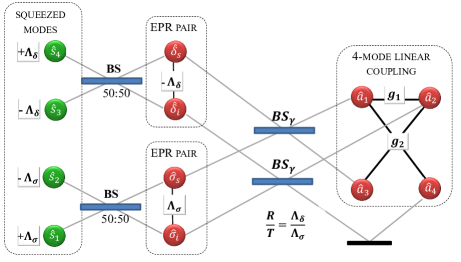
Figure 4: Bloch-Messiah decomposition of the 4-mode state (34), generated at resonance by a doubly pumped BBO or by a single-pump NPC. $\hat{s}_{1},..\hat{s}_{4}$ are independent squeezed modes, whose squeeze parameters $\pm\Lambda_{\sigma,\delta}z$ depend on $|g_{1}|$ and $|g_{2}|$ according to Eq.(37). $BS$ are balanced beam-splitters, while $BS_{\gamma}$ have $\frac{R}{T}=\operatorname{tg}^{2}\gamma=\frac{\Lambda_{\delta}}{\Lambda_{\sigma}}$. For the NPC, $\Lambda_{\sigma}=g\Phi$, $\Lambda_{\delta}=g/\Phi$, and $R/T=1/\Phi^{2}$, where $\Phi$ is the Golden Ratio.

For a vacuum input, the dynamics of the 4-mode state can be unfolded according to the scheme in Fig.4: here the 4 squeezed modes obtained from the action of the squeezers in Eq.(39) are first mixed on balanced beam-splitters to form two independent pairs of EPR modes, labelled as $\sigma_{s},\sigma_{i}$ and $\delta_{s},\delta_{i}$ -where ” s” and ”i” stand for signal and idler- with squeezing parameters $\Lambda_{\sigma}z$ and $-\Lambda_{\delta}z$, respectively. Next the EPR modes are pairwise mixed (signal with signal and idler with idler) on two identical beam splitters, whose splitting ratio is linked to the squeeze eigenvalues by

$$\frac{R}{T}=\frac{\Lambda_{\delta}}{\Lambda_{\sigma}},$$ (40)

Indeed, this is the condition which ensures that modes $\hat{a}_{3}$ and $\hat{a}_{4}$ are uncoupled, and that the graph of the coupling reduces to a linear chain.

We notice that for $x=1$ $\Lambda_{\SS}\to{\bar{g}\over\sqrt{2}}\Phi$ and $\Lambda_{\delta}\to{\bar{g}\over\sqrt{2}}{1\over\Phi}$, where $\Phi=\frac{1}{2}(1+\sqrt{5})$ is the Golden Ratio. Thus for the single-pump NPC, the squeeze parameters are $g\Phi$ and $g/\Phi$, and the ”Golden Ratio” squeezing or gain enhancement described in [20, 17] takes place. For the doubly-pumped BBO, one eigenvalue is always smaller than $\bar{g}$: $\Lambda_{\delta}/\bar{g}\in(0,1)$ but the other is always larger: ${\Lambda_{\sigma}}/\bar{g}\in(1,\frac{2}{\sqrt{3}})$, with the maximum value $2/\sqrt{3}=1.15..$ occurring when pump 2 is twice as intense as pump 1. Thus, at difference with the 3-mode case, the doubly-pumped scheme at resonance exhibits a true increase of the squeezing/gain level of certain modes, with respect to the use of a single-pump with the same energy .

III.A Quadripartite entanglement of the linear state.

As for the tripartite state, the 4-mode entanglement will be characterized both by using criteria based on variances of nonlocal observables [Eq.(14)], and by means of the symplectic eigenvalues of the partial transpose [Eq. (11)].

Inversion of the matrix (36) permits to identify the nonlocal variables with sub-shot noise fluctuations. Taking into account the sign of the squeezing parameters in Eq.(39), these are:

$$\hat{\eta}({\mathbf{d}}_{\SS}^{\prime}) =\frac{1}{\sqrt{2}}\left[\cos\gamma\left(\hat{Y}_{1}+\hat{Y}_{2}\right)+\sin\gamma\left(\hat{Y}_{3}+\hat{Y}_{4}\right)\right]=e^{-\Lambda_{\sigma}z}\hat{Y}_{s_{1}}^{\mathrm{in}}$$ (41a)

$$\hat{\eta}({\mathbf{d}}_{\SS}) =\frac{1}{\sqrt{2}}\left[\cos\gamma\left(\hat{X}_{1}-\hat{X}_{2}\right)+\sin\gamma\left(\hat{X}_{3}-\hat{X}_{4}\right)\right]=e^{-\Lambda_{\sigma}z}\hat{X}_{s_{2}}^{\mathrm{in}}$$ (41b)

$$\hat{\eta}({\mathbf{d}}_{\delta}) =\frac{1}{\sqrt{2}}\left[-\sin\gamma\left(\hat{X}_{1}+\hat{X}_{2}\right)+\cos\gamma\left(\hat{X}_{3}+\hat{X}_{4}\right)\right]=e^{-\Lambda_{\delta}z}\hat{X}_{s_{3}}^{\mathrm{in}}$$ (41c)

$$\hat{\eta}({\mathbf{d}}_{\delta}^{\prime}) =\frac{1}{\sqrt{2}}\left[-\sin\gamma\left(\hat{Y}_{1}-\hat{Y}_{2}\right)+\cos\gamma\left(\hat{Y}_{3}-\hat{Y}_{4}\right)\right]=e^{-\Lambda_{\delta}z}\hat{Y}_{s_{4}}^{\mathrm{in}}$$ (41d)

By construction, the variables commute pairwise $\left[\hat{\eta}({\mathbf{d}}_{\alpha}),\hat{\eta}({\mathbf{d}}_{\beta}^{\prime})\right]=0$ and their variances asymptotically vanish in the limit of large squeezing $\bar{g}z>>1$

$$\left\langle\delta\hat{\eta}^{2}({\mathbf{d}}_{\alpha})\right\rangle=\left\langle\delta\hat{\eta}^{2}({\mathbf{d}}_{\alpha}^{\prime})\right\rangle=e^{-2\Lambda_{\alpha}z},\qquad(\alpha=\sigma,\delta)$$ (42)

Conversely, if we consider states that are separable with respect to a given partition $\{A\}\times\{B\}$ of the set of four modes, the variances of the observables (41) are constrained by the four bounds that arise from the nonzero commutators of the mirrored variables. Precisely, by using Eq. (14), these bounds are

$$\left\langle\delta\hat{\eta}^{2}({\mathbf{d}}_{\alpha})\right\rangle+\left\langle\delta\hat{\eta}^{2}({\mathbf{d}}_{\alpha}^{\prime})\right\rangle \geq\left|\left[\eta(\boldsymbol{\Gamma}_{A}{\mathbf{d}}_{\alpha}),\eta(\boldsymbol{\Gamma}_{A}{\mathbf{d}}_{\alpha}^{\prime})\right]\right|\qquad(\alpha=\sigma,\delta)$$ (43a)

$$2\sqrt{\left\langle\delta\hat{\eta}^{2}({\mathbf{d}}_{\alpha})\right\rangle\,\langle\delta\hat{\eta}^{2}({\mathbf{d}}_{\beta}^{\prime})\rangle} \geq\left|\left[\eta(\boldsymbol{\Gamma}_{A}{\mathbf{d}}_{\alpha}),\eta(\boldsymbol{\Gamma}_{A}{\mathbf{d}}_{\beta}^{\prime})\right]\right|\qquad(\alpha\neq\beta=\sigma,\delta)$$ (43b)

where $\boldsymbol{\Gamma}_{A}$ is the mirror matrix defined by Eq. (8). Notice that for $\alpha\neq\beta$ [Eq. (43b)] we directly wrote the criterion for the product of variances because in this case it is more stringent than the one for the sum. Violation of any of these bounds is sufficient to verify that the state is not A-separable.

For each of the possible partitions of the system, we checked the four constraints, and we chose among them the one that is violated first in terms of the total gain (see table 4 in Appendix B). The seven distinct partitions of four modes are listed below:

$P_{1}$	$P_{2}$	$P_{3}$	$P_{4}$	$P_{12}$	$P_{13}$	$P_{14}$
$\{1\}\times\{2,3,4\}$	$\{2\}\times\{1,3,4\}$	$\{3\}\times\{1,2,4\}$	$\{4\}\times\{1,2,3\}$	$\{1,2\}\times\{3,4\}$	$\{1,3\}\times\{2,4\}$	$\{1,4\}\times\{2,3\}$

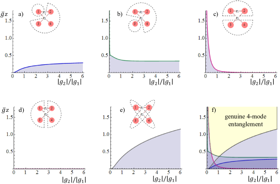
Figure 5: Entanglement of the 4-mode linear state (34), according to sufficient criteria based on the violation of the Heisenberg-like inequalities (43). Plots a) to e) are the results for partitions $P_{1}$, $P_{3}$, $P_{12}$, $P_{13}$ and $P_{14}$, respectively, where inseparability is guaranteed in the region above the curve. The plots for $P_{2}$ and $P_{4}$ are identical to those for $P_{1}$ and $P_{3}$, respectively. f) summarizes all the bounds, with a genuine 4-party entanglement being verified in the yellow region above all curves.

The panels from a) to e) of Fig.5 show the results obtained for each bipartition. The curves plot the lowest one of the constraints (43), so that in the white region above each curve all the Heisenberg-like inequalities (43) are violated, which guarantees that the state is inseparable with respect to the given partition. We remind that the criterion is only sufficient, so that the shaded regions below each curve may or may not be entangled. For reasons of symmetry, the results for $P_{2}$ and $P_{4}$ are identical to those for $P_{1}$ and $P_{3}$, respectively, and therefore are not shown. Panel f) summarizes all the bounds, where the yellow region above all curves guarantees the presence of a genuine quadripartite entanglement, according to this test. Notice that violation always occur for partition $P_{13}$ [panel d)], implying that for any finite gain $\bar{g}z\neq 0$ the state is never fully separable. This is a straightforward consequence of the existence in the subspace $\{\hat{a}_{1},\hat{a}_{3}\}$ of linear combinations of modes, namely the EPR signal modes $\sigma_{s}$ and $\delta_{s}$ in figure 4, that are maximally entangled to their EPR partners $\sigma_{i}$ and $\delta_{i}$ living in the complementary subspace $\{\hat{a}_{2},\hat{a}_{4}\}$.

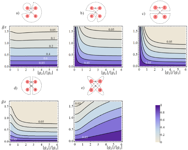
Figure 6: Entanglement of the 4-mode linear state (34), according to the PPT criterion. a) to e) are contour plots of the symplectic eigenvalues $\nu_{\alpha}<1$ of $V^{\mathsf{\,\scriptscriptstyle PT(A)}}$ listed in Table 2, for each partition. For $P_{1}$, $P_{3}$ and $P_{14}$ there is a single eigenvalue $\nu_{\alpha}<1$, shown in a), b) and e) ( the results for $P_{2}$ and $P_{4}$ are identical to those for $P_{1}$and $P_{3}$, respectively, and are not shown), For $P_{12}$ and $P_{13}$, panels c) and d) show the product of the two eigenvalues below 1.

Fig.6 shows instead the results of the more powerful test based on the PPT criterion, namely on the request [Eq. (11)] that for A-separable states all the symplectic eigenvalues of $\boldsymbol{V}^{\mathsf{\,\scriptscriptstyle PT(A)}}$ satisfy $\nu_{\alpha}\geq 1$. For each of the seven bipartitions, the symplectic spectra have been analytically calculated, and are reported in table 2 of Appendix A. Fig.6 shows contour plots, in the parameter plane $(|g_{2}/g_{1}|,\bar{g}z)$, of the product $\prod_{\nu_{\alpha}<1}\nu_{\alpha}$. We remind that this quantity provides a quantitative assessment of the bipartite entanglement, via the logarithmic negativity $\mathit{E}_{\mathcal{N}}=-\log_{2}\left(\prod_{\nu_{\alpha}<1}\nu_{\alpha}\right)$ [28].
As already noticed for the 3-mode state, the PPT criterion reveals the presence of entanglement in regions of the parameter space where the Heisenberg-like criteria (43) fail to detect it. Actually, according to the results in Fig.6, the four-mode linear state exhibits a genuine 4-party entanglement for any finite value of the gain $\bar{g}z$, unless trivially one of the two couplings vanishes, $g_{1}=0$ or $g_{2}=0$ In particular, for the single-pump NPC, where $g_{2}=g_{1}=\sqrt{2}\bar{g}$, the 4-mode entanglement is always a genuine one.
Indeed the analysis of the symplectic spectra provides a quantitative assessment of what could be intuitively expected for a linear chain of nearest neighbor interactions. Assuming a given amount of the total gain $\bar{g}z>0$, the shared modes 1 and 2, characterized by two links of strength $g_{1}$ and $g_{2}$ with the other modes, are never separable [panel a)], and their level of entanglement remains fairly constant with the ratio $|g_{2}/g_{1}|$. Conversely, the entanglement of modes 3 and 4, which have the single link $g_{2}$, is weaker and vanishes for $g_{2}\to 0$ [panel b)]. Concerning the 2 $\times$ 2 bipartitions, we notice that $P_{12}$ [panel c)] has a double link of strength $g_{2}$: therefore, it may become separable for $g_{2}=0$, but has a quite high level of entanglement when $|g_{2}|>|g_{1}|$. In comparison, $P_{14}$ [panel e)], which becomes separable for $g_{1}\to 0$, has a weaker entanglement because it has a single link. The ”signal-idler” partition $P_{13}$ [panel d)] is clearly the most entangled one: it is never separable, because its three links of different strengths cannot simultaneously vanish for $\bar{g}z>0$. In this case, the symplectic eigenvalues $\nu_{\alpha}<1$ of the partial transpose have the particularly simple expressions $e^{-2\Lambda_{\delta}z}$ and $e^{-2\Lambda_{\delta}z}$ [table 2], where $\Lambda_{\sigma}z$ and $\Lambda_{\delta}z$ are the squeeze parameters of the Bloch-Messiah decomposition of the state, given by Eq. (37). Using this equation, after some simple calculations, the logarithmic negativity turns up $\mathit{E}_{\mathcal{N}}=\frac{2}{\ln 2}\sqrt{4|g_{2}|^{2}+|g_{1}|^{2}}$ . Thus, for $g_{2}=0$ $\mathit{E}_{\mathcal{N}}\to\frac{2}{\ln 2}|g_{1}|z$, which is the logarithmic negativity of a single EPR state with gain $|g_{1}|z$ , while for $g_{1}=0$, $\mathit{E}_{\mathcal{N}}\to\frac{4}{\ln 2}|g_{2}|z$, corresponding to the entanglement of two independent EPR states.

IV Doubly pumped NPC: 4-mode square coupling

The last example that we consider is that of doubly pumped NPC, schematically shown by Fig.1c: here the intensity pattern created by the interference of the two pump modes superimposes to the static pattern of the periodic poling. The four possible combinations of the pump modes with the grating vectors $\vec{G}_{1}$ and $\vec{G}_{2}$ drive four concurrent processes which create four families of intersecting cones [19, 22]. A specially important configuration is reached at spatial resonance, when the periodicity of the pump pattern matches that of the poling pattern, and two of the four processes degenerate into a single one, whose parametric gain is controlled by the coherent sum of the two pump amplitudes $\ |\alpha_{1}+\alpha_{2}|$ [19, 22]. This gives rise to the four-mode coupling shown in Fig.1c2) in proper groups of spatio-temporal light modes. Remarkably, this coupling is topologically different from the one of the single-pump NPC, because it is a closed square chain of nearest-neighbor interactions.

As detailed in Ref.[19], the generator of the $z-$evolution along the sample of each quadruplet of coupled modes is the longitudinal momentum

$$\hat{\cal P}={-i\hbar}\left(g_{1}\hat{a}_{1}^{\dagger}\hat{a}_{2}^{\dagger}+(g_{1}+g_{2})\hat{a}_{2}^{\dagger}\hat{a}_{3}^{\dagger}+g_{2}\hat{a}_{3}^{\dagger}\hat{a}_{4}^{\dagger}+(g_{1}+g_{2})\hat{a}_{4}^{\dagger}\hat{a}_{1}^{\dagger}-\text{h.c}\right).$$ (44)

We notice that in this case all modes are shared between two of the three processes, and are characterized by two links in the graph of Fig. 7. We also notice that the central links have strengths $g_{1}+g_{2}$ controlled by the phases of $g_{1}$ and $g_{2}$, i.e. by the phases of the pump modes, which represents the specific feature of this configuration, absent in the case of the doubly pumped bulk crystal where the phases were irrelevant.

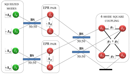
Figure 7: Bloch-Messiah decomposition of the 4-mode state (44), generated at resonance by a NPCpumped by two pumps of equal intensity $|g_{1}|=|g_{2}|$. Modes $\hat{s}_{1},..\hat{s}_{4}$ have squeeze parameters $\pm\Lambda_{\sigma,\delta}z$ which depend on the pump phase-difference $\phi_{-}$ as described by Eq.(48). $BS$ are balanced beam-splitters.

In order to emphasize this feature (and also for reasons for brevity), in the following we limit our analysis to the symmetric case, in which the pumps have equal intensities and

$$|g_{1}|=|g_{2}|$$ (45)

By performing the local phase rotations $(\hat{a}_{1},\hat{a}_{2})\to e^{\frac{i}{2}\arg(g_{1})}(\hat{a}_{1},\hat{a}_{2})$ and $(\hat{a}_{3},\hat{a}_{4})\to-e^{\frac{i}{2}\arg(g_{2})]}(\hat{a}_{3},\hat{a}_{4})$, the momentum operator reduces to $\hat{\cal P}={-i\hbar}\frac{\bar{g}}{\sqrt{2}}\left[\hat{a}_{1}^{\dagger}\hat{a}_{2}^{\dagger}+\hat{a}_{3}^{\dagger}\hat{a}_{4}^{\dagger}+2\cos\phi_{-}(\hat{a}_{2}^{\dagger}\hat{a}_{3}^{\dagger}+\hat{a}_{4}^{\dagger}\hat{a}_{1}^{\dagger})-\text{h.c}\right]$. The parameter space is spanned by the two variables

$$\phi_{-}=\frac{\arg(g_{1})-\arg(g_{2})}{2}\quad \bar{r}=\sqrt{|g_{1}|^{2}+|g_{2}|^{2}}\,z$$ (46)

representing the phase shift between the two processes (physically, $\phi_{-}$ is the offset between the transverse modulations of the pump and of the poling pattern [19]) and the total squeezing/gain available for a medium of length $z$.

The Bloch-Messiah decomposition of state is shown in Fig.7; it is obtained by means of the transformation

$$\begin{pmatrix}\hat{a}_{1}\\ \hat{a}_{3}\\ \hat{a}_{2}\\ \hat{a}_{4}\end{pmatrix}=\frac{1}{2}\begin{pmatrix}1&\phantom{,,}1&\phantom{,,}1&\phantom{,,}1\\ 1&-1&1&-1\\ 1&\phantom{,,}1&-1&-1\\ 1&-1&-1&1\end{pmatrix}\begin{pmatrix}\hat{s}_{1}\\ \hat{s}_{2}\\ \hat{s}_{3}\\ \hat{s}_{4}\end{pmatrix} =\mathbf{U}_{\textsc{B}}\begin{pmatrix}\hat{s}_{1}\\ \hat{s}_{2}\\ \hat{s}_{3}\\ \hat{s}_{4}\end{pmatrix}$$ (47)

where the squeezed modes $\hat{s}_{1},\hat{s}_{2},\hat{s}_{3},\hat{s}_{4}$ have squeeze parameters $+\Lambda_{\sigma}z,-\Lambda_{\sigma}z,-\Lambda_{\delta}z,+\Lambda_{\delta}z$ in order, with

$$\Lambda_{\sigma,\delta}=\frac{\bar{g}}{\sqrt{2}}\left(2\cos\phi_{-}\pm 1\right)=|g_{1}+g_{2}|\pm|g_{1}|$$ (48)

We notice that the decomposition is very similar to the one in Fig.4, but the condition (40) is released, with the $BS_{\gamma}$ replaced by balanced beam-splitters, having $R/T=\operatorname{tg}^{2}\gamma=1$.

IV.A Quadripartite entanglement of the square state

For the state generated by the square coupling (44) we omit the long but simple analysis based on the variances of nonlocal observables, which can be performed along the guidelines of the previous sections, by inverting the transformation (47) (some caution should be taken with the sign of $\Lambda_{\delta}$). As in the other examples, this kind of analysis does not actually add anything to the results based on the symplectic eigenvalues of the partial transpose matrix $\boldsymbol{V}^{\mathsf{\,\scriptscriptstyle PT(A)}}$, which for this simple state can be analytically performed and are presented in Fig.8.

Before discussing these results, let us consider the following points: According to our definitions, $\Lambda_{\delta}$ in Eq.(48) is positive for $\phi_{-}<\frac{\pi}{3}$ and negative for $\phi_{-}>\frac{\pi}{3}$. The point $\phi_{-}=\frac{\pi}{3}$ ($\!\mod\pi$) at which $\Lambda_{\delta}=0$ and modes $\hat{s}_{3}$ and $\hat{s}_{4}$ are not squeezed is characterized by the fact that all the intermodal links have the same strength: $|g_{1}+g_{2}|=|g_{1}|=|g_{2}|$. At this point, the 4-mode state corresponds to a balanced mixture of an EPR state with a vacuum or coherent state, as discussed in [19]. The other important point is $\phi_{-}=\frac{\pi}{2}$ at which $g_{1}+g_{2}=0$, and the two central links vanish, so that the 4-mode coupling degenerates into the product of two independent 2-mode couplings. At this point $\Lambda_{\delta}=-\Lambda_{\sigma}$, and, according to the Bloch-Messiah decomposition in Fig. 7, the state is the mixture of two identical EPR states on a balanced beam-splitter, which again results into two independent EPR pairs. Correspondingly, we expect that the quadripartite entanglement of the state ceases to be a genuine one.

These considerations are well reflected by the analysis of the entanglement based on the PPT criterion. Table 3 reports our results for the symplectic spectrum of the partial transpose matrix $\boldsymbol{V}^{\mathsf{\,\scriptscriptstyle PT(A)}}$, and shows the conditions for having symplectic eigenvalues $\nu_{\alpha}<1$ which guarantee the inseparability with respect to each given partition. Fig.8 shows countour plots of the product $\prod_{\nu_{\alpha}<1}\nu_{\alpha}$ in the parameter plane $(\phi_{-},\bar{g}z)$ for each partition of the system. Panel a) shows the results for the 1-mode partitions, which in this case are all identical, because of the symmetry of state. These partitions are never separable, because each mode has one link of strength $|g_{1}|=|g_{2}|$ that never vanishes, while the strength of the other $|g_{1}+g_{2}|=2|g_{1}|\cos\phi_{-}$ decreases from $\phi_{-}=0$ to $\phi_{-}={\pi\over 2}$, and this behavior is reflected by the entanglement of the partition. $P_{12}=\{1,2\}\times\{3,4\}$ is the only partition which becomes separable at $\phi_{-}={\pi\over 2}$, where its double link $g_{1}+g_{2}$ vanishes. The signal-idler partition $P_{13}$ is always entangled, and so does the partition $\{1,4\}\times\{2,3\}$: in this last case the amount of entanglement remains constant with the phase-difference $\phi_{-}$, because the strengths of its two links are $|g_{1}|=|g_{2}|$.

h

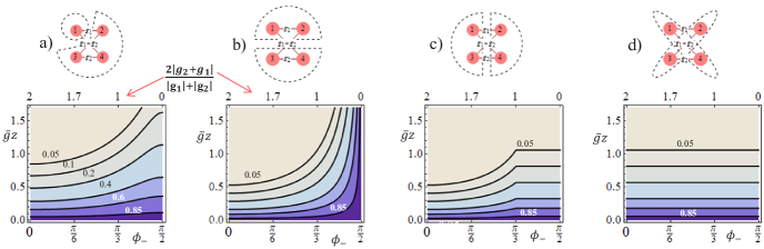
Figure 8: Entanglement of the 4-mode square state (44), according to the PPT criterion. a) to e) are contour plots of the product of the symplectic eigenvalues $\nu_{\alpha}\leq 1$ of $V^{\mathsf{\,\scriptscriptstyle PT(A)}}$ listed in Table 3, for each partition of the system. a) shows the results for the 1-mode partitions $P_{j}$, which are all are all identical; b),c) and d) are the results for the remaining partitions. The quadripartite entanglement is always genuine, except at the point $\phi_{-}={\pi\over 2}$, where $g_{1}+g_{2}=0$ and $P_{12}$ in b) becomes separable.

V Discussion and Conclusions

There are two kind of conclusions which can be drawn from this analysis.

From the point of view of physics, it has been shown that a genuine multipartite entanglement among separate spatial modes of the electromagnetic field can be generated by spatially engineering the effective nonlinearity of parametric sources. In this work, this is achieved by a simple transverse modulation of the pump beam driving the process and/or of the nonlinear response in a NPC. The quantum states generated in this way are rather simple, since the entanglement is limited to sets of three or four modes; as such, they cannot compete at the present stage of analysis with the multipartite states generated by more powerful schemes based on on tailoring the spectral entanglement of frequency combs [12, 13, 14, 15]. However more complex setting may be envisaged, involving more spatial modes of the pump beam or more reciprocal vectors of the nonlinear pattern of the NPC. For example, one may think of driving a parametric process by means of N plane-wave pumps, whose wavevectors are symmetrically tilted over a conical surface, similarly to the scheme proposed in Ref. [35]. Preliminary investigations have shown [36] that there exist realistic configurations (in terms of the choice of the material, of the type of interaction, of the frequencies involved etc.) in which N modes of the down-converted radiations may become coupled one to each other, according to a closed chain of nearest neighbor interactions, realizing thus a higher dimensional version of the square 4-mode entanglement described in Sec.IV. In the same setup, by slightly changing the parameters it can be also achieved a situation in which there is a single central mode of the down-converted light coupled to each of N spatially separated modes [36], thus realizing the multipartite entanglement analysed in [35].
It should be also noticed that even in the simpler setup considered in this paper (N=2, or equivalently, two reciprocal vectors of the nonlinear grating) there are actually infinite sets of triplets (or quadruplets) of entangled modes which coexist independently in the same beam. These are distinguished by their spatial coordinates in one transverse direction, say $y$, as e.g. shown by Figs. 6 and 7 in [17]. Strategies for entangling independent groups of modes in a higher dimensional state could be envisaged; for example by employing in the spatial domain techniques analogue to those used in the temporal domain to generate the XEPR state in Ref.[10], with the temporal delay being replaced by a spatial shift.
We hope that the proof-of-principle analysis performed in this work may stimulate experimental work in this sense.

The second conclusion is more on the formal side and concerns the effectiveness of the various strategies for detecting entanglement. We formulated general bounds [Eq. (14)] which must be respected by states that are separable with respect to a given partition of the system. As previously mentioned, these inequalities are not fundamentally new compared to similar ones that can be found in the existing literature [29, 31, 32], but have the merit of a very general and expressive form, in which the variances of nonlocal observables are bounded by the commutators of the corresponding ”mirrored” observables. Moreover, for a given Gaussian state, we suggested a simple method for identifying the nonlocal observables that are most likely to certify its entanglement, based on its Bloch-Messiah decomposition. The states examined in this work, thanks to their relative simplicity, gave us the possibility of verifying to what extend these criteria are efficient in detecting the entanglement. By performing analytical calculations of the various symplectric spectra involved, we have shown that, although weaker than the PPT criteria which require the whole covariance matrix, the more experimentally accessible criteria based on the Heisenberg-like inequalities (14) capture the essential structure of the entanglement of the state (but, clearly, they are unable to give any quantitative assessment).

Appendix A Symplectic spectra

A.A Williamson normal form and symplectic eigenvalues

According to a theorem due to Williamson [37], any real, positive-definite, symmetric $2N\times 2N$ matrix can be brought to a diagonal form by means of a linear basis change that preserves the symplectic form $\boldsymbol{\Omega}$. When applied to the covariance matrix, it implies that any covariance matrix can be written as $\boldsymbol{V}=\boldsymbol{S}\boldsymbol{V}^{\mathrm{in}}\boldsymbol{S}^{\intercal}$, where $\boldsymbol{V}^{\mathrm{in}}=\mathrm{diag}\{\nu_{1},\nu_{2}\ldots\nu_{N},\nu_{1},\nu_{2}\ldots\nu_{N}\}$, and $\boldsymbol{S}$ is a symplectic transformation , i.e. a 2Nx2N matrix that preserves the fundamental commutation relation $\boldsymbol{S}^{\intercal}\boldsymbol{\Omega}\boldsymbol{S}=\boldsymbol{\Omega}$. The set of N positive numbers $\boldsymbol{\nu}=\{\nu_{1},\nu_{2}\ldots\nu_{N}\}$ is called the symplectic spectrum of $\boldsymbol{V}$, and can be obtained by calculating the eigenvalues of $i\boldsymbol{\Omega}\boldsymbol{V}$ which are $\pm\nu_{1},\pm\nu_{2}\ldots\pm\nu_{N}$. Then, the inequality (4) implies that for a legitimate covariance matrix $\nu_{\alpha}\geq 1$ , $\forall\alpha=1,\ldots,N$, which physically corresponds to $\boldsymbol{V}^{\mathrm{in}}$ being the covariance matrix of N independent thermal states. For pure Gaussian states, $\nu_{\alpha}=1$ , $\forall\alpha=1,\ldots,N$.

Considering a partition $\{A\}\times\{B\}$ of the system, the partial transpose matrix $\boldsymbol{V}^{\mathsf{\,\scriptscriptstyle PT(A)}}$ is still real, positive definite and symmetric. Therefore the Williamson theorem can applied to it, and the symplectic spectrum calculated from the eigenvalues of $i\boldsymbol{\Omega}\boldsymbol{V}^{\mathsf{\,\scriptscriptstyle PT(A)}}$. In this case, however, nothing ensures that $\nu_{\alpha}\geq 1$: only for A-separable states, $\boldsymbol{V}^{\mathsf{\,\scriptscriptstyle PT(A)}}$ is a legitimate covariance matrix, and its symplectic spectrum must satisfy $\nu_{\alpha}\geq 1$ , $\forall\alpha=1,\ldots,N$. Conversely, the appearance of an eigenvalue $\nu_{\alpha}<1$ in the symplectic spectrum of the partial transpose is sufficient to demonstrate that the state is not A-separable.

A.B Calculation of the symplectic spectra of the partial transpose

For each state considered in the main text, its Bloch Messiah reduction was exploited in order to calculate the covariance matrix $\boldsymbol{V}$ associated with the state, following the procedure described in Sec.I.C, see in particular equation (16). For each partition $\{A\}$$\times$$\{B\}$ of the system, the partial transpose matrix was then calculated as $\boldsymbol{V}^{\mathsf{\,\scriptscriptstyle PT(A)}}=\boldsymbol{\Gamma}_{A}\boldsymbol{V}\boldsymbol{\Gamma}_{A}$, where $\boldsymbol{\Gamma}_{A}$ is the mirror transformation (8). Finally, the characteristic polynomial associated to the matrix $i\boldsymbol{\Omega}\boldsymbol{V}^{\mathsf{\,\scriptscriptstyle PT(A)}}$ was analysed, and its eigenvalues calculated with the help of Wolfran Mathematica [38].
Results for the 3-mode state (18) are shown in table 1. The results for the 4-mode linear state (34) are provided by table 2, while figure 9 plots the corresponding eigenvalues $\nu_{\alpha}<1$ (or $\prod_{\nu_{\alpha}<1}\,\nu_{\alpha}$ when there is more then one) as a function of the total gain $\bar{g}z$. Finally, table 3 lists the symplectric spectra for the four-mode square state (44).

Partition	Symplectic spectrum of $V^{\mathsf{\,\scriptscriptstyle PT(A)}}$			$\nu_{\alpha}<1$
A	spectrum	eigenvalues
$\{0\}$	$\left(\begin{smallmatrix}e^{-2\bar{g}z},&1,&e^{2\bar{g}z}\end{smallmatrix}\right)$			$e^{-2\bar{g}z}$   none
$\{1\}$	$\left(\begin{smallmatrix}\nu_{-},&1,&\nu_{+}\end{smallmatrix}\right)$	$\nu_{\pm}=b\pm\sqrt{b^{2}-1}$	$\bullet$ $b=1+2[\cos\theta\sinh{(\bar{g}z)}]^{2}$	$\nu_{-}$   $g_{1}\neq 0$
$\{2\}$	$\left(\begin{smallmatrix}\nu_{-},&1,&\nu_{+}\end{smallmatrix}\right)$	$\nu_{\pm}=b\pm\sqrt{b^{2}-1}$	$\bullet$ $b=1+2[\sin\theta\sinh{(\bar{g}z)}]^{2}$	$\nu_{-}$   $g_{2}\neq 0$

Table 1: Three-mode coupling(18): symplectic spectrum of the partial transpose matrix. The first column indicates the partition, via the Alice set A; the second column describes the symplectic spectrum of $V^{\mathsf{\,\scriptscriptstyle PT(A)}}$, where $\theta$ and $\bar{g}$ are the parameters of the Bloch-Messiah decomposition in Eqs.(20) and (22). The last column gives the smallest eigenvalue and the conditions for $\nu_{\alpha}<1$ ensuring inseparability.

Partition	Symplectic spectrum of $V^{\mathsf{\,\scriptscriptstyle PT(A)}}$		$\nu_{\alpha}\leq 1$
A	Spectrum	Eigenvalues
$\{1\}$ or $\{2\}$	$\left(\begin{smallmatrix}\nu_{-},&1,&1,&\nu_{+}\end{smallmatrix}\right)$	$\nu_{\pm}=\sqrt{b\pm\sqrt{b^{2}-1}}$   $\bullet$ $b=2\left[\cosh(2r_{\sigma})\cos^{2}{\gamma}+\cosh(2r_{\delta})\sin^{2}\gamma\right]^{2}-1$	$\nu_{-}$	none
$\{3\}$ or $\{4\}$	$\left(\begin{smallmatrix}\nu_{-},&1,&1,&\nu_{+}\end{smallmatrix}\right)$	$\nu_{\pm}=\sqrt{b\pm\sqrt{b^{2}-1}}$   $\bullet$ $b=2\left[\cosh(2r_{\sigma})\sin^{2}{\gamma}+\cosh(2r_{\delta})\cos^{2}\gamma\right]^{2}-1$	$\nu_{-}$	$g_{2}\neq 0$
$\{1,2\}$	$\left(\begin{smallmatrix}\nu_{-},&\nu_{-},&\nu_{+},&\nu_{+}\end{smallmatrix}\right)$	$\nu_{\pm}=\sqrt{1+a^{2}}\pm a$   $\bullet$ $a=\sin(2\gamma)\sinh(r_{\delta}+r_{\sigma})$	$\nu_{-}$ $\nu_{-}$	$g_{2}\neq 0$
$\{1,3\}$	$(\begin{smallmatrix}e^{-2r_{\sigma}},&e^{-2r_{\delta}},&e^{2r_{\delta}},&e^{2r_{\sigma}}\end{smallmatrix})$		$e^{-2r_{\sigma}}$ $e^{-2r_{\delta}}$	none
$\{1,4\}$	$\left(\begin{smallmatrix}\nu_{-},&\nu_{+},&\mu_{-},&\mu_{+}\end{smallmatrix}\right)$	$\nu_{\pm}=e^{-c}\sqrt{p\pm\sqrt{p^{2}-1}}$     $\bullet$ $c=r_{\sigma}-r_{\delta}\geq 0$	$\nu_{-}$	$g_{1}\neq 0$
		$\mu_{\pm}=\sqrt{pe^{2c}\pm e^{-2c}\sqrt{p^{2}-1}}$   $\bullet$ $p=1+2[\cos(2\gamma)\sinh(r_{\delta}+r_{\sigma})]^{2}$

Table 2: Four-mode linear coupling(34): symplectic spectrum of the partial transpose. The first column indicates the bipartition, via the Alice set A; the second column describes the symplectic spectrum of $V^{\mathsf{\,\scriptscriptstyle PT(A)}}$, where $\gamma$ and $r_{\sigma,\delta}=\Lambda_{\sigma,\delta}z$ are the parameters of the Bloch-Messiah decomposition of the state in Eq.(37). The last column lists the eigenvalues $\nu_{\alpha}\leq 1$, and the conditions that guarantee inseparability through $\nu_{\alpha}<1$.

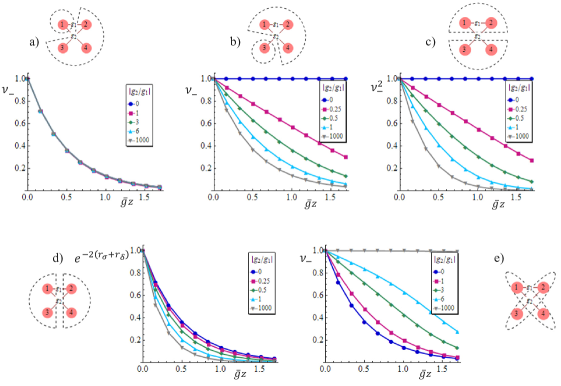
Figure 9: Four-mode linear coupling: symplectic eigenvalues $\nu_{\alpha}\leq 1$ of $V^{\mathsf{\,\scriptscriptstyle PT(A)}}$ listed in table 2. a) to e) show $\prod_{\nu_{\alpha}<1}\nu_{\alpha}$ for each partition. The plots for partitions $P_{2}$ and $P_{4}$ are identical to those for $P_{1}$and $P_{3}$ in panels a) and b), respectively.

Partition	Symplectic spectrum of $V^{\mathsf{\,\scriptscriptstyle PT(A)}}$		$\nu_{\alpha}<1$
A	Spectrum	Eigenvalues
$\{j=1,..4\}$	$\left(\begin{smallmatrix}\nu_{-},&1,&1,&\nu_{+}\end{smallmatrix}\right)$	$\nu_{\pm}=\sqrt{b\pm\sqrt{b^{2}-1}}$   $\bullet$ $b=\frac{1}{2}\left[\cosh(2r_{\sigma})+\cosh(2r_{\delta})\right]^{2}-1$	$\nu_{-}$	none
$\{1,2\}$	$\left(\begin{smallmatrix}\nu_{-},&\nu_{-},&\nu_{+},&\nu_{+}\end{smallmatrix}\right)$	$\nu_{\pm}=e^{\pm\left|r_{\sigma}+r_{\delta}\right|}$  $\bullet$ $|r_{\sigma}+r_{\delta}|=2|g_{1}+g_{2}|z$	$\nu_{-}$ $\nu_{-}$	$g_{1}+g_{2}\neq 0$
$\{1,3\}$	$(\begin{smallmatrix}e^{-2r_{\sigma}},&e^{-2|r_{\delta}|},&e^{2|r_{\delta}|},&e^{2r_{\sigma}}\end{smallmatrix})$		$e^{-2r_{\sigma}}$ $e^{-2|r_{\delta}|}$	none
$\{1,4\}$	$\left(\begin{smallmatrix}\nu_{-},&\nu_{-},&\nu_{+},&\nu_{+}\end{smallmatrix}\right)$	$\nu_{\pm}=e^{\pm(r_{\sigma}-r_{\delta})}$  $\bullet$ $r_{\sigma}-r_{\delta}=|g_{1}|z+|g_{2}|z$	$\nu_{-}$ $\nu_{-}$	none

Table 3: Four-mode square coupling(44): symplectic spectrum of the partial transpose. The first column gives the partition via the Alice set A; the second column describes the symplectic spectrum of $V^{\mathsf{\,\scriptscriptstyle PT(A)}}$, where $r_{\sigma,\delta}=\Lambda_{\sigma,\delta}z$ are the squeeze parameters in Eq.(48). The last column lists the eigenvalues $\nu_{\alpha}\leq 1$, and the conditions that guarantee inseparability through $\nu_{\alpha}<1$.

Appendix B Heisenberg-like bounds for the 4-mode linear state

Table 4 reports our explicit calculations for the violation of the Heisenberg-like inequalities (43) for the variances of the nonlocal observables (41), which provide sufficient criteria for the entanglement of the 4-mode linear coupling described by Eq. (34). For each partition, we calculated the four commutators at the r.h.s of the inequalities(43): these are reported in the central column of table 4. By using the explicit expressions of the variances reported in Eq. (42), we chose among the four bounds the best one, i.e. the one which is violated for the smallest value of $\bar{g}z$ (highlighted in gray in the table): the last two columns show then the corresponding sufficient condition for separability. This has been explicitly written as a function of the squeeze parameters $r_{\sigma}=\Lambda_{\sigma}z$ and $r_{\delta}=\Lambda_{\delta}z$, by substituting $\cos^{2}\gamma=\frac{r_{\sigma}}{r_{\sigma}+r_{\delta}}$ and $\sin^{2}\gamma=\frac{r_{\delta}}{r_{\sigma}+r_{\delta}}$ [see Eq. (37)] . Finally, the explicit expression of the squeeze parameters in Eq.(37) was used to calculate the curves reported in Fig.5.

Partition	$B_{\alpha\beta}=\left|\left[\hat{\eta}(\boldsymbol{\Gamma}_{A}{\mathbf{d}}_{\alpha}),\hat{\eta}(\boldsymbol{\Gamma}_{A}{\mathbf{d}}_{\beta}^{\prime})\right]\right|$			Inseparability	Needs
A	$B_{\sigma\sigma}$	$B_{\sigma\delta}=B_{\delta\sigma}$	$B_{\delta\delta}$
$\{1\}$ or $\{2\}$	$2\cos^{2}\gamma$	$2\cos\gamma\sin\gamma$	$2\sin^{2}\gamma$	$e^{-2r_{\sigma}}<\frac{r_{\sigma}}{r_{\sigma}+r_{\delta}}$	none
$\{3\}$ or $\{4\}$	$2\sin^{2}\gamma$	$2\cos\gamma\sin\gamma$	$2\cos^{2}\gamma$	$e^{-2r_{\delta}}<\frac{r_{\sigma}}{r_{\sigma}+r_{\delta}}$	$g_{2}\neq 0$
$\{1,2\}$	$0$	$4\cos\gamma\sin\gamma$	$0$	$e^{-(r_{\sigma}+r_{\delta})}<\frac{2\sqrt{r_{\sigma}r_{\delta}}}{r_{\sigma}+r_{\delta}}$	$g_{2}\neq 0$
$\{1,3\}$	$2$	$0$	$2$	$e^{-2r_{\sigma}}<1$	none
$\{1,4\}$	$2(\cos^{2}\gamma-\sin^{2}\gamma)$	$0$	$2(\cos^{2}\gamma-\sin^{2}\gamma)$	$e^{-2r_{\sigma}}<\frac{r_{\sigma}-r_{\delta}}{r_{\sigma}+r_{\delta}}$	$g_{1}\neq 0$

Table 4: Four-mode linear coupling(34): sufficient criteria for inseparability based on the violation of the Heisenberg-like bounds (43). The first column indicates the bipartition, via the Alice set A; the second column gives the 4 bounds, where we highlighted the one which is violated for smaller values of the gain $\bar{g}z$. The last column lists the corresponding conditions sufficient for inseparability. $\gamma$ and $r_{\sigma,\delta}=\Lambda_{\sigma,\delta}z$ are the parameters of the Bloch-Messiah decomposition in (37).

References

• Raussendorf and Briegel [2001] R. Raussendorf and H. J. Briegel, A one-way quantum computer, Phys. Rev. Lett. 86, 5188 (2001).
• Menicucci et al. [2006] N. C. Menicucci, P. van Loock, M. Gu, C. Weedbrook, T. C. Ralph, and M. A. Nielsen, Universal quantum computation with continuous-variable cluster states, Phys. Rev. Lett. 97, 110501 (2006).
• Briegel and Raussendorf [2001] H. J. Briegel and R. Raussendorf, Persistent entanglement in arrays of interacting particles, Phys. Rev. Lett. 86, 910 (2001).
• Zhang and Braunstein [2006] J. Zhang and S. L. Braunstein, Continuous-variable gaussian analog of cluster states, Phys. Rev. A 73, 032318 (2006).
• Armstrong et al. [2015] S. Armstrong, M. Wang, R. Teh, Q. Gong, Q. He, J. Janousek, H.-A. Bachor, M. Reid, and P. Lam, Multipartite einstein-podolsky-rosen steering and genuine tripartite entanglement with optical networks, Nature Physics 11, 167 (2015).
• Hillery et al. [1999] M. Hillery, V. Bužek, and A. Berthiaume, Quantum secret sharing, Phys. Rev. A 59, 1829 (1999).
• Zhuang et al. [2018] Q. Zhuang, Z. Zhang, and J. H. Shapiro, Distributed quantum sensing using continuous-variable multipartite entanglement, Phys. Rev. A 97, 032329 (2018).
• van Loock et al. [2007] P. van Loock, C. Weedbrook, and M. Gu, Building gaussian cluster states by linear optics, Phys. Rev. A 76, 032321 (2007).
• Yukawa et al. [2008] M. Yukawa, R. Ukai, P. van Loock, and A. Furusawa, Experimental generation of four-mode continuous-variable cluster states, Phys. Rev. A 78, 012301 (2008).
• Yokoyama et al. [2013] S. Yokoyama, R. Ukai, S. Armstrong, C. Sornphiphatphong, T. Kaji, S. Suzuki, J.-I. Yoshikawa, H. Yonezawa, N. Menicucci, and A. Furusawa, Ultra-large-scale continuous-variable cluster states multiplexed in the time domain, Nature Photonics 7, 982 (2013).
• Shalm et al. [2013] L. Shalm, D. Hamel, Z. Yan, C. Simon, K. Resch, and T. Jennewein, Three-photon energy-time entanglement, Nature Physics 9, 19 (2013).
• Pysher et al. [2011] M. Pysher, Y. Miwa, R. Shahrokhshahi, R. Bloomer, and O. Pfister, Parallel generation of quadripartite cluster entanglement in the optical frequency comb, Phys. Rev. Lett. 107, 030505 (2011).
• Zhu et al. [2021] X. Zhu, C.-H. Chang, C. González-Arciniegas, A. Pe’er, J. Higgins, and O. Pfister, Hypercubic cluster states in the phase-modulated quantum optical frequency comb, Optica 8, 281 (2021).
• Roslund et al. [2014] J. Roslund, R. De Araujo, S. Jiang, C. Fabre, and N. Treps, Wavelength-multiplexed quantum networks with ultrafast frequency combs, Nature Photonics 8, 109 (2014).
• Cai et al. [2017] Y. Cai, J. Roslund, G. Ferrini, F. Arzani, X. Xu, C. Fabre, and N. Treps, Multimode entanglement in reconfigurable graph states using optical frequency combs, Nature Communications 810.1038/ncomms15645 (2017).
• Barral et al. [2020] D. Barral, M. Walschaers, K. Bencheikh, V. Parigi, J. A. Levenson, N. Treps, and N. Belabas, Versatile photonic entanglement synthesizer in the spatial domain, Phys. Rev. Applied 14, 044025 (2020).
• Gatti et al. [2018] A. Gatti, E. Brambilla, K. Gallo, and O. Jedrkiewicz, Golden ratio entanglement in hexagonally poled nonlinear crystals, Phys. Rev. A 98, 053827 (2018).
• Gatti et al. [2021] A. Gatti, E. Brambilla, and O. Jedrkiewicz, Engineering multipartite coupling in doubly pumped parametric down-conversion processes, Phys. Rev. A 103, 043720 (2021).
• Gatti [2020] A. Gatti, Engineering multipartite entanglement in nonlinear photonic crystals, Phys. Rev. A 101, 053841 (2020).
• Jedrkiewicz et al. [2018] O. Jedrkiewicz, A. Gatti, E. Brambilla, M. Levenius, G. TamoÅ¡auskas, and K. Gallo, Golden ratio gain enhancement in coherently coupled parametric processes, Sci. Rep. 810.1038/s41598-018-30014-7 (2018).
• Jedrkiewicz et al. [2020] O. Jedrkiewicz, E. Invernizzi, E. Brambilla, and A. Gatti, Hot-spots and gain enhancement in a doubly pumped parametric down-conversion process, Opt. Express 28, 36245 (2020).
• Brambilla and Gatti [2019] E. Brambilla and A. Gatti, Efficient parametric generation in a nonlinear photonic crystal pumped by a dual beam, Opt. Express 27, 30233 (2019).
• Berger [1998] V. Berger, Nonlinear photonic crystals, Phys. Rev. Lett. 81, 4136 (1998).
• Peres [1996] A. Peres, Separability criterion for density matrices, Phys. Rev. Lett. 77, 1413 (1996).
• Horodecki et al. [1996] M. Horodecki, P. Horodecki, and R. Horodecki, Separability of mixed states: Necessary and sufficient conditions, Physics Letters A 223, 1 (1996).
• Simon [2000] R. Simon, Peres-horodecki separability criterion for continuous variable systems, Physical Review Letters 84, 2726 (2000).
• Werner and Wolf [2001] R. Werner and M. Wolf, Bound entangled gaussian states, Physical Review Letters 86, 3658 (2001).
• Vidal and Werner [2002] G. Vidal and R. F. Werner, Computable measure of entanglement, Phys. Rev. A 65, 032314 (2002).
• van Loock and Furusawa [2003] P. van Loock and A. Furusawa, Detecting genuine multipartite continuous-variable entanglement, Phys. Rev. A 67, 052315 (2003).
• Adesso and Illuminati [2007] G. Adesso and F. Illuminati, Entanglement in continuous-variable systems: Recent advances and current perspectives, Journal of Physics A: Mathematical and Theoretical 40, 7821 (2007).
• Teh and Reid [2014] R. Teh and M. Reid, Criteria for genuine n -partite continuous-variable entanglement and einstein-podolsky-rosen steering, Physical Review A - Atomic, Molecular, and Optical Physics 9010.1103/PhysRevA.90.062337 (2014).
• Toscano et al. [2015] F. Toscano, A. Saboia, A. Avelar, and S. Walborn, Systematic construction of genuine-multipartite-entanglement criteria in continuous-variable systems using uncertainty relations, Physical Review A - Atomic, Molecular, and Optical Physics 9210.1103/PhysRevA.92.052316 (2015).
• Duan et al. [2000] L.-M. Duan, G. Giedke, J. Cirac, and P. Zoller, Inseparability criterion for continuous variable systems, Physical Review Letters 84, 2722 (2000).
• Braunstein [2005] S. L. Braunstein, Squeezing as an irreducible resource, Phys. Rev. A 71, 055801 (2005).
• [35] D. Daems and N.J. Cerf, Spatial multipartite entanglement and localization of entanglement, Phys. Rev. A 82, 032303 (2010).
• [36] Alessandra Gatti, Multipartite spatial entanglement by pumping parametric down-conversion with multiple modes, unpublished (2021)
• Williamson [1936] J. Williamson, On the algebraic problem concerning the normal forms of linear dynamical systems, American Journal of Mathematics 58, 141 (1936).
• [38] Wolfram Research Inc., Mathematica, Version 7, Champaign, IL, 2008.