Community detection using low-dimensional
network embedding algorithms

Abstract

With the increasing relevance of large networks in important areas such as the study of contact networks for spread of disease, or social networks for their impact on geopolitics, it has become necessary to study machine learning tools that are scalable to very large networks, often containing millions of nodes. One major class of such scalable algorithms is known as network representation learning or network embedding. These algorithms try to learn representations of network functionals (e.g. nodes) by first running multiple random walks and then using the number of co-occurrences of each pair of nodes in observed random walk segments to obtain a low-dimensional representation of nodes on some Euclidean space. While there has been an exponential growth in the applications of these algorithms in clustering of nodes (community detection), link prediction, and classification of nodes, there is less insight into the correctness and accuracy of these methods.

The aim of this paper is to rigorously understand the performance of two major algorithms, DeepWalk and node2vec, in recovering communities for canonical network models with ground truth communities. Depending on the sparsity of the graph, we find the length of the random walk segments required such that the corresponding observed co-occurrence window is able to perform almost exact recovery of the underlying community assignments. We prove that, given some fixed co-occurrence window, node2vec using random walks with a low non-backtracking probability can succeed for much sparser networks compared to DeepWalk using simple random walks. Moreover, if the sparsity parameter is low, we provide evidence that these algorithms might not succeed in almost exact recovery. The analysis requires developing general tools for path counting on random networks having an underlying low-rank structure, which are of independent interest.

1 Introduction

Networks provide a useful framework to study interactions between entities, called nodes, in many complex systems such as social networks, protein-protein interactions, and citation networks. A number of important machine learning tasks such as clustering of nodes (community detection), link prediction, classification of nodes and visualization of node interactions can be performed using network-based methods for these systems. In recent decades, network data sets containing millions and even billions of nodes have become available in areas such as social networks. This has necessitated the development of new methods which are scalable to very large networks. One major class of algorithms, often termed network representation learning or network embedding techniques, try to learn representations of network functionals including vertices and in some cases edges in a low-dimensional Euclidean space thus making large scale network valued data amenable to well-known methods for data sets in Euclidean spaces. Typical applications of these methods include network visualization by using t-SNE or PCA on the network embeddings, clustering of related nodes by applying $k$-means on the network embeddings, and classification of nodes by applying machine learning methods for Euclidean spaces. The main advantage of these algorithms lies in the fact that they are scalable to very large networks even with millions of nodes, see the comprehensive references [8, 26, 11] and the references therein for a description of the multitude of methods now available and their applications in various domains of network science.

Network embedding methods can be broadly classified into three types: methods based on matrix factorization [4, 6, 19, 2], method based on random walks [23, 20, 10], and methods based on deep neural networks [7, 24]. In this paper, we will focus on methods based on random walks. The first step for these methods consists of running multiple random walks on the underlying graph and creating a matrix of co-occurrences which keeps track of how frequently random walks visit one node from another within certain time-span. Pairs of nodes which are closer to each other have a higher co-occurrence than pairs which are further apart. The second step then consists of optimizing for network embeddings so that the Euclidean inner products of the embeddings are proportional to the co-occurences (cf. Section 2.2). These algorithms turn out to be heavily used in practice owing to a number of reasons including:

(a) network representations can be constructed using random walk based methods for very large scale networks efficiently (see e.g. [20, 10] for applications on hundreds of thousands and in some cases million node networks); (b) these algorithms are easily parallelizable; and (c) they can be easily adapted for local changes in the graph and thus easy to use for streaming network data. These methods have been empirically observed to perform well for link prediction and node classification for large sparse graphs as co-occurences provide a flexible measure of strength of the relationship between any two nodes as compared to deterministic measures based on node degrees and co-neighbors.

This paper focuses on the problem of finding clustering of nodes, often referred to as the community detection problem. A well-known model for generating synthetic benchmarks for validating new community detection algorithms is the stochastic block model (SBM) [9]. The literature for theoretical studies for community detection on SBM is extensive and these existing methods primarily use spectral algorithms, semi-definite programming, and message passing approaches. We refer the reader to the survey [1] for an overview. Since the more recent network embedding methods are designed to be scalable, one may apply the $k$-means algorithm on the embeddings from these algorithms to find clusters in the corresponding embeddings in Euclidean space. The primary scientific question we aim to address in this paper is:

In settings when the underlying network is generated from SBM, when can a network-embedding followed by $k$-means clustering recover the community assignments? Since community detection is generally more difficult for sparse graphs, it is also of interest to know the relationship between sparsity levels and the co-occurrence length which result in meaningful guarantees as well as to understand regimes where these algorithms might fail.

Here, co-occurrence length being $t$ means that the algorithm constructs the co-occurance matrix by looking at the co-occurrence of nodes at $t$ steps of the random walk. To answer the above questions, we look at perhaps the two most popular of them (1) DeepWalk due to Perozzi, Al-Rfou & Skiena [20], and (2) node2vec due to Grover & Leskovec [10]. While DeepWalk uses simple random walks for the network embedding task, node2vec makes use of a weighted random walk with a different weight for backtracking. To understand our results from a high-level, let $n$ denote the network size, $\rho_{n}$ denotes the sparsity level and $t$ denotes the co-occurrence length (these are defined more precisely in Sections 2.1, 2.2). We will establish the following:

1. There exists a $\phi=\phi(t)$ such that when $n^{t-1}\rho_{n}^{t}\times\frac{1}{(n\rho_{n})^{\phi}}\gg(\log n)^{C}$, then DeepWalk recovers communities of all but $o(\sqrt{n})$ with high probability (cf. Theorem 3.3).

2. If $n^{t-1}\rho_{n}^{t}\gg(\log n)^{C}$ and the backtracking parameter is sufficiently small, then node2vec recovers communities of all but $o(\sqrt{n})$ with high probability (cf. Theorem 3.5).

3. If $n^{t-1}\rho_{n}^{t}\ll 1$, then the co-occurrence matrix might be quite far from the ground truth, which provides strong evidence that DeepWalk, node2vec might end up misclassifying a positive fraction of nodes (cf. Theorem 3.1 (3.3), and Theorem 3.4 (3.6)).

The results show that if the random walks used for the embedding are approximately non-backtracking, then they can succeed up to the almost optimal sparsity level of the network. Intuitively, backtracks do not provide much new information about the network structure and their effect becomes more prominent as the network becomes sparser. The effect due to backtracks, as well as the interpretation of $\phi$ in (R1), is discussed in more detail in Remark 3.2. This phenomenon is in line with the effectiveness of spectral methods using non-backtracking matrices in the extremely sparse setting (networks with bounded average degree), which has been studied by Krzakala, Moore, Mossel, Neeman, Sly, Zdeborová, and Zhang [14] and Bordenave, Lelarge, and Massoulié [5] in the context of recovering communities partially. The closest paper to this work is the important recent result of Zhang and Tang [27] which proves an analogue of (R1) above for the DeepWalk. Our result (R1) further improves the regime of success for DeepWalk compared to [27].

Organization.

The rest of the paper is organized as follows. Section 2 describes the background such as the stochastic block model, the DeepWalk and node2vec algorithms, and community detection using spectral clustering. Section 3 describes our main results in details, followed by proof ideas. The rest of the paper is dedicated to proof of this main results. In Section 4, we set up the path counting estimates that are crucially used in our proof. We complete analysis for DeepWalk in Section 5, and node2vec in Section 6 and Section 7.

2 Problem Setup

We begin this section by describing the notation used throughout the paper. We then describe the stochastic block model (SBM) in Section 2.1. The underlying graphs for our results will be generated by this model. Next, we will describe the DeepWalk and node2vec network embedding algorithms in Section 2.2. These algorithms will be run on graphs generated from the SBM. We will then end this section by describing the approach to recover communities from the solution of the DeepWalk and node2vec algorithms in Section 2.3.

Notation.

For a graph $G=(V,E)$, $A_{\scriptscriptstyle G}$ will denote the adjacency matrix representation of $G$. We will drop the subscript $G$ on $A_{\scriptscriptstyle G}$ and denote the adjacency matrix by $A$ when the graph is clear from context. We write $S^{a\times b}$ for the set of $a\times b$ matrices with entries taking values in $S$. For any matrix $M$, $M_{i\star}$ denotes the $i$-th row and $M_{\star i}$ denotes the $i$-th column. For any matrix or vector $X$, $|X|$ will denote the sum of its entries. Also $\|X\|_{\scriptscriptstyle\mathrm{F}}=(\sum_{i,j}X_{ij}^{2})^{1/2}$ will denote the Frobenius norm of a $X$. We denote $[n]=\{1,2,\dots,n\}$. We often use the Bachmann–Landau notation $o(\cdot),O(\cdot)$, $\omega(\cdot),\Omega(\cdot)$ etc. For random variables $(X_{n})_{n\geq 1}$, we write $X_{n}=o_{\scriptscriptstyle\mathbb{\mathbb{P}}}(1)$ and $X_{n}=O_{\scriptscriptstyle\mathbb{\mathbb{P}}}(1)$ as a shorthand for $X_{n}\to 0$ in probability, and $(X_{n})_{n\geq 1}$ is a tight sequence respectively.

2.1 Stochastic Block Model

We now describe the stochastic block model [12]. A random graph $G=(V,E)$ with $V=[n]$ from the SBM is generated as follows. Each node in the graph is assigned to one of $K$ categories, called communities or blocks. We fix the set of communities to be $[K]$. Let $g(i)\in[K]$ denote the community of node $i$. We also define a $n\times K$ membership matrix $\Theta_{0}$ which contains the communities of the nodes, defined as follows:

$$(\Theta_{0})_{ir}:=\mathds{1}\{g(i)=r\}.$$

Let $B$ be a $K\times K$ matrix of probabilities, i.e. $0\leq B_{rs}\leq 1$. The matrix $B$ will be called the matrix of block or community density parameters. Let

$$P:=\Theta_{0}B\Theta_{0}^{T}.$$

The edges of the graph $G$ are generated using $P$ as follows:

$$A_{ij}\sim\mathrm{Bernoulli}(P_{ij}),\ A_{ij}:=A_{ji}\quad\text{for }i<j,\quad\text{ and }A_{ii}:=0.$$ (2.1)

The graph generated from this model does not have self-loops. Note that the parameter of the Bernoulli distribution used for generating edge $\{i,j\}$ depends only on the communities of the nodes $i$ and $j$.

For our results in this paper, we are interested in the case when the number of communities, $K$, is fixed, and the number of nodes, $n$, tends to infinity. The size of community $r$ in the graph will be $n_{r}$, where $n_{r}/n\to\pi_{r}$ with $\pi_{r}>0$ for all $r\in[K]$. Then to generate a sequence of graphs, one graph for each $n\in\mathbb{N}$, we first fix a $K\times K$ matrix of probabilities $B_{0}$. Let $(\rho_{n})_{n\geq 1}\subset\mathbb{R}$ be a sequence such that $0\leq\rho_{n}\leq 1$. The sequence $\rho_{n}$ will control the sparsity of the graphs as a function of $n$. The matrix $B$ of block density parameters for the graph on $[n]$ is then given by

$$B=\rho_{n}B_{0}.$$

We make the following assumption about $B_{0}$:

Assumption 2.1.

There exists constants $c_{L}$ and $c_{U}$ such that $0<c_{L}\leq(B_{0})_{ij}\leq c_{U}\leq 1$ and $\operatorname*{rank}(B)=k$.

In our set up, the membership matrix $\Theta_{0}$ is the unknown and we want to estimate it by observing one realization of $A$. Next, we discuss how to evaluate the accuracy of the predicted community assignments. We will assume throughout that $K$ is known. Let $\hat{\Theta}$ be an estimator of the community assignments. Note that the communities are identifiable only upto a permutation of the community labels. Taking this into account, we measure the prediction error by

$$\mathrm{Err}(\hat{\Theta},\Theta_{0}):=\frac{1}{n}\min_{J\in S_{K}}\sum_{i\in[n]}\mathds{1}\big{\{}(\hat{\Theta}J)_{i\star}\neq(\Theta_{0})_{i\star}\big{\}},$$ (2.2)

where the minimum is over all $K\times K$ permutation matrices. If $J$ is the minimizer in (2.2), then we call a node to be misclassified under $\hat{\Theta}$ when $(\hat{\Theta}J)_{i\star}\neq(\Theta_{0})_{i\star}$. Thus, we can note that $\mathrm{Err}(\hat{\Theta},\Theta_{0})$ just computes the proportion of misclassified nodes.

We conclude our description of the SBM by defining some notation used in the context of random-walks. Towards this, for a graph with adjacency matrix $A$, let $D_{\scriptscriptstyle A}$ denote the diagonal matrix with the diagonal entries as the degrees of the nodes $[n]$, i.e., $(D_{\scriptscriptstyle A})_{ii}=\sum_{j=1}^{n}A_{ij}$. Let $W_{\scriptscriptstyle A}$ denote the one-step transition matrix of a simple symmetric random walk given by $AD_{\scriptscriptstyle A}^{-1}$. Similarly, we define $W_{\scriptscriptstyle P}=PD_{\scriptscriptstyle P}^{-1}$ where $D_{\scriptscriptstyle P}$ is the diagonal matrix containing row sums of $P$.

2.2 DeepWalk and node2vec

We describe the two random-walk based network embedding algorithms, namely DeepWalk due to Perozzi, Al-Rfou and Skiena [20] and node2vec due to Grover and Leskovec [10]. Let $G=(V,E)$ be an undirected, connected (and possibly weighted) graph with $V=[n]$, and let $A_{\scriptscriptstyle G}$ be the adjacency matrix of $G$ if $G$ is unweighted. If $G$ is weighted, we can take $A_{\scriptscriptstyle G}$ to be the matrix of edge weights. Both the algorithms have two key steps. In step 1, the algorithm generates multiple random walks on $G$. In step 2, one uses a “word embedding” algorithm from the natural language processing literature by interpreting these random walks as sequences of words.

Step 1: Generating walks.

For both the methods, we generate $r$ random walks, each of length $l$ on $G$. In the case of DeepWalk, a simple random walk is performed which has the one-step transition probability given as

$$p(v_{i+1}|v_{i}) =\begin{cases}\frac{1}{|(A_{\scriptscriptstyle G})_{i\star}|},&\quad\text{ if }(v_{i},v_{i+1})\in E,\\ 0,&\quad\text{ otherwise.}\end{cases}$$ (2.3)

In the case of node2vec, a second-order random walk with two parameters $\alpha$ and $\beta$ is performed. If $\mathcal{N}(v)$ denotes the neighborhood of $v$, then the one-step transition probability in this case is given by

$$p(v_{i+1}|v_{i},v_{i-1}) \propto\begin{cases}\alpha&\quad\text{ if }v_{i+1}=v_{i-1},\\ 1&\quad\text{ if }v_{i+1}\in\mathcal{N}(v_{i-1})\cap\mathcal{N}(v_{i}),\\ \beta&\quad\text{ if }v_{i+1}\in\mathcal{N}(v_{i-1})^{c}\cap\mathcal{N}(v_{i}),\\ 0&\quad\text{ otherwise.}\end{cases}$$ (2.4)

Following Qiu, Dong, Ma, Li, Wang, and Tang [21], we initialize using the stationary distribution of the random walks. For DeepWalk, the initialization is given by

$$p(v_{i})=\frac{|(A_{\scriptscriptstyle G})_{v_{i}\star}|}{|A_{\scriptscriptstyle G}|},\quad\forall v_{i}\in V.$$ (2.5)

And for node2vec, we initialize by

$$p(v_{1},v_{2})=\frac{(A_{\scriptscriptstyle G})_{v_{1}v_{2}}}{|A_{\scriptscriptstyle G}|},\quad\forall v_{1},v_{2}\in V.$$ (2.6)

The initial distribution in (2.6) places equal probability on each ordered pair of nodes in the edge set $E$. This initial distribution also happens to be the invariant distribution for the second-order random walk if $\beta=1$.

Step 2: Implementing word embedding algorithm.

Next, the random walks are input to word2vec algorithm due to Mikolov, Sutskever, Chen, Corrado, and Dean [18]. This generates two node representations for each of the nodes. The latter is described, in the context of graphs, in steps 2a and 2b below.

Step 2a: Computing the co-occurence matrix $C$.

In this step, we construct an $n\times n$ matrix $C$ which counts how often two nodes appear in a certain distance of each other with respect to the observed random walks. Formally, let $t_{L},t_{U}\in\mathbb{N}$ be such that $t_{L}\leq t_{U}$. Let $\bm{w}^{(m)}$ for $1\leq m\leq r$ be the random walks from Step 1, each represented as a sequence of $l$ nodes. Then

$$C_{ij}= \sum_{m=1}^{r}\sum_{t=t_{L}}^{t_{U}}\sum_{k=1}^{l-t}\big{(}\mathds{1}\{\bm{w}^{(m)}_{k}=i,\bm{w}^{(m)}_{k+t}=j\}+\mathds{1}\{\bm{w}^{(m)}_{k}=j,\bm{w}^{(m)}_{k+t}=i\}\big{)}.$$

DeepWalk and node2vec was proposed to have $t_{L}=1$. However, we will allow $t_{L}$ to vary for our theoretical results. Also, set up explained intuitively in the introduction corresponds to the particular case $t_{\scriptscriptstyle L}=t_{\scriptscriptstyle U}=t$.

Step 2b: Optimizing for node representations.

The node representations are then computed using the Skip-gram model with negative sampl,ing then (SGNS). Let $d$ be the embedding dimension. The algorithm takes the co-occurence matrix $C$ as an input, and then it outputs two node vectors $\bm{f}_{i},\bm{f}_{i}^{\prime}\in\mathbb{R}^{d}$ for each node $i\in[n]$. The vector $\bm{f}_{i}$ is the “input” representation of the node and the vector $\bm{f}_{i}^{\prime}$ is the “output” representation of the node. We collect these node vectors in two $d\times n$ matrices $F$ and $F^{\prime}$. Although [10] initially proposed to have $F=F^{\prime}$, in practice this requirement is often dropped. So we will not consider the assumption $F=F^{\prime}$, which was also done in the theoretical analysis of [27]. The objective function of the optimization problem is described as follows. Let

$$P_{\scriptscriptstyle C}(j):=\frac{\sum_{i=1}^{n}C_{ij}}{\sum_{i=1}^{n}\sum_{j=1}^{n}C_{ij}}=\frac{|C_{\star j}|}{|C|},$$

be the empirical distribution on $[n]$ constructed using the column sums of $C$. We note that in [18], a distribution proportional to $P_{\scriptscriptstyle C}^{3/4}$ was used instead, which performs better in practice. However, in theoretical analysis [27, 21, 17], one always considers $P_{\scriptscriptstyle C}$ for simplicity. Then one computes $(F,F^{\prime})$ by maximizing the objective function

$$L^{\prime}_{\scriptscriptstyle C}(F,F^{\prime})=\sum_{i,j=1}^{n}\bigg{(}C_{ij}\log\sigma(\langle\bm{f}_{i},\bm{f}_{j}^{\prime}\rangle)+\sum_{\{l_{m}\stackrel{{\scriptstyle iid}}{{\sim}}P_{\scriptscriptstyle C}|1\leq m\leq bC(i,j)\}}\log\sigma(-\langle\bm{f}_{i},\bm{f}_{l_{m}}^{\prime}\rangle)\bigg{)},$$ (2.7)

where $b$ samples are taken from $P_{\scriptscriptstyle C}$ for each pair of nodes counted as a co-occurrence in $C$, and $\sigma(x)=(1+\mathrm{e}^{-x})^{-1}$ denotes the sigmoid function. For our theoretical analysis, we again follow simplifications considered in earlier works [17, 21, 27]. First, instead of (2.7), we look at a related maximization problem

$$L_{\scriptscriptstyle C}(F,F^{\prime})=\sum_{i,j=1}^{n}C_{ij}\big{(}\log\sigma(\langle\bm{f}_{i},\bm{f}_{j}^{\prime}\rangle)+b\mathbb{E}_{l\sim P_{\scriptscriptstyle C}}[\log\sigma(-\langle\bm{f}_{i},\bm{f}_{l}^{\prime}\rangle)]\big{)}.$$ (2.8)

Once we have an optimizer $(F,F^{\prime})$, we embed node $i$ in $\mathbb{R}^{d}$ using $F_{i\star}$. The following result due to Levy and Goldberg [17] gives us a way to compute the optimizer in (2.8) using factorization of a certain matrix:

Proposition 2.2.

Given a matrix $C\in\mathbb{R}^{n\times n}$, let $\bar{M}_{\scriptscriptstyle C}$ be a matrix with $(i,j)$-th entry given by (¯M_C)_ij:= log(Cij⋅—C——Ci ⋆— —C⋆j— ) - logb. Let $F,F^{\prime}\in\mathbb{R}^{n\times d}$ be such that $\bar{M}_{\scriptscriptstyle C}=FF^{\prime T}$. Then $(F,F^{\prime})$ minimizes (2.8).

We give a proof in Appendix A. To simplify the form of the optimizers, one either takes $r\to\infty$ or $l\to\infty$ [21, 27]. These assumptions ensure that the co-occurence of $(i,j)$ is observed sufficiently many times for all $(i,j)$ and also simplify the form of $\bar{M}_{\scriptscriptstyle C}$. For our results we will take $r\to\infty$ in which case we have the following result:

Proposition 2.3.

Let $A$ be the adjacency matrix of a graph. For node2vec, we will assume $A$ to be unweighted. Let $\bm{w}^{(m)}$ for $1\leq m\leq r$ be the random walks generated for DeepWalk or for node2vec with the parameter $\beta$ set to be equal to $1$. If $\sum_{t=t_{L}}^{t_{U}}A^{(t)}_{ij}>0$ then

$$(\bar{M}_{\scriptscriptstyle C})_{ij}\xrightarrow[r\to\infty]{a.s.}(M_{\scriptscriptstyle C})_{ij}:=\log\bigg{(}\frac{\sum_{t=t_{L}}^{t_{U}}(l-t)\big{(}\mathbb{P}(\bm{w}^{(1)}_{1}=i,\bm{w}^{(1)}_{1+t}=j)+\mathbb{P}(\bm{w}^{(1)}_{1}=j,\bm{w}^{(1)}_{1+t}=i)\big{)}}{2b\gamma(l,t_{L},t_{U})\mathbb{P}(\bm{w}^{(1)}_{1}=i)\mathbb{P}(\bm{w}^{(1)}_{1}=j)}\bigg{)},$$

where $\gamma(l,t_{L},t_{U})=\frac{(2l-t_{L}-t_{U})(t_{U}-t_{L}+1)}{2}$. The limiting term is well-defined if $\sum_{t=t_{L}}^{t_{U}}A^{(t)}_{ij}>0$ and the left hand side is also well-defined for large enough $r$.

We give a proof in Appendix A. If $\sum_{t=t_{L}}^{t_{U}}A^{(t)}_{ij}=0$ then $(M_{\scriptscriptstyle C})_{ij}:=0$. We will refer to $M_{\scriptscriptstyle C}$ as the M-matrix associated to DeepWalk or node2vec on a graph.

2.3 Spectral recovery using $M$-matrix

We simply write $M$ to denote the $M$-matrix of SBM. The idea would be to apply spectral clustering to the $M$ matrix in order to recover the communities, which considers the top $K$ eigenvalues of $M$ and applies an approximate $k$-means algorithm to recover the communities. Let us describe this more precisely below. Given a graph, we can always factorize $M=FF^{\prime T}$ such that $F,F^{\prime}\in\mathbb{R}^{n\times d}$ for $d\geq n$. That would result in an $n$-dimensional embedding of the nodes. However, since the underlying graph has an approximate rank-$K$ structure, it might make more sense to try to find an embedding in $\mathbb{R}^{K}$ using an approximate factorization of $M$. To that end, we can find

$$\operatorname*{argmin}_{F,F^{\prime}\in\mathbb{R}^{n\times K}}\|M-FF^{\prime T}\|_{\scriptscriptstyle\mathrm{F}}.$$

The solution can be obtained using the singular value decomposition of $M$. Indeed, if $V$ (resp. $U$) is the matrix of top $K$ left (resp. right) singular vectors, and $S$ is the diagonal matrix with $K$ largest singular values, then $F=V$ and $F^{\prime}=SU$. To understand if $F$ should preserve the community structure, let’s look at the graph $G_{0}$ which is a weighted complete graph with weights given by $P$. Then the corresponding $M$-matrix, denoted as $M_{0}$, is deterministic. This can happen as the rank of a matrix can drop after taking element-wise logarithm. To see this, consider the following simple counter-example:

$$A=\begin{bmatrix}1&1\\ 1&e\end{bmatrix},\text{ and }\log A=\begin{bmatrix}0&0\\ 0&1\end{bmatrix}.$$

We provide the following lemma which says that such cases only happen on a set of matrices of measure zero. This implies that outside a set of measure zero, if $B$ rank $K$ then $M_{0}$ also has rank $K$.

Lemma 2.4.

Let $X\in\mathbb{R}_{+}^{K\times K}$. Let $\bar{\log}:\mathbb{R}_{+}^{K\times K}\to\mathbb{R}^{K\times K}$ be the mapping given by taking the element-wise $\log$ of the matrix entries, and $\bar{\log}(x)=0$ if $x=0$. Then

$$\operatorname*{rank}(X)=K\implies\operatorname*{rank}(\bar{\log}(X))=K\quad a.s.\,\lambda,$$

where $\lambda$ is the Lebesgue measure on $\mathbb{R}_{+}^{K\times K}$.

See Appendix A for a proof. For this reason, we assume the following throughout:

Assumption 2.5.

$\operatorname*{rank}(M_{0})=K$.

Recall that $\Theta_{0}$ is the matrix of community assignments. Also, let $V_{0}\in\mathbb{R}^{n\times K}$ be the matrix of the top $K$ left singular vectors of $M_{0}$. We will prove the following:

Proposition 2.6.

There exists $X_{0}\in\mathbb{R}^{K\times K}$ such that $V_{0}=\Theta_{0}X_{0}+E_{0}$ where $(E_{0})_{ij}=O(n^{-3})$.

The proof of this fact in provided in Section 5.1 for DeepWalk and in Section 7.1 for node2vec. Motivated by this, we compute the community assignments as a $k$-means algorithm and a ($1+\varepsilon$)-approximate solution to the same. The $K$-means algorithm on the rows of $V$ solves the following optimization problem.

$$(\hat{\Theta},\hat{X})=\operatorname*{argmin}_{\Theta\in\{0,1\}^{n\times K},X\in\mathbb{R}^{K\times K}}\|\Theta X-V\|_{\scriptscriptstyle\mathrm{F}}^{2}.$$ (2.9)

Since it is NP-hard to find the minimizer for the above problem [3], we can seek an approximate solution instead [15]. Let $\varepsilon>0$ be given. Then we say $(\bar{\Theta},\bar{X})$ is an $(1+\varepsilon)$-approximate solution to the $K$-means problem in (2.9) if $\bar{\Theta}\in\{0,1\}^{n\times K},\bar{X}\in\mathbb{R}^{K\times K}$ and

$$\|\bar{\Theta}\bar{X}-V\|_{\scriptscriptstyle\mathrm{F}}^{2}\leq(1+\varepsilon)\min_{\Theta\in\{0,1\}^{n\times K},X\in\mathbb{R}^{K\times K}}\|\Theta X-V\|_{\scriptscriptstyle\mathrm{F}}^{2}.$$ (2.10)

Thus the final community assignment is computed as follows:

Algorithm 2.7 (Low-dimensional embedding using DeepWalk and node2vec).

1. Compute the $M$-matrix $M$ and compute $V\in\mathbb{R}^{n\times K}$, the matrix containing the top $K$-eigenvectors (in absolute value of the eigenvalue) of $M$.

2. Compute $(\bar{\Theta},\bar{X})\in\{0,1\}^{n\times K}\times\mathbb{R}^{K\times K}$ as an ($1+\varepsilon$)-approximate solution to the $k$-means problem in (2.9) and output $\bar{\Theta}$.

The $\{0,1\}$-valued matrix $\bar{\Theta}$ has the predicted community assignments for each of the nodes. We note that each node is assigned exactly one community by the algorithm

3 Main results

Following the intuitions from Section 2.3, the primary objective in our community detection task will be to bound $\|M-M_{0}\|_{\scriptscriptstyle\mathrm{F}}$. We describe our results in two parts: we first describe the results for the DeepWalk in Section 3.1, and then state the results for the node2vec in Section 3.2. We end this section with a proof outline.

3.1 Results for DeepWalk

We describe the following proposition for bounding the Frobenius norm $\|M-M_{0}\|_{\scriptscriptstyle\mathrm{F}}$. We will assume that $t_{\scriptscriptstyle L}\geq 2$, since if $t_{\scriptscriptstyle L}=1$, then there are $O_{\scriptscriptstyle\mathbb{\mathbb{P}}}(n^{2})$ entries of $M$ which are equal to $0$. This makes $\|M-M_{0}\|_{\scriptscriptstyle\mathrm{F}}$ of the order $n$. The following result gives estimates on $\|M-M_{0}\|_{\scriptscriptstyle\mathrm{F}}$ based on $t_{\scriptscriptstyle L},t_{\scriptscriptstyle U}$ and the sparsity parameter $\rho_{n}$:

Theorem 3.1.

Fix $\eta>0$. Suppose $t_{L}\geq 2$, and let $\phi=\phi(t_{\scriptscriptstyle L}):=\lfloor t_{\scriptscriptstyle L}/2\rfloor$ if $t_{\scriptscriptstyle L}\geq 3$ and let $\phi=0$ if $t_{L}=2$. Also let $c_{0}=c_{0}(t_{\scriptscriptstyle L},\eta)=4+(t_{\scriptscriptstyle L}+1)\eta$, and suppose that

$$n^{t_{\scriptscriptstyle L}-1}\rho_{n}^{t_{\scriptscriptstyle L}}\times\frac{1}{(n\rho_{n})^{\phi}}\gg(\log n)^{c_{0}}.$$ (3.1)

Then

$$\|M-M_{0}\|_{\scriptscriptstyle\mathrm{F}}=O_{\scriptscriptstyle\mathbb{\mathbb{P}}}\bigg{(}n(\log n)^{-\eta}+\mathds{1}\{t_{L}=2\}\bigg{(}n\sqrt{\frac{\log n}{n\rho_{n}^{2}}}\bigg{)}\bigg{)}.$$ (3.2)

If $\rho_{n}$ is such that $n^{t_{U}-1}\rho_{n}^{t_{U}}\ll 1$ and $n\rho_{n}\gg 1$, then given $\varepsilon>0$ there exists a constant $C_{\varepsilon}>0$ such that

$$\mathbb{P}\left(\|M-M_{0}\|_{\scriptscriptstyle\mathrm{F}}\geq C_{\varepsilon}n\right)\geq 1-\varepsilon.$$ (3.3)

The proposition says that $\|M-M_{0}\|_{\scriptscriptstyle\mathrm{F}}=o_{\scriptscriptstyle\mathbb{\mathbb{P}}}(n)$ as long as $n^{t_{\scriptscriptstyle L}-1-\phi}\rho_{n}^{t_{\scriptscriptstyle L}-\phi}$ is growing faster than an appropriate power of $\log n$. The power of the $\log n$ term is required for concentration of the transition matrix of the random walk on SBM. The last part of the proposition says that the Frobenius norm is $\Omega(n^{2})$ when $n^{t_{\scriptscriptstyle U}-1}\rho_{n}^{t_{\scriptscriptstyle U}}\ll 1$. This suggests that spectral clustering on the $M$-matrix may not give good results at this level of sparsity. Thus in order to ensure a good low-dimensional embedding, we should take $t_{\scriptscriptstyle L}$ suitably large.

Remark 3.2 (Effect of backtracking).

To understand the quantity $\phi$ intuitively, let us consider a simple case with $t_{\scriptscriptstyle L}=t_{\scriptscriptstyle U}=t\geq 4$ and $t$ is even. If we were to compute the entry say $M_{ii}$, we need to understand how many walks of length $t$ are possible from $i$ to $i$. If we consider the edges in this walk to be distinct, then the expected number of paths is of order $n^{t-1}\rho_{n}^{t}$, as we need to choose $t-1$ intermediate vertices and $t$ specific edges need to appear. On the other hand, if we consider the path where the walk alternatively visits a new node and then backtracks to $i$, then the expected number of paths due to such backtracks is $(n\rho_{n})^{t/2}=(n\rho_{n})^{\phi}$. The condition in (3.4) is then just ensuring that the contribution due to the backtracking path is smaller than the contribution from the non-backtracking path. These kinds of backtracking walks do not contribute significantly for node2vec with $\alpha$ small.

With the bounds on the Frobenius norms in Theorem 3.1, we will conclude the following:

Theorem 3.3.

Suppose that (3.1) holds. Fix $\varepsilon>0$ and let $(\bar{\Theta},\bar{X})$ be a ($1+\varepsilon$)-approximate solution in Algorithm 2.7. Then

$$\mathrm{Err}(\bar{\Theta},\Theta_{0})=o_{\scriptscriptstyle\mathbb{P}}(n^{-1/2}),$$

i.e., $\bar{\Theta}$ misclassifies at most $o_{\scriptscriptstyle\mathbb{P}}(n^{1/2})$ many node-labels.

3.2 Results for node2vec

We now describe our results for the node2vec algorithm. As mentioned earlier, for our theoretical analysis, we allow the parameter $\alpha=\alpha_{n}$ to vary with $n$ and the parameter $\beta$ to be fixed to be equal to $1$. We will also consider the cases when $t_{L}>2$. This is because when $t_{L}=t_{U}=2$, $M_{0}$ may not have a block structure, even asymptotically, and so spectral clustering of $M$ may not give us the communities of the nodes (cf. Lemma 7.1)

We look at the case where $\alpha=\alpha_{n}\to 0$. In particular, we consider $\alpha=O(1/n)$. The following proposition bounds the Frobenius norm $\|M-M_{0}\|_{\scriptscriptstyle\mathrm{F}}$ for node2vec.

Theorem 3.4.

Fix $\eta>0$. Suppose $t_{L}\geq 3$, and let $\phi=\phi(t_{\scriptscriptstyle L}):=\lfloor t_{\scriptscriptstyle L}/2\rfloor$. Also let $c_{0}=c_{0}(t_{\scriptscriptstyle L},\eta)=4+(t_{\scriptscriptstyle L}+2)\eta$, $\alpha=O\left(\frac{1}{n}\right)$, and suppose that

$$n^{t_{\scriptscriptstyle L}-1}\rho_{n}^{t_{\scriptscriptstyle L}}\gg(\log n)^{c_{0}}.$$ (3.4)

Then

$$\|M-M_{0}\|_{\scriptscriptstyle\mathrm{F}}=O_{\scriptscriptstyle\mathbb{\mathbb{P}}}\left(n(\log n)^{-\eta}\right).$$ (3.5)

On the other hand, If $\rho_{n}$ is such that $n^{t_{\scriptscriptstyle U}-1}\rho_{n}^{t_{\scriptscriptstyle U}}\ll 1$ and $n\rho_{n}\gg 1$ then given $\varepsilon>0$ there exists a constant $C_{\varepsilon}>0$ such that

$$\mathbb{P}\big{(}\|M-M_{0}\|_{\scriptscriptstyle\mathrm{F}}\geq C_{\varepsilon}n\big{)}\geq 1-\varepsilon.$$ (3.6)

This shows that the communities can be recovered for sparser graphs compared to the DeepWalk case. In particular, if we take $t_{L}=t_{U}=t\geq 3$, then the result says that we can recover the community assignments even when close to the regime when $n^{t-1}\rho_{n}^{t}\gg 1$, while $\|M-M_{0}\|_{\scriptscriptstyle\mathrm{F}}=\Omega(n)$ for $n^{t-1}\rho_{n}^{t}\ll 1$ . The intuitive reason for such good performance of node2vec is that, if $\alpha$ is small, then situations such as Remark 3.2 does not arise for the biased random-walks in node2vec.

The bounds on the Frobenius norm in Theorem 3.4 leads to the following theorem about the proportion of misclassified nodes.

Theorem 3.5.

Fix $\varepsilon>0$ and let $t_{L}\geq 3$. Suppose $\rho_{n}$ satisfy the respective conditions for the two regimes as in Theorem 3.4, let be a ($1+\varepsilon$)-approximate solution in Algorithm 2.7. Then

$$\mathrm{Err}(\bar{\Theta},\Theta_{0})=o_{\scriptscriptstyle\mathbb{\mathbb{P}}}(n^{-1/2}),$$

i.e., $\bar{\Theta}$ misclassifies at most $o_{\scriptscriptstyle\mathbb{\mathbb{P}}}(n^{1/2})$ many node-labels.

Proof outline.

Before going into the proofs of these results, let us give a brief outline. We will mainly provide a proof for the $t_{\scriptscriptstyle L}=t_{\scriptscriptstyle U}=t$ case and the general case can be reduced to this special case. The main idea for proving the upper bounds in Theorems 3.1, 3.4 is to get good estimates on the moments of the total number of paths of length $t$. We will count these paths for each of the possible community assignments of the intermediate vertices in the path. The goal is to show that the main contribution on the $k$-moments come from $k$ disjoint paths. Proving that the contribution due to rest of the paths is small requires a novel combinatorial analysis due to the possibilities of backtracks. We first develop these methodology for DeepWalk (cf. Section 4). The path counting estimates allow us to bound $\|M-M_{0}\|_{\scriptscriptstyle\mathrm{F}}$ using Proposition 2.3. To prove Theorem 3.3, we use perturbation analysis for the eigenspaces of $\|M-M_{0}\|_{\scriptscriptstyle\mathrm{F}}$. Due to Proposition 2.6, the eigenvectors of $M_{0}$ are such that two of its rows are the same if the nodes are in the same community and two rows are different if they are in different community. Applying the perturbation analysis, the same property remains approximately true for the top eigenvectors of $M$ as well, which allows us to prove the success of Algorithm 2.7 (cf. Section 5). The proof for node2vec uses similar ideas though the different weights for the backtracking parameter of the random walk requires careful analysis (cf. Sections 6, 7).

4 Path counting for DeepWalk

In this section, we focus on computing the asymptotics for the number of paths having a some specified community assignments for the intermediate vertices. In Section 4.1, we bound its $k$-th moment and we end with a concentration cound in Section 4.2.

4.1 Bounding moments for paths of different type

Let us first set up some notation. Recall that $g(u)$ denotes the community assignment for vertex $u$. We say a path $(i_{0},i_{1},i_{2},\ldots,i_{t})$ has composition $(b_{0},b_{1},\ldots,b_{t})$ if $g(i_{l})=b_{l}$. Define the collection of path compositions for paths between two nodes $i$ and $j$ as

$$\mathcal{B}_{ij}:=\left\{(b_{0},b_{1},\ldots,b_{t}):b_{l}\in[K]\text{ for }0\leq l\leq t,b_{0}=g(i),b_{t}=g(j)\right\}.$$ (4.1)

For $b=(b_{0},b_{1},\ldots,b_{t})\in\mathcal{B}_{i,j}$, we define the collection of paths between $i$ and $j$ with composition $b$ in the complete graph $K_{n}$ as

$$\mathcal{P}_{b}:=\left\{(i_{0},i_{1},\ldots,i_{t}):i_{l}\in[n]\text{ for }0\leq l\leq t,i_{0}=i,i_{t}=j,g(i_{l})=b_{l}\right\}.$$ (4.2)

For any path $p=(i_{0},i_{1},\ldots,i_{t})\in\mathcal{P}_{b}$, we associate the random variable

$$X_{p}:=A_{i_{0}i_{1}}A_{i_{1}i_{2}}\cdots A_{i_{t-1}i_{t}},$$ (4.3)

and define

$$Y_{b}:=\sum_{p\in\mathcal{P}_{b}}X_{p}.$$ (4.4)

To each element $b=(b_{0},b_{1},\ldots,b_{t})\in\mathcal{B}_{i,j}$ we associate the term

$$U_{(b_{0},b_{1},\ldots,b_{t})}=U_{b}:=\left(\prod_{i=1}^{t-1}n_{b_{i}}B_{b_{i-1}b_{i}}\right)B_{b_{t-1}b_{t}}.$$ (4.5)

We will upper bound the moments of $Y_{b}$ in terms of $U_{b}$. Similarly for the lower bound, we define

$$L_{(b_{0},b_{1},\ldots,b_{t})}=L_{b}:=\left(\prod_{i=1}^{t-1}(n_{b_{i}}-(k(t-1)+1))B_{b_{i-1}b_{i}}\right)B_{b_{t-1}b_{t}}$$ (4.6)

With this setup, we can state the following bounds on $\mathbb{E}Y_{b}^{k}$.

Proposition 4.1.

Let $t_{\scriptscriptstyle L}=t_{\scriptscriptstyle U}=t\geq 3$ be given and suppose that (3.1) holds. Then we have

$$L_{b}^{k}\leq\mathbb{E}Y_{b}^{k}\leq U_{b}^{k}(1+o(1)).$$

The idea is to show that the leading term for $\mathbb{E}Y_{b}^{k}$ is due to $\mathbb{E}\big{(}\prod_{\alpha=1}^{k}X_{p_{\alpha}}\big{)}$ of $k$ ordered paths having $kt$ distinct edges between them. The contribution of the rest of the terms are of a smaller order. We summarize the second claim below. For any path $p=(i_{0},i_{1},i_{2},\ldots,i_{t})\in\mathcal{P}_{b}$, let

$$e(p):=\left\{\{i_{l},i_{l+1}\}:0\leq l<t\right\},$$

be the set of edges in the path $p$. Let

$$E_{m}:=\sum_{(p_{1},p_{2},\ldots,p_{k}):p_{i}\in\mathcal{P}_{b},|\cup_{\alpha\in[k]}e(p_{\alpha})|=m}\mathbb{P}(X_{p_{1}}X_{p_{2}}\cdots X_{p_{k}}=1).$$ (4.7)

We will show the following:

Proposition 4.2.

Under identical conditions as Proposition 4.1, we have $\sum_{m<kt}E_{m}=o(U_{b}^{k})$.

Proof of Proposition 4.1 using Proposition 4.2.

Note that, we can write

$$\mathbb{E}Y_{b}^{k} =\mathbb{E}\bigg{(}\sum_{p\in\mathcal{P}_{b}}X_{p}\bigg{)}^{k}=\sum_{(p_{1},p_{2},\ldots,p_{k}):p_{\alpha}\in\mathcal{P}_{b}}\mathbb{P}(X_{p_{1}}X_{p_{2}}\cdots X_{p_{k}}=1).$$ (4.8)

For the upper bound, Proposition 4.2 shows that it is enough to bound the summands corresponding to sequences $(p_{1},p_{2},\ldots,p_{k})$ that satisfy $|\cup_{\alpha=1}^{k}e(p_{\alpha})|=kt$, i.e. sequences of paths consisting of $kt$ distinct edges. In this case, $\mathbb{P}(X_{p_{1}}X_{p_{2}}\cdots X_{p_{k}}=1)=\prod_{\alpha=1}^{k}\mathbb{P}(X_{p_{\alpha}}=1)$. We note that each of the paths $p_{r}$ has path type $b$, and we bound

$$\mathbb{P}(X_{p_{\alpha}}=1)\leq U_{b}=\bigg{(}\prod_{i=1}^{t-1}n_{g_{i}}B_{g_{i-1}g_{i}}\bigg{)}B_{g_{t-1}g_{t}},$$

and thus the upper bound follows using Proposition 4.2. For the lower bound, we can simply restrict the summands in (4.8) to the case $|\cup_{\alpha=1}^{k}e(p_{\alpha})|=kt$. We compute

$$\mathbb{P}(X_{p_{\alpha}}=1) \geq\bigg{(}\prod_{i=1}^{t-1}(n_{b_{i}}-(2+(\alpha-1)(t-1)+(i-1)))B_{b_{i-1}b_{i}}\bigg{)}B_{b_{t-1}b_{t}}$$

$$\geq\bigg{(}\prod_{i=1}^{t-1}(n_{b_{i}}-(k(t-1)+1))B_{b_{i-1}b_{i}}\bigg{)}B_{b_{t-1}b_{t}}=L(b).$$

Above for the marked vertices in path $p_{\alpha}$, the term $(\alpha-1)(t-1)$ is to account for not choosing vertices seen in the first $\alpha-1$ paths, the summand $2$ is for the nodes $i$ and $j$, and $(i-1)$ is for the nodes upto index $(i-1)$ in path $p_{\alpha}$. Hence the proof of the lower bound is also complete.

∎

The rest of this section is devoted to the proof of Proposition 4.2. Let us start by setting up some definitions that will be useful for us to count the contributions coming from intersecting paths. All these definitions are demonstrated in Figure 1.

Definition 4.3 (Marked edge and marked vertex).

Let $(p_{1},p_{2},\ldots,p_{k})$ be an ordered sequence of $k$ paths in $\mathcal{P}_{b}$. Fix one of the paths $p_{\alpha}=(i_{0},i_{1},i_{2},\ldots,i_{t})$ and consider the directed edge $(i_{l},i_{l+1})$ appearing at the $l$-th step. We will call $(i_{l},i_{l+1})$ to be a marked edge if the undirected edge $\{i_{l},i_{l+1}\}$ is not present in the paths $p_{\alpha^{\prime}},1\leq\alpha^{\prime}<\alpha$ and also it is not equal to previous edges in the path $p_{\alpha}$, i.e., $\{i_{l},i_{l+1}\}\neq\{i_{l^{\prime}},i_{l^{\prime}+1}\}$ for $0\leq l^{\prime}<l$. Intuitively, we call $(i_{l},i_{l+1})$ a marked edge if it is the first time we see it as we count the edges along the paths $p_{1}$ to $p_{k}$. For a marked edge $(i_{l},i_{l+1})$, we will call $i_{l+1}$ to be a marked vertex if it was not seen before in previous paths and also in $(i_{0},\dots,i_{l})$.

Definition 4.4 (Backtrack).

A directed edge $(i_{l},i_{l+1})$ in a path $p_{\alpha}=(i_{0},i_{1},i_{2},\ldots,i_{t})$ is called a backtrack if $i_{l+1}=i_{l-1}$.

Definition 4.5 (Segment).

Let $0\leq l<l^{\prime}\leq t$. We will say that $(i_{l},i_{l^{\prime}})$ is a segment in path $p_{\alpha}$ if the following conditions hold:

1. $(i_{l},i_{l+1})$ is a marked edge, i.e., segments always start with a marked edge.

2. $(i_{j},i_{j+1})$ is a marked edge or a backtrack for all $l\leq j<l^{\prime}$.

3. There does not exist $0\leq l^{\prime\prime}<l$ such that $(i_{j},i_{j+1})$ is a marked edge or a backtrack for all $l{{}^{\prime\prime}}\leq j<l$ and $(i_{l^{\prime\prime}},i_{l^{\prime\prime}+1})$ is a marked edge.

4. Either $l^{\prime}=t$ or if $l^{\prime}<t$ then $(i_{l^{\prime}},i_{l^{\prime}+1})$ is neither a marked edge nor a backtrack.

Intuitively, segments are maximal parts of paths consisting of marked edges and their backtracks. The last two conditions ensure that segments cannot be extended to the left and to the right. The edges outside the segments will often be referred to as unmarked edges. Thus, an unmarked edge is an edge that was previously visited and it is not a backtrack of the last visited marked edge. In Figure 1, the dotted lines are unmarked edges, and we can note that the corresponding undirected edges had appeared previously in the path. Notice also that any two segments are separated by one or more unmarked edges. Finally, we remark that the edge preceding a segment may be a backtrack but it can only be a backtrack of an unmarked edge; see for example the second segment in Figure 1.

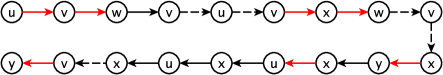
Figure 1: Illustrating marked edges (red), backtracks (black), and unmarked edges (dotted). The segments in this path are given by $S_{1}=(u,v,w,v)$, $S_{2}=(v,x,w)$, $S_{3}=(x,y,x,u,x,u,x)$, $S_{4}=(v,y)$. Here $S_{3}$ is a Type II segment with $k_{2}-k_{2}=2$ and $k_{3}-k_{2}=4$. The rest are Type I segments.

Definition 4.6 (Type I/II Segments and Paths).

Let $(i_{l},i_{l^{\prime}})$ be a segment with $r$ marked edges. Suppose $l=k_{1}<k_{2}<\cdots k_{r+1}=l^{\prime}$ be integers such that $(i_{k_{r^{\prime}}},i_{k_{r^{\prime}}+1})$ for $1\leq{r^{\prime}}\leq r$ constitute the set of all marked edge. Then $(i_{l},i_{l^{\prime}})$ is said to be a Type II segment if $k_{r^{\prime}+1}-k_{r^{\prime}}$ is an even number for $1\leq r^{\prime}\leq r$. In all other cases, $(i_{l},i_{l^{\prime}})$ is said to be a Type I segment. Intuitively, a Type II segment just represents going back and forth on the same vertex. In Figure 1, the third segment is Type II and the rest of the segments are Type I. We say that a path $p$ is a Type I path if there is at least one Type I segment in it. Otherwise, we call it a Type II path. Notice that Type II path may not have any segment.

Definition 4.7.

We call a path $p$ saturated if all the edges in $p$ are part of some segment, i.e., there are no unmarked edges in a saturated path.

We now state the following elementary lemma which will be used throughout:

Lemma 4.8.

There are at most $n^{r-1}$ ways to choose marked vertices for a Type I path with $r$ marked edges, and there are at most $n^{r}$ ways to do the same for a Type II path with $r$ marked edges.

Proof.

Let us focus only on a path $p$ that is saturated, since we want to maximize the choice of marked vertices and they can only be found by walking through a marked edge. Consider the path $p$, and note that the endpoints of $p$ are fixed at $i,j$, and all the edges are either marked or is a backtrack. Let $(i_{k_{\alpha}},i_{k_{\alpha}+1})$ with $1\leq\alpha\leq r$ be the marked edges. We construct a graph $H_{p}$ using only the marked edges (ignoring their orientation). Since $p$ is saturated, we have $H_{p}$ is connected, and also the vertices of $H_{p}$ (except possibly $i,j$) are marked vertices. If $p$ is Type II, then $H_{p}$ is a star centered at $i$ having $r$ edges, and $j$ can either be $i$ or be one of the leaves. Thus the vertices except $i,j$ can be chosen in at most $n^{r}$ ways. If $p$ is Type I, in order to get the maximum number of vertices in $H_{p}$, one can have $H_{p}$ to be a tree if $i\neq j$ or a unicyclic graph if $i=j$. In both cases, there are at most $r-1$ vertices (other than $i,j$) to choose, and these can be chosen in $n^{r-1}$ ways. ∎

To complete the proof of Proposition 4.2, let $E_{m,r}$ denote the summands in (4.7) restricted to the case that there are $r$ Type I segments, so that

$$E_{m}=\sum_{r=r_{*}(m)}^{r^{*}(m)}E_{m,r},$$

where, given $m$, $[r_{*}(m),r^{*}(m)]$ denotes the possible range of $r$. The analysis will consist of two steps. In the first step, we analyze $E_{m,r_{*}(m)}$. Subsequently, we will show that $E_{m,r}$ is much smaller than $E_{m,r_{*}(m)}$ for $r>r_{*}(m)$.

Intuitively, $E_{m,r_{*}(m)}$ is the largest term as minimizing the number of Type I segments leads to maximizing the number of choices for marked vertices. This can be seen from Lemma 4.8 which says that there are at most $r-1$ marked vertices to choose for a Type I segment with $r$ marked edges. In contrast, for a Type II segment we have an upper bound of $r$ choices for $r$ marked edges.

4.1.1 Computing $E_{m,r_{*}(m)}$.

We first find an expression of $r_{*}(m)$. Note the following:

Observation 4.9.

A Type I path has maximum number of marked edges if there is only one Type I segment having $t$ marked edges. We refer to these paths maximal Type I paths. (Thus, maximal paths are saturated).

Observation 4.10.

For a Type II path, let $h=h(t,i,j)$ be the maximum number of marked edges. Note that each marked edge in a Type II segment has at least one backtrack. We refer to such paths as maximal Type II paths. Note that $h=t/2$ if $t$ is even and $i=j$ as each marked edge in a Type II segment has at least one backtracking edge. If $t$ is even and $i\neq j$ then $h=(t-2)/2$ as Type II segments must start and end at the same vertex and Type II segments are of an even length. If $t$ is odd and $i\neq j$, then $h=(t-1)/2$ marked edges. If $t$ is odd and $i=j$ then it may have a maximum of $(t-3)/2$ marked edges. In particular for the last case, we cannot have $(t-1)/2$ marked edges as if that were the case then the first or the last edge in the path would be a self-loop at node $i$ which has probability $0$ in our model. We can also note that as a result, we cannot have a Type II path when $t=3$ and $i=j$ and we take $h=0$ in the case. Note that $h\leq\phi(t)=\lfloor t/2\rfloor$ for $t\geq 3$, where $\phi(t)$ is defined in Theorem 3.1.

We have that for the case of $r$ Type I segments, the number of marked edges satisfy $m\leq rt+(k-r)h$. Let

$$f(r):=rt+(k-r)h,\quad 0\leq r\leq k.$$

Then $r_{*}(m)$ is obtained by inverting $f$ as described below:

Lemma 4.11.

$r_{*}(m)=\max\{0,\lfloor\frac{m-kh}{t-h}\rfloor\}$.

Proof.

Let $f(r_{0}-1)<m\leq f(r_{0})$ for some $r_{0}\geq 1$. We would like to put as many edges in Type I segments as possible to minimize the number of Type I segments. However, since each path has length $t$ and $m>(r_{0}-1)t$, we need $r_{0}$ Type I segments, so that $r_{*}(m)\geq r_{0}$. Also, this lower bound is attained by taking $r_{0}-1$ many maximal Type I paths and another Type I path that is not maximal. If $m\leq f(0)$, then we can get away with having no Type I segments. This completes the proof. ∎

Next we count the possible ways of rearranging the Type I segments in $k$ paths.

Lemma 4.12.

Given $m$ marked edges and $r_{*}(m)$ Type I segments, the number of configurations of Type I, II segments and unmarked edges $N_{m,r_{*}(m)}$ satisfies

$$N_{m,r_{*}(m)}\leq\binom{k}{r_{*}(m)}k^{f(r_{*}(m))-m}3^{k-r_{*}(m)}C^{f(r_{*}(m))-m}.$$

Proof.

We treat four cases separately:

Case I: $m=f(r_{0})$ for some $1\leq r_{0}\leq k$. $r_{*}(m)=r_{0}$. If $m=f(r_{0})$, then we must take $r_{0}$ paths to place the $r_{0}=r_{*}(m)$ Type I segments which can be chosen in $\binom{k}{r_{0}}$ ways. The rest of the Type II segments are placed in the remaining $k-r_{0}$ paths. The Type I, II paths have to be maximal in order to place these $m$ marked edges. We note that there are at most $t-2h$ unmarked edges in each of these Type II paths, which are not part of the segments, and these can be chosen in at most $m$ ways each. This is because each unmarked edge is chosen to be one of the $m$ marked edges. We also note that for each Type II path, there are $t-2h\leq 3$ ways of placing the Type II segment in the path. So the overall bound for Case I is

$$\binom{k}{r_{*}(m)}3^{(k-r_{*}(m))}.$$

Case II: $f(r_{0}-1)<m<f(r_{0})$ for some $1\leq r_{0}\leq k$. Again, we have $r_{*}(m)=r_{0}$. Let $l=f(r_{0})-m$. Then we need $r_{0}$ distinct paths to place the $r_{0}=r_{*}(m)$ Type I segments, which again can be chosen in $\binom{k}{r_{0}}$. However, in this case, these paths might not be maximal. Take $l_{1}$ and $l_{2}$ such that $l_{1}+l_{2}\leq l$, all except $l_{1}$ of the $r_{0}$ Type I paths are maximal and and all except $l_{2}$ of the $k-r_{0}$ Type II paths are maximal. We can choose these $l_{1}+l_{2}$ many non-maximal paths in at most $O(k^{l})$ ways. Also, note that we can have at most $2l$ more unmarked edges compared to the case of $m=f(r_{0})$. The total number of ways of arranging the segments and unmarked edges for the non-maximal paths is $O(C^{l})$, where $C$ is a constant that might depend on $t$. Thus the bound for this case is

$$\binom{k}{r_{*}(m)}k^{l}3^{(k-r_{*}(m))}C^{l}.$$

Case III: $m=f(0)$. The same argument and the bound as Case I holds here. We note that this case does not occur if $h=0$.

Case IV: $m<f(0)$. Thus $m=f(0)-l$ for $l>0$. Note that this case also does not occur if $h=0$. Recall that for $m=f(0)$ case, all the paths have Type II segments containing $h$ marked edges. We would like to count the configurations for $m=f(0)-l$ marked edges with no Type I segments. We note that then there exist $1\leq u\leq l$ paths such that they have less than $h$ marked edges and the rest of the paths have $h$ marked edges. We can choose the $u$ paths in at most $O(k^{l})$ ways. We can then arrange segments in these $l$ paths in $C^{l}$ ways. Note that we can have at most $2l$ more unmarked edges for this case compared to the $m=f(0)$ case. The overall bound for this case is $(Ck)^{l}3^{k}$. ∎

We are now ready to prove asymptotics of $E_{m,r_{*}(m)}$.

Lemma 4.13.

$\sum_{m<kt}E_{m,r_{*}(m)}=o(U_{b}^{k})$.

Proof.

Let us start by noting that $U_{b}=\Theta(n^{t-1}\rho_{n}^{t})$. The number of choices of segments is given by Lemma 4.12. Since we have $r_{*}(m)$ Type I segments, we must have at least $s(m)=\max\left\{r_{*}(m)-(f(r_{*}(m))-m),0\right\}$ maximal Type I segments, with each of them having probability at most $U_{b}$. In the rest, we have one Type I segment. Thus by Lemma 4.8, the vertices in the rest of the paths can be chosen in at most $n^{m-ts(m)-(r_{*}(m)-s(m))}$ ways. Also the $m-ts(m)$ many remaining marked edges give us a contribution of at most $(C\rho_{n})^{m-ts(m)}$. The number of unmarked edges is specified in each of the cases in the proof of Lemma 4.12 above. Combining all these, we get

$$E_{m,r_{*}(m)} \leq\binom{k}{r_{*}(m)}k^{f(r_{*}(m))-m}3^{k-r_{*}(m)}C^{f(r_{*}(m))-m}$$

$$\quad\times U_{b}^{s(m)}n^{m-ts(m)-(r_{*}(m)-s(m))}\rho_{n}^{m-ts(m)}$$

$$\quad\times m^{(k-r_{*}(m))\cdot(t-2h)+2(f(r_{*}(m))-m)}.$$

Using these bounds we see that with the choice of $k=\lceil\log n\rceil$

$$\sum_{l=0}^{t-h-1}E_{f(r_{0})-l,r_{\star}(f(r_{0})-l)} =E_{f(r_{0})-l,r_{\star}(f(r_{0})-l)}\left(1+O\left(\frac{k^{3}}{n\rho_{n}}\right)\right),\quad r_{0}\geq 1,$$

$$\sum_{l=0}^{f(0)-1}E_{f(0)-l,r_{\star}(f(0)-l)} =E_{f(0)-l,r_{\star}(f(0)-l)}\left(1+O\left(\frac{k^{3}}{n\rho_{n}}\right)\right),$$

$$\sum_{r_{0}=0}^{k}E_{f(r_{0}),r_{\star}(f(r_{0}))} =E_{f(k),r_{\star}(f(k))}\left(1+O\left(\frac{k^{1+t-2h}(n\rho_{n})^{h}}{n^{t-1}\rho_{n}^{t}}\right)\right).$$

These bounds in turn imply that

$$\sum_{m=1}^{kt-1}E_{m,r_{*}(m)}=o\left(U_{b}^{k}\right).$$

∎

4.1.2 Computing $E_{m,r}$ for $r>r_{*}(m)$.

We start by noting the additional number of configurations with $r$ Type I segments as compared to Lemma 4.8.

Lemma 4.14.

Given $m$ marked edges and $r$ Type I segments, let $N_{m,r}$ be the number of configurations of Type I, II segments and unmarked edges. Then, for any $r>r_{*}(m)$,

$$N_{m,r}\leq N_{m,r_{*}(m)}\times(Ck)^{(r-r_{*}(m))(t+1)}.$$

Proof.

Figure 2: Example of a splitting a segment. $(a)$ The original configuration of the segments in the chosen path. The edges in the two segments are colored red and blue respectively. The edges are also labeled by M, B and U if the edge is a marked edge, a backtrack of a marked edge and an unmarked edge respectively. The dotted line indicates the location of the split. $(b),(c)$ Two examples of configurations after the splitting the segment. The two new segments are colored by green and violet.

Let $T_{r}$ be the set of all configurations of $m$ marked edges and $r$ Type I segments. Note that a “configuration” here only specifies location of marked edges, segments, and the unmarked edges. The backtracks of the marked edges are already specified. We will inductively bound $T_{r+1}$ in terms $T_{r}$. For that, we consider two cases depending on whether the elements of $T_{r+1}$ has a Type I path with two Type I segments or not. In both cases, we will find a relation between $T_{r}$ to $T_{r+1}$.

Case I.

Consider elements of $T_{r+1}$ that has a Type I path with two Type I segments. Let us call this subset $T_{r+1}^{\scriptscriptstyle I}$. We consider the elements in $T_{r}$ which will be related to these elements in $T_{r+1}^{\scriptscriptstyle I}$. Let $T_{r}^{\scriptscriptstyle I}\subset T_{r}$ consisting of configuration such that there is at least one path $p$ so that the following hold:

1. Extra unmarked edges. $p$ has $l$ segments and $l^{\prime}\geq l$ unmarked edges for some $l,l^{\prime}\geq 1$.

2. Well-splittable. Suppose $p$ has a Type I segment $(i_{l},i_{l+1},\ldots,i_{l^{\prime}})$ with marked edges given by $(i_{k_{s}},i_{k_{s}+1})$ for $l\leq k_{s}<l^{\prime}$, $1\leq s\leq m^{\prime}$, $m^{\prime}\geq 1$, and the number of $s$ with $k_{s+1}-k_{s}$ being odd is at least $2$.

Note that a path with $l$ segments can be formed by just putting $l-1$ unmarked edges between segments. The first condition ensures that we have extra $l^{\prime}-l+1$ of them. We will put these extra unmarked edges inside segments to split them. Regarding condition 2, notice that a Type I segment always has one of the $k_{s+1}-k_{s}$ being odd (by definition), but the well-splittable condition requires $k_{s+1}-k_{s}$ to be odd additionally in a second place. This allows us to split a well-splittable Type I segment into two Type I segments. For example, the blue segment in Figure 3 (a) is well-splittable and it can be split into two parts with $k_{s+1}-k_{s}$ being odd. We will split the segment by moving an unmarked edge in between as illustrated in Figure 3.

The general description for splitting is that given a path with extra marked edges and well-splittable property, we can think of unmarked edges as “bars”, and segments as “labelled balls”. The well-splittable segment is viewed as two Type I sub-segments and corresponds to two “labelled balls”. Permute these bars and balls such that there is at least one bar between any two labelled balls (bars can be adjacent). Also, there may be multiple ways to split well-splittable segment and we consider all possible such splits. This creates multiple elements in $T_{r+1}^{\scriptscriptstyle I}$ from an element in $T_{r}^{\scriptscriptstyle I}$. See Figure 2 (b), (c) for two possible elements. Moreover, we can get preimages of all the elements in $T_{r+1}^{\scriptscriptstyle I}$,. To do this, we can first take a path with two Type I segments, rearranging the segments so that two Type I segments appear one after another. Then we can remove the unmarked edges between them, which joins the two Type I segments. The removed unmarked edges can be placed in other places adjacent to an unmarked edge. This is basically the inverse operation of the above splitting constructions.

We can note there are $O(k)$ preimages in total of an element in $T_{r+1}^{\scriptscriptstyle I}$, where the factor $k$ comes from choice of the path $p$ and the rest of the choices for permuting unmarked edges and segments are $O(1)$ as they are functions of only $t$ which is bounded. Thus,

$$|T_{r+1}^{\scriptscriptstyle I}|\leq O(k)\times|T_{r}^{\scriptscriptstyle I}|\leq O(k)\times|T_{r}|.$$

Case II.

Figure 3: Example of the second construction for the case of $t=4$, $m=4$ and $s=1$. The marked edges are colored red. The letters M, B and U denote a marked edge, a backtrack of a marked edge and an unmarked edge respectively. $(a)$ The top path is the chosen path where we would place a Type I segment. The second path contains one Type I segment and the bottom path is a Type II path. $(b),(c)$ Two examples of new configurations from the construction. In both the cases the top path now has a Type I segment and the middle path continues to have a Type I segment.

We next relate arrangements of marked edges where there is at most one Type I segment per path. We denote such arrangements as $T_{r+1}^{\scriptscriptstyle II}\subset T_{r+1}$. Let $T_{r}^{\scriptscriptstyle II}$ be the set of all ways of specifying locations of segments such that there are a total of $r$ Type I segments and each of the Type I segments is placed on distinct paths. Suppose that $r+1\leq\min(k,m)$ and $r\geq r_{\star}(m)$. Then we give a multi-map from $T_{r}^{\scriptscriptstyle II}$ onto $T_{r+1}^{\scriptscriptstyle II}$ using a construction. The condition $r+1\leq m$ is necessary so that $T_{r+1}^{\scriptscriptstyle II}$ is non-empty as we must have at least $r+1$ marked edges in order to have $r+1$ paths each having a Type I segment. The condition $r+1\leq k$ is also necessary for $T_{r+1}^{\scriptscriptstyle II}$ to be non-empty as we must have at least $r+1$ distinct paths to place the $r+1$ Type I segments. The last condition $r\geq r_{\star}(m)$ is to ensure that $T_{r}^{\scriptscriptstyle II}$ is non-empty. To fix notation, let $S_{1}(l)$ be the set of all ways of arranging $l$ marked edges in one path such that there is at least one Type I segment in the path. Similarly, let $S_{2}(l)$ be the set of all ways of arranging $l$ marked edges in one path such that there are no Type I segments in the path. We now describe the construction. Let $A\in T_{r}^{\scriptscriptstyle II}$ and choose a path $p$ not containing a Type I segment. We can do so as $r+1\leq k$. Suppose $p$ has $l\geq 0$ marked edges. Choose $0\leq u_{1}+u_{2}\leq t-l$ paths where $u_{1}$ of the paths are paths containing Type I segments with at least two marked edges and the rest $u_{2}$ paths are paths which are distinct from $p$, do not contain Type I segments, and contain at least one marked edge. If $l=0$ we require $u_{1}+u_{2}>0$. It is feasible to choose such path(s) as $r+1\leq m$. Suppose the $u_{1}$ paths are labeled as $q_{1},q_{2},\ldots,q_{u_{1}}$ and the $u_{2}$ paths indices $q^{\prime}_{1},q^{\prime}_{2},\ldots,q^{\prime}_{u_{2}}$. Suppose these paths have $l_{q_{1}},l_{q_{2}},\cdots,l_{q_{u_{1}}}$ and $l_{q^{\prime}_{1}},l_{q^{\prime}_{2}},\cdots,l_{q^{\prime}_{u_{2}}}$ marked edges respectively. Let $v_{q_{1}},v_{q_{2}},\cdots,v_{q_{u_{1}}}$ be such that $0<v_{q_{i}}<l_{q_{i}}$. Similarly let $v_{q^{\prime}_{1}},v_{q^{\prime}_{2}},\cdots,v_{q^{\prime}_{u_{2}}}$ be such that $0<v_{q^{\prime}_{i}}\leq l_{q^{\prime}_{i}}$. We require $\sum_{i}v_{q_{i}}+\sum_{i}v_{q^{\prime}_{i}}\leq t-l$. Then we modify the arrangements of marked edges in the paths so that the new arrangements for the sequence of paths $(p,q_{1},q_{2},\ldots,q_{u_{1}},q^{\prime}_{1},q^{\prime}_{2},\ldots,q^{\prime}_{u_{2}})$ is any element of

$$S_{1}\left(l+\sum_{i}v_{q_{i}}+\sum_{i}v_{q^{\prime}_{i}}\right)\times\left(\prod_{i=1}^{u_{1}}S_{1}(l_{q_{i}}-v_{q_{i}})\right)\times\left(\prod_{i=1}^{u_{2}}S_{2}(l_{q^{\prime}_{i}}-v_{q^{\prime}_{i}})\right).$$

We keep the arrangements of marked edges in the rest $k-(1+u_{1}+u_{2})$ paths unchanged. This leads to multiple images of $A$ in $T_{r+1}^{\scriptscriptstyle II}$. We note that there are $O(k^{t+1})$ images of $A$ due to the choice of the paths and since the number of ways of choosing the new arrangements for the $1+u_{1}+u_{2}$ paths is $O(1)$ as $t$ is fixed. We also note that since we modify at most $t+1$ paths in this construction, the number of unmarked edges increases by at most $t(t+1)$.

Now we show that the multi-map given by the construction above is surjective onto $T_{r+1}^{\scriptscriptstyle II}$. For this, let $A^{\prime}\in T_{r+1}^{\scriptscriptstyle II}$. Let $p$ be a path containing a Type I segment. If $p$ has $l\leq h$ edges we choose an element in $x\in S_{2}(l)$. We can then see that $A^{\prime}$ is in the image of the element $A\in T_{r}^{\scriptscriptstyle II}$ where the path $p$ has the arrangement of marked edges given by $x$ and the rest of the paths have the same arrangement of marked edges as $A^{\prime}$. We note that since we have replaced the Type I segment in the path $p$ with a Type II segment, the element $A$ has one less Type I segment. Now suppose that $p$ has $l>h$ edges. Choose $u_{1}+u_{2}\leq l-h$ paths so that $u_{1}$ paths contain Type I segments and these paths are not equal to $p$ and, $u_{2}$ paths do not contain Type I segments segments. Suppose the $u_{1}$ paths are labeled as $q_{1},q_{2},\ldots,q_{u_{1}}$ and the $u_{2}$ paths are labeled as $q^{\prime}_{1},q^{\prime}_{2},\ldots,q^{\prime}_{u_{2}}$. Suppose that these paths have $l_{q_{1}},l_{q_{2}},\cdots,l_{q_{u_{1}}}$ and $l_{q^{\prime}_{1}},l_{q^{\prime}_{2}},\cdots,l_{q^{\prime}_{u_{2}}}$ marked edges respectively. We require that $l_{q_{i}}<t$ and $l_{q^{\prime}_{i}}<h$ i.e. that these chosen paths are not saturated. Let $v_{q_{1}},v_{q_{2}},\cdots,v_{q_{u_{1}}}$ be such that $0<v_{q_{i}}\leq t-l_{q_{i}}$. Similarly let $v_{q^{\prime}_{1}},v_{q^{\prime}_{2}},\cdots,v_{q^{\prime}_{u_{2}}}$ be such that $0<v_{q^{\prime}_{i}}\leq h-l_{q^{\prime}_{i}}$. We require that

$$\sum_{i=1}^{u_{1}}v_{q_{i}}+\sum_{i=1}^{u_{2}}v_{q^{\prime}_{i}}=l-h.$$

This is feasible as long as $r\geq r_{\star}(m)$. The above condition says that the chosen paths have enough spaces to move $l-h$ edges from path $p$ to the chosen paths. Choose a new arrangement $x$ of the marked edges for the sequence of paths $(p,q_{1},q_{2},\ldots,q_{u_{1}},q^{\prime}_{1},q^{\prime}_{2},\ldots,q^{\prime}_{u_{2}})$ from the set

$$S_{2}\left(h\right)\times\left(\prod_{i=1}^{u_{1}}S_{1}(l_{q_{i}}+v_{q_{i}})\right)\times\left(\prod_{i=1}^{u_{2}}S_{2}(l_{q^{\prime}_{i}}+v_{q^{\prime}_{i}})\right).$$

Then keeping the arrangements of marked edges of the rest of the paths the same as in $A^{\prime}$ and choosing the arrangements for the chosen paths as $x$, we have a preimage $A\in T_{r}^{\scriptscriptstyle II}$ under the construction described above.

From the two constructions above we have

$$|T_{r+1}|\leq O(k)|T_{r}|+O(k^{t+1})|T_{r}|.$$ (4.9)

∎

We can now compute asymptotics for $E_{m,r}$.

Lemma 4.15.

$\sum_{r=r_{*}(m)}^{r^{*}(m)}E_{m,r}=E_{m,r_{*}(m)}(1+o(1))$.

Proof.

We start by giving a bound for $E_{m,r}$. The probability of the $m$ marked edges is bounded by $\rho_{n}^{m}$. By Lemma 4.8, the upper bound for the number of marked edges is $m-r$ as there are $r$ Type I segments. Let

$$u(m)=(k-r_{*}(m))\cdot(t-2h)+2(f(r_{*}(m))-m),$$

be the upper bound for the number of unmarked edges for the case of $r_{*}(m)$ segments obtained from the proof of Lemma 4.13. Then by the two constructions in Lemma 4.14, the number of unmarked edges for the case of $r$ Type I segments is at most $u(m)+(r-r_{*}(m))\cdot(t(t+1))$. Combining these we have

$$E_{m,r}\leq N_{m,r}n^{m-r}\rho_{n}^{m}m^{u(m)+(r-r_{*}(m))\cdot t(t+1)}.$$

Then by using Lemma 4.14 we have

$$\sum_{r=r_{*}(m)}^{r^{*}(m)}E_{m,r}=E_{m,r_{*}(m)}\sum_{r=r_{*}(m)}^{r^{*}(m)}\left(\frac{O(k^{t+1})\cdot m^{t(t+1)}}{n}\right)^{r-r_{*}(m)}=E_{m,r_{*}(m)}(1+o(1)).$$

∎

By Lemmas 4.13 and 4.15 we then have

$$\sum_{m<kt}E_{m}\leq C\sum_{m<kt}E_{m,r_{*}(m)}=o(U_{b}^{k}).$$

This completes the proof of Proposition 4.2.

4.2 Concentration of path counts

In this section, we prove concentration of $Y_{b}$ defined in (4.4). Let us start with a general result which we will apply for indicator random variables appearing in paths:

Lemma 4.16.

Let $\mathcal{E}$ be a finite set and let $\xi_{e}$ be indicator random variables for $e\in\mathcal{E}$ with $\pi_{e}=\mathbb{P}(\xi_{e}=1)>0$. For a subset $S\subset\mathcal{E}$, we define $\xi_{S}:=\prod_{e\in S}\xi_{e}$. Suppose $S_{1},S_{2},\ldots S_{k}$ be non-empty subsets of $\mathcal{E}$ and let $n_{e}:=|\{j\in[k]:e\in S_{j}\}|$. Let $\mathcal{E}_{1}:=\{e\in\cup_{j=1}^{k}S_{j}:n_{e}=1\}$ and $\mathcal{E}_{2}=\left(\cup_{j=1}^{k}S_{j}\right)\backslash\mathcal{E}_{1}$. Then we have

$$\bigg{|}\mathbb{E}\prod_{j=1}^{k}(\xi_{S_{j}}-\mathbb{E}\xi_{S_{j}})\bigg{|}\leq\bigg{(}\prod_{e\in\mathcal{E}_{1}}\pi_{e}\bigg{)}\times\bigg{(}\prod_{e\in\mathcal{E}_{2}}\pi_{e}(1+\pi_{e})\bigg{)}.$$ (4.10)

Proof.

Let $S_{j}^{\scriptscriptstyle(1)}\subseteq S_{j}^{\scriptscriptstyle(2)}\subseteq S_{j}$ and $m=|\cup_{j=1}^{k}S_{j}^{\scriptscriptstyle(1)}|$. We define $n_{e}^{\scriptscriptstyle(1)}$ and $\mathcal{E}_{1}^{\scriptscriptstyle(1)}$ similarly as $n_{e}$, $\mathcal{E}_{1}$ but now with sets $S_{j}^{\scriptscriptstyle(1)}$. We prove by induction on $m$ that, for all possible choices of $S_{j}^{\scriptscriptstyle(1)},S_{j}^{\scriptscriptstyle(2)}$, — E∏_j=1^k (ξ_S_j^(1) - Eξ_S_j^(2) ) — ≤(∏_e ∈E_1^(1) π_e) ×(∏_e ∈E_2^(1) π_e (1 + π_e)). Throughout, we use the convention that a product over an empty index set is $1$. For the induction base case, suppose $m=1$. Let $e$ be the only element in $\cup_{i=1}^{k}S_{j}^{\scriptscriptstyle(1)}$ and without loss of generality let $e\in S_{j}^{\scriptscriptstyle(1)}$ for $1\leq j\leq n_{e}^{\scriptscriptstyle(1)}$. If $n_{e}^{\scriptscriptstyle(1)}=1$, then

$$\mathbb{E}\big{(}\xi_{S_{1}^{\scriptscriptstyle(1)}}-\mathbb{E}\xi_{S_{1}^{\scriptscriptstyle(2)}}\big{)}=\pi_{e}\big{(}1-\mathbb{E}\xi_{S_{1}^{\scriptscriptstyle(2)}}^{\prime}\big{)}\leq\pi_{e},$$

where $\xi_{S_{1}^{\scriptscriptstyle(2)}}^{\prime}:=\xi_{S_{1}^{\scriptscriptstyle(2)}\setminus\{e\}}$. The terms with $S_{j}^{\scriptscriptstyle(1)}=\varnothing$ can be bounded by 1. This shows the base case for $m=1$ and $n_{e}^{\scriptscriptstyle(1)}=1$. If $n_{e}^{\scriptscriptstyle(1)}>1$, then

$$\mathbb{E}\bigg{[}\prod_{j=1}^{n_{e}^{\scriptscriptstyle(1)}}\big{(}\xi_{S_{j}^{\scriptscriptstyle(1)}}-\mathbb{E}\xi_{S_{j}^{\scriptscriptstyle(2)}}\big{)}\bigg{]}=\mathbb{E}\bigg{[}\prod_{j=1}^{n_{e}^{\scriptscriptstyle(1)}}\big{(}\xi_{e}-\mathbb{E}\xi_{S_{j}^{\scriptscriptstyle(2)}}\big{)}\bigg{]}$$

$$=\pi_{e}\cdot\prod_{j=1}^{n_{e}^{\scriptscriptstyle(1)}}\big{(}1-\mathbb{E}\xi_{S_{j}^{\scriptscriptstyle(2)}}\big{)}+(1-\pi_{e})\cdot\prod_{j=1}^{n_{e}^{\scriptscriptstyle(1)}}\big{(}-\mathbb{E}\xi_{S_{j}^{\scriptscriptstyle(2)}}\big{)}\leq\pi_{e}+(\pi_{e})^{n_{e}^{\scriptscriptstyle(1)}}\leq\pi_{e}(1+\pi_{e}).$$

This completes the proof of the base case $m=1$.

Next let $m>1$. We will split in two cases depending on whether $\mathcal{E}_{1}^{\scriptscriptstyle(1)}\neq\varnothing$ and $\mathcal{E}_{1}^{\scriptscriptstyle(1)}=\varnothing$. First, if $\mathcal{E}_{1}^{\scriptscriptstyle(1)}\neq\varnothing$, then pick an element $e\in\mathcal{E}_{1}^{\scriptscriptstyle(1)}$. Note that $e$ can only be in one of $S_{j}^{\scriptscriptstyle(1)}$’s, and without loss of generality let $e\in S_{1}^{\scriptscriptstyle(1)}$. Let $\mathcal{F}_{e}$ is the minimum sigma-algebra with respect to which $(\xi_{f})_{f\neq e}$ are measurable, and analogously to before, define $\xi_{S_{1}^{\scriptscriptstyle(1)}}^{\prime}:=\xi_{S_{1}^{\scriptscriptstyle(1)}\setminus\{e\}}$ and $\xi_{S_{1}^{\scriptscriptstyle(2)}}^{\prime}:=\xi_{S_{1}^{\scriptscriptstyle(2)}\setminus\{e\}}$. Taking iterated conditional expectation with respect to $\mathcal{F}_{e}$, we get

$$\mathbb{E}\bigg{[}\prod_{j\in[k]:S_{j}^{\scriptscriptstyle(2)}\neq\varnothing}\big{(}\xi_{S_{j}^{\scriptscriptstyle(1)}}-\mathbb{E}\xi_{S_{j}^{\scriptscriptstyle(2)}}\big{)}\bigg{]}=\pi_{e}\cdot\mathbb{E}\bigg{[}\big{(}\xi_{S_{1}^{\scriptscriptstyle(1)}}^{\prime}-\mathbb{E}\xi_{S_{1}^{\scriptscriptstyle(2)}}^{\prime}\big{)}\prod_{j\in\{2,3,\ldots k\}:S_{j}^{\scriptscriptstyle(2)}\neq\varnothing}\big{(}\xi_{S_{j}^{\scriptscriptstyle(1)}}-\mathbb{E}\xi_{S_{j}^{\scriptscriptstyle(2)}}\big{)}\bigg{]}.$$

Now we can conclude (4.2) by induction step using $S_{1}^{\scriptscriptstyle(1)}\setminus\{e\}$, $S_{1}^{\scriptscriptstyle(2)}\setminus\{e\}$ and $S_{j}^{\scriptscriptstyle(1)}$, $S_{j}^{\scriptscriptstyle(2)}$ for $j\geq 2$, and noting that $\mathcal{E}_{1}^{\scriptscriptstyle(2)}$ is unchanged in this new set up.

Next suppose that $\mathcal{E}_{1}^{\scriptscriptstyle(1)}=\varnothing$. Pick any $e\in\mathcal{E}_{2}^{\scriptscriptstyle(1)}$. Then $n_{e}^{\scriptscriptstyle(1)}>1$ and without loss of generality let $e\in S^{\scriptscriptstyle(1)}_{j}$ for $1\leq j\leq n_{e}^{\scriptscriptstyle(1)}$. We again take iterated conditional expectation with respect to $\mathcal{F}_{e}$ to get &E[∏_j∈[k]: S_j^(2) ≠∅ (ξ_S_j^(1) - Eξ_S_j^(2) ) ]
=E[∏_j ∈{ n_e^(1) + 1,…,k} : S_j^(2) ≠∅ (ξ_S_j^(1) - Eξ_S_j^(2) ) E[ ∏_j=1 ^n_e^(1) (ξ_S_j^(1) - Eξ_S_j^(2) )  — F_e ] ]. We simplify

$$\mathbb{E}\bigg{[}\prod_{j=1}^{n_{e}^{\scriptscriptstyle(1)}}\big{(}\xi_{S_{j}^{\scriptscriptstyle(1)}}-\mathbb{E}\xi_{S_{j}^{\scriptscriptstyle(2)}}\big{)}\ \Big{|}\mathcal{F}_{e}\bigg{]}=\pi_{e}\cdot\prod_{j=1}^{n_{e}^{\scriptscriptstyle(1)}}\big{(}\xi_{S_{j}^{\scriptscriptstyle(1)}}^{\prime}-\mathbb{E}\xi_{S_{j}^{\scriptscriptstyle(2)}}\big{)}+(1-\pi_{e})\prod_{j=1}^{n_{e}^{\scriptscriptstyle(1)}}\big{(}-\mathbb{E}\xi_{S_{j}^{\scriptscriptstyle(2)}}\big{)}.$$ (4.11)

Suppose that $m-l=\lvert\cup_{j=n_{e}^{\scriptscriptstyle(1)}+1}^{k}S^{\scriptscriptstyle(2)}_{j}\rvert$ for some $l\geq 1$ (we have $l\geq 1$ since $e$ is not in the union). For the second term in (4.11), we have

$$\bigg{|}(1-\pi_{e})\prod_{j=1}^{n_{e}^{\scriptscriptstyle(1)}}(-\mathbb{E}\xi_{S_{j}^{\scriptscriptstyle(2)}})\bigg{|}\leq\pi_{e}^{n_{e}^{\scriptscriptstyle(1)}-1}\prod_{f\in\cup_{j=1}^{n_{e}^{\scriptscriptstyle(1)}}S^{\scriptscriptstyle(2)}_{j}}\pi_{f}=:Z_{1},$$

as the term $\xi_{e}$ is repeated $r$ times. We bound the term in (4.2) outside conditional expectation by induction. If we consider the sets $S_{j}^{\scriptscriptstyle(1)}$, $S_{j}^{\scriptscriptstyle(2)}$ for $j>n_{e}^{\scriptscriptstyle(1)}$ with $S_{j}^{\scriptscriptstyle(2)}\neq\varnothing$ and create the sets $\tilde{\mathcal{E}}_{1}$ and $\tilde{\mathcal{E}}_{2}^{\prime}$ analogously to $\mathcal{E}_{1}^{\scriptscriptstyle(1)}$, $\mathcal{E}_{1}^{\scriptscriptstyle(2)}$ when restricted to this smaller class of subsets. Then

$$\bigg{|}\mathbb{E}\bigg{[}\prod_{j\in\{n_{e}^{\scriptscriptstyle(1)}+1,\dots,k\}:S_{j}^{\scriptscriptstyle(2)}\neq\varnothing}\big{(}\xi_{S_{j}^{\scriptscriptstyle(1)}}-\mathbb{E}\xi_{S_{j}^{\scriptscriptstyle(2)}}\big{)}\bigg{]}\bigg{|}\leq\prod_{f\in\tilde{\mathcal{E}}_{1}}\pi_{f}\prod_{f\in\tilde{\mathcal{E}}_{2}}\pi_{f}(1+\pi_{f})=:Z_{2}.$$

Hence, the term in (4.2) is at most

$$\pi_{e}\bigg{|}\mathbb{E}\bigg{[}\prod_{j\in\{n_{e}^{\scriptscriptstyle(1)}+1,\dots,k\}:S_{j}^{\scriptscriptstyle(2)}\neq\varnothing}\big{(}\xi_{S_{j}^{\scriptscriptstyle(1)}}-\mathbb{E}\xi_{S_{j}^{\scriptscriptstyle(2)}}\big{)}\prod_{j=1}^{n_{e}^{\scriptscriptstyle(1)}}\big{(}\xi_{S_{j}^{\scriptscriptstyle(1)}}^{\prime}-\mathbb{E}\xi_{S_{j}^{\scriptscriptstyle(2)}}\bigg{]}\bigg{|}+Z_{1}Z_{2}$$

$$\leq\pi_{e}\cdot\left(\prod_{f\in\mathcal{E}_{1}^{\scriptscriptstyle(1)}}\pi_{f}\cdot\prod_{f\in\mathcal{E}_{2}^{\scriptscriptstyle(1)}\setminus\{e\}}\pi_{e}(1+\pi_{e})\right)+\pi_{e}^{n_{e}^{\scriptscriptstyle(1)}-1}\prod_{f\in\cup_{j=1}^{n_{e}^{\scriptscriptstyle(1)}}S^{\scriptscriptstyle(2)}_{j}}\pi_{f}\prod_{f\in\tilde{\mathcal{E}}_{1}}\pi_{f}\prod_{f\in\tilde{\mathcal{E}}_{2}^{\prime}}\pi_{f}(1+\pi_{f}).$$

The last term above is at most the bound in (4.2), which follows by noting that the second term has a factor of $(\pi_{e})^{n_{e}^{\scriptscriptstyle(1)}}$ with $n_{e}^{\scriptscriptstyle(1)}\geq 2$, and for each of the variables $f\in\mathcal{E}_{1}^{\scriptscriptstyle(1)},f\neq e$ the second term has a factor smaller or equal to $\pi_{f}$, and for each of the variables $f\in\mathcal{E}_{1}^{\scriptscriptstyle(1)}$ the second term has a factor smaller or equal to $\pi_{f}(1+\pi_{f})$. This completes the proof. ∎

We now prove the following concentration result for $Y_{b}$:

Proposition 4.17.

Let $t_{\scriptscriptstyle L}=t_{\scriptscriptstyle U}=t\geq 3$ be given and $k=\lceil\log n\rceil$. Suppose that (3.1) holds. Then we have

$$\mathbb{P}\left(|Y_{b}-\mathbb{E}Y_{b}|>\delta\mathbb{E}Y_{b}\right)=O(n^{-c}),$$

where $\delta=\Theta((\log n)^{-\eta})$ for some $\eta>0$, and $c>0$ is any real number.

Proof.

We will be using notation and terminology from proof of Proposition 4.2. By Markov’s inequality, and using Proposition 4.1,

$$\mathbb{P}\left(|Y_{b}-\mathbb{E}Y_{b}|>\delta\mathbb{E}Y_{b}\right) \leq\frac{\mathbb{E}(Y_{b}-\mathbb{E}Y_{b})^{2k}}{\delta^{2k}\left(\mathbb{E}Y_{b}\right)^{2k}}\leq\frac{\mathbb{E}(Y_{b}-\mathbb{E}Y_{b})^{2k}}{\delta^{2k}(L_{b})^{2k}},$$ (4.12)

and moreover,

$$\mathbb{E}(Y_{b}-\mathbb{E}Y_{b})^{2k} =\mathbb{E}\bigg{(}\sum_{p\in\mathcal{P}_{b}}(X_{p}-\mathbb{E}X_{p})\bigg{)}^{2k}=\sum_{(p_{1},p_{2},\ldots,p_{2k}):p_{l}\in\mathcal{P}_{b}}\mathbb{E}\prod_{l=1}^{2k}(X_{p_{l}}-\mathbb{E}X_{p_{l}}).$$ (4.13)

Fix an ordered sequence $(p_{1},p_{2},\ldots,p_{2k})$. We can first note that $\mathbb{E}\prod_{l=1}^{2k}(X_{p_{l}}-\mathbb{E}X_{p_{l}})$ is equal to $0$ if there is a path $p_{l}$ which does not have any edges in common with the other $2k-1$ paths. Suppose now that each of the paths share at least one edge with some other path. Then the minimum number of unmarked edges or repeats of edges is at least $k$. This minimum $k$ arises from the worst case where we have $k$ pairs of paths with each pair having one edge in common. Thus, the number of marked edges $m\leq 2kt-k$.

To bound $\mathbb{E}\prod_{l=1}^{2k}(X_{p_{l}}-\mathbb{E}X_{p_{l}})$, we use Lemma 4.16. For each marked edge $e$ with endpoints in block $b_{i}$ and $b_{i^{\prime}}$ between two nodes blocks $b_{i}$ and $b_{i^{\prime}}$, we assign a weight $w(e)=B_{b_{i},b_{i^{\prime}}}$. For each unmarked edge $e$, we assign a weight $w(e)=(1+B_{b_{i},b_{i^{\prime}}})$ instead. Then we can see by Lemma 4.16, $\mathbb{E}\prod_{l=1}^{2k}(X_{p_{l}}-\mathbb{E}X_{p_{l}})$ is bounded by the product of the weights on the edges in the $2k$ paths, i.e.,

$$\mathbb{E}\prod_{l=1}^{2k}(X_{p_{l}}-\mathbb{E}X_{p_{l}})\leq\prod_{e:e\text{ is marked}}w(e)\times\prod_{e:e\text{ is unmarked}}(1+w(e)).$$ (4.14)

We note that while bounding $E_{m}$ in the proof of Proposition 4.2, we bounded the probability of each of the marked edges by $w(e)$ as well. Let $E^{\prime}_{m}$ be the sum of summands in (4.13) corresponding to paths with $m$ marked edges. We use the bound $1+w(e)\leq 2$ for the weight on the unmarked edges and proceed as in the proof of Proposition 4.2 to have for $m\leq 2kt-k$:

$$E^{\prime}_{m} \leq C^{\prime}\binom{2k}{r_{*}(m)}(2k)^{f(r_{*}(m))-m}3^{2k-r_{*}(m)}C^{f(r_{*}(m))-m}$$

$$\quad\times U_{b}^{s(m)}n^{m-ts(m)-(r_{*}(m)-s(m))}\rho_{n}^{m-ts(m)}$$

$$\quad\times(2m)^{(2k-r_{*}(m))\cdot(t-2h)+2(f(r_{*}(m))-m)}.$$

Let $m_{0}$ be such that $m_{0}=f(r_{*}(m))$ and define $E^{\prime}_{m_{0}}$ with the same expression as above. Then bounding as in the proof of Proposition 4.2 we have from (4.13)

$$\mathbb{E}(Y_{b}-\mathbb{E}Y_{b})^{2k}\leq CE^{\prime}_{m_{0}}.$$

Thus, (4.12) together with the fact that $\frac{U_{b}}{L_{b}}=1+O(\frac{k}{n})$ yields

$$\mathbb{P}\left(|Y_{b}-\mathbb{E}Y_{b}|>\delta\mathbb{E}Y_{b}\right) \leq\frac{\binom{2k}{r_{*}(m)}3^{2k-r_{*}(m)}U_{b}^{r_{*}(m)}(n\rho_{n})^{m-tr_{*}(m)}(2m)^{(2k-r_{*}(m))\cdot(t-2h)}}{\delta^{2k}L_{b}^{2k}}$$

$$\leq\left(\frac{U_{b}}{L_{b}}\right)^{r_{*}(m)}\cdot\left(\frac{Ck^{1+t-2h}(n\rho_{n})^{h}\delta^{-\frac{2k}{2k-r_{*}(m)}}}{n^{t-1}\rho_{n}^{t}}\right)^{2k-r_{*}(m)},$$

$$\leq C\left(\frac{C(\log n)^{1+t-2h-2\eta(t-h)}(n\rho_{n})^{h}}{n^{t-1}\rho_{n}^{t}}\right)^{\lceil\log n\rceil(t-h)^{-1}}\leq n^{-c},$$

for any $c>0$ when (3.1) holds. This completes the proof of Proposition 4.17.

∎

5 Analysis of spectral clustering for DeepWalk

In this section, we first prove properties of the $M_{0}$ matrix in Section 5.1. In Section 5.2 we bound $\|M-M_{0}\|_{\scriptscriptstyle\mathrm{F}}$ and complete the proof of Theorem 3.1. Finally, we bound the number of misclassified nodes in Section 5.3 and complete the proof of Theorem 3.3.

5.1 Analysis of noiseless $M$-matrix

Recall the definition of the matrix $M_{0}$ from Section 2.3. Also recall that $\Theta_{0}$ is the matrix of true community assignments. Let $(\lambda_{i},v_{i})$, $1\leq i\leq K$ be the $K$ largest eigenvalue-eigenvector pairs of $M_{0}$, and let $V_{0}=(v_{1},\dots,v_{K})$. We will prove the following collection of claims for $M_{0}$ and its eigenspace:

Proposition 5.1.

1. There exists a full-rank matrix $Z_{0}\in\mathbb{R}^{K\times K}$ such that $M_{0}=\Theta_{0}Z_{0}\Theta_{0}^{T}$. Moreover, $(M_{0})_{ij}=\Theta(1)$ uniformly in $i,j\in[n]$.

2. We have $\lambda_{i}=\Theta(n)$ and there exists a full rank matrix $X_{0}\in\mathbb{R}^{K\times K}$ such that $V_{0}=\Theta_{0}X_{0}$.

3. If $i$ and $j$ are two nodes such that $g(i)\neq g(j)$, then we have

   $$\|(V_{0})_{i\star}-(V_{0})_{j\star}\|_{\scriptscriptstyle\mathrm{F}}=\sqrt{\frac{1}{n_{g(i)}}+\frac{1}{n_{g(j)}}}.$$ (5.1)

Proof.

Part a. Let $P^{\scriptscriptstyle(t)}$ be the transition matrix for a simple random walk on a complete graph with edge-weights $P$. Also, recall from (2.5) that the random walks are initialized with distribution $(|P_{i\star}|/|P|)_{i\in[n]}$. By Proposition 2.3, we have

$$(M_{0})_{ij}=\log\bigg{(}\frac{\sum_{t=t_{L}}^{t_{U}}(l-t)\cdot(P^{\scriptscriptstyle(t)}_{ij}+P^{\scriptscriptstyle(t)}_{ji})}{2b\gamma(l,t_{L},t_{U})\frac{|P_{i\star}|}{|P|}\times\frac{|P_{j\star}|}{|P|}}\bigg{)}.$$

So in order to show that $M_{0}=\Theta_{0}Z_{0}\Theta_{0}^{T}$, it is enough to show that $(P^{\scriptscriptstyle(t)}+(P^{\scriptscriptstyle(t)})^{T})=\Theta_{0}Z\Theta_{0}^{T}$ for some matrix $Z$. Towards this we have

$$(P^{\scriptscriptstyle(t)})_{ij}=\frac{1}{|P|}\sum_{(i_{0},i_{1},\ldots,i_{t}):i_{0}=i,i_{t}=j}P_{i_{0}i_{1}}P_{i_{1}i_{2}}\cdots P_{i_{t-1}i_{t}}\bigg{(}\prod_{l=1}^{t-1}|P_{i_{l}\star}|^{-1}\bigg{)}.$$ (5.2)

Similarly, we can compute $((P^{\scriptscriptstyle(t)})^{T})_{ij}$, and it is clear from these expressions that $(P^{\scriptscriptstyle(t)}+(P^{\scriptscriptstyle(t)})^{T})_{ij}$ only depends on $i$ and $j$ through their block labels $g(i)$ and $g(j)$. This shows that $(P^{\scriptscriptstyle(t)}+(P^{\scriptscriptstyle(t)})^{T})=\Theta_{0}Z\Theta_{0}^{T}$ for some appropriate matrix $Z$, and hence $M_{0}=\Theta_{0}Z_{0}\Theta_{0}^{T}$. We now show that $Z_{0}$ has full rank. Since $B$ has rank $K$, $P^{\scriptscriptstyle(t)}$ has rank $K$ and has the same block structure as $B$. We note that $\text{diag}\left(|P_{1\star}|^{-1},|P_{1\star}|^{-1},\ldots,|P_{n\star}|^{-1}\right)$ is an invertible matrix. This implies that $\bigg{(}\frac{\sum_{t=t_{L}}^{t_{U}}(l-t)\cdot(P^{\scriptscriptstyle(t)}_{ij}+P^{\scriptscriptstyle(t)}_{ji})}{2b\gamma(l,t_{L},t_{U})\frac{|P_{i\star}|}{|P|}\times\frac{|P_{j\star}|}{|P|}}\bigg{)}$ has rank $K$ and has the same block structure as $B$. Then by Lemma 2.4, $Z_{0}$ has rank $K$ a.s.

Next, we estimate the order of the coefficients $(M_{0})_{ij}$. Note that

$$\sum_{(i_{0},i_{1},\ldots,i_{t})|i_{0}=i,i_{t}=j}P_{i_{0}i_{1}}P_{i_{1}i_{2}}\cdots P_{i_{t-1}i_{t}}=\Theta(n^{t-1}\rho_{n}).$$ (5.3)

Indeed, the leading contribution is due to paths with $t$ distinct edges and $t-1$ choices of intermediate vertices. If we have less distinct vertices among $(i_{1},\dots,i_{t-1})$, then the number of choices is at most $O(n^{t-2})$. This proves (5.3). Also, $|P|=\Theta(n^{2}\rho_{n})$ and $|P_{i_{l}\star}|=\Theta(n\rho_{n})$. Combining these orders implies that $(M_{0})_{ij}=\Theta(1)$.

Part b. Note that

$$\lambda_{i}v_{i}=M_{0}v_{i}=\Theta_{0}Z_{0}\Theta_{0}^{T}v_{i}\quad\implies\quad v_{i}=\Theta_{0}\left(\lambda_{i}^{-1}Z_{0}\Theta_{0}^{T}v_{i}\right).$$

Taking $X_{0}=Z_{0}\Theta_{0}^{T}V_{0}\Lambda^{-1}$ with $\Lambda=\text{diag}\left(\lambda_{1},\dots,\lambda_{K}\right)$, we get $V_{0}=\Theta_{0}X_{0}$. Since $Z_{0}$ is full rank, $\operatorname*{rank}(Z_{0}\Theta_{0}^{T})=K$. Since $\operatorname*{rank}(V_{0}\Lambda^{-1})=K$, we have $X_{0}$ is full rank. Next we establish the order of the eigenvalues. For this, let $D=\text{diag}\left(\sqrt{n_{1}},\sqrt{n_{2}},\ldots,\sqrt{n_{K}}\right)$. We write

$$M_{0}=\Theta_{0}D^{-1}\left(DZ_{0}D\right)D^{-1}\Theta_{0}^{T}.$$

This shows that $M_{0}$ and $Z_{0}$ have the same eigenvalues. Note that the entries of $(DZ_{0}D)_{ij}=\sqrt{n_{i}n_{j}}(Z_{0})_{ij}$ and $(Z_{0})_{ij}=O(1)$ as $(M_{0})_{ij}=\Theta(1)$. Hence its non-zero eigenvalues of $DZ_{0}D$, and hence the non-zero eigenvalues of $M_{0}$ will be of order $\Theta(n)$.

Part (c). We start by noting that $V_{0}=\Theta_{0}X_{0}$, $V_{0}$ has $K$ distinct rows, as $X_{0}$ has $K$ distinct rows. Thus, $(V_{0})_{i\star}=(V_{0})_{j\star}$ whenever $g(i)=g(j)$ and $(V_{0})_{i\star}\neq(V_{0})_{j\star}$ whenever $g(i)\neq g(j)$. We now compute the inner products of rows of $X_{0}$. For this, we first note that

$$\langle(V_{0})_{\star i},(V_{0})_{\star j}\rangle =\langle(\Theta_{0}X_{0})_{\star i},(\Theta_{0}X_{0})_{\star j}\rangle,$$

$$=\sum_{r}{n_{r}}((X_{0})_{ri}\cdot(X_{0})_{si}),$$

$$=\langle D(X_{0})_{\star i},D(X_{0})_{\star j}\rangle.$$

This shows that $DX_{0}$ has orthogonal columns and as a consequence, orthogonal rows. This shows that

$$\langle(X_{0})_{r\star},(X_{0})_{s\star}\rangle=0\text{ if }r\neq s\quad\text{ and }\quad\langle(X_{0})_{r\star},(X_{0})_{s\star}\rangle=\frac{1}{n_{r}}\text{ if }r=s.$$

Thus, we have

$$\langle(V_{0})_{i\star},(V_{0})_{j\star}\rangle=0\text{ if }g(i)\neq g(j)\quad\text{ and }\quad\langle(V_{0})_{i\star},(V_{0})_{j\star}\rangle=\frac{1}{n_{i}}\text{ if }g(i)=g(j).$$

Therefore, (5.1) follows immediately. ∎

We finish this section with the following perturbation result about the eigenspace of $M$, which is a direct consequence of Davis-Kahan $\sin\theta$ theorem [25, Theorem 2]:

Proposition 5.2.

Let $V$ be the matrix of $K$ largest eigenvectors of $M$. There exists an orthonormal matrix $O\in\mathbb{R}^{K\times K}$ such that

$$\|V-V_{0}O\|_{\scriptscriptstyle\mathrm{F}}\leq\frac{\sqrt{8K}\|M-M_{0}\|_{\scriptscriptstyle\mathrm{F}}}{\min_{1\leq r\leq K}|\lambda_{r}|}.$$

5.2 Bound on $\|M-M_{0}\|_{\scriptscriptstyle\mathrm{F}}$.

In this section, we prove Theorem 3.1. We start by proving it for a simple case $t=t_{\scriptscriptstyle L}=t_{\scriptscriptstyle U}\geq 2.$

Proposition 5.3.

The conclusion for Theorem 3.1 holds with $t=t_{\scriptscriptstyle L}=t_{\scriptscriptstyle U}\geq 2.$

Proof.

Let us first give a proof for $t=t_{\scriptscriptstyle L}=t_{\scriptscriptstyle U}\geq 3$ using the estimates from Section 4. The proof for $t=t_{\scriptscriptstyle L}=t_{\scriptscriptstyle U}=2$ is similar and we will give the required modifications at the end. Throughout, the constants term $C,C^{\prime}$ may change from line to line in this proof. Let $a_{n}=4n(\log n)^{-\eta}$. Recall the notation $W_{\scriptscriptstyle A}$ and $W_{\scriptscriptstyle P}$ from Section 2.1. Also, recall from Proposition 2.3 that

$$M_{ij}=\log\bigg{[}\frac{2|A|}{b\gamma(l,t_{L},t_{U})}(l-t)\cdot(D_{\scriptscriptstyle A}^{-1}W_{\scriptscriptstyle A}^{t})_{ij}\bigg{]}\mathbbm{1}_{A^{(t)}_{ij}>0},\quad(M_{0})_{ij}=\log\bigg{[}\frac{2|P|}{b\gamma(l,t_{L},t_{U})}(l-t)\cdot(D_{\scriptscriptstyle P}^{-1}W_{\scriptscriptstyle P}^{t})_{ij}\bigg{]}.$$ (5.4)

By Proposition 4.17 with $k=\lceil\log n\rceil$ we have for any $1\leq i,j,\leq n$

$$\mathbb{P}\left(A^{(t)}_{ij}=0\right)\leq O(n^{-3}),$$

And this implies that

$$\mathbb{P}\left(A^{(t)}_{ij}=0\text{ for some }1\leq i,j\leq n\right)=o(1),$$

$$\implies \mathbb{P}\left(M_{ij}=0\text{ for some }1\leq i,j\leq n\right)=o(1).$$ (5.5)

Then we have

$$\mathbb{P}\left(\|M-M_{0}\|_{\scriptscriptstyle\mathrm{F}}\geq a_{n}\right) \leq o(1)+\mathbb{P}\bigg{(}\sum_{(i,j)}(M-M_{0})^{2}_{ij}\geq{a^{2}_{n}}\bigg{)}.$$ (5.6)

Next we bound the second term in (5.6). By Chernoff bound, we have that for a sufficiently large constant $C_{0}>0$, P( ——A ——P — - 1— ≥C_0 n^-1/2 ) &≤2exp{ - C’ n^2 ρ_n×C_0^2/n } =o( n^-4),
P(∃i∈[n]: ——Ai⋆——Pi⋆— - 1— ¿C_0lognn ρn ) ≤2nexp(- C’ nρ_n×C_0^2logn /nρ_n)≤o(n^-4). Using (5.2), we simplify the second term in (5.6) as &P( ∑_(i,j) (M-M_0)^2_ij ≥a_n^2 ) ≤∑_(i,j) P((M-M_0)^2_ij ≥a2nn2 )
≤∑_(i,j)P( max{ (DA-1WAt)ij(DP-1WPt)ij, (DP-1WPt)ij(DA-1WAt)ij} ≥(1+O(n^-1/2))exp(ann) ) + o(n^-4). To analyze this, recall from (4.2) $\mathcal{P}_{b}$ is the set of paths with vertices having community assignment $b$ for $b\in\mathcal{B}_{i,j}$. For $p=(i_{0},\dots,i_{t})\in\mathcal{P}_{b}$, let

$$\bar{X}_{p}=\frac{1}{|A_{i_{0}\star}|}\prod_{l=1}^{t}\frac{A_{i_{l-1}i_{l}}}{|A_{i_{l}\star}|},\quad\text{and}\quad\bar{Y}_{b}=\sum_{p\in\mathcal{P}_{b}}\bar{X}_{p},$$

$$\bar{X}_{p}^{*}=\frac{1}{|P_{i_{0}\star}|}\prod_{l=1}^{t}\frac{P_{i_{l-1}i_{l}}}{|P_{i_{l}\star}|},\quad\text{and}\quad\bar{Y}_{b}^{*}=\sum_{p\in\mathcal{P}_{b}}\bar{X}_{p}^{*}.$$

Then we have $(D_{\scriptscriptstyle A}^{-1}W_{\scriptscriptstyle A}^{t})_{ij}=\sum_{b\in\mathcal{B}_{i,j}}\bar{Y}_{b}$ and $(D_{\scriptscriptstyle P}^{-1}W_{\scriptscriptstyle P}^{t})_{ij}=\sum_{b\in\mathcal{B}_{i,j}}\bar{Y}_{b}^{*}$. Now, for $b\in\mathcal{B}_{i,j}$, $\mathbb{P}(\bar{Y}_{b}=0)=o(n^{-4})$ by Proposition 4.17, and on the set $\{\bar{Y}_{b}\neq 0\}$, we have

$$\frac{(D_{\scriptscriptstyle P}^{-1}W_{\scriptscriptstyle P}^{t})_{ij}}{(D_{\scriptscriptstyle A}^{-1}W_{\scriptscriptstyle A}^{t})_{ij}}\leq\sum_{b\in\mathcal{B}_{i,j}}\frac{\bar{Y}_{b}^{*}}{\bar{Y}_{b}},\qquad \frac{(D_{\scriptscriptstyle A}^{-1}W_{\scriptscriptstyle A}^{t})_{ij}}{(D_{\scriptscriptstyle P}^{-1}W_{\scriptscriptstyle P}^{t})_{ij}}\leq\sum_{b\in\mathcal{B}_{i,j}}\frac{\bar{Y}_{b}}{\bar{Y}_{b}^{*}}.$$

Thus, in order to bound 5.2, it is enough to bound the probabilities for $\bar{Y}_{b}^{*}/\bar{Y}_{b}$ or $\bar{Y}_{b}/\bar{Y}_{b}^{*}$ being large. Since the row sums of $A$ are concentrated by (5.2), we will bound $Y_{b}^{*}/Y_{b}$, $Y_{b}/Y_{b}^{*}$ instead, where $Y_{b}^{*}$ is as defined below:

$${X}_{p}^{*}=\prod_{l=1}^{t}{P_{i_{l-1}i_{l}}},\quad\text{and}\quad{Y}_{b}^{*}=\sum_{p\in\mathcal{P}_{b}}{X}_{p}^{*}.$$

Fix $(i,j)$. We estimate the difference

$$\left|\mathbb{E}Y_{b}-Y_{b}^{*}\right| =\bigg{|}\mathbb{E}\sum_{p\in\mathcal{P}_{b}}(A_{i_{0}i_{1}}\cdots A_{i_{t-1}i_{t}}-P_{i_{0}i_{1}}\cdots P_{i_{t-1}i_{t}})\bigg{|}.$$ (5.7)

The summands in the equation above are equal to zero if the associated path $(i_{0},i_{1},\ldots,i_{t})$ has $t$ distinct edges and there are no self-loops. Consider the first set of summands in (5.7). By Proposition 4.2 the sum over summands with less than $t$ distinct edges is $O(1/n\rho_{n})\mathbb{E}[Y_{b}]$. We now give an upper bound on the summands $P_{i_{0}i_{1}}\cdots P_{i_{t-1}i_{t}}$ as follows. Suppose a path has less than $t$ distinct edges. If the path is a Type I path then by Lemma 4.8 the number of choices of distinct vertices along the path is less than $t-1$. If the the path is a Type II path, then again by Lemma 4.8 the number of choices of distinct vertices along the path is at most $\lfloor t/2\rfloor$. Finally, if there are self-loops then the number of choices of vertices is less than $t-1$. This implies that the upper bound on the second set of summands is $O(1/n)\mathbb{E}[Y_{b}]$. Thus in summary we have

$$\left|\mathbb{E}Y_{b}-Y_{b}^{*}\right|=O\bigg{(}\frac{1}{n\rho_{n}}\bigg{)}\mathbb{E}Y_{b}.$$ (5.8)

These computations show that

$$\frac{Y_{b}}{Y_{b}^{*}}=\frac{Y_{b}}{\mathbb{E}Y_{b}\left(1+O((n\rho_{n})^{-1})\right)},\quad\text{and}\quad\frac{Y_{b}^{*}}{Y_{b}}=\frac{\mathbb{E}Y_{b}\left(1+O((n\rho_{n})^{-1})\right)}{Y_{b}}.$$ (5.9)

Recall that $a_{n}=4n(\log n)^{-\eta}$. To compute (5.2), we now use Proposition 4.17, (5.2) and (5.9) to obtain

$$\mathbb{P}\bigg{(}\frac{(D_{\scriptscriptstyle P}^{-1}W_{\scriptscriptstyle P}^{t})_{ij}}{(D_{\scriptscriptstyle A}^{-1}W_{\scriptscriptstyle A}^{t})_{ij}}\geq(1+O(n^{-1/2}))\exp\Big{(}\frac{a_{n}}{n}\Big{)}\bigg{)} \leq\sum_{b\in\mathcal{B}_{i,j}}\mathbb{P}\bigg{(}\frac{\bar{Y}_{b}^{*}}{\bar{Y}_{b}}\geq\exp\{C(\log n)^{-\eta}\}\bigg{)}+o(n^{-3})$$

$$\leq\sum_{b\in\mathcal{B}_{i,j}}\mathbb{P}\bigg{(}\frac{Y_{b}^{*}}{Y_{b}}\geq 1+(\log n)^{-\eta}\bigg{)}+o(n^{-3})=o(n^{-3}).$$

A similar bound can be computed with $\frac{(D_{\scriptscriptstyle A}^{-1}W_{\scriptscriptstyle A}^{t})_{ij}}{(D_{\scriptscriptstyle P}^{-1}W_{\scriptscriptstyle P}^{t})_{ij}}$ as well repeating the same computations. Hence we have established that the term in (5.2) is at most $o(n^{-3})$, and thus combining (5.6) and (5.5), we conclude that $\|M-M_{0}\|_{\scriptscriptstyle\mathrm{F}}=O_{\scriptscriptstyle\mathbb{\mathbb{P}}}(a_{n})$, and thus (3.2) follows for $t_{\scriptscriptstyle L}=t_{\scriptscriptstyle U}=t\geq 3$. For $t_{\scriptscriptstyle U}=t=2$, the argument is exactly similar except that we use [13, Theorem 2.8] for showing (5.5), we use Bernstein’s inequality in place of the concentration inequality in Proposition 4.17, we don’t need (5.8) for $i\neq j$ case, and for the $i=j$ case we use the bound $\frac{\mathbb{E}Y_{b}}{Y_{b}^{*}}=O(\rho_{n}^{-1})$.

Next, we prove (3.3) in the case $t_{\scriptscriptstyle L}=t_{\scriptscriptstyle U}=t\geq 2$. Let $n^{t-1}\rho_{n}^{t}\ll 1$. We will show that, for any $\varepsilon>0$,

$$\mathbb{P}\big{(}\|M-M_{0}\|_{\scriptscriptstyle\mathrm{F}}\geq C_{\varepsilon}n^{2}\big{)}\geq\mathbb{P}\bigg{(}\sum_{(i,j)}(M_{0})^{2}_{ij}\mathds{1}\{M_{ij}=0\}\geq C_{\varepsilon}n^{2}\bigg{)}\geq 1-\varepsilon,$$

for some constant $C_{\varepsilon}>0$ depending on $\varepsilon$ and the last inequality holds for large enough $n$.

By Proposition 5.1, the entries of $(M_{0})_{ij}$’s are constant over all $i,j$ pairs such that $g(i)=r,g(j)=s$. Also, $M_{0}$ will have some non-zero entries since $\operatorname*{rank}(M_{0})=K$. Let $r$ and $s$ be such that $g(i)=r$ and $g(j)=s$ and $|(M_{0})_{ij}|=C_{1}>0$ for all $i,j$ such that $g(i)=r$ and $g(j)=s$, and the number of such pairs of $i,j$ is at least $C_{2}n^{2}$ for some $0<C_{2}<1$. Let

$$S_{r,s}:=\{(i,j):A^{t}_{ij}=0,g_{i}=r,g_{j}=s\},\qquad T_{r,s}:=\{(i,j):A^{t}_{ij}>0,g_{i}=r,g_{j}=s\}.$$

Then

$$\mathbb{P}\bigg{(}\sum_{(i,j)}(M_{0})^{2}_{ij}\mathds{1}\{M_{ij}=0\}\geq C_{\varepsilon}n^{2}\bigg{)} \geq\mathbb{P}\bigg{(}\sum_{(i,j)\in S_{r,s}}C_{1}^{2}\geq C_{\varepsilon}n^{2}\bigg{)}=\mathbb{P}\bigg{(}|S_{r,s}|\geq\frac{C_{\varepsilon}n^{2}}{C_{1}^{2}}\bigg{)}.$$

Next let $i$ and $j$ be any two nodes such that $g_{i}=r$, $g_{j}=s$, and $i\neq j$. Then by Proposition 4.1 we have

$$\mathbb{P}\big{(}A^{t}_{ij}>0\big{)}\leq\sum_{b\in\mathcal{B}_{i,j}}\mathbb{P}\left(Y_{b}>0\right)\leq C_{3}n^{t-1}\rho_{n}^{t},$$

for some constant $C_{3}>0$. This along with Markov inequality implies that

$$\mathbb{P}\left(|T_{r,s}|\geq C_{3}\varepsilon^{-1}n^{t+1}\rho_{n}^{t}\right) \leq\frac{n^{2}\cdot C_{3}n^{t-1}\rho_{n}^{t}}{C_{3}\varepsilon^{-1}n^{t+1}\rho_{n}^{t}}\leq\varepsilon.$$

This shows that for large enough $n$ we have

$$\mathbb{P}\left(|S_{r,s}|\geq|S_{r,s}|+|T_{r,s}|-C_{3}\varepsilon^{-1}n^{t+1}\rho_{n}^{t}\right)\geq 1-\varepsilon\implies\mathbb{P}\left(|S_{r,s}|\geq C_{2}n^{2}-C_{3}\varepsilon^{-1}n^{t+1}\rho_{n}^{t}\right)\geq 1-\varepsilon.$$

Taking $C_{\varepsilon}=C_{1}^{2}C_{2}/2$ and noting that $n^{t+1}\rho_{n}^{t}=o(n^{2})$ completes the proof. ∎

Next we complete the proof of Theorem 3.1 for general $t_{\scriptscriptstyle L},t_{\scriptscriptstyle U}$.

Proof of Theorem 3.1.

The general idea is to reduce the computations to the analogous computations for the $t_{\scriptscriptstyle L}=t_{\scriptscriptstyle U}$ case. If $t_{L}=2$ and $i\neq j$ then by [13, Theorem 2.8],

$$\mathbb{P}\left(A^{(2)}_{ij}=0\right)\leq\exp\{-\theta(n\rho_{n}^{2})\}.$$

Similarly if $i=j$ (and $t_{L}=2$) we have

$$\mathbb{P}\left(A^{(2)}_{ii}=0\right)\leq\exp\{-\theta(n\rho_{n})\}.$$

By the assumption of $n^{t_{L}-1}\rho_{n}^{t_{L}}\gg(\log n)$ when $t_{L}=2$, we have

$$\mathbb{P}\left(A^{(2)}_{ij}=0\text{ for some }1\leq i,j\leq n\right)=o(1).$$

Next let $\max(3,t_{L})\leq t\leq t_{U}$. Then by Proposition 4.17 with $k=\lceil\log n\rceil$ we have for any $1\leq i,j,\leq n$

$$\mathbb{P}\left(A^{(t)}_{ij}=0\right)\leq O(n^{-3}).$$

And this implies that

$$\mathbb{P}\left(A^{(t)}_{ij}=0\text{ for some }1\leq i,j\leq n\text{ and for some }t\in\{t_{L},t_{L}+1,\ldots,t_{U}\}\right)=o(1).$$

Then proceeding as in proof of Proposition 5.3 we have

$$\mathbb{P}\left(\|M_{0}-M\|_{\scriptscriptstyle\mathrm{F}}\geq a_{n}\right)$$

$$\leq\mathbb{P}\left(\|M_{0}-M\|_{\scriptscriptstyle\mathrm{F}}\geq a_{n},A^{t}_{ij}>0\text{ for }1\leq i,j\leq n,t_{L}\leq t\leq t_{U}\right)+o(1),$$

$$\leq o(1)+\sum_{1\leq i\neq j\leq n}\mathbb{P}\left(\frac{\sum_{t=t_{L}}^{t_{U}}(l-t)\left(D_{\scriptscriptstyle P}^{-1}W_{\scriptscriptstyle P}^{t}\right)_{ij}}{\sum_{t=t_{L}}^{t_{U}}(l-t)\left(D_{\scriptscriptstyle A}^{-1}\hat{W_{\scriptscriptstyle P}}^{t}\right)_{ij}}\geq\exp\left\{\frac{a_{n}}{\sqrt{2}n}-\theta(n^{-1/2})\right\}\right)$$

$$\quad+\sum_{1\leq i\leq n}\mathbb{P}\left(\frac{\sum_{t=t_{L}}^{t_{U}}(l-t)\left(D_{\scriptscriptstyle P}^{-1}W_{\scriptscriptstyle P}^{t}\right)_{ii}}{\sum_{t=t_{L}}^{t_{U}}(l-t)\left(D_{\scriptscriptstyle A}^{-1}\hat{W_{\scriptscriptstyle P}}^{t}\right)_{ii}}\geq\exp\left\{\frac{a_{n}}{\sqrt{2n}}-\theta(n^{-1/2})\right\}\right)$$

$$\quad+\sum_{1\leq i\neq j\leq n}\mathbb{P}\left(\frac{\sum_{t=t_{L}}^{t_{U}}(l-t)\left(D_{\scriptscriptstyle A}^{-1}\hat{W_{\scriptscriptstyle P}}^{t}\right)_{ij}}{\sum_{t=t_{L}}^{t_{U}}(l-t)\left(D_{\scriptscriptstyle P}^{-1}W_{\scriptscriptstyle P}^{t}\right)_{ij}}\geq\exp\left\{\frac{a_{n}}{\sqrt{2}n}-\theta(n^{-1/2})\right\}\right)$$

$$\quad+\sum_{1\leq i\leq n}\mathbb{P}\left(\frac{\sum_{t=t_{L}}^{t_{U}}(l-t)\left(D_{\scriptscriptstyle A}^{-1}\hat{W_{\scriptscriptstyle P}}^{t}\right)_{ii}}{\sum_{t=t_{L}}^{t_{U}}(l-t)\left(D_{\scriptscriptstyle P}^{-1}W_{\scriptscriptstyle P}^{t}\right)_{ii}}\geq\exp\left\{\frac{a_{n}}{\sqrt{2n}}-\theta(n^{-1/2})\right\}\right).$$ (5.10)

We show how to bound the second term in the equation 5.10. For this we see that

$$\mathbb{P}\left(\frac{\sum_{t=t_{L}}^{t_{U}}(l-t)\left(D_{\scriptscriptstyle P}^{-1}W_{\scriptscriptstyle P}^{t}\right)_{ij}}{\sum_{t=t_{L}}^{t_{U}}(l-t)\left(D_{\scriptscriptstyle A}^{-1}\hat{W_{\scriptscriptstyle P}}^{t}\right)_{ij}}\geq\exp\left\{\frac{a_{n}}{\sqrt{2}n}-\theta(n^{-1/2})\right\}\right)$$

$$\leq\sum_{t=t_{L}}^{t_{U}}\mathbb{P}\left(\frac{\left(D_{\scriptscriptstyle P}^{-1}W_{\scriptscriptstyle P}^{t}\right)_{ij}}{\left(D_{\scriptscriptstyle A}^{-1}\hat{W_{\scriptscriptstyle P}}^{t}\right)_{ij}}\geq\exp\left\{\frac{a_{n}}{\sqrt{2}n}-\theta(n^{-1/2})\right\}\right).$$

Then each of the probabilities for fixed $t$ can be bounded as in the proof of Propositions 5.3. Analogously the rest of the terms in (5.10) can be bounded. This completes the proof. ∎

5.3 Bounding the number of missclassified nodes

Proof of Theorem 3.3.

This proof uses standard arguments to bound the proportion of misclassified nodes such as given in [16]. For this proof, we choose $O\in\mathbb{R}^{K\times K}$ obtained by an application of Proposition 5.2 which satisfies

$$\|V-V_{0}O\|_{\scriptscriptstyle\mathrm{F}}\leq\frac{\|M-M_{0}\|_{\scriptscriptstyle\mathrm{F}}}{Cn}=o_{\scriptscriptstyle\mathbb{P}}(1),$$ (5.11)

where the last step follows using Theorem 3.1. To simplify notation, we denote $U=V_{0}O$ in the rest of the proof. Let $n_{\max}=\max_{r\in[K]}n_{r}$. Recall $(\bar{\Theta},\bar{X})$ from (2.10) and let $\bar{V}=\bar{\Theta}\bar{X}$. Then let

$$S=\bigg{\{}i\in[n]:\|\bar{V}_{i\star}-U_{i\star}\|_{\scriptscriptstyle\mathrm{F}}\geq\frac{1}{5}\sqrt{\frac{2}{n_{\max}}}\bigg{\}}.$$

We will show that for $i\notin S$ the community is predicted correctly using $\bar{\Theta}$. The proof of the theorem is in two steps.

Step 1: Bounding $|S|$.

By the definition of $S$ we have

$$\sum_{i\in S}\sqrt{\frac{2}{n_{\max}}}\leq\sum_{i\in S}5\|\bar{V}_{i\star}-U_{i\star}\|_{\scriptscriptstyle\mathrm{F}}\leq 5\|\bar{V}-U\|_{\scriptscriptstyle\mathrm{F}}\implies|S|\leq\frac{5}{\sqrt{2}}\sqrt{n_{\max}}\|\bar{V}-U\|_{\scriptscriptstyle\mathrm{F}}.$$ (5.12)

Next, we recall the optimization problem in (2.10) is given as follows.

$$\|\bar{\Theta}\bar{X}-V\|_{\scriptscriptstyle\mathrm{F}}^{2}\leq(1+\varepsilon)\min_{\Theta\in\{0,1\}^{n\times K},X\in\mathbb{R}^{K\times K}}\|\Theta X-V\|_{\scriptscriptstyle\mathrm{F}}^{2}.$$

We substitute $U$ for $\Theta X$ to get the following upper bound:

$$\|\bar{V}-V\|_{\scriptscriptstyle\mathrm{F}}^{2}\leq(1+\varepsilon)\|U-V\|_{\scriptscriptstyle\mathrm{F}}^{2}.$$ (5.13)

Then by (5.11) and (5.13) we have

$$\|\bar{V}-U\|_{\scriptscriptstyle\mathrm{F}} \leq\|\bar{V}-V\|_{\scriptscriptstyle\mathrm{F}}+\|V-U\|_{\scriptscriptstyle\mathrm{F}}\leq(1+\sqrt{1+\varepsilon})\|V-U\|_{\scriptscriptstyle\mathrm{F}}=o_{\scriptscriptstyle\mathbb{P}}(1).$$

This combined with equation 5.12 we have $|S|=o_{\scriptscriptstyle\mathbb{P}}(\sqrt{n})$.

Step 2: Bounding the prediction error.

For any community $r$, there exists $i_{r}\in[n]$ such that $g_{i_{r}}=r$ and $i_{r}\notin S$ as $n_{r}=\theta(n)$ and $|S|=o_{\scriptscriptstyle\mathbb{P}}(\sqrt{n})$. By Proposition 5.1c, for $r\neq s$ we have

$$\|\bar{V}_{i_{r}\star}-\bar{V}_{i_{s}\star}\|_{\scriptscriptstyle\mathrm{F}} \geq\|U_{i_{r}\star}-U_{i_{s}\star}\|_{\scriptscriptstyle\mathrm{F}}-\|\bar{V}_{i_{r}\star}-U_{i_{r}\star}\|_{\scriptscriptstyle\mathrm{F}}-\|\bar{V}_{i_{s}\star}-U_{i_{s}\star}\|_{\scriptscriptstyle\mathrm{F}}$$

$$\geq\sqrt{\frac{1}{n_{r}}+\frac{1}{n_{s}}}-\frac{2}{5}\sqrt{\frac{2}{n_{\max}}}\geq\frac{3}{5}\sqrt{\frac{2}{n_{\max}}}.$$ (5.14)

Next, let $i$ be such that $g_{i}=r$ and $i\notin S$. We show that $\bar{V}_{i\star}=\bar{V}_{i_{r}\star}$. For this we note that $U_{i\star}=U_{i_{r}\star}$ and

$$\|\bar{V}_{i\star}-\bar{V}_{i_{r}\star}\|_{\scriptscriptstyle\mathrm{F}} \leq\|\bar{V}_{i\star}-U_{i\star}\|_{\scriptscriptstyle\mathrm{F}}+\|U_{i_{r}\star}-\bar{V}_{i_{r}\star}\|_{\scriptscriptstyle\mathrm{F}}$$

$$<\frac{1}{5}\sqrt{\frac{2}{n_{\max}}}+\frac{1}{5}\sqrt{\frac{2}{n_{\max}}}<\frac{2}{5}\sqrt{\frac{2}{n_{\max}}}.$$ (5.15)

In view of (5.14) and (5.15) we must have $\bar{V}_{i\star}=\bar{V}_{i_{r}\star}$ as each node is assigned exactly one community by the $(1+\varepsilon)$-approximate $k$-means algorithm and there are exactly distinct $K$ rows in $\bar{V}$ (again by (5.14)). Let $C$ be a permutation matrix defined so that $\Theta_{0}C$ assigns community $r$ to node $i_{r}$, for $1\leq r\leq K$. Then we have,

$$\sum_{i}\mathds{1}\{\bar{\Theta}_{i\star}\neq(\Theta_{0}C)_{i\star}\}\leq|S|.$$

From the bound on $|S|$ from Step 1, we have that $\mathrm{Err}(\bar{\Theta},\Theta_{0})$ is $o_{\scriptscriptstyle\mathbb{P}}\left(1/\sqrt{n}\right)$ and this completes the proof of Theorem 3.3. ∎

6 Path counting for node2vec

In this section, we focus on computing the asymptotics for the sum of weighted paths having some specified community assignments for the intermediate vertices. In section 6.1, we bound its $k$-th moment and we end with a concentration inequality in section 6.2.

6.1 Bounding moments of path counts

We compute upper bounds for the $k$-th moment and $k$-th centered moments for weighted paths between two nodes. We first fix some notation. Let $\mathcal{B}_{ij}$ and $\mathcal{P}_{b}$ be defined as in (4.1) and (4.2).

For any path $p=(i_{0},i_{1},i_{2},\ldots,i_{t})\in\mathcal{P}_{b}$, let

$$\mathfrak{N}((i_{0},i_{1},\ldots,i_{t})):=\left\{l|2\leq l\leq t,i_{l-2}=i_{l}\right\},$$

be the set of locations of backtracks in the path. Let

$$\mathfrak{n}=\mathfrak{n}((i_{0},i_{1},\ldots,i_{t}))=|\mathfrak{N}((i_{0},i_{1},\ldots,i_{t}))|,$$

be the number of backtracks in $p$. For any path $p=(i_{0},i_{1},i_{2},\ldots,i_{t})\in\mathcal{P}_{b}$ and $\alpha>0$, we associate the random variable

$$X_{p,\alpha}:=A_{i_{0}i_{1}}A_{i_{1}i_{2}}\cdots A_{i_{t-1}i_{t}}\alpha^{\mathfrak{n}((i_{0},i_{1},\ldots,i_{t}))},$$ (6.1)

and let

$$Y_{b,\alpha}:=\sum_{p\in\mathcal{P}_{b}}X_{p,\alpha}.$$ (6.2)

We note that when $\alpha=1$, $X_{p,1}=X_{p}$ and $Y_{b,1}=Y_{b}$ where $X_{p}$ and $Y_{b}$ are as defined in (4.3) and (4.4) respectively. To simplify notation in this section, we will drop the subscript $\alpha$ and simply write $X_{p}$ and $Y_{b}$ in place of $X_{p,\alpha}$ and $Y_{b,\alpha}$ respectively. Let $U_{b}$ and $L_{b}$ be the upper and lower bounds for path type $b\in\mathcal{B}_{i,j}$ as defined in (4.5) and (4.6) respectively. Then we have the following bounds on $\mathbb{E}Y_{b}^{k}$

Proposition 6.1.

Let $t_{\scriptscriptstyle L}=t_{\scriptscriptstyle U}=t\geq 3$ be given and suppose that $\alpha=O\left(\frac{1}{n}\right)$ and (3.4) holds. Then we have

$$L_{b}^{k}\leq\mathbb{E}Y_{b}^{k}\leq U_{b}^{k}(1+o(1)).$$

Again the idea, as in section 4, is to show that the leading term for $\mathbb{E}Y_{b}^{k}$ is due to $\mathbb{E}\big{(}\prod_{\pi=1}^{k}X_{p_{\pi}}\big{)}$ of $k$ ordered paths $p_{\pi}$ having $kt$ distinct edges between them. The contribution of the rest of the terms are of a smaller order. Similar to section 4, let

$$E_{m}=E_{m,\alpha}:=\sum_{(p_{1},p_{2},\ldots,p_{k}):p_{\pi}\in\mathcal{P}_{b},|\cup_{i\in[k]}e(p_{\pi})|=m}\mathbb{E}(X_{p_{1}}X_{p_{2}}\cdots X_{p_{k}}).$$ (6.3)

We will show the following:

Proposition 6.2.

Under identical conditions as in Proposition 6.1, we have $\sum_{m<kt}E_{m}=o(U_{b}^{k})$.

Proof of Proposition 6.1 using Proposition 6.2.

Note that, we can write

$$\mathbb{E}Y_{b}^{k} =\mathbb{E}\bigg{(}\sum_{p\in\mathcal{P}_{b}}X_{p}\bigg{)}^{k}=\sum_{(p_{1},p_{2},\ldots,p_{k})|p_{\pi}\in\mathcal{P}_{b}}\mathbb{E}(X_{p_{1}}X_{p_{2}}\cdots X_{p_{k}}).$$ (6.4)

For the upper bound, Proposition 6.2 shows that it is enough to bound the summands corresponding to sequences $(p_{1},p_{2},\ldots,p_{k})$ that satisfy $|\cup_{\pi=1}^{k}e(p_{\pi})|=kt$, i.e. sequences of paths consisting of $kt$ distinct edges. We note that there are no backtracks in this case and so, $\mathbb{E}(X_{p_{1}}X_{p_{2}}\cdots X_{p_{k}})=\mathbb{P}(X_{p_{1}}X_{p_{2}}\cdots X_{p_{k}}=1)=\prod_{\pi=1}^{k}\mathbb{P}(X_{p_{\pi}}=1)$. Thus we have the same upper and lower bounds $U_{b}^{k}$ and $L_{b}^{k}$ as in Proposition 4.1.

∎

The rest of this section is devoted to the proof of Proposition 6.2. Towards this let $E_{m,r}$ denote the summands in (6.3) restricted to the case that there are $r$ segments, Type I or Type II, so that

$$E_{m}=\sum_{r=r_{*}(m)}^{r^{*}(m)}E_{m,r},$$

where, given $m$, $[r_{*}(m),r^{*}(m)]$ denotes the range of $r$. We note that this is in contrast to the proof of Proposition 4.2 where $r$ was the number of Type I segments. We also note that we are reusing the notation $r_{*}(m)$ and $r^{*}(m)$ from the proof of Proposition 4.2 to simplify the notation but the values of $r_{*}(m)$ and $r^{*}(m)$ will be different in this proof.

The analysis will again consist of two steps. In the first step, we analyze $E_{m,r_{*}(m)}$ and in the second step, we will show that $E_{m,r}$ is much smaller than $E_{m,r_{*}(m)}$ for $r>r_{*}(m)$.

The following is the intuition for why $E_{m,r_{*}(m)}$ is the largest term. Due to the presence of backtracks, the contribution from Type II segments is of the same or a smaller order than Type I segments. By Lemma 4.8 minimizing Type I segments leads to the maximum number of choices of marked edges. Combining these two ideas, we see that we must minimize the number of segments. A formal proof is provided in the rest of the section.

6.1.1 Computing $E_{m,r_{*}(m)}$.

We begin by noting that $r_{*}(m)$ is given by

$$r_{*}(m)=\left\lceil\frac{m}{t}\right\rceil.$$

To see this we note that each path can have at most $t$ marked edges. So we can place $m$ marked edges in a minimum of $\lceil\frac{m}{t}\rceil$ paths. The next lemma counts the number of configurations of segments and unmarked edges. For this, let $N_{m,r_{*}(m)}$ be the number of configurations of $m$ marked edges placed in $r$ segments, Type I or II. Again, we are reusing the notation $N_{m,r_{*}(m)}$ from section 4.

Lemma 6.3.

$$N_{m,r_{*}(m)}\leq C\binom{k}{r_{*}(m)}k^{tr_{*}(m)-m}.$$

Proof.

The proof is divided into two cases:

Case I: $\frac{m}{t}\in\mathbb{N}$. Note that $r_{*}(m)=\frac{m}{t}$ in this case. We can choose $\frac{m}{t}$ paths containing all the $m$ marked edges in $\binom{k}{\frac{m}{t}}$ ways. Al the edges in the chosen $\frac{m}{t}$ paths are marked edges and all the edges in the rest of the paths are unmarked edges.

Case II: $\frac{m}{t}\notin\mathbb{N}$. We can first choose $\left\lceil\frac{m}{t}\right\rceil$ paths to place the marked edges. By pigeonhole principle, there are $0<l\leq t\left\lceil\frac{m}{t}\right\rceil-m$ of the $\left\lceil\frac{m}{t}\right\rceil$ chosen paths which are not saturated. We can choose arrangements for these $l$ paths in $C^{l}$ ways where $C$ is a constant that may depend on $t$. The chosen paths can have at most $l$ unmarked edges. The rest $k-\left\lceil\frac{m}{t}\right\rceil$ all have only unmarked edges. ∎

We now complete the proof with the following lemma.

Lemma 6.4.

$\sum_{m<kt}E_{m,r_{*}(m)}=o(U_{b}^{k})$.

Proof.

We recall that $U_{b}=\Theta(n^{t-1}\rho_{n}^{t})$. The number of choices of segments is given by Lemma 6.3. Let $s(m)$ be the number of maximal (or saturated) Type I paths when placing $m$ marked edges in $r_{*}(m)$ paths. When $\frac{m}{t}\in\mathbb{N}$, all the $r_{*}(m)$ paths containing marked edges are maximal Type I paths and each of them have probability at most $U_{b}$ as there are no backtracks. When $\frac{m}{t}\notin\mathbb{N}$ we have $s\geq\max\left\{\left\lceil\frac{m}{t}\right\rceil-\left(t\left\lceil\frac{m}{t}\right\rceil-m\right),0\right\}$ maximal Type I paths. The number of unmarked edges is at most $kt-m$. The number of marked edges in the non-maximal Type I paths is equal to $m-s(m)t$.

Choose a Type I segment with $m^{\prime}$ marked edges in a non-maximal Type I path. By Lemma 4.8, the vertices can be chosen in at most $n^{m^{\prime}-1}$ ways. The number of backtracks in the Type I segment can be equal to $0$ or larger than $0$. So $\alpha^{0}=1$ is an upper bound for the factor coming from backtracks in (6.1). And so the upper bound for the contribution coming from the choice of vertices and backtracks is $n^{m^{\prime}-1}\alpha^{0}=n^{m^{\prime}-1}$. Now for a Type II segment (in a non-maximal Type I path) with $m^{\prime}$ marked vertices, there must be at least ${m^{\prime}}$ backtracks. Thus the corresponding upper bound for a Type II segment is $n^{m^{\prime}}\alpha^{m^{\prime}}=O(1)$. We can note that we can have a Type II segment in only a non-saturated path and so the number of Type II segments are $O(1)$. Using this analysis, for any segment, Type I or II, with $m^{\prime}$ marked edges in a non-maximal (Type I) path, we upper bound the choices of marked vertices and the factors from backtracks by $Cn^{m^{\prime}-1}$.

Combining all these, we get

$$E_{m,r_{*}(m)} \leq C\binom{k}{r_{*}(m)}k^{tr_{*}(m)-m}\times U_{b}^{s}n^{m-s(m)t-(r_{*}(m)-s(m))}\rho_{n}^{m-s(m)t}\times m^{kt-m}.$$

Using these bounds we see that with the choice of $k=\lceil\log n\rceil$

$$\sum_{l=0}^{t-1}E_{r_{0}t-l,r_{\star}(r_{0}t-l)} =E_{r_{0}t,r_{\star}(r_{0}t)}\left(1+O\left(\frac{k^{2}}{n\rho_{n}}\right)\right),\quad r_{0}\geq 1,$$

$$\sum_{r_{0}=1}^{k}E_{r_{0}t,r_{\star}(r_{0}t)} =E_{kt,r_{\star}(kt)}\left(1+O\left(\frac{k^{t+1}}{n^{t-1}\rho_{n}^{t}}\right)\right).$$

These bounds in turn imply that

$$\sum_{m=1}^{kt-1}E_{m,r_{*}(m)}=o\left(U_{b}^{k}\right).$$

∎

6.1.2 Computing $E_{m,r}$ for $r>r_{*}(m)$.

We start with a lemma to bound the number of configurations of segments and unmarked edges as in Lemma 6.3.

Lemma 6.5.

Given $m$ marked edges and $r$ segments, let $N_{m,r}$ be the number of configurations of segments and unmarked edges. Then, for any $r>r_{*}(m)$,

$$N_{m,r}\leq N_{m,r_{*}(m)}\times O(k^{(r-r_{*}(m))(t+1)}).$$

Proof.

Let $T_{r}$ be the set of all configurations of $m$ marked edges and $r$, Type I or Type II, segments. Note that we are reusing the notation $T_{r}$ from proof of Proposition 4.14 but $T_{r}$ is defined differently here. We will inductively bound $T_{r+1}$ in terms $T_{r}$. For that, we consider two cases depending on whether the elements of $T_{r+1}$ has a path with two segments or not. In both cases, we will find a relation between $T_{r}$ to $T_{r+1}$.

Case I.

Suppose that $T_{r+1}$ has a path with two segments. Let us call this subset $T_{r+1}^{\scriptscriptstyle I}$. We consider the elements in $T_{r}$ which will be related to these elements in $T_{r+1}^{\scriptscriptstyle I}$. Let $T_{r}^{\scriptscriptstyle I}\subset T_{r}$ consisting of configuration such that there is at least one path $p$ so that the following condition holds:

• Extra unmarked edges. $p$ has $l$ segments and $l^{\prime}\geq l$ unmarked edges for some $l,l^{\prime}\geq 1$.

The first condition is the same as in the proof of Lemma 4.14. The second condition condition is absent as in this construction we will split any segment, Type I or II, as long as it has at least two marked edges. Similar to the proof of Lemma 4.14, we split a segment only at a marked edge. This is to ensure that splitting creates two segments. The rest of the details of this construction, and the proof that the relation given by the construction is surjective onto $T_{r+1}^{\scriptscriptstyle I}$ are similar to Case I in the proof of Lemma 4.14. As in Lemma 4.14 we have

$$|T_{r+1}^{\scriptscriptstyle I}|\leq O(k)\times|T_{r}^{\scriptscriptstyle I}|\leq O(k)\times|T_{r}|.$$

Case II.

We next relate arrangements of marked edges where there is at most one segment per path. We denote such arrangements as $T_{r+1}^{\scriptscriptstyle II}\subset T_{r+1}$. Let $T_{r}^{\scriptscriptstyle II}$ be the set of all ways of specifying locations of segments such that there are a total of $r$ segments and each of the segments is placed on distinct paths. We note that $T_{r}^{\scriptscriptstyle II}$ is defined differently as compared to the construction for DeepWalk in Lemma 4.14. Suppose that $r+1\leq\min(k,m)$ and $r\geq r_{\star}(m)$. Then we give a multi-map from $T_{r}^{\scriptscriptstyle II}$ onto $T_{r+1}^{\scriptscriptstyle II}$ using a construction. The condition $r+1\leq m$ is necessary so that $T_{r+1}^{\scriptscriptstyle II}$ is non-empty as we must have at least $r+1$ marked edges in order to have $r+1$ paths each having a Type I segment. The condition $r+1\leq k$ is also necessary for $T_{r+1}^{\scriptscriptstyle II}$ to be non-empty as we must have at least $r+1$ distinct paths to place the $r+1$ Type I segments. The last condition $r\geq r_{\star}(m)$ is to ensure that $T_{r}^{\scriptscriptstyle II}$ is non-empty. To fix notation, let $S(l)$ be the set of all ways of arranging $l$ marked edges in one path. We now describe the construction. Let $A\in T_{r}^{\scriptscriptstyle II}$ and choose a path $p$ not containing a segment. We can do so as $r+1\leq k$. Suppose $p$ has $l\geq 0$ marked edges. Choose $0\leq u\leq t-l$ paths where the $u$ paths are distinct from $p$, and contain at least one marked edge. If $l=0$ we require $u>0$. It is feasible to choose such path(s) as $r+1\leq m$. Suppose the $u$ paths are labeled as $q_{1},q_{2},\ldots,q_{u}$. Suppose these paths have $l_{q_{1}},l_{q_{2}},\cdots,l_{q_{u}}$ marked edges respectively. Let $v_{q_{1}},v_{q_{2}},\cdots,v_{q_{u}}$ be such that $0<v_{q_{i}}<l_{q_{i}}$. We require $\sum_{i}v_{q_{i}}\leq t-l$. Then we modify the arrangements of marked edges in the paths so that the new arrangements for the sequence of paths $(p,q_{1},q_{2},\ldots,q_{u})$ is any element of

$$S\left(l+\sum_{i}v_{q_{i}}\right)\times\left(\prod_{i=1}^{u}S(l_{q_{i}}-v_{q_{i}})\right).$$

We keep the arrangements of marked edges in the rest $k-(1+u)$ paths unchanged. This leads to multiple images of $A$ in $T_{r+1}^{\scriptscriptstyle II}$. We note that there are $O(k^{t+1})$ images of $A$ due to the choice of the paths and since the number of ways of choosing the new arrangements for the $1+u$ paths is $O(1)$ as $t$ is fixed. We also note that since we modify at most $t+1$ paths in this construction, the number of unmarked edges increases by at most $t(t+1)$.

Now we show that the multi-map given by the construction above is surjective onto $T_{r+1}^{\scriptscriptstyle II}$. For this, let $A^{\prime}\in T_{r+1}^{\scriptscriptstyle II}$. Let $p$ be a path containing a Type I segment. Suppose $p$ has $l$ marked edges. Choose $u\leq l$ paths so that $u$ paths contain marked edges and these paths are not equal to $p$. Suppose the $u$ paths are labeled as $q_{1},q_{2},\ldots,q_{u}$. Suppose that these paths have $l_{q_{1}},l_{q_{2}},\cdots,l_{q_{u}}$ marked edges respectively. We require that $l_{q_{i}}<t$ i.e. that these chosen paths are not saturated. Let $v_{q_{1}},v_{q_{2}},\cdots,v_{q_{u}}$ be such that $0<v_{q_{i}}\leq t-l_{q_{i}}$. We require that

$$\sum_{i=1}^{u}v_{q_{i}}=l.$$

This is feasible as long as $r\geq r_{\star}(m)$. The above condition says that the chosen paths have enough spaces to move $l$ edges from path $p$ to the chosen paths. Choose a new arrangement $x$ of the marked edges for the sequence of paths $(p,q_{1},q_{2},\ldots,q_{u})$ from the set

$$S\left(0\right)\times\left(\prod_{i=1}^{u}S(l_{q_{i}}+v_{q_{i}})\right).$$

Then keeping the arrangements of marked edges of the rest of the paths the same as in $A^{\prime}$ and choosing the arrangements for the chosen paths as $x$, we have a preimage $A\in T_{r}^{\scriptscriptstyle II}$ under the construction described above.

From the two constructions above we have

$$|T_{r+1}|\leq O(k)|T_{r}|+O(k^{t+1})|T_{r}|.$$ (6.5)

∎ We can now compute asymptotics for $E_{m,r}$.

Lemma 6.6.

$\sum_{r=r_{*}(m)}^{r^{*}(m)}E_{m,r}=E_{m,r_{*}(m)}(1+o(1))$.

Proof.

We start by giving a bound for $E_{m,r}$. The probability of the $m$ marked edges is bounded by $\rho_{n}^{m}$. The upper bound for the unmarked edges is $kt-m$. We now compute a bound for the choices of marked vertices and factors arising from backtracks. For this we note that for both the constructions in the proof of Lemma 6.5 we modify at most $t+1$ paths and create an additional segment in the modified paths. By similar reasoning as in the proof of Lemma 6.4, for any Type I segment with $m^{\prime}$ marked edges in the modified paths we have an upper bound of $n^{m^{\prime}-1}$ and for a Type II segment (in the modified paths) we have an upper bound of $O(1)$. Since we create an additional segment in the modified paths, we have an associated factor of $O(n^{-1})$. Combining these we have

$$E_{m,r}\leq N_{m,r}n^{m-r}\rho_{n}^{m}m^{kt-m}.$$

This implies that

$$\sum_{r=r_{*}(m)}^{r^{*}(m)}E_{m,r}=E_{m,r_{*}(m)}\sum_{r=r_{*}(m)}^{r^{*}(m)}\left(\frac{O(k^{t+1})}{n}\right)^{r-r_{*}(m)}=E_{m,r_{*}(m)}(1+o(1)).$$

∎

By Lemmas 6.4 and 6.6 we have

$$\sum_{m<kt}E_{m}\leq C\sum_{m<kt}E_{m,r_{*}(m)}=o(U_{b}^{k}).$$

This completes the proof of Proposition 6.2.

6.2 Concentration of path counts

We will prove the following concentration result for $Y_{b,\alpha}$.

Proposition 6.7.

Let $t_{\scriptscriptstyle L}=t_{\scriptscriptstyle U}=t\geq 3$ be given and $k=\lceil\log n\rceil$. Suppose that (3.4) holds. Then we have

$$\mathbb{P}\left(|Y_{b,\alpha}-\mathbb{E}Y_{b,\alpha}|>\delta\mathbb{E}Y_{b,\alpha}\right)=O(n^{-3}),$$

where $\delta=\Theta((\log n)^{-\eta})$ for some $\eta>0$.

Proof.

Recall the definition of $X_{p,\alpha}$ from (6.1). By Markov’s inequality, and using Proposition 6.1,

$$\mathbb{P}\left(|Y_{b,\alpha}-\mathbb{E}Y_{b,\alpha}|>\delta\mathbb{E}Y_{b,\alpha}\right) \leq\frac{\mathbb{E}(Y_{b,\alpha}-\mathbb{E}Y_{b,\alpha})^{2k}}{\delta^{2k}\left(\mathbb{E}Y_{b,\alpha}\right)^{2k}}\leq\frac{\mathbb{E}(Y_{b,\alpha}-\mathbb{E}Y_{b,\alpha})^{2k}}{\delta^{2k}(L_{b})^{2k}},$$ (6.6)

and moreover,

$$\mathbb{E}(Y_{b,\alpha}-\mathbb{E}Y_{b,\alpha})^{2k} =\mathbb{E}\bigg{(}\sum_{p\in\mathcal{P}_{b}}(X_{p,\alpha}-\mathbb{E}X_{p,\alpha})\bigg{)}^{2k}=\sum_{(p_{1},p_{2},\ldots,p_{2k}):p_{l}\in\mathcal{P}_{b}}\mathbb{E}\prod_{l=1}^{2k}(X_{p_{l},\alpha}-\mathbb{E}X_{p_{l},\alpha}),$$

$$=\sum_{(p_{1},p_{2},\ldots,p_{2k}):p_{l}\in\mathcal{P}_{b}}\prod_{l=1}^{2k}\alpha^{N(p_{l})}\cdot\mathbb{E}\prod_{l=1}^{2k}(X_{p_{l},1}-\mathbb{E}X_{p_{l},1}),$$

$$\leq\sum_{(p_{1},p_{2},\ldots,p_{2k}):p_{l}\in\mathcal{P}_{b}}\mathbb{E}\prod_{l=1}^{2k}(X_{p_{l},1}-\mathbb{E}X_{p_{l},1})$$ (6.7)

where $X_{p_{l},1}$ is obtained by plugging $\alpha=1$. We observe that for any path $p$, $X_{p,1}=X_{p}$ where $X_{p}$ is as defined in (4.3). This observation combined with (6.6) and (6.7) implies that we may bound as in the proof of Proposition 4.17 to complete this proof.

∎

7 Analysis of spectral clustering for node2vec

We analyze the matrix $M_{0}$ and the eigendecomposition of $M$ in section 7.1. We then prove Theorem 3.4 in section 7.2. We then end with the proof of Theorem 3.5.

7.1 Analysis of $M$-matrix

We start with the proof of Lemma 7.1 which shows that $M_{0}$ has an approximate block structure. This then leads to the proof of Proposition 2.6. Using these two results, in Lemma 7.2 we then provide bounds for the inner products of rows of $V_{0}$ similar to the bounds given for DeepWalk in Proposition 5.1c.

Now we show that $M_{0}$ has a block structure when $t_{L}\geq 3$ but not when $t_{L}=2$. We also show that the entries of $M_{0}$ are $O(1)$ when $t_{L}\geq 3$.

Lemma 7.1.

Suppose that $t_{L}\geq 2$. Then we have

$$M_{0}=M_{0}(\alpha_{n})=\log\left(\sum_{t=t_{L}}^{t_{U}}\Theta G_{t,n}\Theta^{T}+R_{t,n}\right),$$

where $G_{t,n}$ is a $K\times K$ matrix, $R_{t,n}$ is a diagonal matrix, $R_{t,n}=0$ when $t$ is odd, and $(R_{t,n})_{ij}=O(n^{-\frac{t}{2}})$ when $t>2$ and $t$ is even.

Further $(G_{t,n})_{ij}=O(1)$ and $M_{ij}=O(1)$ (as a function of $n$) if $t_{L}>2$ or if $t_{L}=2$ and $i\neq j$. If $t_{L}=2$ and $i=j$ and $\alpha\to 0$, then $(G_{t,n})_{ii}=0$ and $M_{ii}\to-\infty$.

Proof of Lemma 7.1.

Let

$$P^{\scriptscriptstyle(t)}_{ij}=\sum_{(i_{0},i_{1},\ldots,i_{t}):i_{0}=i,i_{t}=j}P_{i_{0}i_{1}}P_{i_{1}i_{2}}\cdots P_{i_{t-1}i_{t}}\frac{1}{|P|}\left(\prod_{l=1}^{t-1}\frac{1}{|P_{i_{l}\star}|-1+\alpha}\right)\cdot\alpha^{\mathfrak{n}((i_{0},i_{1},\ldots,i_{t}))},$$ (7.1)

be the $t$-step transition probability for node2vec. Then

$$(M_{0})_{ij}=\log\bigg{(}\frac{\sum_{t=t_{L}}^{t_{U}}(l-t)\cdot(P^{\scriptscriptstyle(t)}_{ij}+P^{\scriptscriptstyle(t)}_{ji})}{2b\gamma(l,t_{L},t_{U})\frac{|P_{i\star}|}{|P|}\times\frac{|P_{j\star}|}{|P|}}\bigg{)}.$$ (7.2)

And we define $M_{0}^{\prime}$ as follows.

$$(M_{0}^{\prime})_{ij}:=\bigg{(}\frac{\sum_{t=t_{L}}^{t_{U}}(l-t)\cdot(P^{\scriptscriptstyle(t)}_{ij}+P^{\scriptscriptstyle(t)}_{ji})}{2b\gamma(l,t_{L},t_{U})\frac{|P_{i\star}|}{|P|}\times\frac{|P_{j\star}|}{|P|}}\bigg{)}.$$ (7.3)

We first describe a decomposition of $M_{0}^{\prime}$. Towards this, for any sequence $k=(k_{0},k_{1},\ldots,k_{m+1})$ such that $0=k_{0}<k_{1}<\cdots<k_{m}<k_{m+1}=t$, and any path type $b=(b_{0},b_{1},\ldots,b_{t})$ such that $b_{0}=g(i)$ and $b_{t}=g(j)$ we define

$$E_{b,k,i,j,t} :=\sum_{(i_{0},i_{1},\ldots,i_{t})|i_{0}=i,i_{t}=j}\mathds{1}\{(g(i_{0}),g(i_{1}),\ldots,g(i_{t}))=(b_{0},b_{1},\ldots,b_{t})\}$$

$$\quad\mathds{1}\{(i_{l},i_{l+1})\text{ is a backtrack for }k_{r}<l<k_{r+1},(i_{k_{r}},i_{k_{r+1}})\text{ is not a backtrack for }1\leq r\leq m\}$$

$$\quad P_{i_{0}i_{1}}P_{i_{1}i_{2}}\cdots P_{i_{t-1}i_{t}}\frac{1}{|P|}\left(\prod_{l=1}^{t-1}\frac{1}{|P_{i_{l}\star}|-1+\alpha}\right)\cdot\alpha^{\mathfrak{n}((i_{0},i_{1},\ldots,i_{t}))}.$$ (7.4)

$E_{b,k,i,j,t}$ is a sum over paths of length $t$ between nodes $i$ and $j$ with locations of edges which are not backtracks given by the sequence $k$ and the block labels of the vertices along the paths given by the sequence $b$. We can note that

$$P^{\scriptscriptstyle(t)}_{ij}=\sum_{k}\sum_{b}E_{b,k,i,j,t}.$$ (7.5)

For a given $t$, consider a sequence $k=(k_{0},k_{1},\ldots,k_{m+1})$ such that $k_{r+1}-k_{r}$ is odd for some $r$ where $1\leq r\leq m$. This implies that the endpoints of the path do not have an equality constraint between them. From this we can see that the summands $E_{b,k,i,j}$ in equation 7.4 depend on $i$ and $j$ only through the block types $g(i)$ and $g(j)$. On the other hand, consider a sequence $k$ such that $k_{r+1}-k_{r}$ is even for $1\leq r\leq m$. Then $t$ must be even and $m\leq t/2$. By Lemma 4.8 there are $O(n^{\frac{t}{2}})$ paths associated with the sequence $k$. Further, we have the equality constraint $i=j$ for this case. Then we define

$$(N_{t,n})^{\prime}_{ij} :=\sum E_{b,k,i,j,t}\mathds{1}\{k=(k_{0},k_{1},\ldots,k_{m+1}),k_{r+1}-k_{r}\text{ is odd for some }1\leq r\leq m,k_{m+1}=t\},$$

$$(R_{t,n})^{\prime}_{ij} :=\sum E_{b,k,i,j,t}\mathds{1}\{k=(k_{0},k_{1},\ldots,k_{m+1}),k_{r+1}-k_{r}\text{ is even for }1\leq r\leq m,k_{m+1}=t\},$$

$$(N_{t,n})_{ij} :=\left(\frac{\sum_{t=t_{L}}^{t_{U}}(l-t)\cdot\left((N_{t,n})^{\prime}_{ij}+(N_{t,n})^{\prime}_{ji}\right)}{2b\gamma(l,t_{L},t_{U})\frac{|P_{i\star}|}{|P|}\times\frac{|P_{j\star}|}{|P|}}\right),$$

$$(R_{t,n})_{ij} :=\left(\frac{\sum_{t=t_{L}}^{t_{U}}(l-t)\cdot\left((R_{t,n})^{\prime}_{ij}+(R_{t,n})^{\prime}_{ji}\right)}{2b\gamma(l,t_{L},t_{U})\frac{|P_{i\star}|}{|P|}\times\frac{|P_{j\star}|}{|P|}}\right).$$ (7.6)

Then $M_{0}^{\prime}=N_{t,n}+R_{t,n}$ by equations 7.3 and 7.5. Further, by the discussion in the previous paragraph $N_{t,n}$ is a block matrix with the same block structure as $P$, $R_{t,n}=0$ when $t$ is odd and when $t$ is even and $i\neq j$, and $(R_{t,n})_{ij}=O(n^{-\frac{t}{2}})(N_{t,n})_{ij}$ when $t$ is even, $t>2$ and $i=j$. In the case when $t=2$ and $i=j$, we have $(N_{t,n})_{ij}=0$. This completes the first part of the proof.

Now we describe the order of the coefficients of $M_{0}$ and $N$. We note that if $\alpha=1$, we can see that $M_{0}(1)$ is the matrix in the DeepWalk in which case by Proposition 5.1 we have $(M_{0}(1))_{ij}=O(1)$. Thus more generally $(M_{0})_{ij}=O(1)$ iff for all $t_{L}\leq t\leq t_{U}$

$$\frac{\sum_{(i_{0},i_{1},\ldots,i_{t}):i_{0}=i,i_{t}=j}P_{i_{0}i_{1}}P_{i_{1}i_{2}}\cdots P_{i_{t-1}i_{t}}\frac{1}{|P|}\left(\prod_{l=1}^{t-1}\frac{1}{|P_{i_{l}\star}|-1+\alpha}\right)\cdot\alpha^{\mathfrak{n}((i_{0},i_{1},\ldots,i_{t}))}}{\sum_{(i_{0},i_{1},\ldots,i_{t}):i_{0}=i,i_{t}=j}P_{i_{0}i_{1}}P_{i_{1}i_{2}}\cdots P_{i_{t-1}i_{t}}\frac{1}{|P|}\left(\prod_{l=1}^{t-1}\frac{1}{|P_{i_{l}\star}|}\right)}=\theta(1).$$ (7.7)

Towards this note that $\frac{p_{i_{l}}}{p_{i_{l}}-1+\alpha}\to 1$ as $p_{i_{l}}=\theta(n\rho_{n})$. Next consider paths between $i$ and $j$ without any backtracks i.e. $\mathfrak{n}((i_{0},i_{1},\ldots,i_{t}))=0$. There are $\theta(n^{t-1})$ such paths if $t>2$ and if $t=2$ and $i\neq j$. Now consider paths with $\mathfrak{n}((i_{0},i_{1},\ldots,i_{t}))>0$ and consider the case $t>2$. Then there are $O(n^{t-2})$ such paths and so the contribution from such paths is of a smaller order. Thus the fraction in (7.7) tends to $1$. We can note that the leading term, i.e. paths with $\mathfrak{n}((i_{0},i_{1},\ldots,i_{t}))=0$, is a summand in the definition of $(N^{\prime})_{t,n}$ in (7.6). Thus $(N^{\prime}_{t,n})_{ij}=\theta(1)$.

Now consider the case when $t=2$. If $t=2$ and $i\neq j$, there cannot be a backtrack and so the leading contribution is from the case when $\mathfrak{n}((i_{0},i_{1},\ldots,i_{t}))=0$. Thus, the fraction in (7.7) tends to $1$. In this case $(R_{2,n})^{\prime}_{ij}=0$ and $(N_{2,n})^{\prime}_{ij}=O(1)$. If $t=2$ and $i=j$ then the fraction in (7.7) tends to $0$ when $\alpha\to 0$. In this case $(N_{2,n})^{\prime}_{ii}=0$ and $(R_{2,n})^{\prime}_{ii}\to 0$. This completes the proof.

∎

Now we are ready to prove Proposition 2.6.

Proof of Proposition 2.6.

Let $\tilde{\log}:[0,\infty]\to\mathbb{R}$ be defined by

$$x \mapsto\log x,\quad x>0,$$

$$x \mapsto 0,\quad x=0.$$

To simplify notation, we will write $\log$ for $\tilde{\log}$ at all places in the proof. By Lemma 7.1, $(\log(Z_{0}))_{ij}$ is $O(1)$. So by approximating $\log$ around $1$ we have

$$M_{0} =\log\left(\Theta Z_{0}\Theta^{T}+R\right),$$

$$=\Theta\log Z_{0}\Theta^{T}+R^{\prime},$$

where $R^{\prime}$ is a diagonal matrix and $R^{\prime}_{ii}=O(n^{-2})$ as we consider $t_{L}>2$ for node2vec. By Proposition 5.1b (applied to $\Theta\log Z_{0}\Theta^{T}$) and since $\log Z_{0}$ has rank $K$, $\Theta\log Z_{0}\Theta^{T}$ has $K$ non-zero eigenvalues, $\tilde{\lambda}_{i}$, where $\tilde{\lambda}_{i}=\theta(n)$. By Weyl’s theorem on eigenvalues, $M_{0}$ has rank $K$ and each of the $K$ non-zero eigenvalues is $\theta(n)$. Now let $v_{i}$, $1\leq i\leq K$ be the columns (i.e. eigenvectors of $M_{0}$) in $V_{0}$. Then

$$\lambda_{i}v_{i}=M_{0}v_{i}=\Theta\log Z_{0}\Theta^{T}v_{i}+R^{\prime}v_{i},$$ (7.8)

$$\implies v_{i}=\Theta\left(\lambda_{i}^{-1}\log Z_{0}\Theta^{T}v_{i}\right)+\lambda^{-1}_{i}R^{\prime}v_{i}.$$

Let $\Lambda=\text{diag}\left(\lambda_{1},\lambda_{2},\ldots,\lambda_{K}\right)$. Then taking $X_{0}=\log Z_{0}\Theta^{T}V_{0}\Lambda^{-1}$ and $E_{0}=R^{\prime}V\Lambda^{-1}$ completes the proof. ∎

Next, we compute bounds on the inner products of rows of $V_{0}$. The bounds are similar to the DeepWalk case except that we have small error terms.

Lemma 7.2.

Consider the decomposition $M_{0}=\log\left(\Theta Z_{0}\Theta^{T}+R\right)$. Let $V_{0}\in\mathbb{R}^{n\times K}$ be the matrix of top $K$ left singular vectors of $M_{0}$ and let $V_{0}=\Theta X_{0}+R_{0}$ be the decomposition from Proposition 2.6. Then

$$\langle(V_{0})_{i\star},(V_{0})_{j\star}\rangle=\mathds{1}\left\{g_{i}=g_{j}\right\}\left(\Theta\left(\frac{1}{\sqrt{n_{1}}},\frac{1}{\sqrt{n_{2}}},\ldots,\frac{1}{\sqrt{n_{K}}}\right)^{T}\right)_{i}+O(n^{-2.5}).$$

If $i$ and $j$ are two nodes such that $g_{i}\neq g_{j}$, then we have

$$\|(V_{0})_{i\star}-(V_{0})_{j\star}\|_{\scriptscriptstyle\mathrm{F}}=\sqrt{\frac{1}{n_{g_{i}}}+\frac{1}{n_{g_{j}}}}+O(n^{-3}).$$

Proof of Lemma 7.2.

As shown in proof of Proposition 2.6

$$M_{0}=\Theta\log Z_{0}\Theta^{T}+R^{\prime},$$

where $R^{\prime}$ is a diagonal matrix and $R^{\prime}_{ii}=O(n^{-2})$. Let $V\in\mathbb{R}^{n\times K}$ be matrix of top $K$ left singular vectors of $N=\Theta\log Z_{0}\Theta^{T}$. Then by Proposition 5.1bc (applied to $N$), $V=\Theta X$ satisfying the following:

1. $X\in\mathbb{R}^{K\times K}$ and has $K$ distinct rows. And so, $V$ has $K$ distinct rows.

2. Rows of $X$ are orthogonal and the row norms are given by $\Theta\left(\frac{1}{\sqrt{n_{1}}},\frac{1}{\sqrt{n_{2}}},\ldots,\frac{1}{\sqrt{n_{K}}}\right)^{T}$.

3. Let $\tilde{\lambda}_{i}$ for $1\leq i\leq K$ be the top $K$ eigenvalues. Then $\tilde{\lambda}_{i}=\theta(n)$.

Let $\lambda_{i}$ be the top $K$ eigenvalues of $V_{0}$. By Weyl’s theorem on eigenvalues, $|\lambda_{i}-\tilde{\lambda}_{i}|\leq O(n^{-1.5})$. Let $\hat{E}_{i}$ (resp. $E_{i}$) be the eigenspace corresponding to $\tilde{\lambda}_{i}$ (resp. $\lambda_{i}$). Let $V_{\hat{E}}$ and $(V_{0})_{E}$ be the eigenvectors corresponding to the eigenspaces. Then by Davis-Kahan theorem there exists $O$ such that

$$\|(V_{0})_{E}-V_{\hat{E}}O\|_{\scriptscriptstyle\mathrm{F}}\leq\frac{\|R^{\prime}\|_{\scriptscriptstyle\mathrm{F}}}{\theta(n)}=O(n^{-2.5}).$$

We can note that if we replace $V_{\hat{E}}$ by $V_{\hat{E}}O$, then we continue to have the three properties for $V$ listed above. As a consequence, $\|V-V_{0}\|_{\scriptscriptstyle\mathrm{F}}=O(n^{-2.5})$ which implies the first part of the result.

For the second part we have for any $i,j$ such that $g(i)\neq g(j)$

$$\|(V_{0})_{i\star}-(V_{0})_{j\star}\|_{\scriptscriptstyle\mathrm{F}} =\sqrt{\|(V_{0})_{i\star}\|_{\scriptscriptstyle\mathrm{F}}^{2}+\|(V_{0})_{j\star}\|_{\scriptscriptstyle\mathrm{F}}^{2}-2\langle(V_{0})_{i\star},(V_{0})_{j\star}\rangle},$$

$$=\sqrt{\frac{1}{n_{g_{i}}}+\frac{1}{n_{g_{j}}}+O(n^{-2.5})},$$

$$=\sqrt{\frac{1}{n_{g_{i}}}+\frac{1}{n_{g_{j}}}}+O(n^{-3}).$$

∎

7.2 Bound on $\|M-M_{0}\|_{\scriptscriptstyle\mathrm{F}}$.

We provide a proof of Theorem 3.4 in this section.

Proof of Theorem 3.4.

To begin the proof we can note that $M_{ij}=0$ iff $\sum_{t=t_{L}}^{t_{U}}A^{(t)}_{ij}=0$. Using the same arguments as in the proof of Proposition 5.3 and Theorem 3.1 along with the lower tail inequality in Proposition 4.17 we can conclude that

$$\mathbb{P}\left({M}_{ij}=0\text{ for some }i,j\right)=o(1).$$

Thus we can assume that ${M}_{ij}\neq 0$ for the rest of the proof.

Let $a_{n}=4n(\log n)^{-\eta}$ and let $b_{n}=\exp\left\{\frac{a_{n}}{\sqrt{2}n}\right\}$. Recall from (7.1) that $P^{\scriptscriptstyle(t)}_{ii}$ is the $t$-step transition probability for node2vec, and recall from (7.2) the form of $M_{0}$ for node2vec. Then we have

$$\mathbb{P}\left(\|{M}-M_{0}\|_{\scriptscriptstyle\mathrm{F}}\geq a_{n}\right)=\mathbb{P}\left(\sum_{1\leq i,j\leq n}\log^{2}\left(\frac{M_{ij}}{(M_{0})_{ij}}\right)\geq a_{n}^{2}\right),$$

$$\leq o(1)+\sum_{1\leq i,j\leq n}\sum_{t=t_{L}}^{t_{U}}\mathbb{P}\left(\frac{\mathbb{P}\left(\bm{w}^{(1)}_{1}=i,\bm{w}^{(1)}_{1+t}=j\right)\frac{|P_{i\star}|}{|P|}\times\frac{|P_{j\star}|}{|P|}}{P^{\scriptscriptstyle(t)}_{ij}\mathbb{P}\left(\bm{w}^{(1)}_{1}=i\right)\mathbb{P}\left(\bm{w}^{(1)}_{1}=j\right)}\geq b_{n}\right)$$

$$\quad+\sum_{1\leq i,j\leq n}\sum_{t=t_{L}}^{t_{U}}\mathbb{P}\left(\frac{P^{\scriptscriptstyle(t)}_{ij}\mathbb{P}\left(\bm{w}^{(1)}_{1}=i\right)\mathbb{P}\left(\bm{w}^{(1)}_{1}=j\right)}{\mathbb{P}\left(\bm{w}^{(1)}_{1}=i,\bm{w}^{(1)}_{1+t}=j\right)\frac{|P_{i\star}|}{|P|}\times\frac{|P_{j\star}|}{|P|}}\geq b_{n}\right).$$ (7.9)

Fix $t_{L}\leq t\leq t_{U}$ and $i\neq j$. We show how to bound a typical term in the last summand in (7.9). Recall from (4.2) that $\mathcal{P}_{b}$ is the set of paths with vertices having community assignment $b$ for $b\in\mathcal{B}_{i,j}$. Similar to the proof of Proposition 5.3, for $p=(i_{0},\dots,i_{t})\in\mathcal{P}_{b}$, let

$$\bar{X}_{p,\alpha}=\frac{A_{i_{0}i_{1}}}{|A_{i_{0}\star}|}\frac{1}{|A_{i_{t}\star}|}\left(\prod_{l=1}^{t-1}\frac{A_{i_{l}i_{l+1}}}{|A_{i_{l}\star}|-1+\alpha}\right)\cdot\alpha^{\mathfrak{n}(p)},\quad\text{and}\quad\bar{Y}_{b,\alpha}=\sum_{p\in\mathcal{P}_{b}}\bar{X}_{p,\alpha},$$ (7.10)

$$\bar{X}_{p,\alpha}^{*}=\frac{P_{i_{0}i_{1}}}{|P_{i_{0}\star}|}\frac{1}{|P_{i_{t}\star}|}\left(\prod_{l=1}^{t-1}\frac{P_{i_{l}i_{l+1}}}{|P_{i_{l}\star}|-1+\alpha}\right)\cdot\alpha^{\mathfrak{n}(p)},\quad\text{and}\quad\bar{Y}_{b,\alpha}^{*}=\sum_{p\in\mathcal{P}_{b}}\bar{X}_{p,\alpha}^{*}.$$

Then we can write

$$\mathbb{P}\left(\frac{P^{\scriptscriptstyle(t)}_{ij}\mathbb{P}\left(\bm{w}^{(1)}_{1}=i\right)\mathbb{P}\left(\bm{w}^{(1)}_{1}=j\right)}{\mathbb{P}\left(\bm{w}^{(1)}_{1}=i,\bm{w}^{(1)}_{1+t}=j\right)\frac{|P_{i\star}|}{|P|}\times\frac{|P_{j\star}|}{|P|}}\geq b_{n}\right)$$

$$=\mathbb{P}\left(\frac{|P|}{|A|}\frac{\sum_{b\in\mathcal{B}_{i,j}}{\bar{Y}_{b,\alpha}^{*}}}{\sum_{b\in\mathcal{B}_{i,j}}\bar{Y}_{b,\alpha}}\geq b_{n}\right)\leq\sum_{b\in\mathcal{B}_{i,j}}\mathbb{P}\left(\frac{|P|}{|A|}\frac{\bar{Y}_{b,\alpha}^{*}}{\bar{Y}_{b,\alpha}}\geq b_{n}\right)+o(n^{-4}).$$ (7.11)

The last term $o(n^{-4})$ above, obtained by an application of Proposition 6.7, is a bound on the probability $\mathbb{P}\left(X_{b}=0\right)$ so that $\frac{\bar{Y}_{b,\alpha}^{*}}{\bar{Y}_{b,\alpha}}$ is well-defined for the rest of the arguments below. We now show how to bound the typical summand in (7.11). Towards this we use the Chernoff bound as in the proof of Proposition 5.3 to bound $\frac{|P|}{|A|}$. We next show how to bound the fractions coming from the degree terms in (7.10). Towards this we note that for any $0<\delta<1$ and for any $l\in[n]$ we have

$$\mathbb{P}\left(|A_{i_{l}\star}|-1+\alpha\leq(1-\delta)(|P_{i_{l}\star}|-1+\alpha)\right) =\mathbb{P}\left(|A_{i_{l}\star}|\leq\left((1-\delta)+\frac{\delta(1-\alpha)}{|P_{i_{l}\star}|}\right)|P_{i_{l}\star}|\right),$$

$$\leq\mathbb{P}\left(|A_{i_{l}\star}|\leq\left(1-\frac{\delta}{2}\right)|P_{i_{l}\star}|\right),$$

as $|P_{i_{l}\star}|=\theta(n\rho_{n})$. By similar reasoning we also have for $0<\delta<1$ and for any $l\in[n]$

$$\mathbb{P}\left(|A_{i_{l}\star}|-1+\alpha\geq(1+\delta)(|P_{i_{l}\star}|-1+\alpha)\right)\leq\mathbb{P}\left(|A_{i_{l}\star}|\geq\left(1+\frac{\delta}{2}\right)|P_{i_{l}\star}|\right).$$

These inequalities combined with the Chernoff bound help bound $\mathbb{P}\left(\frac{|P|}{|A|}\frac{\bar{Y}_{b,\alpha}^{*}}{\bar{Y}_{b,\alpha}}\geq b_{n}\right)$ as follows. Define

$${X}_{p,\alpha}^{*}=\prod_{l=1}^{t}{P_{i_{l-1}i_{l}}}\alpha^{\mathfrak{n}},\quad\text{and}\quad{Y}_{b,\alpha}^{*}=\sum_{p\in\mathcal{P}_{b}}{X}_{p,\alpha}^{*}.$$

Then we have

$$\mathbb{P}\left(\frac{|P|}{|A|}\frac{\bar{Y}_{b,\alpha}^{*}}{\bar{Y}_{b,\alpha}}\geq b_{n}\right) \leq\mathbb{P}\left(\frac{{Y}_{b,\alpha}^{*}}{{Y}_{b,\alpha}}\geq\exp\left\{\frac{a_{n}}{\sqrt{2}n}-\theta\left(\frac{1}{\sqrt{n}}\right)-\theta\left(\sqrt{\frac{\log n}{n\rho_{n}}}\right)\right\}\right)+O(n^{-4}),$$

$$\leq\mathbb{P}\left(\frac{{Y}_{b,\alpha}^{*}}{{Y}_{b,\alpha}}\geq 1+(\log n)^{-\eta}\right)+O(n^{-4}),$$ (7.12)

as $a_{n}=4n(\log n)^{-\eta}$.

Fix $(i,j)$. We estimate the difference

$$\left|\mathbb{E}{Y}_{b,\alpha}-{Y}_{b,\alpha}^{*}\right| =\left|\sum_{p\in\mathcal{P}_{b}}\left(\mathbb{E}A_{i_{0}i_{1}}\cdots A_{i_{t-1}i_{t}}-P_{i_{0}i_{1}}\cdots P_{i_{t-1}i_{t}}\right)\alpha^{\mathfrak{n}}\right|,$$

$$\leq O\bigg{(}\frac{1}{n\rho_{n}}\bigg{)}\mathbb{E}Y_{b,1}=O\bigg{(}\frac{1}{n\rho_{n}}\bigg{)}\mathbb{E}Y_{b,\alpha},$$ (7.13)

where the inequality follows from (5.8) in the proof of Proposition 5.3 for DeepWalk as $\alpha\leq 1$, and the last equality follows as both $\mathbb{E}Y_{b,\alpha}$ and $\mathbb{E}Y_{b,1}$ are $\theta(n^{t-1}\rho_{n}^{t})$ by Proposition 6.1. These computations show that

$$\frac{{Y}_{b,\alpha}}{{Y}_{b,\alpha}^{*}}=\frac{{Y}_{b,\alpha}}{\mathbb{E}{Y}_{b,\alpha}\left(1+O((n\rho_{n})^{-1})\right)},\quad\text{and}\quad\frac{{Y}_{b,\alpha}^{*}}{{Y}_{b,\alpha}}=\frac{\mathbb{E}{Y}_{b,\alpha}\left(1+O((n\rho_{n})^{-1})\right)}{{Y}_{b,\alpha}}.$$ (7.14)

With this bound we complete our calculation from (7.12). We use Proposition 6.7 and (7.14) to conclude that

$$\mathbb{P}\left(\frac{{Y}_{b,\alpha}^{*}}{{Y}_{b,\alpha}}\geq 1+(\log n)^{-\eta}\right)=O(n^{-3}).$$

This completes the argument to show that the last term in (7.9) goes to $0$. The second term in (7.9) can be bounded similarly. This completes the first part of the proof.

The second part of the proof, for the range $n^{t_{U}-1}\rho_{n}^{t_{U}}\ll 1$, is similar to the analogous proof in the proof of Theorem 3.1 except the following two changes:

1. Lemma 7.1 is used to show that the entries of $M_{ij}$ are $O(1)$.

2. We use Proposition 6.1 to bound $\mathbb{E}Y_{b,\alpha}$.

∎

7.3 Bounding the number of missclassified nodes

We provide a proof of Theorem 3.5 in this section.

Proof of Theorem 3.5.

For this proof, we choose $O\in\mathbb{R}^{K\times K}$ obtained by an application of Proposition 5.2 which satisfies

$$\|V-V_{0}O\|_{\scriptscriptstyle\mathrm{F}}\leq\frac{\|M-M_{0}\|_{\scriptscriptstyle\mathrm{F}}}{Cn}=o_{\scriptscriptstyle\mathbb{P}}(1),$$ (7.15)

where the last step follows using Theorem 3.4. To simplify notation, we denote $U=V_{0}O$ in the rest of the proof. Let $n_{\max}=\max_{r\in[K]}n_{r}$. Recall $(\bar{\Theta},\bar{X})$ from (2.10) and let $\bar{V}=\bar{\Theta}\bar{X}$. Then let

$$S=\bigg{\{}i\in[n]:\|\bar{V}_{i\star}-U_{i\star}\|_{\scriptscriptstyle\mathrm{F}}\geq\frac{1}{5}\sqrt{\frac{2}{n_{\max}}}\bigg{\}}.$$

We will show that for $i\notin S$ the community is predicted correctly using $\bar{\Theta}$. The proof of the theorem is in two steps.

Step 1: Bounding $|S|$.

By the definition of $S$ we have

$$\sum_{i\in S}\sqrt{\frac{2}{n_{\max}}}\leq\sum_{i\in S}5\|\bar{V}_{i\star}-U_{i\star}\|_{\scriptscriptstyle\mathrm{F}}\leq 5\|\bar{V}-U\|_{\scriptscriptstyle\mathrm{F}}\implies|S|\leq\frac{5}{\sqrt{2}}\sqrt{n_{\max}}\|\bar{V}-U\|_{\scriptscriptstyle\mathrm{F}}.$$ (7.16)

Next, we recall the optimization problem in (2.10) is given as follows.

$$\|\bar{\Theta}\bar{X}-V\|_{\scriptscriptstyle\mathrm{F}}^{2}\leq(1+\varepsilon)\min_{\Theta\in\{0,1\}^{n\times K},X\in\mathbb{R}^{K\times K}}\|\Theta X-V\|_{\scriptscriptstyle\mathrm{F}}^{2}.$$

We substitute $U$ for $\Theta X$ to get the following upper bound:

$$\|\bar{V}-V\|_{\scriptscriptstyle\mathrm{F}}^{2}\leq(1+\varepsilon)\|U-E_{0}-V\|_{\scriptscriptstyle\mathrm{F}}^{2}.$$ (7.17)

Then by (7.15) and (7.17) we have

$$\|\bar{V}-U\|_{\scriptscriptstyle\mathrm{F}}\leq\|\bar{V}-V\|_{\scriptscriptstyle\mathrm{F}}+\|V-U\|_{\scriptscriptstyle\mathrm{F}}\leq(1+o(n^{-1.5})+\sqrt{1+\varepsilon})\|V-U\|_{\scriptscriptstyle\mathrm{F}}=o_{\scriptscriptstyle\mathbb{P}}(1).$$

This combined with (7.16) we have $|S|=o_{\scriptscriptstyle\mathbb{P}}(\sqrt{n})$.

Step 2: Bounding the prediction error.

For any community $r$, there exists $i_{r}\in[n]$ such that $g_{i_{r}}=r$ and $i_{r}\notin S$ as $n_{r}=\theta(n)$ and $|S|=o_{\scriptscriptstyle\mathbb{P}}(\sqrt{n})$. By Lemma 7.2, for $r\neq s$ we have

$$\|\bar{V}_{i_{r}\star}-\bar{V}_{i_{s}\star}\|_{\scriptscriptstyle\mathrm{F}} \geq\|U_{i_{r}\star}-U_{i_{s}\star}\|_{\scriptscriptstyle\mathrm{F}}-\|\bar{V}_{i_{r}\star}-U_{i_{r}\star}\|_{\scriptscriptstyle\mathrm{F}}-\|\bar{V}_{i_{s}\star}-U_{i_{s}\star}\|_{\scriptscriptstyle\mathrm{F}},$$

$$\geq\sqrt{\frac{1}{n_{r}}+\frac{1}{n_{s}}}+O(n^{-3})-\frac{2}{5}\sqrt{\frac{2}{n_{\max}}},$$

$$\geq\frac{2.9}{5}\sqrt{\frac{2}{n_{\max}}}.$$ (7.18)

Next, let $i$ be such that $g_{i}=r$ and $i\notin S$. We show that $\bar{V}_{i\star}=\bar{V}_{i_{r}\star}$. For this we note that $U_{i\star}=U_{i_{r}\star}$ and

$$\|\bar{V}_{i\star}-\bar{V}_{i_{r}\star}\|_{\scriptscriptstyle\mathrm{F}} \leq\|\bar{V}_{i\star}-U_{i\star}\|_{\scriptscriptstyle\mathrm{F}}+\|U_{i_{r}\star}-\bar{V}_{i_{r}\star}\|_{\scriptscriptstyle\mathrm{F}},$$

$$<\frac{1}{5}\sqrt{\frac{2}{n_{\max}}}+\frac{1}{5}\sqrt{\frac{2}{n_{\max}}}+O(n^{-3}),$$

$$<\frac{2.1}{5}\sqrt{\frac{2}{n_{\max}}}.$$ (7.19)

In view of (7.18) and 7.19 we must have $\bar{V}_{i\star}=\bar{V}_{i_{r}\star}$. Let $C$ be a permutation matrix defined so that $\Theta_{0}C$ assigns community $r$ to node $i_{r}$, for $1\leq r\leq K$. Then we have,

$$\sum_{i}\mathds{1}\{\bar{\Theta}_{i\star}\neq(\Theta_{0}C)_{i\star}\}\leq|S|.$$

From the bound on $|S|$ from Step 1, we have that $\mathrm{Err}(\bar{\Theta},\Theta_{0})$ is $o_{\scriptscriptstyle\mathbb{P}}\left(1/\sqrt{n}\right)$ and this completes the proof of Theorem 3.5. ∎

Appendix A Properties of optimizers for embedding algorithms

Proof of Proposition 2.2.

Note that

$$\mathbb{E}_{l\sim P_{\scriptscriptstyle C}}\big{[}\log\sigma(-\langle\bm{f}_{i},\bm{f}_{l}^{\prime}\rangle))\big{]}=\sum_{j^{\prime}=1}^{n}\frac{|C_{\star j^{\prime}}|}{|C|}\log\sigma(-\langle\bm{f}_{i},\bm{f}_{j^{\prime}}^{\prime}\rangle)).$$

Thus, (2.8) reduces to

$$L_{\scriptscriptstyle C}(F,F^{\prime})=\sum_{i,j=1}^{n}\bigg{[}C_{ij}\log\sigma(\langle\bm{f}_{i},\bm{f}_{j}^{\prime}\rangle)+b\frac{|C_{i\star}||C_{\star j}|}{|C|}\log\sigma(-\langle\bm{f}_{i},\bm{f}_{j}^{\prime}\rangle)\bigg{]}.$$ (A.1)

Let $\ell_{\scriptscriptstyle C}(\langle\bm{f}_{i},\bm{f}_{j}^{\prime}\rangle)$ be the $(i,j)$-th summand above. Defining $x=\langle\bm{f}_{i},\bm{f}_{j}^{\prime}\rangle$, we optimize $\ell_{\scriptscriptstyle C}(x)$. Taking partial derivative with respect to $x$,

$$\frac{\partial\ell_{\scriptscriptstyle C}}{\partial x}=\frac{C_{ij}}{1+\mathrm{e}^{x}}-b\frac{|C_{i\star}||C_{\star j}|}{|C|}\times\frac{\mathrm{e}^{x}}{1+\mathrm{e}^{x}}.$$

Equating the derivative to zero, we have $x=\log\big{(}\frac{C_{ij}\cdot|C|}{|C_{i\star}||C_{\star j}|}\big{)}-\log b$, and thus,

$$\langle\bm{f}_{i},\bm{f}_{j}^{\prime}\rangle=\log\bigg{(}\frac{C_{ij}\cdot|C|}{|C_{i\star}||C_{\star j}|}\bigg{)}-\log b=(M_{\scriptscriptstyle C})_{ij}.$$ (A.2)

Thus, if $\bar{M}_{\scriptscriptstyle C}=FF^{\prime T}$, then $\langle F_{i\star},F^{\prime}_{j\star}\rangle$ satisfies (A.2). ∎

Proof of Lemma 2.3.

We recall that co-occurences are given by

$$C_{ij}=\sum_{t=t_{L}}^{t_{U}}\sum_{m=1}^{r}\sum_{k=1}^{l-t}\mathds{1}\left\{\bm{w}^{(m)}_{k}=i,\bm{w}^{(m)}_{k+t}=j\right\}+\mathds{1}\left\{\bm{w}^{(m)}_{k}=j,\bm{w}^{(m)}_{k+t}=i\right\}.$$

By the strong law of large numbers,

$$\frac{\sum_{m=1}^{r}\mathds{1}\left\{\bm{w}^{(m)}_{k}=i,\bm{w}^{(m)}_{k+t}=j\right\}}{r}\xrightarrow[r\to\infty]{a.s.}\mathbb{P}\left(\bm{w}^{(1)}_{k}=i,\bm{w}^{(1)}_{k+t}=j\right).$$ (A.3)

The initial distribution for DeepWalk is an invariant distribution for each of the random walks. We now note that the initial distribution for node2vec is also invariant for the walks for node2vec, i.e.:

$$\mathbb{P}\left(\bm{w}^{(1)}_{1}=i,\bm{w}^{(2)}_{1}=j\right)=\mathbb{P}\left(\bm{w}^{(1)}_{k}=i,\bm{w}^{(1)}_{k+1}=j\right),\quad 1\leq k<l.$$ (A.4)

The computation below shows that this follows by induction. Suppose that $(i_{k+1},i_{k+2})\in E$.

$$\mathbb{P}\left(\bm{w}^{(1)}_{k+1}=i_{k+1},\bm{w}^{(1)}_{k+2}=i_{k+2}\right)$$

$$=\sum_{i_{k}|(i_{k},i_{k+1})\in E}\mathbb{P}\left(\bm{w}^{(1)}_{k}=i_{k},\bm{w}^{(1)}_{k+1}=i_{k+1},\bm{w}^{(1)}_{k+2}=i_{k+2}\right),$$

$$=\sum_{i_{k}|(i_{k},i_{k+1})\in E}\mathbb{P}\left(\bm{w}^{(1)}_{k+2}=i_{k+2}|\bm{w}^{(1)}_{k}=i_{k},\bm{w}^{(1)}_{k+1}=i_{k+1}\right)\cdot\mathbb{P}\left(\bm{w}^{(1)}_{k}=i_{k},\bm{w}^{(1)}_{k+1}=i_{k+1}\right),$$

$$=\frac{\alpha A_{i_{k+1}i_{k}}}{d_{i_{k+1}}+(-1+\alpha)A_{i_{k+1}i_{k}}}\cdot\frac{A_{i_{k}i_{k+1}}}{|A|}+\sum_{i_{k}\neq i_{k+2}}\frac{A_{i_{k+1}i_{k+2}}}{d_{i_{k+1}}+(-1+\alpha)A_{i_{k+1}i_{k}}}\cdot\frac{A_{i_{k}i_{k+1}}}{|A|}\mathds{1}\left\{(i_{k},i_{k+1})\in E\right\},$$

$$=\frac{1}{|A|}.$$

In view of (A.3) and (A.4) we have

$$\frac{C_{ij}}{r} \xrightarrow[r\to\infty]{a.s.}\sum_{t=t_{L}}^{t_{U}}(l-t)\left(\mathbb{P}\left(\bm{w}^{(1)}_{1}=i,\bm{w}^{(1)}_{1+t}=j\right)+\mathbb{P}\left(\bm{w}^{(1)}_{1}=j,\bm{w}^{(1)}_{1+t}=i\right)\right),$$

$$\frac{\sum_{i^{\prime}}C_{i^{\prime}j}}{r} \xrightarrow[r\to\infty]{a.s.}2\mathbb{P}\left(\bm{w}^{(1)}_{1}=j\right)\cdot\sum_{t=t_{L}}^{t_{U}}(l-t)=2\gamma(l,t_{L},t_{U})\mathbb{P}\left(\bm{w}^{(1)}_{1}=j\right),$$

$$\frac{\sum_{j^{\prime}}C_{ij^{\prime}}}{r} \xrightarrow[r\to\infty]{a.s.}2\mathbb{P}\left(\bm{w}^{(1)}_{1}=i\right)\cdot\sum_{t=t_{L}}^{t_{U}}(l-t)=2\gamma(l,t_{L},t_{U})\mathbb{P}\left(\bm{w}^{(1)}_{1}=i\right),$$

$$\frac{\sum_{i^{\prime}j^{\prime}}C_{i^{\prime}j^{\prime}}}{r} \xrightarrow[r\to\infty]{a.s.}2\gamma(l,t_{L},t_{U}).$$

The result follows from these equations. We note that if, $\sum_{t=t_{L}}^{t_{U}}A^{(t)}_{ij}>0$ then,

$$\sum_{t=t_{L}}^{t_{U}}(l-t)\left(\mathbb{P}\left(\bm{w}^{(1)}_{1}=i,\bm{w}^{(1)}_{1+t}=j\right)+\mathbb{P}\left(\bm{w}^{(1)}_{1}=j,\bm{w}^{(1)}_{1+t}=i\right)\right)>0,$$

and so the logarithm is well-defined for the limiting term. In this case, we also have $C_{ij}>0$ for large $r$ and so $\log\left(\frac{C_{ij}\cdot\left(\sum_{i^{\prime}j^{\prime}}C_{i^{\prime}j^{\prime}}\right)}{b\sum_{j^{\prime}}C_{ij^{\prime}}\sum_{i^{\prime}}C_{i^{\prime}j}}\right)$ is well-defined for large enough $r$. ∎

Proof of Lemma 2.4.

Let

$$Z=\{X\in\mathbb{R}^{K\times K}:\operatorname*{rank}(X)<K\},$$

be the set of all matrices which are not of full rank. Note that $\lambda(Z)=0$ as $Z$ is the zero set of the determinant function on $\mathbb{R}^{K\times K}$ which is a polynomial function of the matrix entries. Next, let

$$S=\{X\in\mathbb{R}_{+}^{K\times K}:\operatorname*{rank}(X)=K,\,\operatorname*{rank}(\bar{\log}X)<K\},$$

be the set of all matrices in $\mathbb{R}_{+}^{K\times K}$ for which the rank drops after applying $\bar{\log}$. Let $\bar{\exp}$ be the mapping given by applying the exponential function element-wise to the matrix entries. Then we can note that $S\subset\bar{\exp}(Z)$. Thus to complete the proof, it is enough to show that $\lambda(\bar{\exp}(Z))=0$. This final assertion follows by [22, Lemma 7.25] as $\bar{\exp}$ is a smooth function and so it must map null sets to null sets. ∎

References

• [1] E. Abbe. Community detection and stochastic block models: Recent developments. Journal of Machine Learning Research, 18(177):1–86, 2018.
• [2] A. Ahmed, N. Shervashidze, S. Narayanamurthy, V. Josifovski, and A. J. Smola. Distributed large-scale natural graph factorization. In Proceedings of the 22nd international conference on World Wide Web, pages 37–48, 2013.
• [3] D. Aloise, A. Deshpande, P. Hansen, and P. Popat. NP-hardness of Euclidean sum-of-squares clustering. Machine learning, 75(2):245–248, 2009.
• [4] M. Belkin and P. Niyogi. Laplacian eigenmaps and spectral techniques for embedding and clustering. In T. Dietterich, S. Becker, and Z. Ghahramani, editors, Advances in Neural Information Processing Systems, volume 14. MIT Press, 2002.
• [5] C. Bordenave, M. Lelarge, and L. Massoulié. Non-backtracking spectrum of random graphs: community detection and non-regular ramanujan graphs. In 2015 IEEE 56th Annual Symposium on Foundations of Computer Science (FOCS’15), pages 1347–1357. IEEE, 2015.
• [6] S. Cao, W. Lu, and Q. Xu. Grarep: Learning graph representations with global structural information. In Proceedings of the 24th ACM international on conference on information and knowledge management, pages 891–900, 2015.
• [7] S. Cao, W. Lu, and Q. Xu. Deep neural networks for learning graph representations. In Proceedings of the AAAI Conference on Artificial Intelligence, volume 30, 2016.
• [8] I. Chami, S. Abu-El-Haija, B. Perozzi, C. Ré, and K. Murphy. Machine learning on graphs: A model and comprehensive taxonomy. arXiv preprint arXiv:2005.03675, 2020.
• [9] S. Fortunato and D. Hric. Community detection in networks: A user guide. Physics reports, 659:1–44, 2016.
• [10] A. Grover and J. Leskovec. node2vec: Scalable feature learning for networks. In Proceedings of the 22nd ACM SIGKDD international conference on Knowledge discovery and data mining, pages 855–864, 2016.
• [11] W. L. Hamilton, R. Ying, and J. Leskovec. Representation learning on graphs: Methods and applications. IEEE Data Engineering Bulletin, 40(3):52–74, 2017.
• [12] P. W. Holland, K. B. Laskey, and S. Leinhardt. Stochastic blockmodels: First steps. Social networks, 5(2):109–137, 1983.
• [13] S. Janson, T. Luczak, and A. Rucinski. Random Graphs. John Wiley & Sons, 2000.
• [14] F. Krzakala, C. Moore, E. Mossel, J. Neeman, A. Sly, L. Zdeborová, and P. Zhang. Spectral redemption in clustering sparse networks. Proceedings of the National Academy of Sciences, 110(52):20935–20940, 2013.
• [15] A. Kumar, Y. Sabharwal, and S. Sen. A simple linear time (1+/spl epsiv/)-approximation algorithm for k-means clustering in any dimensions. In 45th Annual IEEE Symposium on Foundations of Computer Science, pages 454–462. IEEE, 2004.
• [16] J. Lei and A. Rinaldo. Consistency of spectral clustering in stochastic block models. Annals of Statistics, 43(1):215–237, 2015.
• [17] O. Levy and Y. Goldberg. Neural word embedding as implicit matrix factorization. Advances in neural information processing systems, 27:2177–2185, 2014.
• [18] T. Mikolov, I. Sutskever, K. Chen, G. S. Corrado, and J. Dean. Distributed representations of words and phrases and their compositionality. In C. J. C. Burges, L. Bottou, M. Welling, Z. Ghahramani, and K. Q. Weinberger, editors, Advances in Neural Information Processing Systems, volume 26. Curran Associates, Inc., 2013.
• [19] M. Ou, P. Cui, J. Pei, Z. Zhang, and W. Zhu. Asymmetric transitivity preserving graph embedding. In Proceedings of the 22nd ACM SIGKDD international conference on Knowledge discovery and data mining, pages 1105–1114, 2016.
• [20] B. Perozzi, R. Al-Rfou, and S. Skiena. Deepwalk: Online learning of social representations. In Proceedings of the 20th ACM SIGKDD international conference on Knowledge discovery and data mining, pages 701–710, 2014.
• [21] J. Qiu, Y. Dong, H. Ma, J. Li, K. Wang, and J. Tang. Network embedding as matrix factorization: Unifying deepwalk, line, pte, and node2vec. In Proceedings of the eleventh ACM international conference on web search and data mining, pages 459–467, 2018.
• [22] W. Rudin. Real and Complex Analysis, 3rd Ed. McGraw-Hill, Inc., USA, 1987.
• [23] J. Tang, M. Qu, M. Wang, M. Zhang, J. Yan, and Q. Mei. Line: Large-scale information network embedding. In Proceedings of the 24th international conference on world wide web, pages 1067–1077, 2015.
• [24] D. Wang, P. Cui, and W. Zhu. Structural deep network embedding. In Proceedings of the 22nd ACM SIGKDD international conference on Knowledge discovery and data mining, pages 1225–1234, 2016.
• [25] Y. Yu, T. Wang, and R. J. Samworth. A useful variant of the davis–kahan theorem for statisticians. Biometrika, 102(2):315–323, 2015.
• [26] D. Zhang, J. Yin, X. Zhu, and C. Zhang. Network representation learning: A survey. IEEE transactions on Big Data, 6(1):3–28, 2018.
• [27] Y. Zhang and M. Tang. Consistency of random-walk based network embedding algorithms. arXiv preprint arXiv:2101.07354, 2021.