Fracture Modes for Realtime Destruction

Abstract.

Drawing a direct analogy with the well-studied vibration or elastic modes, we introduce an object’s fracture modes, which constitute its preferred or most natural ways of breaking. We formulate a sparsified eigenvalue problem, which we solve iteratively to obtain the $n$ lowest-energy modes. These can be precomputed for a given shape to obtain a prefracture pattern that can substitute the state of the art for realtime applications at no runtime cost but significantly greater realism. Furthermore, any realtime impact can be projected onto our modes to obtain impact-dependent fracture patterns without the need for any online crack propagation simulation. We not only introduce this theoretically novel concept, but also show its fundamental and practical advantages in a diverse set of examples and contexts.

Figure 1. Drawing an analogy with the well-studied vibration modes, we define a shape’s fracture modes, which we can precompute for realtime applications.

1. Introduction

The patterns and fragmentations formed by an object undergoing brittle fracture add richness and realism to destructive simulations. Unfortunately, existing methods for producing the most high-quality realistic fractures (e.g., for the film industry) require hefty simulations too expensive for many realtime applications. An attractive and popular alternative is to rely on precomputed fragmentation patterns at the modeling stage that can be swapped in at run-time when an impact is detected. Existing prefracture methods use geometric heuristics that can produce unrealistic patterns oblivious of an object’s elastic response profile or structural weaknesses (see Figs. 2, 3 and 5). Geometric patterns alone also do not answer which fragments should break-off for a given impact at run-time, inviting difficult to tune heuristics or complete fracture regardless of impact. As a result, these procedural methods find use when fractures are in the background or obscured by particle effects; elsewhere, video game studios may rely on artist-authored fragmentation patterns.

In this paper, we present a method for prefracturing stiff brittle materials which draws a direct analogy to a solid shape’s elastic vibration modes. We compute a shape’s fracture modes, which algebraically span the shape’s natural ways of breaking apart. By introducing a continuity objective under a sparsity-inducing norm to the classic vibration modes optimization problem, we identify unique and orthogonal modes of fracture in increasing order of a generalized notion of frequency.

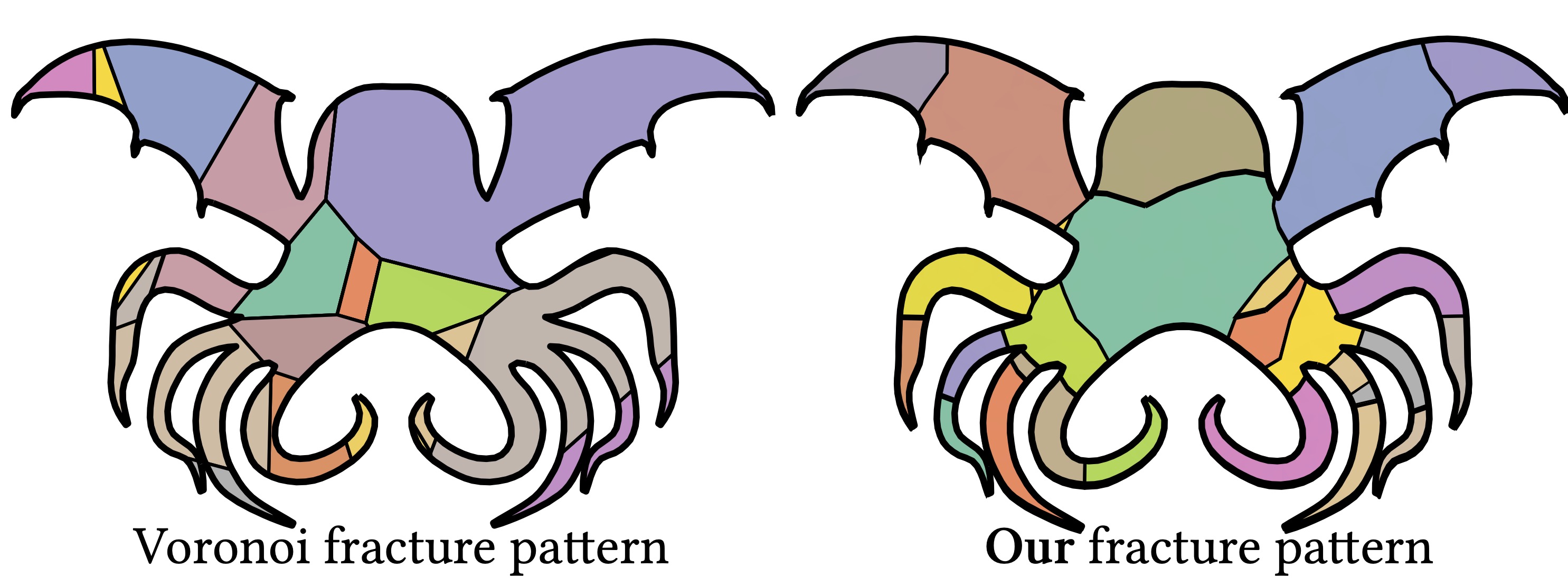
Figure 2. Popular Voronoi-based prefracturing results in recognizable, unrealistic shapes. Our fracture modes break across weak regions.

The first $k$ fracture modes can be intersected against each other to define a prefracture pattern as a drop-in replacement to existing procedural methods (see Fig. 2). Furthermore, impacts determined at runtime can be efficiently projected onto the linear space of precomputed fracture modes to obtain impact-dependent fracture without the need for costly stress computation or crack propagation.

We demonstrate the theoretical and practical advantages and limitations of our algorithm over existing procedural methods and evaluate its accuracy by qualitatively comparing to existing works in worst-case structural analysis. We showcase the benefits of our algorithm within an off-the-shelf rigid body simulator to produce animations on a diverse set of shapes and impacts. We show the realtime potential of fracture modes with a prototypical interactive 2D application (see Fig. 4 and accompanying video).

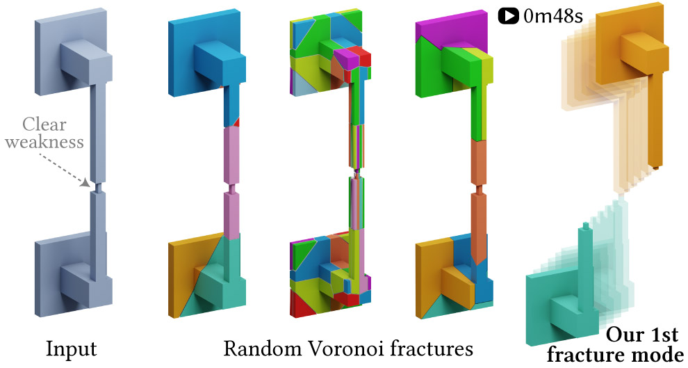
Figure 3. Existing procedural prefracture algorithms (center) rely on randomness and do not account for the geometrically weak regions of an object, unlike our proposed fracture modes (right).

2. Related Work

Fracture simulation has an extensive body of previous work; Muguercia et al. [2014] provide a thorough survey. Stiff brittle fracture is characterized when little or no perceptible deformation occurs before fracture (i.e., when the object is otherwise rigid). Modeling the dynamic or quasistatic growth of brittle fracture patterns in a high performant way requires not just high spatial resolution but also high temporal resolution at the microsecond scale [Kirugulige et al., 2007], modeling stress concentration and subsequent release. This process has been approximated, for example, using mass-springs [Norton et al., 1991; Hirota et al., 1998], finite elements [O’Brien and Hodgins, 1999; Kaufmann et al., 2009; Wicke et al., 2010; Pfaff et al., 2014; Koschier et al., 2015], boundary elements [Zhu et al., 2015; Hahn and Wojtan, 2015, 2016], and the material-point method [Wolper et al., 2019; Wolper et al., 2020; Fan et al., 2022]. While any such method can eventually meet realtime demands by lowering the discretization fidelity (e.g., on low-res cage geometry [Parker and O’Brien, 2009; Muller et al., 2004] or a modal subspace [Glondu et al., 2012]) or assuming large enough computational resources, we instead focus our attention to previous methods which achieve realtime performance via the well established workflow of prefracturing. This workflow sidesteps computationally expensive and numerically fragile remeshing operations. It fits tidily into the existing realtime graphics pipeline, where geometric resolutions and computational resources can be preallocated to ensure low latency and consistent performance.

Creating prefracture patterns manually requires skill and time, precluding fully automatic pipelines. Many commercial packages (e.g., Unreal Engine, Houdini) implement or suggest geometric prefracturing heuristics to segment a shape into solid subfragments. Voronoi diagrams of randomly scattered points [Raghavachary, 2002; Oh et al., 2012] capture the stochastic quality of fracture, but result in overly regular and convex fragments with perfectly flat sides. Despite lacking realism, convexity can be advantageous for simulations. For example, it enables realtime collision detection and even offline at massive scales [Zafar et al., 2010]. Beyond collision detection, approximate convex decomposition has been employed as a prefracturing technique, allowing fracture patterns to be applied locally at low cost [Müller et al., 2013]. Müller et al. [2013] rely on manual intervention at multiple stages, making it not comparable as an automatic method; however, we compare to the Voronoi decomposition it is based on in Figs. 2 and 3.

Schvartzman and Otaduy [2014] increase the space of possible fragments beyond convexity by computing the Voronoi decomposition on a higher dimensional embedding. The regularity of these fragments can be augmented further by randomly generated “cutter” objects (i.e., bumpy planes slicing though the input shape) or perturbed level set functions (see, e.g., [Museth et al., 2021]). These stochastic methods often miss obvious structural weaknesses (see Fig. 3) or result in implausible fragments (see Fig. 5). While the defects of these methods can be resolved manually, hidden behind destruction dust or obscured by fast explosions, our fracture modes consistently produce non-convex fragments whose boundaries originate from minimal stress displacements of the shape. Beyond taking into account the physical elastic behavior of the geometry, our method can incorporate constraints to avoid fractures in certain areas. While our fracture modes are slower to compute than geometric-only procedural prefracture, this cost is added only at the offline precomputation stage.

Given a precomputed fracture pattern, one must decide which fractures are activated when the object receives a given online impact. Strategies range from simple heuristics like Euclidean distance thresholds and centering a spatial fracture pattern on the contact point [Müller et al., 2013; Su et al., 2009] to learning from examples [Schvartzman and Otaduy, 2014]. A key practical contribution of our fracture modes is that they span a linear subspace onto which impacts can be cheaply projected to trigger fragment displacements at runtime, removing the need for heuristics or data-based approaches.

Figure 4. Screenshots of our 2D interactive prototype, in which the user can select the impact position to obtain different breaking patterns.

2.1. Sparsified eigenproblems

Our approach for defining fracture modes lies within a broader class of optimization problems of the form:

(1) $$\mathop{\text{argmin}}_{\mathbf{X}^{\top}\mathbf{M}\mathbf{X}=\mathbf{I}}\quad\frac{1}{2}\mathop{\text{trace}}\left(\mathbf{X}^{\top}\mathbf{L}\mathbf{X}\right)+\sum_{i=1}^{k}g(\mathbf{X}_{i})\,,$$

where $\mathbf{X}_{i}$ as the $i^{\text{th}}$ column of $\mathbf{X}∈ℝ^{n×k}$ is referred to as a modal vector or mode, $\mathbf{M}$ and $\mathbf{L}$ are positive semi-definite $n×n$ matrices, and $g:ℝ^{n}\textrightarrow ℝ$ is a sparsity-inducing norm, like $g(\mathbf{x})=\|\mathbf{x}\|_{1}$. When $g\coloneqq 0$, this reduces to the generalized eigenvalue problem (see e.g., [Bai et al., 2000] Chaps. 4-5), whose solution satisfies $\mathbf{L}\mathbf{X}=\mathbf{M}\mathbf{X}Λ$, where the diagonal $k×k$ matrix $Λ$ contains the $k$ smallest eigenvalues ($Λ_{i,i}=\mathbf{X}_{i}ᵀ\mathbf{L}\mathbf{X}_{i}$). For non-trivial $g$, we may continue to consider $λ_{i}=\mathbf{X}_{i}ᵀL\mathbf{X}_{i}+g(\mathbf{X}_{i})$ as describing the frequency of the $i^{\text{th}}$ mode.

Ozolins et al. [2013] proposed the notion of compressed modes using a sparsity-inducing $\ell_{1}$-norm to compute localized (sparse) solutions to Schrödinger’s equation. Neumann et al. [2014] extended this idea to compressed eigenfunctions of the Laplace-Beltrami operator on 3D surfaces, advocating for an alternating direction method of multipliers (ADMM) optimization method. While ADMM’s standard convergence guarantees [Boyd, 2010] do not apply to non-convex problem such as Eq. (1), Neumann et al. [2014] demonstrate successful local convergence albeit with dependency on the initial guess and optimization path. Replacing the $\mathbf{X}^{\top}\mathbf{L}\mathbf{X}$ term with a data-term, Neumann et al. [2013] use a similar ADMM approach to create sparse PCA bases for mesh deformations.

Brandt and Hildebrandt [2017] further extend this line of smooth, sparse modal decompositions by considering $L$ to be the Hessian of an elastic energy. They propose an iterative mode-by-mode optimization. The current mode is optimized by sub-iterations consisting of a quadratic program solve resulting from linearizing the constraints around the current iterant interleaved with normalization in order to approach a unit-norm vector. Despite the conspicuous downside that any sub-optimality of earlier modes is locked in possibly affecting the accuracy of later modes, this method enjoys performance and robustness improvements over the ADMM approach of Neumann et al. [2014]. Therefore, we follow suit with a similarly mode-by-mode fixed-point iteration approach. Unique to our method is that we do not consider the sparsity of the modal vector itself, but rather the sparsity of the mode’s continuity over the domain.

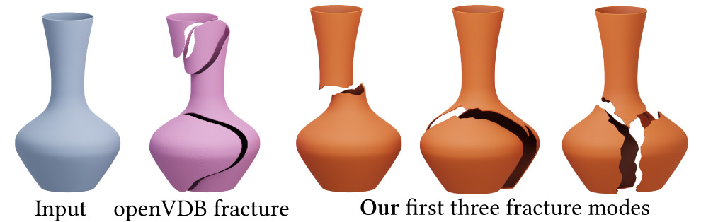
Figure 5. Level-set methods (e.g., OpenVDB [Museth et al., 2021]) will produce non-convex, yet implausible fracture patterns unrelated to the structural integrity of the shape.

3. Fracture Modes

Given an elastic solid object $\Omega\subset\mathbb{R}^{d}$ and a deformation map ${u:\Omega\to\mathbb{R}^{d}}$, we can formulate the object’s total strain energy as

(2) $$E_{\Psi}(u)=\int_{\Omega}\Psi(u,x)dx,$$

where $\Psi$ is the strain energy density function evaluated at points $x\in\Omega$ in the undeformed object.

Suppose we allow the deformation map $u$ to fracture the object $\Omega$ into two disjoint pieces $\Omega_{1}$ and $\Omega_{2}$ along a given $(d-1)$-dimensional fracture fault $S$ (see inset). Effectively, we’re allowing $u$ to be discontinuous at $S$. Consider $x_{1}$ and $x_{2}$ to be the undeformed positions of points infinitesimally on either side of a point $x∈S$ on the fracture fault. Then, the difference between $u(x_{1})$ and $u(x_{2})$ describes the pointwise vector-valued discontinuity at $x\in S$:

(3) $$D(u,x∈S)=u(x_{1})-u(x_{2})\in\mathbb{R}^{d},$$

where $D=\mathbf{0}$ would indicate continuity or absence of fracture. We can then compute the discontinuity energy associated with $S$ as

(4) $$\int_{x\in S}\|D(u,x)\|^{2}dx\,,$$

which can be seen as a cohesive surface energy from the FEM crack propagation literature (e.g., [Ortiz and Pandolfi, 1999]). Unlike similar cohesive energies found in graphics (e.g., for UV mapping [Poranne et al., 2017] or shape interpolation [Zhu et al., 2017]), assuming small displacements affords us this simpler, first-order approximation.

We now consider that the set of admissible discontinuities is not just a single fracture fault, but a finite number of fault patches: $S=\{S_{1},…,S_{p}\}$. We assume that $S$ comes from a, for now, arbitrary over-segmentation of $Ω$. This could be created with a high-resolution Voronoi diagram, by intersecting $Ω$ with random surfaces, voxel boundaries, or by some a priori distribution of granular subobjects. We define the total discontinuity energy associated with $u$ as

(5) $$E_{D}(u)=\|D(u,S)\|_{2,1} \coloneqq\sum_{i=1}^{p}\sqrt{\int_{S_{i}}\|D(u,x)\|^{2}dx}.$$

We add this to the strain energy to form the total energy:

(6) $$E(u)=E_{\Psi}(u)+\omega\,E_{D}(u),$$

where $\omega∈ℝ$ is a positive weight balancing the two terms. In the cohesive FEM context, $\omega$ can be understood as the square root of the traction-displacement coefficient in the first fracture phase [Chowdhury and Narasimhan, 2000]. Minimizing the $\ell_{2,1}$ norm on the matrix $D$ is tantamount to minimizing the sparsity-inducing [Candes and Wakin, 2008] $\ell_{1}$ norm on the lengths of each row. Minimizing the $\ell_{1}$ norm ($\sum_{i}\sum_{j}|D_{ij}|$) directly would also lead to sparsity, but the solution would be rotationally dependent.

Figure 6. Zhou et al. [2013] (left) identify the geometrically weakest regions of a given shape, which align with their real-world experiments (center). Our fracture modes (right) produce fracture patterns qualitatively similar.

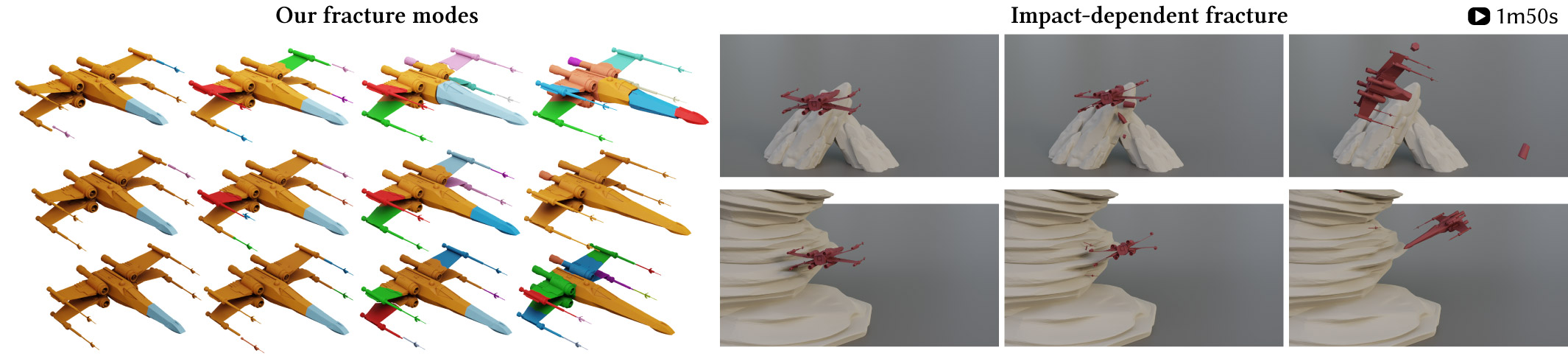
Figure 7. The same prefractured modes can be used to simulate many different impacts; for example, a racing simulator may destroy the player’s spaceship differently depending on its impact.

We can now define the $k$ lowest energy fracture modes as the set of mass-orthonormal deformation maps $\{u^{i}\}_{i=1}^{k}$ that minimize their combined total energy; i.e.,

(7) $$\{u^{i}\}_{i=1}^{k}=\mathop{\text{argmin}}_{\{u^{i}\}_{i=1}^{k}}\sum\limits_{i=1}^{k}E(u^{i})\,,\qquad\text{s.t.}\quad\int_{\Omega}(u^{i})^{\top}\rho u^{j}dx=\delta^{i,j},$$

where $\rho$ is the local mass density and $\delta^{i,j}$ is the Kronecker delta. In general, for large enough $ω$, minimizers $u^{i}$ will have exactly zero $E_{D}$ on all but a sparse subset of fault patches in $S$, agreeing with the usual sparse coding theory [Candes and Wakin, 2008].

3.1. Fracture Modes on Meshes

We will derive a discrete formulation of the variational problem in Eq. (7) for a 2D solid object, represented as a triangle mesh $\Omega$ with $n$ vertices and $m$ faces. In this construction, the mesh’s $p$ interior edges will correspond to admissible fracture faults $S_{1},\cdots,S_{p}$. Everything that follows is straightforward to extend to 3D solids by exchanging triangles and interior edges for tetrahedra and interior faces.

A traditional piecewise-linear finite element method (FEM) would discretize the strain energy $E_{\Psi}$ using hat functions $\varphi_{i}:\Omega\rightarrow\mathbb{R},$ $\forall i=1,\dots,n$ and associate a scalar function $u:\Omega\rightarrow\mathbb{R}$ with a vector $\mathbf{u}\in\mathbb{R}^{n}$ such that

(8) $$u(x)=\sum_{i=1}^{n}\mathbf{u}_{i}\varphi_{i}(x).$$

Vector-valued $u:\Omega\rightarrow\mathbb{R}^{d}$ such as a deformation would be described coordinate-wise in the same way, via a vector $\mathbf{u}\in\mathbb{R}^{dn}$.

Hat functions are by construction continuous. Normally, this is a good thing, but we would like to have functions with arbitrarily large co-dimension one patches of discontinuities. Let us introduce the concept of an exploded mesh $\tilde{\Omega}$, with the same $m$ faces as $\Omega$ and same carrying geometry, but where each vertex is effectively repeated for each incident triangle. Thus, $\tilde{\Omega}$ is composed of $m$ combinatorially disconnected triangles and $3m$ vertices $v_{cf}$ with $c=1,2,3$ and $f=1,\dots,m$.

Hat functions $\tilde{\varphi}:\tilde{\Omega}\rightarrow\mathbb{R}$ defined on $\tilde{\Omega}$ reduce to barycentric coordinate functions extended with zero value outside the corresponding triangle (see inset). These trivially span the space of piecewise linear scalar discontinuous functions $u$ via vectors $\mathbf{u}\in\mathbb{R}^{3m}$:

(9) $$u(x)=\sum_{f=1}^{m}\sum_{c=1}^{3}\mathbf{u}_{cf}\tilde{\varphi}_{cf}(x).$$

We will use this basis for each coordinate of our vector-valued deformation map, captured in a vector of coefficients $\mathbf{u}\in\mathbb{R}^{(d+1)md}$, with the displacement at vertex $c$ of face $f$ selected by $\mathbf{u}_{cf}\in\mathbb{R}^{d}$.

We may now discretize both terms in our energy in Eq. (6). First, the integral strain energy follows the usual FEM discretization as a sum over each element.

(10) $$E_{\Psi}(\mathbf{u})=\sum_{f=1}^{m}\int_{f}\Psi(u,x)dx\,.$$

We can abstract the choice of $\Psi$ for now by considering small displacements around the rest configuration such that it can be approximated by its Hessian matrix $\mathbf{Q}∈ℝ^{(d+1)md×(d+1)md}$:

(11) $$E_{\Psi}(\mathbf{u})\approx\frac{1}{2}\mathbf{u}^{\top}\mathbf{Q}\mathbf{u}\,.$$

In Section 3.7 we discuss a further approximation specific to our model. Our basis functions $\tilde{\varphi}$ will only allow fractures along the mesh’s interior edges, therefore, the integral in Eq. (5) breaks into a contribution from each interior edge $e$:

(12) $$E_{e}(u)=\sqrt{\int_{e}\|D(u,x)\|^{2}dx}\,,$$

which we can compute exactly by two-point Gaussian quadrature (the integrand is a second-order polynomial).

For a given edge $e$ with length $l$, corresponding to vertex pairs $\{af,bf\}$ and $\{cg,dg\}$ (see inset), this amounts to

$$E_{e}(\mathbf{u}) =\sqrt{\frac{l}{2}\left(\left\|\mathbf{d}\left(\tfrac{+1}{\sqrt{3}}\right)\right\|_{2}^{2}+\left\|\mathbf{d}\left(\tfrac{-1}{\sqrt{3}}\right)\right\|_{2}^{2}\right)}\quad\quad\quad\quad\quad\quad\quad\quad$$

where

(13) $$\mathbf{d}(t) =\frac{1+t}{2}(\mathbf{u}_{af}-\mathbf{u}_{cg})+\frac{1-t}{2}(\mathbf{u}_{bf}-\mathbf{u}_{dg})$$

measures the pointwise discontinuity for the quadrature at parametric location $t∈[-1,1]$ along the edge.

The full discontinuity energy associated with the map $u(x)$ is given by summing over every interior edge

(14) $$E_{D}(\mathbf{u})=\sum_{e=1}^{p}E_{e}(\mathbf{u})\,.$$

Finally, we can define the $k$ lowest-energy discrete fracture modes as column vectors of a matrix $\mathbf{U}∈ℝ^{(d+1)md×k}$ satisfying

(15) $$\mathop{\text{argmin}}_{\mathbf{U}^{\top}\tilde{\mathbf{M}}\mathbf{U}=\mathbf{I}}\quad\frac{1}{2}\mathop{\text{trace}}\left(\mathbf{U}^{\top}\mathbf{Q}\mathbf{U}\right)+\omega\sum_{i=1}^{k}\left(E_{D}(\mathbf{U}_{i})\right),$$

where $\tilde{\mathbf{M}}$ is the possibly lumped FEM mass matrix defined on the exploded mesh $\tilde{\Omega}$.

3.2. Optimization

The definition of fracture modes on meshes involves solving the optimization problem in Eq. (15). While the objective term is convex, the orthogonality constraints are not. To proceed, we adapt the Iterated Convexification for Compressed Modes (ICCM) scheme proposed by Brandt and Hildebrandt [2017]. ICCM computes the modes sequentially, assuming the first $i-1$ columns of $\mathbf{U}$ have been computed. In the original ICCM formulation, the process for finding the $i^{\text{th}}$ column, $\mathbf{U}_{i}$ proceeds by choosing a random unit-norm vector $\mathbf{c}$, then repeatedly solving

(16) $$\mathbf{U}_{i}\leftarrow \mathop{\text{argmin}}_{\mathbf{u}}\frac{1}{2}\mathbf{u}^{\top}\mathbf{Q}\mathbf{u}+\ \omega\ E_{D}(\mathbf{u})$$

(17) $$\text{subject to}\ \begin{bmatrix}\mathbf{U}_{1}^{\top}\\ \vdots\\ \mathbf{U}_{i-1}^{\top}\\ \mathbf{c}^{\top}\end{bmatrix}\tilde{\mathbf{M}}\mathbf{u}=\begin{bmatrix}0\\ \vdots\\ 0\\ 1\end{bmatrix}$$

and updating

(18) $$\mathbf{c}\leftarrow \frac{\mathbf{U}_{i}}{\sqrt{\mathbf{U}_{i}^{\top}\tilde{\mathbf{M}}\mathbf{U}_{i}}},$$

until convergence is detected by $\|\mathbf{U}_{i}-\mathbf{c}\|$ falling below some tolerance $\varepsilon$. By linearizing the (quadratic) norm constraint, the minimization problem Eq. (16) is a convex conic problem and solved with off-the-shelf techniques (see Appendix A).

We found that random initializations for $\mathbf{c}$ not only introduce non-determinism, but can also sometimes result in a large number of inner iterations and sub-optimal local minima (see Fig. 8). Instead, when computing $\mathbf{U}_{i}$ we initialize $\mathbf{c}$ with the $i^{\text{th}}$ continuous eigenvectors of $\mathbf{Q}$ (defined on the unexploded mesh). We compute these $k$ initial vectors at once using the SciPy wrapper for the sparse eigen solver Arpack [Lehoucq et al., 1998]. We outline our complete fracture mode computation algorithm in Algorithm 1.

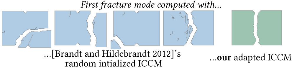
Figure 8. We adapt the algorithm suggested by Brandt and Hildebrandt [2017] to use the eigenmodes of $\mathbf{Q}$ as initial guesses as opposed to random vectors.

3.3. Impact-dependent fracture

By construction, the columns of $\mathbf{U}$ form an orthonormal basis of the lowest-energy $k$-dimensional subspace of possible fractures of $\Omega$. This key feature means we can precompute an object’s fracture modes right after its design. Then, inside an interactive application we can project any detected impact onto our modes to obtain impact-dependent realtime fracture (see Fig. 9).

If a collision is detected between $\Omega$ and another object, with contact point $p$ and normal $\vec{n}$, we can define the exploded-vertex-wise impact vector $\mathbf{w}∈ℝ^{(d+1)md}$. Ideally, $\mathbf{w}$ would be the displacements determined by an extremely short-time-duration simulation of elastic shock propagation. In lieu of being able to compute this in realtime, we use an approximation based on distance to smear the impact into the object:

(19) $$\mathbf{w}_{cf}=g(p,v_{cf})\,\vec{n}\,,\quad\forall c=1,2,3\,,\,f=1,\dots,m$$

where $g$ is a filter that vanishes as $v_{cf}$ is far from $p$. Then, we project $\mathbf{w}$ onto our modes to obtain our projected impact

(20) $$\mathbf{w}^{\star}=\sum_{i=1}^{k}\mathbf{U}_{i}\mathbf{U}_{i}^{\top}\tilde{\mathbf{M}}\mathbf{w}=\sum_{i=1}^{k}\mathbf{U}_{i}\mathbf{U}_{i}^{\top}\tilde{\mathbf{M}}\mathbf{g}\vec{n}$$

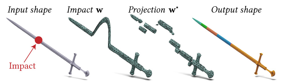
Figure 9. We propagate any impact (left) using an elastic shockwave (middle). We then project this propagated impact onto our modes (right). At runtime (see text), we compute $\mathbf{w}^{\star}$ directly without the need for linear solves.

Figure 10. A larger threshold (smaller impact) produces less fracture pieces.

An immediate choice of $g$ would be a Gaussian density function centered at $p$. A more physically based choice of $g$ can be obtained through a single implicit timestep of an elastic shockwave equation

(21) $$\mathbf{g}=\left(\tilde{\mathbf{M}}-\tau\tilde{\mathbf{L}}\right)^{-1}\tilde{\mathbf{M}}\delta_{p}\,,$$

where $\tau$ is the timestep of the simulation our fractures are embedded in. This choice of $g$ has benefits beyond physical inspiration, by ensuring an impact is only blurred onto regions that are geodesically close to one another, regardless of whether they are Euclideanly close (see Fig. 9). However, computing this $\mathbf{g}$ upon impact would involve solving a linear system at runtime. We avoid this by precomputing

(22) $$\mathbf{A}_{i}=\mathbf{U}_{i}^{\top}\tilde{\mathbf{M}}\left(\tilde{\mathbf{M}}-\tau\tilde{\mathbf{L}}\right)^{-1}\tilde{\mathbf{M}}\,,$$

thus requiring only a matrix multiplication at runtime:

(23) $$\mathbf{w}^{\star}=\sum_{i=1}^{k}\mathbf{U}_{i}\mathbf{A}_{i}\delta_{p}\vec{n}\,.$$

Let $\tilde{\Omega}_{\mathbf{w}^{\star}}$ be the exploded mesh $\tilde{\Omega}$ as deformed by the map $w^{\star}$. For any two vertices $v_{af},v_{cg}$ that are coincident in $\tilde{\Omega}$ (i.e., that came from the same original vertex in $\Omega$), we will glue (i.e., un-explode) them if their deformation maps differ by less than some tolerance, $\|\mathbf{w}^{\star}_{af}-\mathbf{w}^{\star}_{cg}\|<\sigma$. This results in a new fractured mesh $\Omega^{\star}$, whose fracture pattern depends meaningfully on the nature of the impact and which we can output to the simulation.

Our single timestep in Eq. (21) is an approximation that makes $\mathbf{w}^{\star}$ depend linearly on the impact. This has the added effect that scaling $\sigma$ and scaling the magnitude of the impact are equivalent in our model. Thus, $\sigma$ could be linked to the force of the impact or the relative speed if one has access to this dynamic information (see Fig. 10). We note that this equivalence is a product of our modeling choices and may not always yield physically accurate results. For example, a large force on a small area may cause immediate local fractures, quickly reducing the stress before it propagates further; in our model, the same impact would likely cause large global fractures.

Let $\mathbf{Q}$ be a PSD matrix, $k\in\mathbb{N}$

$\mathbf{C}\leftarrow\text{eigenvectors}(\mathbf{Q},\mathbf{M},k)$

for $i=1,\dots,k$ do

       $\mathbf{c}\leftarrow\mathbf{C}_{i}$

       repeat

             $\mathbf{U}_{i}\leftarrow$ solve Eq. (16) (see Appendix A)

             $\mathbf{c}\leftarrow\mathbf{U}_{i}/\sqrt{\mathbf{U}_{i}^{\top}\tilde{\mathbf{M}}\mathbf{U}_{i}}$

            

      until $\|\mathbf{U}_{i}-\mathbf{c}\|\leq\varepsilon$

return $\mathbf{U}$

Algorithm 1 Fracture Modes via Adapted ICCM

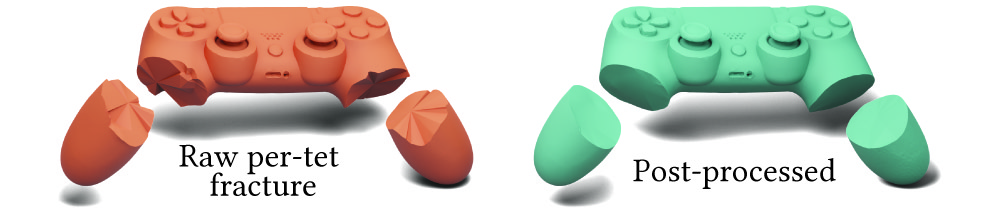
Figure 11. We use the upper envelope extraction algorithm by Abdrashitov et al. [2021] to obtain smoothed fracture faults.

3.4. Efficient implementation for real-time fracture

In 3D, our fracture mode computation needs a tetrahedralization of the input’s interior, but practical realtime applications prefer to work with triangle surface meshes for input and output. Fortunately, the sparsity inducing discontinuity norm results in fracture modes which are continuous across most pairs of neighboring tetrahedra. It is unnecessary to keep the entire tetrahedral mesh at runtime. Instead, we can determine the connected components determined by neighboring tetrahedra whose shared face’s discontinuity term is below $\sigma$ across all $k$ modes (or below the lowest possible $\sigma$ allowed by the dynamic system). The boundary of each component is a solid [Zhou et al., 2016] triangle mesh of a fracture fragment. Since the impact projection described above is linear, we can pre-restrict the projection to vertices on the boundary of these fragments, discarding all internal vertices and the tetrahedral connectivity.

3.5. Simple Nested Cages

In practice, the input model may be very high-resolution, not yet fully modeled when fractures are precomputed, or too messy to easily tetrahedralize. Like many simulation methods before us, we can avoid these potential performance, workflow and robustness problems by working with a tetrahedralization coarse cage nesting the input model. The Nested Cages method of Sacht et al. [2015] produces tight fitting cages, but suffers long runtimes, potential failure, and may result in a surface mesh which causes subsequent tetrahedralization (e.g., using TetWild [Hu et al., 2018] or TetGen [Si, 2015]) to fail.

Therefore, in Algorithm 2 we introduce a very simple caging method inspired by the level-set method of Ben-Chen et al. [2009]. As an example, Nested Cages crashes after a minute on the input mesh in the inset, while our simple algorithm produces a satisfying output cage after 85 seconds.

Let $V_{\text{in}},F_{\text{in}}$ be the vertex and face lists of the input mesh, and

$m_{\text{target}}$ the desired number of output faces.

Binary Search on offset amount $d$

       $V_{\text{mc}}$,$F_{\text{mc}}\leftarrow$ marching-cubes( distance to $V_{\text{in}}$,$F_{\text{in}}$ minus $d$)

       $V_{\text{d}}$,$F_{\text{d}}\leftarrow$ decimate $V_{\text{mc}}$,$F_{\text{mc}}$ to $m$ faces

       $V_{\text{u}}$,$F_{\text{u}}\leftarrow$ self-union $V_{\text{d}}$,$F_{\text{d}}$ via [Zhou et al., 2016]

       $V_{\text{t}}$,$T_{\text{t}},F_{\text{t}}\leftarrow$ tetrahedralize $V_{\text{u}}$,$F_{\text{u}}$ via [Si, 2015]

       if any step failed or $V_{\text{t}}$,$F_{\text{t}}$ does not strictly contain $V_{\text{in}}$,$F_{\text{in}}$  then

            increase $d$

      else

            decrease $d$

      

return $V_{\text{t}}$,$T_{\text{t}}$

Algorithm 2 Simple nested cages via binary search

Like Nested Cages, the output cage will strictly contain the input, but also by construction we ensure that this cage can be successfully tetrahedralized (not just in theory). In a sense, this method provides a different point on the Pareto frontier of tightness-vs-utility. Each step is a fairly standard geometry processing subroutine with predictable performance, and one may even consider using it as an initialization strategy for Nested Cages to improve tightness in the future. We run a max of 10 search iterations, lasting between 5 and 20 seconds each in our examples.

Fracture modes and solid fragment components on the cage’s tetrahedralization can be transferred to the true input geometry by intersecting each connected component against the input mesh. In this way, the exterior surface of each fragment component is exactly a subset of the input mesh.

3.6. Smoothing internal surfaces

By our construction, the fracture boundaries will follow faces of the tetrahedral mesh used for their computation. This reveals aliasing with frequency proportional to the mesh resolution. We may optionally alleviate this by treating each extracted per-tet component membership as a one-hot vector field, which we immediately average onto (unexploded) mesh vertices stored as a matrix $\mathbf{Z}∈[0,1]^{n×|\text{components}|}$, so that $\mathbf{Z}_{i,j}∈[0,1]$ is viewed as the likelihood that vertex $i$ belongs to component $j$. We apply implicit Laplacian smoothing with a time step of $λ$ to columns of $\mathbf{Z}$:

(24) $$\mathbf{Z}\leftarrow(\mathbf{M}+λ\mathbf{L})^{-1}(\mathbf{M}\mathbf{Z}),$$

where $\mathbf{M}$, $\mathbf{L}$, are the mass and Laplacian matrices, respectively. The resulting $\mathbf{Z}$ continue to contain fractional values in $[0,1]$ corresponding to a smoothed likelihood. We now re-extract piecewise-linear (triangle mesh) component boundaries by computing the upper-envelope (tracking the argmax) using the implementation of Abdrashitov et al. [2021]. While essentially still using the same tetrahedral mesh, utilizing smoothing and piecewise-linear interpolation greatly reduces aliasing artifacts (see Fig. 11).

By the nature of the Laplacian, Eq. (24) will push our fracture faults towards smooth surfaces. This is in alignment with our modeling decisions at the beginning of Section 3: as our set of possible fault patches $S_{i}$ becomes larger, the area integral in Eq. (5) will encourage smoother fracture fault surfaces. Thus, the postprocessing described here is not a departure from our model; rather, a way of alleviating the error introduced by the mesh discretization.

In the real world, crystalline materials do break along smooth surfaces aligned with their internal structure in a phenomenon known as cleavage (see e.g., [Ford and Dana, 1922] Part II.I.277). On the other hand, materials like wood or clay do not necessarily break along smooth faults like those produced by our method. This is a well-studied limitation we share with all mesh-based fracture algorithms and which could be alleviated by borrowing strategies from the literature like the Adaptive Fracture Refinement by Chen et al. [2014], perturbation of crack surface vertices as described by Fan et al. [2022], or the use of pre-authored “splinters” suggested by Parker and O’Brien [2009].

3.7. Choice of strain energy

So far the only requirement on the strain energy density $\Psi$ is that we can construct its second-order approximation near the rest configuration represented by the (positive semi-definite) Hessian matrix $\mathbf{Q}$. We now investigate the effect of choices of $\mathbf{Q}$ and in particular the relationship with the balancing weight $\omega$.

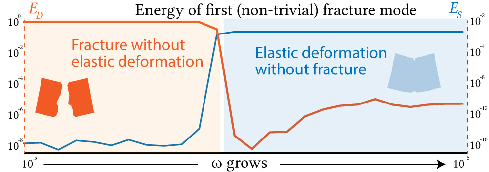
Figure 12. As our energy weight changes, our output modes sharply transition from only deforming to only fracturing. This gives us the additional insight that fractures occur only within the nullspace of the strain energy, and has the additional effect of making $\omega$ a simple parameter to set.

To make our investigation concrete, take $\Psi$ to be the linear elastic strain energy density, so that $\mathbf{Q}$ is the common linear elasticity stiffness matrix. Our observations also follow if one chooses $\mathbf{Q}$ to be the Hessian of other, nonlinear energies like the Neohookean or St. Venant-Kirchhoff ones. By sweeping across values of $\omega$ we see a sharp change in the first (and all) fracture mode’s behavior with the discontinuity energy dominating over the strain energy and then sharply swapping (see Fig. 12). When the discontinuity energy is effectively zero, then we have simply recovered the usual linear elastic vibration modes (albeit in a convoluted way).

When the strain energy is effectively zero, then we not only start to see sparse fractures, but we also see that each fracture fragment undergoes its own zero-strain energy transformation. This behaviour is consistent even in larger order modes (inset). That is, each fragment undergoes a linearized rigid transformation, the only motions in the null space of the strain energy. Physically, this behaviour naturally aligns our fracture modes with the traditional definition of stiff brittle fracture, where materials do not significantly deform before breaking. This is also interesting from a numerical perspective as it implies that the precise choice $\mathbf{Q}$ is irrelevant and only its null space matters.

Table 1. Performance details for all our examples

Fig.	#T	Time/mode (s)	$k$	$p$	Impact Proj. (ms)
7	6316	2.86	30	47	1.06
18	3931	2.20	20	117	1.21
14 (a)	3545	0.63	10	35	1.13
14 (b)	4993	2.63	25	34	1.08
16	12162	11.6	10	31	1.19
19	8802	5.91	15	152	1.96

With this in mind, we consider whether all linearized rigid transformations should be admissible. Since we ultimately care about the fracture pattern created by the modes, we observed qualitatively that the scaling induced by linearized rotations resulted in small elements breaking off and expanding between fragment boundaries to reduce the discontinuity energy. Rather than attempt to identify these as outliers, we found a simpler solution is to work with a strain energy that only admits translational motions in its null space, namely, $\Psi(u,x)=\|\nabla u(x)\|^{2}$. The Hessian of $\|\nabla u(x)\|^{2}$ is simply the cotangent Laplacian matrix $\tilde{\mathbf{L}}∈\mathbb{R}^{(d+1)m×(d+1)m}$ repeated for each spatial coordinate:

(25) $$\mathbf{Q}=\mathbf{I}_{d}\otimes\tilde{\mathbf{L}}.$$

This choice of $\mathbf{Q}$ is used in all our examples.

Efficient precomputation

Our observation regarding the nullspace of $\mathbf{Q}$ can be further exploited to greatly reduce the cost of our offline mode precomputation step. Our strain energy being numerically zero in all our modes means all (exploded) vertices belonging to a single element undergo identical deformations. Therefore, by transforming this observation into an assumption, we may store deformations solely at elements, reducing our number of variables by a factor of $d+1$. This ensures that the strain energy measure on the exploded mesh will always be null, which also means we can remove the quadratic term $\mathbf{u}^{\top}\mathbf{Q}\mathbf{u}$ from Eq. (16). Further, allowing only per-element deformations also makes our vector discontinuity $D$ necessarily constant along element boundaries, which makes its integral in Eq. (13) trivial without the need of quadrature nodes. The combination of all these observations significantly reduce the size of our conic problem (see Appendix B), allowing computation of identical fracture modes several orders of magnitude faster.

Figure 13. Our precomputed fracture modes identify the geometrically weakest regions of a shape, and are activated or not on runtime depending on the nature of the impact.

4. Timing & Implementation details

We have implemented our main prototype in Python, using Libigl [Jacobson et al., 2018]. We used Mosek [ApS, 2019] to solve the conic problem in Eq. (16). We report timings conducted on a 2020 13-inch MacBook Pro with 16 GB memory and 2.3 GHz Quad-Core Intel Core i7 processor. To produce our animations, we follow a traditional Houdini [SideFX, 2020] fracture simulation workflow, exchanging the usual Voronoi or openVDB fracture nodes for our own fractured meshes. Our impact projection step could be fully integrated into Houdini’s rigid body simulator at a minimal performance cost. Only for simplicity in prototyping, we chose not to do this and instead compute our final mesh $\Omega^{\star}$ in Python taking into account the animation’s impact and load it into Houdini directly to show a prototype of what our algorithm would look like integrated in a rigid body simulation.

Our algorithm’s only parameters are the tolerances $\varepsilon$ and $\sigma$, which we fix at $\varepsilon=10^{-10}$ and $\sigma=10^{-3}$. As we discuss in Section 3.7, a scalar $\omega$ will not actually have an effect in the output as long as it is small enough for us to be within the zero-deformation fracture realm (see Fig. 12).

Our proposed algorithm works in two steps. First, we precompute a given shape’s fracture modes. This step takes place offline, following Algorithm 1. The computational bottleneck of this section of our algorithm is the conic solve detailed in Eq. (16). Each mode takes between 0.5 and 12 seconds to compute in our meshes, which have between 3,000 and 15,000 tetrahedra.

Secondly, our impact projection step as detailed in Section 3.3 is the only part of our algorithm that happens at runtime. The complexity of this step is dominated by the projection step in Eq. (20), which is $\mathcal{O}(k\tilde{n})$, where $k$ is the number of precomputed modes and $\tilde{n}$ is the number of vertices in the boundary of the connected components described in Section 3.4. All other elements of our projection step are $\mathcal{O}(p)$, where $p$ is the number of connected components (in our example between 10 and 500) and $p<<n$ so they can be disregarded from the complexity discussion. In our examples, $\tilde{n}$ is between 1,000 and 10,000 and we compute between $k=20$ and $k=40$ fracture modes, meaning our full runtime step requires between $0.1$ and $1$ million floating point operations, putting it well within realtime requirements, even if one greatly increases $\tilde{n}$, $k$ or the number of objects on scene (note this projection step only needs to be run when a collision is detected, and not at every simulation frame). Our unoptimized, CPU implementation takes between one and two miliseconds to carry out this step on our laptop (see Table 1).

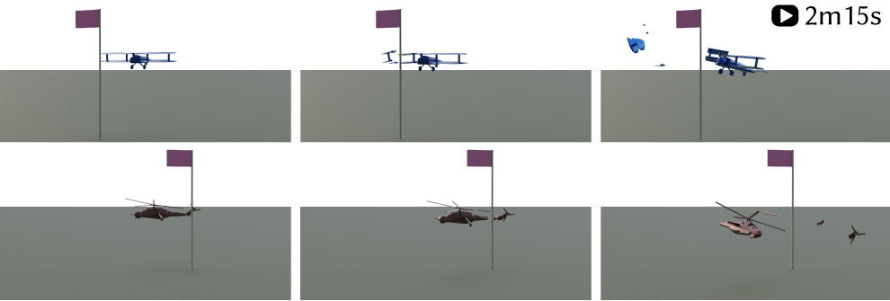
Figure 14. Similar impacts result in different fracture patterns once we have computed our fracture modes for different objects.

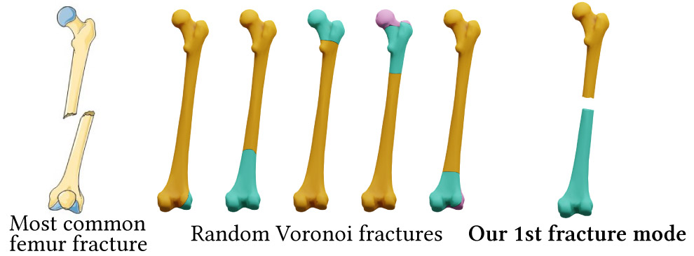
Figure 15. A healthy femur will usually break at the mid-shaft (see e.g., [Adnan et al., 2012]), as our first fracture mode correctly identifies, unlike Voronoi-based algorithms. Left image by Servier Medical Art under CC BY-SA 3.0.

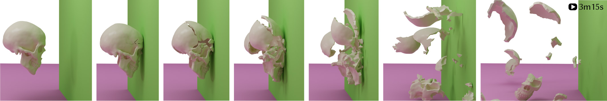
Figure 16. Ouch, my head hurts!

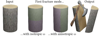
Figure 17. We can simulate the natural breaking tendencies of anisotropic materials like wood through weights in our vector valued discontinuity.

5. Experiments & Comparisons

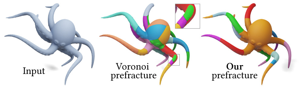
Figure 22. The pieces generated by Voronoi-based methods can be extremely unrealistic (center). By combining all the possible fractures in all our modes into a single prefractured mesh, we can provide a zero-extra-realtime-cost alternative to procedural algorithms.

Our proposed fracture modes naturally identify the regions of a shape that are geometrically weak, as opposed to existing procedural prefracture algorithms. We make this explicitly clear in Figs. 3 and 15, where existing prefracture work fails to identify even the most obvious intuitive breaking patterns which are present in our first (non-trivial) fracture mode. Even in less didactic examples, Voronoi-based prefracture methods result in convex, unrealistic and easily recognizable pieces (see Figs. 22 and 2), while our fracture modes are realistic and can produce a much wider set of shapes.

“Realism” in a fracture simulation is a hard quantity to evaluate; however, there exist works on structural analysis like [Zhou et al., 2013] that idenfity the weakest regions of a given object. In Fig. 6, we show how our fracture modes produce breaking patterns that align both with their analysis as well as with their real-life experiments.

We model heterogeneous and anisotropic materials by incorporating a vector field $\eta:\Omega\rightarrow\mathbb{R}^{d}$ to the discontinuity energy:

(26) $$E_{D}(u)=\sum_{i=1}^{p}\sqrt{\int_{S_{i}}\|\eta(x)\circ D(u,x)\|^{2}dx}\,,$$

where $\circ$ denotes Hadamard (elementwise) multiplication. In Fig. 18, we experiment with varying the magnitude of $\eta$ as an artist control tool to designate regions that should not fracture. In Fig. 17, we make $\eta=(10,10,1)$ to favour vertical faults over horizontal ones.

5.1. Fracture simulations

Our proposed method is ideal for its use in interactive applications. In Fig. 4, we show screenshots of our 2D realtime fracture interactive app. The user can cause different impacts on the object and see the fracture patterns that result from them by projecting onto our fracture modes.

The interactive Computer Graphics application par excellence is video games. In Fig. 7, we show a prototype where our precomputed fracture modes for a Space Wizard Vehicle can be stored so that the player sees different fracture behaviours depending on the received impact. In Fig. 14, we precompute the fracture modes for two different vehicles and show how they break under a similar impact.

Our algorithm can be used for any realtime fracture application, from simple objects breaking into solid pieces in the foreground of an animation (see Fig. 13) to thin shells shattering upon impact (see Figs. 19 and 18). In Fig. 16, we use our fracture modes to simulate a human skull breaking into many pieces upon impact with a wall.

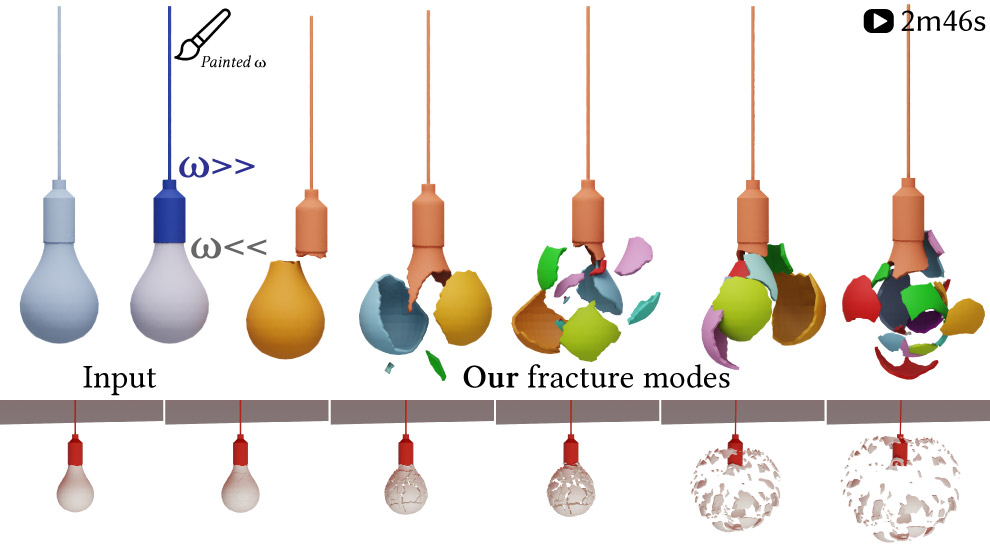
Figure 18. The magnitude of our $\eta$ parameter can be painted into our input to signal areas that shouldn’t fracture; e.g., in objects with different materials.

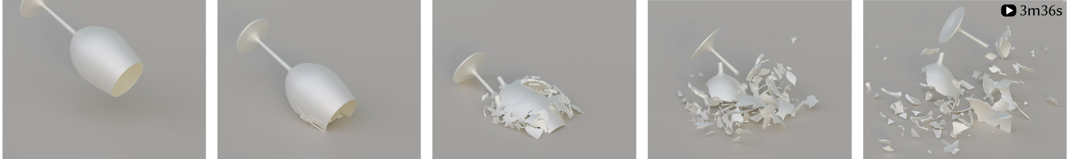
Figure 19. A glass cup shatters, resulting in many non-convex pieces that would be impossible to obtain with Voronoi-based prefracture methods.

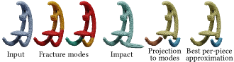
Figure 20. Our modes’ global nature (left) means some regions can be artificially linked (right middle). We could solve this by exchanging our mode projection for the least-squares best constant-per-piece approximation (right)

6. Limitations & Future Work

Our fracture modes method is intended for stiff brittle fracture. We conjecture that general rigid fracture and even ductile fracture simulation could also benefit from our sparse-norm formulation. In future work, we would like to improve the performance of our precomputation optimization. We experimented with Manopt [Boumal et al., 2014], but so far observed significantly slower performance than our proposed method. For very large meshes, the projection step could exceed CPU usage allowances for realtime applications. It may be possible to conduct this entirely on the GPU.

Our fracture modes are global in nature, meaning they create relations between regions of the object that will not typically fracture together (unlike other prefracture methods like [Oh et al., 2012]). A way of preventing a fracture in one location from also causing an undesired fracture elsewhere is to use our modes only to identify the pieces that could break off of an object in the precomputation step, and swap our realtime impact projection for a least squares constant-per-piece approximation (see Fig. 20).

Our use of an exploded mesh $\tilde{\Omega}$ allows us to expand the usual finite element hat function basis to include discontinuities along element boundaries. This mesh dependency is not present in traditional Voronoi or plane-cutting prefracture algorithms, and can lead to visible artifacts if the simulation mesh is too coarse. We alleviate it with post-facto smoothing (Section 3.6). Another way of reducing it (at a performance cost) would have been to include basis functions with sub-mesh-resolution discontinuities in the style of XFEM [Kaufmann et al., 2009; Chitalu et al., 2020].

Our algorithm is designed to fit into realtime rigid body simulations like those encountered in video games. Thus, our outputs will not contain partial fractures (unlike e.g., [Müller et al., 2013]).

Secondary fractures were not included in our simulations. Computing a new set of fracture modes for each piece would exceed realtime constraints. While one could obtain plausible secondary fractures by restricting our precomputed fracture modes and pattern to each primary fracture piece (see inset), there is no guarantee that these would match the individual piece’s fracture modes.

Our fracture mode computation considers only the magnitude of the vector-valued discontinuity and disregards its direction. Promising future work could include treating tangential and normal components differently as a way of simulating different material properties.

Our method belongs to the class of prefracture, not dynamic algorithms. Nonetheless, our method can be evaluated on dynamic fracture benchmarks like the notched block in [O’Brien and Hodgins, 1999]: if a given fracture plane is contained in one of our fracture modes, it can be present in the fractured output (see Fig. 21). The fracture fault will be the same regardless of the directionality of the impact. This deviates from the real-world mechanical behaviour, where faults will be different for brittle materials under uniaxial tension, pure shear, and torsion loads (see [Lawn, 1993], Chap. 2).

We hope our introduction of fracture eigenmodes inspires the realtime simulation community further to use the well-studied tools of modal analysis to this rich problem, and the broader Computer Graphics research community to look at other open problems with this modal lens.

Figure 21. If a given fracture mode is contained in our fracture modes, it can occur under any directional impact, as shown in this simple example inspired by O’Brien and Hodgins [1999].

Appendix A Canonical conic program form of Eq. (16)

Let us define a sparse matrix $\mathbf{D}\in\mathbb{R}^{pd×d(d+1)m}$ that operates on a deformation map and evaluates the vector-valued discontinuities at all the relevant integration quadrature points. The ordering of the rows of $\mathbf{D}$ is arbitrary, and we choose it such that $\mathbf{D}$ can be separated into $d$ blocks, one for each quadrature point.

For example, in the case $d=2$, we choose said ordering such that the first $p$ rows of $\mathbf{D}\mathbf{u}$ are the vector-valued edge-wise discontinuity

$$\sqrt{\frac{l_{e}}{2}}\mathbf{d}\left(\frac{1}{\sqrt{3}}\right)$$

from Eq. (13) and the last $p$ rows of $\mathbf{D}\mathbf{u}$ correspond to

$$\sqrt{\frac{l_{e}}{2}}\mathbf{d}\left(\frac{-1}{\sqrt{3}}\right)\,.$$

Since $\mathbf{Q}$ is positive semi-definite, we can write it as $\mathbf{Q}=\mathbf{R}^{\top}\mathbf{R}$ for some matrix $\mathbf{R}$. Define

(27) $$\mathbf{Y}_{e}=(\mathbf{D}\mathbf{u})_{e}\,,\forall e=1,\dots,2p,$$

where $l_{e}$ is the length of edge $e$. Next, define

(28) $$\qquad\mathbf{r}_{i}=(\mathbf{R}\mathbf{u})_{i}\,,\forall i=1,\dots,d(d+1)m.\quad$$

Then, Eq. (16) can be written in the canonical form

(29) $$\mathop{\text{argmin}}_{\mathbf{u},t,\mathbf{Y},\mathbf{z}}\begin{bmatrix}1\\ \mathbf{0}\\ \mathbf{0}\\ \mathbf{0}\\ \displaystyle\mathbf{1}\\ \end{bmatrix}^{\top}\begin{bmatrix}t\\ \mathbf{r}\\ \mathbf{u}\\ \mathbf{Y}\\ \mathbf{z}\\ \end{bmatrix}$$

subject to

$$t\geq\sqrt{\mathbf{r}_{1}^{2}+\ldots+\mathbf{r}_{d(d+1)m}^{2}}$$

$$\mathbf{z}_{e}\geq\sqrt{\sum_{s=0}^{d-1}\left\|\mathbf{Y}_{e+sp}\right\|_{2}^{2}}\;\;\forall e=1,\dots,p$$

$$\mathbf{Y}=\mathbf{D}\mathbf{u}$$

$$\mathbf{r}=\mathbf{R}\mathbf{u}$$

$$\mathbf{c}^{\top}\tilde{M}\mathbf{u}=1$$

$$\mathbf{U}^{j}\tilde{M}\mathbf{u}=0\,,\quad\forall j=1,\dots,i-1.$$

Appendix B Efficient conic program from Section 3.7

Let $\mathbf{C}$ be the $\mathbb{R}^{(d+1)m\times m}$ matrix of ones and zeros that transfers values from elements to vertices in the exploded mesh, and let us assume now that we are storing per-element deformations in vectors $\mathbf{v},\mathbf{U}_{j},\mathbf{c}\in\mathbb{R}^{dm}$. Then, our conic problem from Appendix A becomes

(30) $$\mathop{\text{argmin}}_{\mathbf{v},t,\mathbf{Y},\mathbf{z}}\begin{bmatrix}1\\ \mathbf{0}\\ \mathbf{0}\\ \mathbf{0}\\ \displaystyle\mathbf{1}\\ \end{bmatrix}^{\top}\begin{bmatrix}t\\ \mathbf{r}\\ \mathbf{v}\\ \mathbf{Y}\\ \mathbf{z}\\ \end{bmatrix}$$

subject to

$$t\geq\sqrt{\mathbf{r}_{1}^{2}+\ldots+\mathbf{r}_{d(d+1)m}^{2}}$$

$$\mathbf{z}_{e}\geq\sqrt{\sum_{s=0}^{d-1}\left\|\mathbf{Y}_{e+sp}\right\|_{2}^{2}}\;\;\forall e=1,\dots,p$$

$$\mathbf{Y}=\mathbf{D}\mathbf{C}\mathbf{v}$$

$$\mathbf{r}=\mathbf{R}\mathbf{C}\mathbf{v}$$

$$\mathbf{c}^{\top}\tilde{M}\mathbf{u}=1$$

$$\mathbf{U}^{j}\tilde{M}\mathbf{u}=0\,,\quad\forall j=1,\dots,i-1.$$

By construction, $\mathbf{Q}\mathbf{C}\mathbf{v}=0\Rightarrow\mathbf{R}\mathbf{C}\mathbf{v}=0$, which means we can remove $t$ and $\mathbf{r}$ as variables entirely. Further, since the vector-valued discontinuity is constant across element boundaries, $\mathbf{Y}_{e}=\mathbf{Y}_{e+sp}$, with $s=0,\dots,d-1$, meaning that we can remove the summation from the $z_{e}$ cone and consider only the first $p$ rows of $\mathbf{Y}$. This leads to the equivalent, simpler conic program

(31) $$\mathop{\text{argmin}}_{\mathbf{v},\mathbf{Y}}\begin{bmatrix}\mathbf{0}\\ \mathbf{0}\\ \displaystyle\mathbf{1}\\ \end{bmatrix}^{\top}\begin{bmatrix}\mathbf{v}\\ \mathbf{Y}\\ \mathbf{z}\\ \end{bmatrix}$$

subject to

$$\mathbf{z}_{e}\geq\sqrt{d\left\|\mathbf{Y}_{e}\right\|_{2}^{2}}\;\;\forall e=1,\dots,p$$

$$(\mathbf{Y})_{e}=(\mathbf{D}\mathbf{C}\mathbf{v})_{e}\;\;\forall e=1,\dots,p$$

$$\mathbf{c}^{\top}\mathbf{C}^{\top}\mathbf{M}\mathbf{C}\mathbf{v}=1$$

$$\mathbf{U}^{j}\mathbf{C}^{\top}\mathbf{M}\mathbf{C}\mathbf{v}=0\,,\quad\forall j=1,\dots,i-1.$$