Leveraging blur information for plenoptic camera calibration

Abstract

This paper presents a novel calibration algorithm for plenoptic cameras, especially the multi-focus configuration, where several types of micro-lenses are used, using raw images only. Current calibration methods rely on simplified projection models, use features from reconstructed images, or require separated calibrations for each type of micro-lens. In the multi-focus configuration, the same part of a scene will demonstrate different amounts of blur according to the micro-lens focal length. Usually, only micro-images with the smallest amount of blur are used. In order to exploit all available data, we propose to explicitly model the defocus blur in a new camera model with the help of our newly introduced Blur Aware Plenoptic (BAP) feature. First, it is used in a pre-calibration step that retrieves initial camera parameters, and second, to express a new cost function to be minimized in our single optimization process. Third, it is exploited to calibrate the relative blur between micro-images. It links the geometric blur, i.e., the blur circle, to the physical blur, i.e., the point spread function. Finally, we use the resulting blur profile to characterize the camera’s depth of field. Quantitative evaluations in controlled environment on real-world data demonstrate the effectiveness of our calibrations.

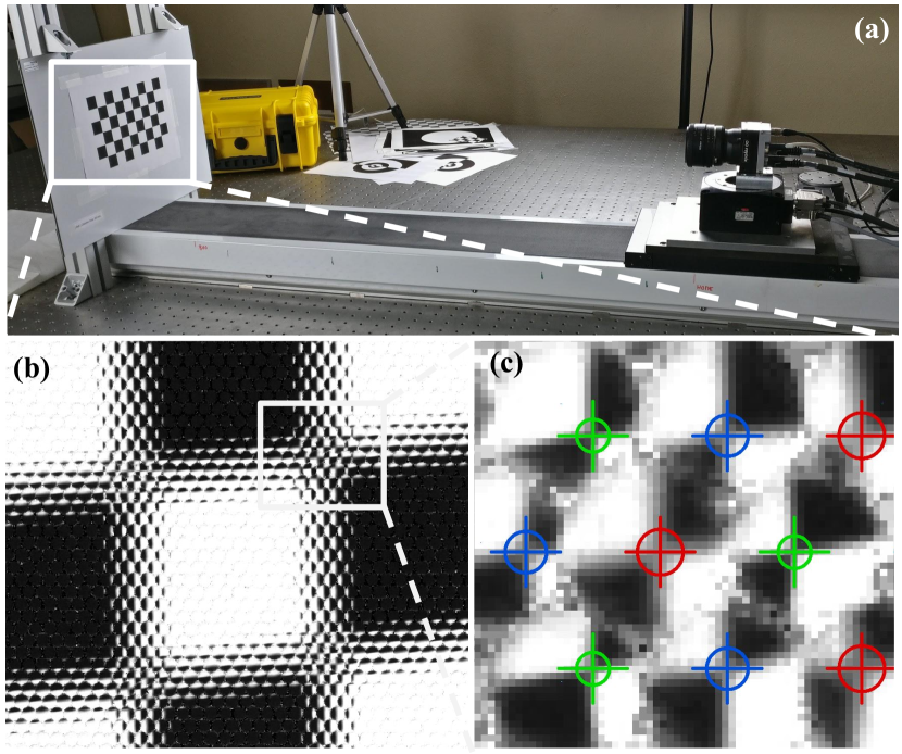
Figure 1: The Raytrix R12 multi-focus plenoptic camera used in our experimental setup (a), along with a raw image of a checkerboard calibration target (b). The image is composed of several micro-images with different amounts of blur, arranged in a hexagonal grid. In each micro-image, our Blur Aware Plenoptic (BAP) feature is illustrated by its center and its blur circle (c).

1 Introduction

From Lumigraph Lippmann1911b (23) to commercial plenoptic cameras Ng2005b (28, 35), several designs have been proposed to capture information that cannot be captured by conventional cameras. Said cameras capture only one point of view of a scene, whereas a plenoptic camera is a device that allows to retrieve spatial as well as angular information. A same point from a scene is projected into multiple observations on the sensor. For instance, this redundant information can be used for digitally refocusing and rendering Bishop2012 (1) or for depth estimation Johannsen2017b (18).

This paper focuses on plenoptic cameras based on a micro-lenses array (MLA) placed between a main lens and a sensor as illustrated in Figure 3. The specific design of such a camera allows to multiplex both types of information onto the sensor in the form of a micro-images array (MIA), as shown in Figure 1, but implies a trade-off between the angular and spatial resolutions Georgiev2006 (10, 21, 12). It is balanced according to the MLA position with respect to the main lens focal plane and the sensor plane, corresponding to unfocused Ng2005b (28) or focused Perwass2010c (35, 13) configurations.

To further extend the depth of field (DoF) of the plenoptic camera, a multi-focus configuration has been proposed by Perwass2010c (35, 13). In this setup, the MLA is composed of several micro-lenses with different focal lengths. The same part of a scene will be more or less focused according to the micro-lens’ type. Usually, only micro-images with the smallest amount of blur are used. Alternatively, specific patterns are used to exploit the information Palmieri2017 (33). If one were able to relate the camera parameters to the amount of blur in the image, all information could be used simultaneously, without distinction between types of micro-lenses. As a first step in that direction, we propose a calibration method that takes advantage of blur information.

Calibration is an initial step for applications using plenoptic imaging. Conventional cameras are usually modeled as pinhole or thin lens. Due to the complexity of plenoptic cameras’ design, the developed models are generally high dimensional. Specific calibration methods have to be proposed to retrieve the intrinsic parameters of these models.

1.1 Related work

Unfocused plenoptic camera calibration.

In the unfocused configuration, the main lens is focused at the MLA plane and the sensor plane is placed at the MLA focal plane. The MLA is therefore focused at infinity, thus calling this configuration unfocused. The calibration of such plenoptic cameras Ng2005b (28) has been widely studied in the literature. Most approaches rely on a thin-lens model for the main lens and an array of pinholes for the micro-lenses. Dansereau2013c (7) introduced a model to decode the pixels into rays, drawing inspiration from Grossberg2005 (14), for the Lytro plenoptic camera Ng2005b (28). Their model is not directly associated with physical parameters and is based on corner detection in reconstructed sub-aperture images. Zhou2019 (51) proposed a practical two-step calibration method for unfocused plenoptic cameras. Their model describes the camera physical parameters but still requires feature points extracted in reconstructed SAIs. Bok2014 (2) formulated a geometric projection model to estimate intrinsic and extrinsic parameters by utilizing raw images directly to avoid errors from reconstruction steps. Their method includes analytical solution and non-linear optimization of the reprojection error of a novel line feature to overcome the difficulties in finding checkerboard corners. Shi2016 (36) proposed a detailed model of a plenoptic camera in the context of particle image velocimetry (PIV). Based on linear optics, they derived a model based on ray-tracing: contrarily to previous methods, they modeled the main lens and each micro-lens as thin-lenses. Hahne2018b (15) developed a ray model by ray-tracing from the sensor side to the object space. They consider only the chief ray, connecting micro-image centers to the exit pupil center. OBrien2018 (32) introduced a projection model used for their calibration method suited both for unfocused and focused plenoptic cameras. They present a new feature called plenoptic disc, similar in nature to the circle of confusion (CoC) and defined by its center and its radius. Their feature parametrization is in 3D and is in one-to-one correspondence with point positions in the camera frame, as it is detected in reconstructed image. Zhao2020 (50) recently presented a metric calibration method for unfocused plenoptic camera only also based on the plenoptic disc but directly from raw image.

In summary, most of the above methods require reconstructed images (SAIs) to extract features, and limit their model to the unfocused configuration, i.e., setting the sensor plane at the micro-lens focal plane. Therefore those models cannot be directly extended to the focused or multi-focus plenoptic camera.

Focused plenoptic camera calibration.

With the arrival of commercial focused plenoptic cameras Lumsdaine2009b (24, 35), new calibration methods have been proposed. In this configuration, the micro-lenses focus on an intermediate image plane. Johannsen2013b (17) formulated a general reprojection model in terms of the physical parameters of a Raytrix camera Perwass2010c (35). They proposed a metric calibration and distortions correction using a grid of circular patterns. This work considered a relatively simple model of lens distortion and required careful initialization of the optimization to converge due to high sensibility to local minima. Heinze2016b (16) improved the previous model by considering more sophisticated models of the main lens distortions. They introduced new parameters including the tilt and shift for the main lens. They are able to distinguish each micro-lens type, calibrating then the distance between the MLA and the sensor for each one but in separated calibration processes. The projection model and the metric calibration procedure are incorporated in the RxLive software of Raytrix GmbH. Strobl2016 (37) presented a step-wise calibration approach to overcome the fragility of the initialization which hinders the final optimization. They first determined main lens parameters, then estimated MLA parameters. However, their calibration framework relied on reconstructed total focus images. Zeller2014 (44) introduced two new methods to calibrate a focused plenoptic camera and depth images obtained from it. In further works Zeller2016a (45, 46), they improved the camera projection model by modeling the main lens as a thin lens instead of a pinhole. The calibration process uses the reconstructed total focus image and virtual depth map to compute 3D observations.

All previous methods rely on reconstructed images (SAIs), which can lead to the introduction of errors in the reconstruction step as well as in the calibration process. Usually, computation of reconstructed images requires camera parameters and/or depth information to avoid artifacts and reconstruction error. To overcome this chicken and egg problem, several calibration methods focus on using only raw plenoptic images. Zhang2016a (48) proposed a calibration method based directly on observations from raw images. They used a parallel bi-planar checkerboard to have a depth-scale prior. They considered a detailed model of the MLA geometry that accounts for non-planarity of the array. Zhang2018a (49) presented a multi-projection-center model based on the two planes parametrization Levoy1996 (22). They derived a calibration algorithm based on this model and projective transformation, suitable for both unfocused and focused plenoptic cameras. Noury2017b (30) presented a more complete geometrical model than the previous works. This model relates 3D points to their corresponding image projections, working directly with raw images. They developed a new detector to find checkerboard corners with sub-pixel accuracy in each micro-image. They introduced a new cost function based on reprojection errors of both checkerboard corners and micro-lens centers in raw image space. This enforces projected micro-lens centers to get closer to their corresponding MICs, and makes their method robust to wrong parameters initialization especially concerning those of the MLA. However, their method does not consider different types of micro-lenses and forces them to act as pinholes.

Several methods can account for the multi-focus setting. Bok2017 (3) extended their previous model Bok2014 (2) to work with the focused plenoptic camera. They did not explicitly model the micro-lens focal lengths but introduced two additional intrinsic parameters that account for the MLA setting. Each setting – one for each type of micro-lenses –, models a different distance between the MLA and the sensor. Their method can retrieve different intrinsics by running the optimization for each type separately. Nousias2017 (31) considered the geometric calibration of multi-focus plenoptic cameras. Their method allows to identify the micro-lens types and their spatial arrangement. It operates on checkerboard corners retrieved by a custom micro-image corner detector. Then, they applied their method on each type of micro-lens independently to retrieve specific intrinsic and extrinsic parameters for each configuration. Latter researches Bok2017 (3, 31, 30) have achieved improved performance through automation and accurate identification of feature correspondences in raw images. More recently, Wang2018 (43) proposed a geometric calibration method for focused plenoptic cameras based on virtual image points, establishing the mapping from object points behind the main lens and the MLA to image points on the sensor. Their method can be extended to calibrate multi-focus cameras by considering each type of micro-lenses individually.

In conclusion, most of these methods rely on simplified models for optic elements: the MLA misalignment is not considered, and the micro-lenses are modeled as pinholes thus not modeling their apertures. Some do not consider distortions of the main lens or restrict themselves to the focused case. Finally, few have considered the multi-focus case Heinze2016b (16, 3, 31, 43) but dealt with it in separate processes, leading to intrinsic and extrinsic parameters that vary depending on the type of micro-lens.

1.2 Contributions

We present a new calibration method for plenoptic cameras. To the best of our knowledge, it is the first to allow to calibrate the multi-focus plenoptic camera within a single process taking into account all types of micro-lenses simultaneously. To exploit all available information, we propose to explicitly include the defocus blur in a new camera model. Thus, we introduce a new Blur Aware Plenoptic (BAP) feature defined in raw image space that enables us to handle the multi-focus case. We present a new pre-calibration step using BAP features from white images to provide a robust initial estimation of camera parameters. We use our BAP features in a single optimization process that retrieves intrinsic and extrinsic parameters of a multi-focus plenoptic camera directly from raw plenoptic images of a checkerboard target.

Figure 2: Overview of our proposed method: first, the pre-calibration step retrieves initial camera parameters from white raw images at different apertures; then followed by the detection of BAP features that are used by the camera calibration process and calibration ot the relative blur; finally, once the camera is calibrated, it can be used, as addressed here, for profiling the camera, i.e., to characterize the working range of the camera. Other applications can be considered, such as metric depth estimation.

This paper extends our previous work Labussiere2020blur (20). In addition to our former contributions, we present here an ablation study of the camera parameters and add further comparisons with state-of-the-art calibration methods. A new camera setup has also been tested to validate the generalization of our method, and a simulation setup is proposed to evaluate our method on Lytro-like configuration. Moreover, we take advantage of our BAP features to develop a new relative blur calibration process to link the geometric blur to the physical blur, i.e., the circle of confusion (CoC) to the point-spread function (PSF). This enables us to fully take advantage of blur in image space. Finally, we propose to use the blur to profile the plenoptic camera in terms of depth of field (DoF).

1.3 Paper organization

An overview of our method is given in Figure 2. The remainder of this paper is organized as follows. First, we present the camera model and how we model blur with our BAP feature in section 2. Second, we explain in section 3 how we leverage raw white images in the proposed pre-calibration step to initialize camera parameters. Then, we detail the feature detection in section 4 and the calibration processes in section 5, i.e., the camera calibration and the relative blur calibration. Our experimental setup is presented in section 6. Finally, our results are given and discussed in section 7. The notations used in this paper are shown in Figure 3. Pixel counterparts of metric values are denoted in lower-case Greek letters. Bold font denotes vectors and matrices.

2 Camera and blur models

Figure 3: Focused plenoptic camera model in Galilean configuration with the notations used in this paper. Object points are projected by the main lens behind the MLA into a virtual intermediate space, and then re-imaged by each micro-lens onto the sensor.

2.1 The (multi-focus) plenoptic camera

We consider the focused plenoptic camera, especially the multi-focus case as described by Georgiev2012 (13, 35). The camera is composed of a main lens and photosensitive sensor with a micro-lenses array (MLA) in between, as illustrated in Figure 3. The multi-focus configuration implies that the micro-lenses array consists of $I$ different types of lenses. The setup corresponds to the multi-focus system described by Perwass2010c (35) with $I=3$. Note that our model can be applied to the single-focus plenoptic camera as well, corresponding then to the case where $I=1$. Finally, the unfocused configuration is a special case of our model where the micro-lens focal length is equal to the distance between the MLA and the sensor, i.e., $f=d$.

2.1.1 Main Lens

The main lens is modeled as a thin-lens and maps an object point to a virtual point in an intermediate space called the virtual space. An object at distance $a$ is then projected at a distance $b$ given the focal length $F$ according to the thin-lens equation

$$\frac{1}{F}=\frac{1}{a}+\frac{1}{b}\text{.}$$ ((1))

The main lens principal point is expressed as $\begin{bmatrix}u_{0}&v_{0}\end{bmatrix}^{\top}$ in image space. We model the main lens as parallel to the sensor plane. Deviations from this hypothesis will be compensated for by tangential distortion parameters. Furthermore, we define our camera reference frame as the main lens frame, with $\bm{O}$ being the origin, the $z$-axis coinciding with the optical axis and pointing outside the camera, and the $y$-axis pointing downwards. Distances are signed according to the following convention: $F$ is positive when the lens is convergent; distances are positive when the point is real, and negative when virtual.

2.1.2 Distortions

We consider distortions of the main lens. Distortions represent deviations from the theoretical thin lens projection model. To correct those errors, we model the radial and tangential components of the lateral distortions using the model of Brown-Conrady Brown1966 (4, 6). Depth distortions have also been studied by Heinze2016b (16, 45), but Zeller2017 (47, 29) both empirically observed that the effects of depth distortions, for large focal length and for large object distance, can be neglected compared to stochastic noise of the depth estimation process. Therefore, we do not include depth distortion in our model. A distorted point $\bm{p}=\begin{bmatrix}x&y&z&1\end{bmatrix}^{\top}$ expressed in the main lens frame after projection (i.e., in the virtual intermediate space) is thus transformed into $\bm{p}_{u}=\mathrm{\varphi}\!\left(\bm{p}\right)=\begin{bmatrix}x_{u}&y_{u}&z&1\end{bmatrix}^{\top}$ and is computed as

$$\left\{\begin{aligned} x_{u}=&~{}x\left(1+Q_{1}\varsigma^{2}+Q_{2}\varsigma^{4}+Q_{3}\varsigma^{6}\right)&\text{[radial]}\\ &+P_{1}\left(\varsigma^{2}+2x{}^{2}\right)+2P_{2}xy&\text{[tangential]}\\ y_{u}=&~{}y\left(1+Q_{1}\varsigma^{2}+Q_{2}\varsigma^{4}+Q_{3}\varsigma^{6}\right)&\text{[radial]}\\ &+P_{2}\left(\varsigma^{2}+2y{}^{2}\right)+2P_{1}xy&\text{[tangential]}\\ \end{aligned}\right.$$ ((2))

where $\varsigma^{2}={x^{2}+y^{2}}$. The three coefficients for the radial component are given by $\left\{Q_{1},Q_{2},Q_{3}\right\}$, and the two coefficients for the tangential by $\left\{P_{1},P_{2}\right\}$.

2.1.3 Micro-lenses array

We also model the micro-lenses as thin-lenses allowing to take into account blur in the micro-image. The MLA consists then of $I$ different lens types with focal lengths $f{}^{\left(i\right)}$ where $i\in[1\mathrel{{.}\,{.}}\nobreak I]$ which are focused on $I$ different planes. We make the hypothesis that all micro-lenses lie on the same plane. The MLA is approximately centered around the optic axis. We define the farthest micro-lens along the $(-x)$-axis and the $(-y)$-axis as the origin of the MLA frame, i.e., the center of the upper-left micro-lens. The coordinates axes are orientated the same way as the ones of the main lens. The structural organization of the lenses can be an orthogonal or hexagonal arrangement. The MLA origin is at a distance $D$ from the main lens and at a distance $d$ from the sensor.

Furthermore, a detected micro-image center (MIC) usually does not coincide with the optical center of the considered micro-lens. We take into account this deviation in opposition to orthographic projection of MICs which causes inaccuracy in decoded light field. Therefore, the principal point $\bm{c}{}^{k,l}_{0}$ of the micro-lens indexed by $\left(k,l\right)$ is given by

$$\bm{c}{}^{k,l}_{0}=\begin{bmatrix}u_{0}^{k,l}\\ v_{0}^{k,l}\end{bmatrix}=\frac{d}{D+d}\left(\begin{bmatrix}u_{0}\\ v_{0}\end{bmatrix}-\bm{c}_{k,l}\right)+\bm{c}_{k,l}\text{, }$$ ((3))

where $\bm{c}_{k,l}$ is the center of the micro-image $\left(k,l\right)$ expressed in pixel, as illustrated in Figure 3.

2.1.4 Micro-images array

Finally, each micro-lens produces a micro-image (MI) onto the sensor. The set of these micro-images has the same structural organization as the MLA. The data can therefore be interpreted as an array of micro-images, called by analogy the micro-images array (MIA). The MIA coordinates are expressed in image space. Let $\delta_{i}$ be the pixel distance between two arbitrary consecutive micro-images centers $\bm{c}_{k,l}$. With $s$ the metric size of a pixel, let $\Delta_{i}=s\delta_{i}$ be its metric value, and $\Delta_{\mu}$ be the metric distance between the two corresponding micro-lens centers $\bm{C}_{k,l}$. From similar triangles, the ratio $\lambda$ between them is given by

$$\lambda\triangleq\frac{D}{d+D}=\frac{\Delta_{\mu}}{\Delta_{i}}\Longleftrightarrow\Delta_{\mu}=\lambda\Delta_{i}=\frac{D}{d+D}\cdot\Delta_{i}\text{.}$$ ((4))

We make the hypothesis that $\Delta_{\mu}$ is equal to the micro-lens aperture.

2.1.5 Camera configuration

When the camera is in the unfocused configuration, the distance separating the sensor and the MLA is equal to the focal length of the micro-lenses, i.e., $d=f$. Dealing with the focused plenoptic camera, we usually consider two possible configurations as presented by Georgiev2009d (11): 1) Galilean, when objects are projected behind the image sensor; and 2) Keplerian, when objects are projected in front of the image sensor. When considering micro-lenses as thin-lenses, we have to take into account their focal lengths to configure the camera. In practice, considering an object projected at distance $b$ by the main lens, four cases are possible but only two are able to produce an exploitable image, i.e., with acceptable amount of blur, onto the sensor: $b<D$ and $f<d$ in Keplerian; and, $b>D$ and $f>d$ in Galilean. The condition $b>D$ can be achieved both when $F>D$ and $F<D$. The mode of operation is then constrained by the focal length of the micro-lenses, as suggested by Mignard-Debise2017 (27). We introduce then the definition of the internal configuration according to the micro-lens focal length as

$$\left\{\begin{aligned} &&f<d&\Longrightarrow&\text{Keplerian {internal} configuration}\text{, }\\ &&f>d&\Longrightarrow&\text{Galilean {internal} configuration}\text{.}\end{aligned}\right.$$ ((5))

2.2 Modeling blur within the plenoptic camera

From optics geometry, the image of a point from a circular lens not focused on the sensor can be modeled by the circle of confusion (CoC). Using a camera with a circular aperture, the blurred image is also circular in shape and is called the blur circle. From similar triangles and from the thin-lens equation (Eq. (1)), the signed blur radius of the image of a point at a distance $a$ from the lens is expressed as

$$\left\{\begin{aligned} &&r&=A\frac{d}{2}\left(\frac{1}{f}-\frac{1}{a}-\frac{1}{d}\right)&\text{[metric]}\\ &&\rho&={r}/{s}&\text{[pixel]}\\ \end{aligned}\right.$$ ((6))

with $s$ being the size of a pixel, and $A$ the aperture of this lens. In continuous domain, the response of an imaging system to a not in-focus point, i.e., the blur, can be expressed by the point-spread function (PSF). Let ${I}\left(x,y\right)$ be the observed blurred image of an object at a constant distance. The image can be computed as the convolution of the PSF noted $\mathrm{h}\!\left(x,y\right)$, with the in-focus image, ${I}^{*}\!\left(x,y\right)$, such as

$${I}\left(x,y\right)=\mathrm{h}\text{\,\textasteriskcentered~{}}{I}^{*}\!\left(x,y\right)\text{, }$$ ((7))

where  *  denotes the convolution operator. If the lens aperture is circular and the level of blur low, the PSF $\mathrm{h}\!\left(x,y\right)$ can be efficiently modeled by a two-dimensional Gaussian given by

$$\mathrm{h}\!\left(x,y\right)=\frac{1}{2\pi\sigma^{2}}\exp\left(-\frac{x^{2}+y^{2}}{2\sigma^{2}}\right)\text{, }$$ ((8))

where the spread parameter $\sigma$ is proportional to the blur circle radius $\rho$. Therefore, we can write

$$\sigma\propto\rho\Leftrightarrow\sigma=\kappa\cdot\rho$$ ((9))

where $\kappa$ is a camera constant that should be determined by calibration Pentland1987 (34, 39). Note that the spatially-variant spread parameter $\sigma$ thus depends on the object distance $a$.

The blur radius $\rho$ appears at several levels within the camera projection: in the blur introduced by the thin-lens model of the micro-lenses and in the formation of the micro-images while taking a white image. Each micro-lens $\left(k,l\right)$ projects virtual points onto the sensor at a position $\left(u,v\right)$, with a blur radius $\rho$ depending on the distance to the point and the micro-lens type.

2.3 BAP features and projection model

To leverage this blur information, we introduce a new Blur Aware Plenoptic (BAP) feature characterized by its center and its radius, noted $\bm{p}=\begin{bmatrix}u&v&\rho&1\end{bmatrix}^{\top}$. The BAP feature are visualized in Figure 1. Therefore, our complete plenoptic camera model allows us to link a scene point $\bm{p}_{w}=\begin{bmatrix}x&y&z&1\end{bmatrix}^{\top}$ to our new BAP feature $\bm{p}$ in homogeneous coordinates through each micro-lens $\left(k,l\right)$ such as

$$\begin{bmatrix}u\\ v\\ \rho\\ 1\end{bmatrix}\propto\mathsf{P}\!\left(i,k,l\right)\cdot\bm{T}_{\mu}\!\left(k,l\right)\cdot\mathrm{\varphi}\!\left(\bm{K}\!\left(F\right)\cdot\bm{T}_{c}\cdot\bm{p}_{w}\right)\text{, }$$ ((10))

where $\mathsf{P}\!\left(i,k,l\right)$ is the blur aware plenoptic projection matrix through the micro-lens $\left(k,l\right)$ of type $i$, and computed as

$$\mathsf{P}\!\left(i,k,l\right)=\bm{P}\left(k,l\right)\cdot\bm{K}\!\left(f{}^{\left(i\right)}\right)$$ ((11))

$$= \begin{bmatrix}{d}/{s}&0&u_{0}^{k,l}&0\\ 0&{d}/{s}&v_{0}^{k,l}&0\\ 0&0&\frac{\Delta_{\mu}}{2s}&-\frac{\Delta_{\mu}}{2s}d\\ 0&0&-1&0\end{bmatrix}\begin{bmatrix}1&0&0&0\\ 0&1&0&0\\ 0&0&1&0\\ 0&0&-1/f{}^{\left(i\right)}&1\end{bmatrix}\text{.}$$

$\bm{P}\left(k,l\right)$ is a matrix that projects the 3D virtual point onto the sensor and taking into account the blur radius. $\bm{K}\!\left(f\right)$ is the thin-lens projection matrix for the given focal length. $\bm{T}_{c}$ is the pose of the main lens with respect to the world frame and $\bm{T}_{\mu}\!\left(k,l\right)$ is the pose of the micro-lens $\left(k,l\right)$ expressed in the camera frame. The function $\mathrm{\mathrm{\varphi}}\!\left(\cdot\right)$ models the lateral distortions.

Finally, the projection model from Eq. (10) consists of a set $\Xi$ of $\left(16+I\right)$ intrinsic parameters to be optimized, including: the main lens focal length $F$, expressed in $\bm{K}\!\left(F\right)$, and its five lateral distortion coefficients $Q_{1}$, $Q_{2}$, $Q_{3}$, $P_{1}$, and $P_{2}$, expressed in $\mathrm{\varphi}\!\left(\cdot\right)$; the sensor translations, encoded in $d$ and $\left(u_{0},v_{0}\right)$ through Eq. (3), from $\bm{P}\left(k,l\right)$; the MLA pose, including its three rotations $\left(\theta_{x},\theta_{y},\theta_{z}\right)$ and three translations $\left(t_{x},t_{y},D\right)$, and the micro-lens pitch $\Delta_{\mu}$, expressed in $\bm{T}_{\mu}\!\left(k,l\right)$; and, the $I$ micro-lens focal lengths $f{}^{\left(i\right)}$, in $\bm{K}\!(f{}^{\left(i\right)})$.

2.4 Profiling the depth of field of the plenoptic camera

From calibrated camera parameters, we can compute the depth of field (DoF) of each micro-lens type and the blur profile – the blur radii as function of the object distance –, in order to profile the plenoptic camera. The analysis can be done with respect to the MLA pose, and then extended to object space by back-projection. A point at a distance $a$ from MLA is projected back into object space at a distance $a^{\prime}$ according to the thin-lens equation through the main lens, such as

$$a^{\prime}=\frac{\left(D-a\right)\cdot F}{\left(D-a\right)-F}\text{.}$$ ((12))

Let $r_{0}$ be the minimal acceptable radius of the CoC. The smallest diffraction-limited spot resolved by a lens in wave optics, i.e., the radius of the first null of the Airy disc, is $r^{*}=1.22\cdot\nu\cdot N^{*}$, where $\nu$ is the considered light wavelength, and $N^{*}=d/A$ is the working $f$-number of the lens. The minimal acceptable radius is the maximum between this limit and half the size of a pixel, such as $r_{0}=\max\left(r^{*}\text{, }{s}/2\right)$. For a a micro-lens of type $(i)$, the focus plane distance is given by

$$a_{0}^{(i)}=\left(\frac{1}{f^{(i)}}-\frac{1}{d}\right)^{-1}=\frac{df^{(i)}}{d-f^{(i)}}\text{.}$$ ((13))

Let $A$ be the micro-lens aperture, we derive then the far $a_{+}$ and near $a_{-}$ focus planes distances:

$$\left\{\begin{aligned} a_{+}^{(i)}&=\frac{dA\cdot a_{0}^{(i)}}{Af{}^{\left(i\right)}-2r_{0}\left(a_{0}^{(i)}-f{}^{\left(i\right)}\right)}&&\text{~{}~{}~{}~{}[far]}\\ a_{-}^{(i)}&=\frac{dA\cdot a_{0}^{(i)}}{Af{}^{\left(i\right)}+2r_{0}\left(a_{0}^{(i)}-f{}^{\left(i\right)}\right)}&&\text{~{}~{}~{}~{}[near]}\text{.}\\ \end{aligned}\right.$$ ((14))

The DoF of a micro-lens of type $(i)$ is computed as the distance between the near and far focus planes, such as

$$\mathrm{D\!O\!F}^{(i)}=\left|{a_{+}^{(i)}}\right|-\left|{a_{-}^{(i)}}\right|=\frac{Af{}^{\left(i\right)}\cdot a_{0}^{(i)}\cdot 2r_{0}\left(a_{0}^{(i)}-f{}^{\left(i\right)}\right)}{\left(Af{}^{\left(i\right)}\right)^{2}-4r_{0}^{2}\left(a_{0}^{(i)}-f{}^{\left(i\right)}\right)^{2}}.$$ ((15))

Note that to fully exploit the combined extended DoFs without gaps, the micro-lenses DoFs should either just touch or slightly overlap Perwass2010c (35). Finally, under this consideration, the total DoF of the plenoptic camera in MLA space is computed using the micro-lenses DoFs as

$$\mathrm{D\!O\!F}=\max_{i}\left\{\left|a_{+}^{(i)}\right|\right\}-\min_{i}\left\{\left|a_{-}^{(i)}\right|\right\}\text{.}$$ ((16))

We can finally plot the blur profile of the camera, along with the focal planes and the total DoF as illustrated by the Figure 10.

3 Pre-calibration using raw white images

The goal of the pre-calibration step is to provide a strong initial estimate of the camera parameters. Inspired from depth from defocus theory Subbarao1994 (40), we leverage blur information to estimate our blur radius by varying the main lens aperture and using the different micro-lenses focal lengths, in combination with parameters from the image space. This is achieved by using raw white images acquired with a light diffuser mounted on the main objective, and taken at different apertures. We then show how the blur radii are linked to camera parameters, thus enabling their initialization.

3.1 Micro-images array calibration

First, the micro-images array (MIA) is calibrated using raw white images. We compute the micro-image centers $\left\{\bm{c}_{k,l}\right\}$ by the intensity centroid method with sub-pixel accuracy Thomason2014 (42, 30, 41). The distance between two micro-image centers $\delta_{i}$ is then computed as the optimized edge-length of a fitted 2D regular grid mesh. The optimization is conducted by non-linear minimization of the distances between the grid vertices and the corresponding detected MICs. The pixel translation offset in image coordinates, $(\tau_{x},\tau_{y})$, and the rotation around the $\left(-z\right)$-axis, $\vartheta_{z}$, are also determined during the optimization process.

3.2 Deriving the micro-image radius

In white images taken with a light diffuser and a controlled aperture, each type of micro-lens produces a micro-image (MI) with a specific size and intensity. This provides a mean to distinguish between them (Figure 5). The process of capturing a white image is equivalent for the micro-lenses to imaging a white uniform object of diameter $A$ at a distance $D$. The imaging process is schematized in Figure 4. Using optics geometry, the image of this object, i.e., the resulting MI, corresponds to the image of an imaginary point $V$ constructed as the vertex of the cone passing through the main lens and the considered micro-lens. Let $a$ be the signed distance of this point from the MLA plane, expressed from similar triangles and Eq. (4) as

$$a=-D\frac{\Delta_{\mu}}{A-\Delta_{\mu}}=-{D}\left(A\left(\frac{d+D}{D}\cdot\frac{1}{\Delta_{i}}\right)-1\right)^{-1}\text{, }$$ ((17))

with $A$ being the main lens aperture. Note the minus sign is added because the vertex is always formed behind the MLA plane, and thus considered as a virtual object for the micro-lenses. Geometrically, the MI formed is the blur circle of this imaginary point $V$. Therefore, injecting the latter expression in Eq. (6), the metric MI radius $R$ is given by

$$R =\frac{\Delta_{\mu}}{2}d\left(\frac{1}{f}-\frac{1}{a}-\frac{1}{d}\right)$$

$$=\left(\frac{\Delta_{i}\cdot D}{d+D}\right)\cdot\frac{d}{2}\cdot\left(\frac{1}{f}+\left(A\left(\frac{d+D}{D}\cdot\frac{1}{\Delta_{i}}\right)-1\right)\frac{1}{D}-\frac{1}{d}\right)$$

$$=A\cdot\frac{d}{2D}+\left(\frac{\Delta_{i}\cdot D}{d+D}\right)\cdot\frac{d}{2}\cdot\left(\frac{1}{f}-\frac{1}{D}-\frac{1}{d}\right)\text{.}$$ ((18))

From the above equation, the MI radius $R$ depends linearly on the aperture of the main lens. However, the main lens aperture cannot be measured directly whereas we have access to the $f$-number value. Recall that the $f$-number of an optical system is the ratio of the system’s focal length $F$ to the aperture, $A$, given by $N={F}/{A}$. Finally, we can express the MI radius for each micro-lens focal length type $i$ as

$$\mathrm{R_{i}}\!\left(N^{-1}\right)=m\cdot N^{-1}+q_{i}$$ ((19))

with

$$m=\frac{dF}{2D}\text{~{}~{}~{}and~{}~{}~{}}q_{i}=\frac{1}{f{}^{\left(i\right)}}\cdot\left(\frac{\Delta_{i}\cdot D}{d+D}\right)\cdot\frac{d}{2}-\frac{\Delta_{i}}{2}\text{.}$$ ((20))

We thus relate the MI radius to the plenoptic camera parameters. It is a function of fixed parameters ($d,D,F$), measured parameters ($\Delta_{i}=s\cdot\delta_{i}$) and variable parameters ($N$ and $f{}^{\left(i\right)}$ with $i\in[1\mathrel{{.}\,{.}}\nobreak I]$).

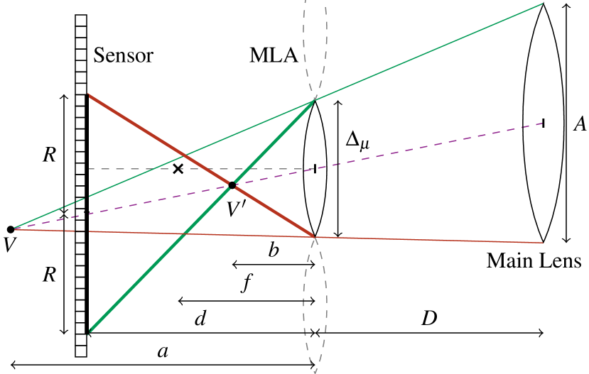
Figure 4: Formation of a micro-image with its radius $R$ through a micro-lens while taking a white image using a light diffuser, at an aperture $A$, in Keplerian internal configuration. The point $V$ is the vertex of the cone passing by the main lens and the considered micro-lens. $V^{\prime}$ is the image of $V$ by the micro-lens and $R$ is the radius of its blur circle.

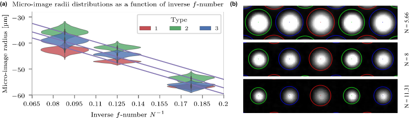
Figure 5: (a) Micro-image radii as function of the inverse $f$-number (in magenta), with their distributions represented by the violin-boxes, for our camera consisting of $I=3$ different types. (b) Each type of micro-lens is identified by its color (type $(1)$ in red, type $(2)$ in green, and type $(3)$ in blue) with its computed radius.

Let $\Omega$ be the set of parameters $\left\{m,q^{\prime}_{1},\dots,q^{\prime}_{I}\right\}$, where $q_{i}^{\prime}$ is the value obtained by

$$q_{i}^{\prime}=\frac{1}{f{}^{\left(i\right)}}\cdot\left(\frac{\Delta_{i}\cdot D}{d+D}\right)\cdot\frac{d}{2}=q_{i}+\frac{\Delta_{i}}{2}\text{.}$$ ((21))

They are used to compute the radius part of the BAP feature and to initialize the camera parameters.

Micro-image radii estimation.

From raw white images, we measure each MI radius $\mathsf{\varrho}=\left|R\right|/s$ in $\mathrm{p}\mathrm{i}\mathrm{x}\mathrm{e}\mathrm{l}$ based on image moments fitting. We use the second order central moments of the micro-image to construct a covariance matrix. The radius $\mathsf{\varrho}$ is proportional to the computed standard deviation $\sigma$. Recall that raw moments and centroid are given by

$$M_{{ij}}=\sum_{x,y}x^{i}y^{j}{I}\left(x,y\right) {\displaystyle\{{\bar{x}},\ {\bar{y}}\}=\left\{{\frac{M_{10}}{M_{00}}},{\frac{M_{01}}{M_{00}}}\right\}}\text{, }$$ and

and the central moments by

$$\mu_{{pq}}=\sum_{{x,y}}(x-{\bar{x}})^{p}(y-{\bar{y}})^{q}{I}\left(x,y\right)\text{.}$$ ((22))

The covariance matrix is then computed as

$$\mathrm{cov}\left[{I}\left(x,y\right)\right]=\frac{1}{\mu_{{00}}}\begin{bmatrix}\mu_{{20}}&\mu_{{11}}\\ \mu_{{11}}&\mu_{{02}}\end{bmatrix}=\begin{bmatrix}\sigma_{{xx}}&\sigma_{{xy}}\\ \sigma_{{yx}}&\sigma_{{yy}}\end{bmatrix}\text{.}$$ ((23))

We define $\sigma$ as the square root of the greatest eigenvalue of the covariance matrix, i.e.,

$$\sigma^{2}=\frac{\sigma_{{xx}}+\sigma_{{yy}}}{2}+\frac{\sqrt{{4\sigma_{{xy}}^{2}}+\left(\sigma_{{xx}}-\sigma_{{yy}}\right)^{2}}}{2}\text{.}$$ ((24))

The estimation is robust to noise, works under asymmetrical distribution and is easy to use, but requires a parameter $\alpha$ to convert the standard deviation $\sigma$ into a pixel radius $\mathsf{\varrho}=\alpha\cdot\sigma$. The parameter $\alpha$ is determined so that at least $98\%$ of the distribution is taken into account. According to the standard normal distribution $Z$-score table, $\alpha$ is picked up in $.Inourexperiments,weset$α= 2.357$asitbestfitsourmeasurements.\par Recallthatthepixel\acs{MI}radiusisgivenby$$\mathsf{\varrho}$= —R—/s$.Themetricradiusiseitherpositiveifformedaftertheraysinversion,asin\autoref{fig:blurradius},ornegativeifbefore,andthusdependsonthe\textit{internal}configurationsuchas\begin{equation}R=\left\{\begin{aligned} \mathsf{\varrho}\cdot s&&\text{[Keplerian {internal} configuration]}\text{, }\\ -\mathsf{\varrho}\cdot s&&\text{[Galilean {internal} configuration]}\text{.}\end{aligned}\right.\end{equation}\par\par$

Coefficients estimation.

Given several raw white images taken at different apertures, we estimate the parameters $\Omega$, i.e., the coefficients of Eq. (19), for each type of micro-image. Note that the standard full-stop $f$-number conventionally indicated on the lens differs from the real $f$-number. We use then the $f$-number calculated from the aperture value $\mathrm{A\!V}$ by $N=\sqrt{2^{\mathrm{A\!V}}}$. The coefficient $m$ is a function of fixed physical parameters independent of the micro-lens focal lengths and the main lens aperture. Therefore, we obtain a set of linear equations, sharing the same slope, but with different $y$-intercepts. With $\bm{X}=\begin{bmatrix}m&q_{1}&\dots&q_{I}\end{bmatrix}^{\top}$, the set of equations can be linearly rewritten as

$$\bm{A}\bm{X}=\bm{B}\text{, }\text{ and then }\bm{X}=\left(\bm{A}^{\top}\bm{A}\right)^{-1}\bm{A}^{\top}\bm{B}$$

where the matrix $\bm{A}$, containing the $f$-numbers and a selector of the corresponding $y$-intercept coefficient, and the vector $\bm{B}$, containing the radii measurements, are constructed by arranging the terms given the focal length at which they have been calculated. Finally, we compute $\bm{X}$ with a least-square estimation. Figure 5 shows an example of radii distributions from our experiments computed from white images taken at several $f$-numbers, and the estimated linear functions. In practice, at least two aperture configurations are required. More can be used to improve the estimation but at the condition that radii measurement distributions are distinguishable from each others, with small overlap.

3.3 Camera parameters initialization

First, the pixel size $s$ is set according to the manufacturer values. The main lens focal length $F$ is also initialized from them. Given the parameters $\Omega$ and the focus distance $h$, the parameters $d$ and $D$ are initialized as

$$d\longleftarrow\frac{2mH}{F+\xi\cdot 4m}\text{~{}~{}~{}~{}and~{}~{}~{}~{}}D\longleftarrow H-\xi\cdot 2d\text{, }$$ ((26))

with $\xi=1$ (resp., $\xi=-1$) in Galilean (resp., Keplerian) internal configuration, and where $H$ is given by Eq. (17) of Perwass2010c (35),

$$H=\left|\frac{h}{2}\left(1-\sqrt{1-4\frac{F}{h}}\right)\right|\text{.}$$ ((27))

For completeness, note that the unfocused configuration can be initialized with $d\leftarrow 2m$ and $D\leftarrow F$.

In a second step, all distortions coefficients are set to zero. The principal point is set as the center of the image. The sensor plane is thus set parallel to the main lens plane, with no rotation, at a distance $-\left(D+d\right)$. Seemingly, the MLA plane is initially set parallel to the main lens plane at a distance $-D$. From the pre-computed MIA parameters, the MLA translation takes into account the $(x,y)$-offsets $\left(-s\tau_{x},-s\tau_{y}\right)$ and the rotation around the $z$-axis is initialized with $-\vartheta_{z}$. The micro-lenses pitch $\Delta_{\mu}$ is set according to Eq. (4), where the ratio $\lambda$ is computed using Eq. (26) such as

$$\lambda\longleftarrow\frac{F}{F+2m}\text{.}$$ ((28))

Finally, the initial micro-lenses’ focal lengths are also computed from the parameters $\Omega$ as follows

$$f{}^{\left(i\right)}\longleftarrow\frac{d}{2\cdot q_{i}^{\prime}}\cdot\Delta_{\mu}\text{.}$$ ((29))

Experiments will show that the initial model is close to the optimized model.

4 BAP features detection in raw images

At this point, the MIA is calibrated and micro-images centers are extracted. The raw images are devignetted by dividing them by a white raw image taken with the same aperture. We based our method on a checkerboard calibration pattern. The detection process is divided into two steps: 1) checkerboard images are processed to extract corners at position $\left(u,v\right)$; and 2) with the set of parameters $\Omega$ and the associated virtual depth estimate for each corner, the corresponding BAP feature is computed in image space.

4.1 Computing blur radius through micro-lens

To respect the $f$-number matching principle Perwass2010c (35), we configure the main lens $f$-number such that the micro-images fully tile the sensor without overlap. In this configuration the working $f$-number of the main imaging system and the micro-lens imaging system should match. We consider the general case of measuring an object $\bm{p}$ at a distance $a$ from the main lens. First, $\bm{p}$ is projected through the main lens according to the thin lens equation, ${1}/{F}={1}/{a}+{1}/{b}$, resulting in a point $\bm{p}^{\prime}$ at a distance $b$ behind the main lens, i.e., at a distance $a^{\prime}=D-b$ from the MLA. From Eq. (6), the metric radius of the blur circle $r$ of a point $\bm{p}^{\prime}$ at distance $a^{\prime}$ through a micro-lens of type $(i)$ is expressed as

$$r =\left(\frac{\Delta_{i}D}{d+D}\right)\cdot\frac{d}{2}\cdot\left(\frac{1}{f{}^{\left(i\right)}}-\frac{1}{a^{\prime}}-\frac{1}{d}\right)$$

$$=\underbrace{\frac{\Delta_{i}\cdot D}{d+D}\cdot\frac{d}{2}\cdot\frac{1}{f{}^{\left(i\right)}}}_{=q^{\prime}_{i}\text{~{}[\autoref{eq:qprime}]}}-\underbrace{\frac{\Delta_{i}\cdot D}{d+D}\cdot\frac{d}{2}\cdot\frac{1}{d}}_{=\Delta_{\mu}/2\text{~{}[\autoref{eq:mlinterdist}]}}-\underbrace{\frac{\Delta_{i}\cdot D}{d+D}}_{=\Delta_{\mu}\text{~{}[\autoref{eq:mlinterdist}]}}\cdot\frac{d}{2}\cdot\frac{1}{a^{\prime}}$$

$$=\left(-\Delta_{\mu}\cdot\frac{d}{2}\right)\cdot\frac{1}{a^{\prime}}+\left(q_{i}^{\prime}-\frac{\Delta_{\mu}}{2}\right)\text{.}$$ ((30))

In practice, $a^{\prime}$ and $d$ cannot be measured in raw image space, but the virtual depth can, as it will be shown in the next subsection. Virtual depth refers to relative depth value obtained from disparity. It is defined as the ratio between the signed object distance $a^{\prime}$ and the sensor distance $d$:

$$\upsilon=-\frac{a^{\prime}}{d}\text{.}$$ ((31))

The sign convention is reversed for virtual depth computation. Distances are negative in front of the MLA plane. If we re-inject the virtual depth in subsection 4.1, taking caution of the sign, and using Eq. (4), we can derive the radius of the blur circle of a point $\bm{p}^{\prime}$ at a distance $a^{\prime}$ from the MLA by

$$r =\frac{\lambda\Delta_{i}}{2}\cdot\upsilon^{-1}+\left(q_{i}^{\prime}-\frac{\lambda\Delta_{i}}{2}\right)\text{.}$$ ((32))

This equation allows to express the pixel radius of the blur circle $\rho=r/s$ associated to each point having a virtual depth without explicitly evaluating the physical parameters $A,D,d,F\text{ and }f{}^{\left(i\right)}$ of the camera, directly in image space.

4.2 Features extraction

First, we detect corners in raw images using the detector introduced by Noury2017b (30) with sub-pixel accuracy in each micro-image. With a plenoptic camera, contrarily to a classic camera, a same point in object space is projected into multiple observations onto the sensor. The checkerboard is designed and positioned so that the sets of observations are sufficiently far from each others to be clustered. We use the DBSCAN algorithm Ester1996 (9) to identify the clusters. We then associate each point with its cluster of observations.

Secondly, once each cluster is identified, we compute the virtual depth $\upsilon$ from the disparity. Let $\Delta\!\bm{C}_{1-2}$ be the distance between the centers of the micro-lenses $\bm{C}_{1}$ and $\bm{C}_{2}$, i.e., the baseline. Let $\Delta\!\bm{p}=\left|\bm{p}_{1}-\bm{p}_{2}\right|$ be the Euclidean distance between images of the same point in corresponding micro-images. The virtual depth $\upsilon$ is calculated with the intercept theorem:

$$\upsilon=\frac{\Delta\!\bm{C}_{1-2}}{\Delta\!\bm{C}_{1-2}-\Delta\!\bm{p}}=\frac{\eta\cdot\Delta_{\mu}}{\eta\cdot\Delta_{\mu}-\Delta\!\bm{p}}=\frac{\eta\cdot\lambda\Delta_{i}}{\eta\cdot\lambda\Delta_{i}-\Delta\!\bm{p}}\text{.}$$ ((33))

If we consider two adjacent micro-lenses, the baseline $\Delta\!\bm{C}_{1-2}$ is just the diameter of a micro-lens, i.e., $\Delta_{\mu}=\lambda\Delta_{i}$ and $\eta=1$. For further apart micro-lenses the baseline is a multiple of that diameter, where $\eta$ is not necessarily an integer. To handle noise in corner detection, we use a median estimator to compute the virtual depth of the cluster, taking into account all combinations of point pairs in the disparity estimation.

Finally, we compute the BAP features from Eq. (32), using the set of parameters $\Omega$ and the available virtual depth $\upsilon$. In each frame $n$, for each micro-image $\left(k,l\right)$ of type $(i)$ containing a corner at position $\left(u,v\right)$ in the image, the feature $\bm{p}{}^{n}_{k,l}$ is given by

$$\bm{p}{}^{n}_{k,l}=\begin{bmatrix}u&v&\rho&1\end{bmatrix}^{\top},\text{ with }\rho=r/s\text{.}$$ ((34))

In the end, our observations are composed of a set of micro-images centers $\left\{\bm{c}_{k,l}\right\}$ and a set of BAP features $\left\{\bm{p}{}^{n}_{k,l}\right\}$ allowing us to introduce two reprojection error functions corresponding to each set of features as explains in the next section.

5 Camera and relative blur calibration

To retrieve the parameters of our camera model (Eq. (10)), we use a calibration process based on non-linear minimization of reprojection errors. The camera calibration process is divided into three phases: 1) the initial intrinsics are provided by the pre-calibration step; 2) the initial extrinsics are estimated from the raw checkerboard images; and 3) the parameters are refined with a non-linear optimization leveraging our new BAP features. In parallel, using our BAP features, the blur proportionality coefficient of Eq. (9) is calibrated, by minimizing the relative blur in a new reprojection error with a non-linear optimization.

5.1 Camera model initialization

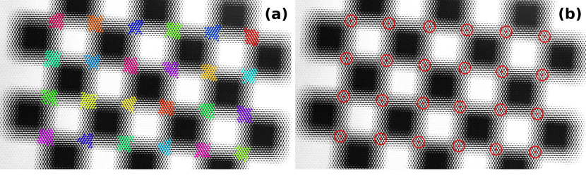
Figure 6: Checkerboard raw image with: (a) clusters of observations; (b) their barycenter used as approximation for extrinsics initialization.

Iterative optimization of non-linear cost functions are sensitive to initial parameters setting. To ensure convergence and to avoid falling into local minima during the process, the parameters must be carefully initialized close to the solution. Our pre-calibration step provides a strong initial solution for the optimization. Intrinsic parameters are initialized as explained in subsection 3.3 using only raw white images.

The camera poses $\left\{\bm{T}_{c}^{n}\right\}$, i.e., the extrinsic parameters, are initialized using the same method as by Noury2017b (30). For each cluster of observations, the barycenter is computed, as illustrated by Figure 6. Those barycenters can been seen as the projections of the checkerboard corners through the main lens using a standard pinhole model. For each frame, the pose is then estimated using the Perspective-n-Point (PnP) algorithm Kneip2011b (19), like in classic pinhole imaging system. To associate 3D-2D correspondences, we reproject checkerboard corners based on the estimated pose in image space and link them to their nearest cluster of observations.

5.2 Optimizing the camera parameters

By introducing blur in our model, we can optimize all parameters within one single optimization process. We propose a new cost function $\Theta$ taking into account the blur information of our new BAP feature. The cost is composed of two main terms both expressing errors in the image space: 1) the blur aware plenoptic reprojection error and 2) the main lens center reprojection error.

In the first term, for each frame $n$, each checkerboard corner $\bm{p}{}^{n}_{w}$ is reprojected into the image space through each micro-lens $\left(k,l\right)$ of type $(i)$ according to the projection model of Eq. (10) and compared to its observations $\bm{p}{}^{n}_{k,l}$. In the second term, the main lens center $\bm{O}$ is reprojected according to a pinhole model in the image space through each micro-lens $\left(k,l\right)$ and compared to its detected micro-image center $\bm{c}_{k,l}$. Let $\mathsf{S}=\left\{\Xi,\left\{\bm{T}_{c}^{n}\right\}\right\}$ be the set of intrinsic $\Xi$ and extrinsic $\left\{\bm{T}_{c}^{n}\right\}$ parameters to be optimized. The cost function $\Theta(\mathsf{S})$ is expressed as

$$\Theta({\mathsf{S}})=\sum\left\|\bm{p}{}^{n}_{k,l}-{\mathrm{\Pi}_{k,l}\left(\bm{p}{}^{n}_{w}\right)}\right\|^{2}+\sum\left\|\bm{c}_{k,l}-\mathrm{\Pi}_{k,l}\left(\bm{O}\right)\right\|^{2}\text{.}$$ ((35))

The optimization is conducted using the Levenberg-Marquardt algorithm.

5.3 Relative blur calibration using BAP features

Relative blur estimation has been studied by Ens1993 (8, 25). Up to our knowledge, it has never been studied in context of plenoptic camera. As a new contribution, we leverage the relative blur between different micro-images and our BAP features to calibrate the blur proportionality coefficient $\kappa$ of Eq. (9).

Relative blur model.

A point imaged by two different micro-lenses of type $(i)$ and $(j)$ will have different blur amount, i.e., the resulting images will have different spread parameters for the PSF model, such as

$$\left\{\begin{aligned} {I}_{(i)}\!\left(x,y\right)&=\mathrm{h}_{(i)}\text{\,\textasteriskcentered~{}}{I}^{*}\!\left(x,y\right)\\ {I}_{(j)}\!\left(x,y\right)&=\mathrm{h}_{(j)}\text{\,\textasteriskcentered~{}}{I}^{*}\!\left(x,y\right)\text{, }\end{aligned}\right.$$ ((36))

where ${I}^{*}\!\left(x,y\right)$ is the latent in-focus image. We approximate the PSF with a 2D Gaussian as in Eq. (8), where the diameter of the blur kernel $\mathrm{h}_{(i)}$ is $\sigma_{(i)}$. To compare two views with different amount of blur, we use the relative blur model in spatial domain Pentland1987 (34, 38, 40, 8). As stated by Mannan2016a (26), the Gaussian relative blur approximation works well mainly for small relative blurs (up to $\rho\approx 5~{}$\mathrm{p}\mathrm{i}\mathrm{x}\mathrm{e}\mathrm{l}\mathrm{s}$$) and when the aperture has a simple shape, which is the case with the plenoptic camera. We then use the equally-defocused representation by applying additional blur to the relatively in-focus micro-image, hence,

$$\left\{\begin{aligned} {I}_{(i)}\!\left(x,y\right)&\simeq\mathrm{h}_{r}\text{\,\textasteriskcentered~{}}{I}_{(j)}\!\left(x,y\right)&\text{if }\sigma_{(i)}\geq\sigma_{(j)}\\ \mathrm{h}_{r}\text{\,\textasteriskcentered~{}}{I}_{(i)}\!\left(x,y\right)&\simeq{I}_{(j)}\!\left(x,y\right)&\text{if }\sigma_{(i)}\leq\sigma_{(j)}\text{.}\\ \end{aligned}\right.$$ ((37))

Note that $\mathrm{h}_{r}$ is the relative blur kernel applied to either one of the views such that both views are equally-defocused. The diameter of the relative blur kernel $\mathrm{h}_{r}$ is approximated as

$$\sigma_{r}(i,j)\simeq\sqrt{|{\sigma_{(i)}^{2}-\sigma_{(j)}^{2}}|}\text{.}$$ ((38))

This approximation is exact when the PSF is a Gaussian. Since the radius of the relative blur kernel $\sigma_{r}$ cannot indicate whether the $(i)$ or the $(j)$ view is more in-focus than the other, we define the relative blur similarly to Chen2015 (5), as

$$\Delta\!\sigma^{2}(i,j)\triangleq{\sigma_{(i)}^{2}-\sigma_{(j)}^{2}},$$ ((39))

where $\Delta\!\sigma^{2}(i,j)>0$ indicates that a pixel in the $(j)$-micro-image is more in-focus than its corresponding pixel in the $(i)$-micro-image. Symmetrically, $\Delta\!\sigma^{2}(i,j)<0$ indicates that the $(i)$-micro-image is more in-focus. In a similar fashion, we define the relative blur radius as

$$\rho_{r}(i,j)\simeq\sqrt{\left|\Delta\!\rho^{2}(i,j)\right|}=\sqrt{|{\rho_{(i)}^{2}-\rho_{(j)}^{2}}|}$$ ((40))

with $\sigma_{r}=\kappa\cdot{\rho_{r}}$, and where $\rho_{(i)},\rho_{(j)}$ are the blur radii of the BAP features through a micro-lens of type $(i)$ and $(j)$.

Blur proportionality coefficient calibration.

To calibrate $\kappa$, we use our BAP features and the relative blur model applied on micro-images of different types. BAP features $\left\{\bm{p}_{i}\right\}$ from a same cluster $\mathsf{C}$ represent the same point in object space $\bm{p}{}_{w}$. We extract two windows $\mathsf{W}$ around the BAP features $\bm{p}{}_{i},\bm{p}{}_{j}\in\mathsf{C}\!\left(\bm{p}{}_{w}\right)$ of different types, and express them using the equally-defocused representation (Eq. (37)). As the relative blur radius does not exceed $2.5\text{\,}\mathrm{p}\mathrm{i}\mathrm{x}$, windows $\mathsf{W}$ of size $9\times 9$ are extracted at $\left(u,v\right)$ with sub-pixel precision, and represent therefore the same part of the scene in both micro-images. Additional blur is applied using a Gaussian kernel of spread parameter $\sigma_{r}$. The spread parameter is computed from the $\rho$ part of the BAP features and the parameter $\kappa$ to be optimized, with initial value ${\kappa}=1$. Let $\Theta(\kappa)$ be the cost function to be minimized. It is expressed as

$$\Theta(\kappa)=\sum_{n}\sum_{\bm{p}{}^{n}_{i},\bm{p}{}^{n}_{j}\in\mathsf{C}\left(\bm{p}{}^{n}_{w}\right)}\left\|\mathsf{W}\!\left(\bm{p}{}^{n}_{j}\right)-\mathrm{h}_{r}\text{\,\textasteriskcentered~{}}\mathsf{W}\!\left(\bm{p}{}^{n}_{i}\right)\right\|_{2}^{2}\text{, }$$ ((41))

given $\left|\rho_{(i)}\right|<\left|\rho_{(j)}\right|$ and where $\mathrm{h}_{r}$ is the PSF with spread parameter $\sigma_{r}=\kappa\cdot\sqrt{|{\rho_{(i)}^{2}-\rho_{(j)}^{2}}|}$. The optimization is conducted using the Levenberg-Marquardt algorithm.

6 Experimental setup

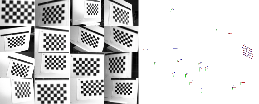
Figure 7: Example of calibration targets acquired for distances between $775$ and $400$ $\mathrm{mm}$ from the checkerboard used in the dataset R12-B, and their respective poses in 3D.

To validate our camera model, we evaluate our method on real-world data obtained with a multi-focus plenoptic camera in a controlled environment. Our experimental setup is illustrated in Figure 1. The camera is mounted on a linear motion table with micro-metric precision. The target plane is orthogonal to the translation axis, and the camera optical axis is aligned with this axis. The approximate absolute distances at which the images have been taken with the corresponding step lengths are reported in Table 1.

6.1 Hardware environment

For our experiments we used a Raytrix R12 color 3D-light-field-camera, with a MLA of F/2.4 aperture. The camera is in Galilean internal configuration. We used two different mounted lens, a Nikon AF Nikkor F/1.8D with a $50\text{\,}\mathrm{mm}$ focal length for comparison with state-of-the-art, and a Nikon AF DC-Nikkor F/2D with a $135\text{\,}\mathrm{mm}$ focal length to validate the generalization of our model. The MLA organization is hexagonal row-aligned, and composed of $176\times 152$ (width $\times$ height) micro-lenses with $I=3$ different types. The sensor is a Basler beA4000-62KC with a pixel size of $s=0.0055$ $\mathrm{mm}$. The raw image resolution is $4080\times 3068~{}$\mathrm{p}\mathrm{i}\mathrm{x}\mathrm{e}\mathrm{l}$$. We calibrate our camera for four focus distance configurations, with $h\in\left\{450,1000,\infty\right\}$ $\mathrm{mm}$ for the $50\text{\,}\mathrm{mm}$ lens, and with $h=1500~{}$\mathrm{mm}$$ for the $135\text{\,}\mathrm{mm}$ lens. Note that when changing the focus setting, the main lens moves with respect to the block MLA-sensor.

6.2 Software environment

All images have been acquired using the MultiCamStudio free software (v6.15.1.3573) of the Euresys company. We set the shutter speed to $5$ $\mathrm{m}\mathrm{s}$. While taking white images for the pre-calibration step, we set the gain to its maximum value. For Raytrix data, we use their proprietary software RxLive (v4.0.50.2) to calibrate the camera, and compute the depth maps used in the evaluation. Our source code has been made publicly available: https://github.com/comsee-research/libpleno, and https://github.com/comsee-research/compote.

Table 1: Summary of R12-A,B,C,D, and UPC-S datasets contents. All distances are given in $\mathrm{mm}$. Scale refers to checkerboard square size. Evaluation distances refer to the linear motion table setup.

		Target		Calib. dist.		Eval. dist.
	$h$	size	scale	min	max	min	max	step
A	450	$9\times 5$	10	175	400	265	385	10
B	1000	$8\times 5$	20	400	775	450	900	50
C	$\infty$	$6\times 4$	30	500	2500	400	1250	50
D	1500	$5\times 3$	20	850	1300	750	1200	50
S	hyperf.	$9\times 6$	26.25	250	800	200	500	50

6.3 Datasets

We build four datasets with different focus distance $h$: for the $50\text{\,}\mathrm{mm}$ lens, R12-A for $h=450~{}$\mathrm{mm}$$, R12-B for $h=1000~{}$\mathrm{mm}$$, and R12-C for $h=\infty$; for the $135\text{\,}\mathrm{mm}$ lens, R12-D for $h=1500~{}$\mathrm{mm}$$. Each dataset is composed of:

• white raw plenoptic images acquired at different apertures ($N\in\left\{4,5.66,8,11.31,16\right\}$) using a light diffuser mounted on the main objective for pre-calibration,

• free-hand calibration target images acquired at various poses (in distance and orientation), separated into two subsets, one for the calibration process ($16$ images) and the other for reprojection error evaluation ($15$ images),

• a white raw plenoptic image acquired in the same luminosity condition and with the same aperture as in the calibration targets acquisition for devignetting,

• and, calibration targets acquired with a controlled translation motion for quantitative evaluation, along with the depth maps computed by the RxLive software.

Examples of calibration targets acquired for the R12-B dataset are given in Figure 7 along with their 3D poses. A summary for each dataset is given in Table 1, indicating checkerboard information and the distances at which the targets have been acquired for calibration and for the controlled evaluation. Our datasets have been made publicly available, and can be downloaded from our public repository at https://github.com/comsee-research/plenoptic-datasets.

6.4 Simulation environment

In order to validate our model on Lytro-like plenoptic camera configuration, i.e., unfocused plenoptic camera (UPC), we propose to evaluate our model in a simulation environment. We built our own simulator based on raytracing to generate images. Similar to the real-world dataset, we generated a dataset, named UPC-S, composed of several white images taken at different apertures (with $N\in\left\{2,4,5.6\right\}$), various checkerboard poses for calibration and validation, and for evaluation, checkerboard images with known translation along the $z$-axis. Details are also given in Table 1. We used the Lytro Illum intrinsic parameters reported in Table 4 of Bok2017 (3) as baseline for the simulation. They have been converted into our parameters and reported in Table 3. The MLA organization is hexagonal row-aligned, and composed of $541\times 434$ (width $\times$ height) micro-lenses of the same type ($I=1$). The raw image resolution is $7728\times 5368~{}$\mathrm{p}\mathrm{i}\mathrm{x}\mathrm{e}\mathrm{l}$$, with a pixel size of $s=0.0014~{}$\mathrm{mm}$$ and with micro-image of radius $7.172\text{\,}\mathrm{p}\mathrm{i}\mathrm{x}\mathrm{e}\mathrm{l}$.

7 Results and Discussions

Our evaluation process follows the steps given in the overview (Figure 2). First, we present the pre-calibration results, where white raw plenoptic images are used for computing micro-image centers, and for estimating initial camera parameters. Second, from the set of devignetted calibration target images, BAP features are extracted, and camera intrinsic and extrinsic parameters are then computed using our non-linear optimization process. In parallel, the same BAP features are also used to calibrate the relative blur proportionality coefficient. Third, we evaluate our model quantitatively, firstly, using the reprojection error as a metric, and secondly, using the relative translation error in a controlled environment. Then, we propose an ablation study of the camera parameters. Finally, we illustrate how to characterize the plenoptic camera extended DoF using the blur profile.

7.1 Pre-calibration

To estimate the parameters $\Omega$, we set $\alpha=2.357$, and since the camera is in Galilean internal configuration, we use $R=-\mathsf{\varrho}\cdot s$,  following Eq. (25). Figure 5 shows the micro-image radii as function of the inverse $f$-number with the estimated lines for dataset R12-B. Their distributions are represented by the violin-boxes. For $N=5.66$, we can see that radii distributions overlap, and that radii values are slightly overestimated as they do not fit exactly the borders of the micro-images. In practice, we only use white images that present distinguishable radii distributions in the estimation process, usually corresponding to small apertures. In case of R12-B, only white images at $N=11.31$ and $N=8$ are used. The corresponding coefficients for all datasets are summarized in Table 2. As expected, the parameter $m$ is different for each dataset, since $D$ and $\Delta_{i}$ vary with the focus distance $h$, whereas the $q^{\prime}_{i}$ values are close for all datasets, even for different camera setup (R12-D).

Table 2: Set of parameters $\Omega$ (in $\mathrm{\SIUnitSymbolMicro m}$) computed during the pre-calibration step for each dataset, along with the calibrated relative blur proportionality coefficient.

	R12-A	R12-B	R12-C	R12-D
$\Delta_{i}$	$128.221\text{\,}631\text{\,}892\text{\,}887\text{\,}07$	$128.293\text{\,}456\text{\,}954\text{\,}452\text{\,}07$	$128.333$	$127.851\text{\,}412\text{\,}062\text{\,}555\text{\,}4$
$\lambda$	0.99441	0.99358	0.99380	0.99746
$m$	$-140.595\text{\,}540\text{\,}404\text{\,}319\text{\,}76$	$-159.561\text{\,}991\text{\,}691\text{\,}589\text{\,}36$	$-155.975\text{\,}446\text{\,}105\text{\,}003\text{\,}36$	$-171.288\text{\,}133\text{\,}405\text{\,}225\text{\,}36$
$q^{\prime}_{1}$	$35.135\text{\,}191\text{\,}355$	$036.489\text{\,}007\text{\,}285\text{\,}581\text{\,}368$	$035.442\text{\,}640\text{\,}815\text{\,}322\text{\,}377$	$038.599\text{\,}053\text{\,}413\text{\,}465\text{\,}3$
$q^{\prime}_{2}$	$40.268\text{\,}205\text{\,}527\text{\,}646\text{\,}997$	$042.074\text{\,}592\text{\,}075\text{\,}095\text{\,}91$	$041.277\text{\,}697\text{\,}120\text{\,}254\text{\,}017$	$043.129\text{\,}202\text{\,}376\text{\,}221\text{\,}407$
$q^{\prime}_{3}$	$36.822\text{\,}146\text{\,}226\text{\,}151\text{\,}445$	$038.806\text{\,}929\text{\,}475\text{\,}413\text{\,}102$	$037.858\text{\,}320\text{\,}210\text{\,}521\text{\,}199$	$040.787\text{\,}991\text{\,}420\text{\,}297\text{\,}272$
$\kappa$	$0.698\text{\,}831\text{\,}500\text{\,}430\text{\,}878\text{\,}94$	$0.698\text{\,}946\text{\,}223\text{\,}507\text{\,}964\text{\,}87$	$0.653\text{\,}121\text{\,}725\text{\,}454\text{\,}249\text{\,}4$	$0.882\text{\,}447\text{\,}646\text{\,}140\text{\,}332\text{\,}44$

7.2 Free-hand camera calibration

Table 3: Initial intrinsic parameters for each dataset along with the optimized parameters obtained by our method (BAP) and with the methods of Noury2017b (30) (NOUR), of Nousias2017 (31) for each micro-lens type (NOUS1, NOUS2, NOUS3) and the parameters obtained from RxLive software (RTRX). Reference and initial intrinsic parameters for the simulated Lytro dataset UPC-S along with the optimized parameters obtained by our method (BAP).

	R12-A  ($F=50~{}$\mathrm{mm}$\text{, }h=450~{}$\mathrm{mm}$$)							R12-B  ($F=50~{}$\mathrm{mm}$\text{, }h=1000~{}$\mathrm{mm}$$)
	Init.	BAP	NOUR	NOUS1	NOUS2	NOUS3	RTRX	Init.	BAP	NOUR	NOUS1	NOUS2	NOUS3	RTRX
$F$ [$\mathrm{mm}$]	$50$	$49.714\text{\,}480$	$54.887\text{\,}986\text{\,}6$	$61.305\text{\,}354\text{\,}7$	$62.476\text{\,}432\text{\,}4$	$63.328\text{\,}32$	$47.709$	$50$	$50.047\text{\,}121\text{\,}936\text{\,}1$	$51.262\text{\,}198\text{\,}50$	$53.912\text{\,}862\text{\,}472\text{\,}9$	$52.987\text{\,}548\text{\,}740\text{\,}521\text{\,}2$	$52.977\text{\,}281\text{\,}94$	$50.8942$
$Q_{1}$ [$\times 10^{-5}$]	0	$24.657\text{\,}25$	$6.098\text{\,}537$	-	-	-	-	0	$2.899\text{\,}517\text{\,}03$	$0.022\text{\,}713\text{\,}011\text{\,}013$	-	-	-	-
$-Q_{2}$ [$\times 10^{-6}$]	0	$2.998\text{\,}39$	$0.925\text{\,}168$	-	-	-	-	0	$0.299\text{\,}757\text{\,}477$	$0.093\text{\,}002\text{\,}22$	-	-	-	-
$Q_{3}$ [$\times 10^{-8}$]	0	$1.0628$	$0.303\text{\,}302\text{\,}7$	-	-	-	-	0	$0.063\text{\,}525\text{\,}983\text{\,}7$	$0.006\text{\,}504\text{\,}398\text{\,}4$	-	-	-	-
$P_{1}$ [$\times 10^{-5}$]	0	$-14.585\text{\,}25$	$-15.027\text{\,}97$	-	-	-	-	0	$14.133\text{\,}984\text{\,}070$	$12.142\text{\,}952$	-	-	-	-
$-P_{2}$ [$\times 10^{-5}$]	0	$6.340\text{\,}192$	$5.019\text{\,}85$	-	-	-	-	0	$21.538\text{\,}891\text{\,}172$	$18.164\text{\,}420\text{\,}950\text{\,}336\text{\,}738$	-	-	-	-
$D$ [$\mathrm{mm}$]	$56.6576$	$56.700\text{\,}741$	$62.4249$	$71.130\text{\,}62$	$72.540\text{\,}80$	$73.530\text{\,}18$	-	$52.1127$	$52.124\text{\,}834\text{\,}510$	$53.296\text{\,}254\text{\,}614\text{\,}647\text{\,}317$	$56.062\text{\,}045\text{\,}65$	$55.127\text{\,}971\text{\,}477\text{\,}0$	$55.124\text{\,}361\text{\,}579\text{\,}0$	-
$-t_{x}$ [$\mathrm{mm}$]	$11.2926$	$10.974\text{\,}348\text{\,}7$	$9.771\text{\,}212$	-	-	-	-	$11.2987$	$12.438\text{\,}356\text{\,}3$	$12.671\text{\,}744\text{\,}569\text{\,}515\text{\,}548$	-	-	-	-
$-t_{y}$ [$\mathrm{mm}$]	$8.4106$	$7.887\text{\,}169$	$8.334\text{\,}331\text{\,}07$	-	-	-	-	$8.416\text{\,}03$	$5.988\text{\,}136\text{\,}336$	$6.113\text{\,}925\text{\,}765\text{\,}874\text{\,}321\text{\,}3$	-	-	-	-
$-\theta_{x}$ [$\mathrm{\SIUnitSymbolMicro rad}$]	0	$843.1$	$468.6$	-	-	-	-	0	$607.2$	$576.2$	-	-	-	-
$\theta_{y}$ [$\mathrm{\SIUnitSymbolMicro rad}$]	0	$637.1$	$321.8$	-	-	-	-	0	$514.5$	$350.4$	-	-	-	-
$\theta_{z}$ [$\mathrm{\SIUnitSymbolMicro rad}$]	$0.552\text{\,}769\text{\,}601\text{\,}998\text{\,}199$	$31.5$	$25.3$	-	-	-	$41.874\text{\,}24$	$016.989\text{\,}042\text{\,}435\text{\,}233\text{\,}1$	$46.0$	$35.3$	-	-	-	$41.874\text{\,}24$
$\Delta_{\mu}$ [$\mathrm{\SIUnitSymbolMicro m}$]	$127.505$	$127.455\text{\,}29$	$127.381\text{\,}16$	-	-	-	$127.357\text{\,}684$	$127.47$	$127.454\text{\,}102$	$127.403\text{\,}475\text{\,}410\text{\,}809\text{\,}15$	-	-	-	$127.357\text{\,}684$
$f{}^{\left(1\right)}$ [$\mathrm{\SIUnitSymbolMicro m}$]	$578.154$	$578.182\text{\,}089\text{\,}885\text{\,}138\text{\,}7$	-	-	-	-	-	$581.102$	$580.489\text{\,}071$	-	-	-	-	-
$f{}^{\left(2\right)}$ [$\mathrm{\SIUnitSymbolMicro m}$]	$504.456$	$505.416\text{\,}411\text{\,}849\text{\,}773\text{\,}04$	-	-	-	-	-	$503.958$	$504.314\text{\,}777\text{\,}752\text{\,}33$	-	-	-	-	-
$f{}^{\left(3\right)}$ [$\mathrm{\SIUnitSymbolMicro m}$]	$551.667$	$552.079\text{\,}041\text{\,}044\text{\,}199$	-	-	-	-	-	$546.393$	$546.356\text{\,}989\text{\,}382\text{\,}8$	-	-	-	-	-
$u_{0}$ [$\mathrm{p}\mathrm{i}\mathrm{x}$]	$2039$	$2070.9$	$2289.8$	$1984.9$	$2034.5$	$1973.7$	-	$2039$	$1958.3$	$1934.9$	$2074.7$	$2094.7$	$1837.0$	-
$v_{0}$ [$\mathrm{p}\mathrm{i}\mathrm{x}$]	$1533$	$1610.9$	$1528.2$	$1482.1$	$1481.0$	$1495.2$	-	$1533$	$1802.9$	$1759.3$	$1640.2$	$1649.1$	$1620.4$	-
$d$ [$\mathrm{\SIUnitSymbolMicro m}$]	$318.632$	$324.774\text{\,}361$	$402.323\text{\,}545$	-	-	-	-	$336.842$	$336.384\text{\,}159$	$363.173\text{\,}728$	-	-	-	-
$d{}^{\left(1\right)}$ [$\mathrm{\SIUnitSymbolMicro m}$]	-	-	-	$585.155\text{\,}936\text{\,}09$	-	-	$407.806\text{\,}128\text{\,}263\text{\,}474$	-	-	-	$447.809\text{\,}603$	-	-	$407.806\text{\,}128\text{\,}263\text{\,}474$
$d{}^{\left(2\right)}$ [$\mathrm{\SIUnitSymbolMicro m}$]	-	-	-	-	$527.586\text{\,}032\text{\,}8$	-	$405.997\text{\,}127\text{\,}294\text{\,}54$	-	-	-	-	$401.925\text{\,}880\text{\,}3$	-	$405.997\text{\,}127\text{\,}294\text{\,}54$
$d{}^{\left(3\right)}$ [$\mathrm{\SIUnitSymbolMicro m}$]	-	-	-	-	-	$561.934\text{\,}508\text{\,}097\text{\,}700\text{\,}2$	$406.895\text{\,}726\text{\,}919\text{\,}174$	-	-	-	-	-	$414.317\text{\,}239\text{\,}6$	$406.895\text{\,}726\text{\,}919\text{\,}174$

	R12-C  ($F=50~{}$\mathrm{mm}$\text{, }h=\infty$)							R12-D		UPC-S
	Init.	BAP	NOUR	NOUS1	NOUS2	NOUS3	RTRX	Init.	BAP	Ref.	Init.	BAP
$F$ [$\mathrm{mm}$]	$50$	$50.013\text{\,}031\text{\,}225\text{\,}428\text{\,}279$	$53.321\text{\,}663\text{\,}056\text{\,}716\text{\,}744$	$51.113\text{\,}120\text{\,}433\text{\,}796\text{\,}82$	$49.918\text{\,}849\text{\,}892\text{\,}113\text{\,}53$	$50.812\text{\,}403\text{\,}039\text{\,}675\text{\,}32$	$51.5635$	$135$	$136.105\text{\,}166\text{\,}709\text{\,}309\text{\,}77$	$9.984\text{\,}45$	$10$	$10.229\text{\,}728\text{\,}755\text{\,}768\text{\,}972$
$Q_{1}$ [$\times 10^{-5}$]	0	$18.613\text{\,}490\text{\,}5$	$1.392\text{\,}717\text{\,}953\text{\,}835\text{\,}163\text{\,}6$	-	-	-	-	0	$35.974\text{\,}498\text{\,}894\text{\,}915\text{\,}505$	0	0	-$7.913\text{\,}287\text{\,}829\text{\,}9$
$-Q_{2}$ [$\times 10^{-6}$]	0	$2.646\text{\,}232\text{\,}48$	$0.382\text{\,}050\text{\,}407\text{\,}916\text{\,}851\text{\,}6$	-	-	-	-	0	$8.083\text{\,}212\text{\,}390\text{\,}028\text{\,}945$	0	0	-$3.881\text{\,}930\text{\,}7$
$Q_{3}$ [$\times 10^{-8}$]	0	$1.037\text{\,}642\text{\,}409\text{\,}6$	$0.104\text{\,}056\text{\,}463\text{\,}361\text{\,}118\text{\,}67$	-	-	-	-	0	$4.820\text{\,}932\text{\,}981\text{\,}690\text{\,}617$	0	0	-$5.821\text{\,}374\text{\,}4$
$P_{1}$ [$\times 10^{-5}$]	0	$19.109\text{\,}101\text{\,}367\text{\,}79$	$27.719\text{\,}919\text{\,}106\text{\,}678\text{\,}484$	-	-	-	-	0	$-4.311\text{\,}638\text{\,}562\text{\,}539\text{\,}256\text{\,}5$	0	0	-$3.5767$
$-P_{2}$ [$\times 10^{-5}$]	0	$7.310\text{\,}573\text{\,}137\text{\,}75$	$4.460\text{\,}704\text{\,}410\text{\,}342\text{\,}737\text{\,}3$	-	-	-	-	0	$-3.758\text{\,}200\text{\,}100\text{\,}808\text{\,}535\text{\,}3$	0	0	$0.116\text{\,}994\text{\,}898$
$D$ [$\mathrm{mm}$]	$49.3841$	$49.361\text{\,}607\text{\,}994\text{\,}7$	$52.378\text{\,}980\text{\,}888\text{\,}444\text{\,}85$	$50.331\text{\,}351\text{\,}663\text{\,}385\text{\,}84$	$49.066\text{\,}959\text{\,}360\text{\,}055\text{\,}54$	$49.882\text{\,}201\text{\,}543\text{\,}617\text{\,}41$	-	$149.242\text{\,}563\text{\,}551\text{\,}545$	$149.104\text{\,}604\text{\,}938\text{\,}429\text{\,}36$	$9.847\text{\,}916\text{\,}429$	$10$	$10.005\text{\,}486\text{\,}613\text{\,}307\text{\,}905$
$-t_{x}$ [$\mathrm{mm}$]	$11.261\text{\,}763\text{\,}581\text{\,}600\text{\,}288$	$13.125\text{\,}022\text{\,}314\text{\,}02$	$14.158\text{\,}858\text{\,}382\text{\,}582\text{\,}752$	-	-	-	-	$11.2987$	$11.208\text{\,}316\text{\,}218\text{\,}108\text{\,}749$	$5.459\text{\,}28$	$5.404\text{\,}700\text{\,}000\text{\,}000\text{\,}000\text{\,}1$	0
$-t_{y}$ [$\mathrm{mm}$]	$8.417\text{\,}81$	$7.445\text{\,}715\text{\,}535\text{\,}802\text{\,}826$	$6.230\text{\,}845\text{\,}978\text{\,}950\text{\,}848\text{\,}8$	-	-	-	-	$8.386\text{\,}582\text{\,}845\text{\,}615\text{\,}764\text{\,}7$	$8.350\text{\,}873\text{\,}683\text{\,}089\text{\,}268\text{\,}7$	$3.7179$	$3.747\text{\,}800\text{\,}000\text{\,}000\text{\,}000\text{\,}2$	0
$-\theta_{x}$ [$\mathrm{\SIUnitSymbolMicro rad}$]	0	$490.9$	$487.7$	-	-	-	-	0	$371.119\text{\,}471\text{\,}185\text{\,}201\text{\,}42$	0	0	-$0.529\text{\,}552\text{\,}6$
$\theta_{y}$ [$\mathrm{\SIUnitSymbolMicro rad}$]	0	$388.9$	$366.1$	-	-	-	-	0	$287.047\text{\,}413\text{\,}591\text{\,}936\text{\,}6$	0	0	$0.943\text{\,}843\text{\,}87$
$\theta_{z}$ [$\mathrm{\SIUnitSymbolMicro rad}$]	$027.961\text{\,}214\text{\,}821\text{\,}336\text{\,}5$	$41.1$	$49.1$	-	-	-	$36.629\text{\,}038\text{\,}401\text{\,}7$	$5.794\text{\,}623\text{\,}978\text{\,}840\text{\,}437$	$35.445\text{\,}740\text{\,}626\text{\,}310\text{\,}149$	0	0	-$0.033\text{\,}267\text{\,}277\text{\,}564\text{\,}5$
$\Delta_{\mu}$ [$\mathrm{\SIUnitSymbolMicro m}$]	$127.537$	$127.484\text{\,}224\text{\,}811\text{\,}56$	$127.417\text{\,}561\text{\,}372\text{\,}069\text{\,}19$	-	-	-	$127.357\text{\,}684$	$127.527\text{\,}797\text{\,}272\text{\,}155\text{\,}02$	$127.509\text{\,}351\text{\,}109\text{\,}389\text{\,}1$	$20$	$19.986\text{\,}916\text{\,}170\text{\,}727\text{\,}197$	$19.986\text{\,}878\text{\,}364\text{\,}538\text{\,}083$
$f{}^{\left(1\right)}$ [$\mathrm{\SIUnitSymbolMicro m}$]	$554.348$	$569.878\text{\,}578\text{\,}597$	-	-	-	-	-	$625.625\text{\,}457\text{\,}769\text{\,}698\text{\,}02$	$636.063\text{\,}493\text{\,}736\text{\,}291\text{\,}45$	$40.087\text{\,}372$	$47.753\text{\,}07$	$47.747\text{\,}450\text{\,}736\text{\,}751\text{\,}49$
$f{}^{\left(2\right)}$ [$\mathrm{\SIUnitSymbolMicro m}$]	$475.984$	$491.712\text{\,}040\text{\,}342\text{\,}29$	-	-	-	-	-	$559.911\text{\,}826\text{\,}113\text{\,}209$	$572.518\text{\,}093\text{\,}914\text{\,}525\text{\,}24$	-	-	-
$f{}^{\left(3\right)}$ [$\mathrm{\SIUnitSymbolMicro m}$]	$518.976$	$535.283\text{\,}887\text{\,}725\text{\,}89$	-	-	-	-	-	$592.050\text{\,}493\text{\,}794\text{\,}584\text{\,}63$	$604.227\text{\,}014\text{\,}410\text{\,}881\text{\,}45$	-	-	-
$u_{0}$ [$\mathrm{p}\mathrm{i}\mathrm{x}$]	$2039$	$1692.1$	$2131.6$	$1966.3$	$1913.8$	$2052.5$	-	$2039$	$2028.7$	$3842.8$	$3863$	$3861.7$
$v_{0}$ [$\mathrm{p}\mathrm{i}\mathrm{x}$]	$1533$	$1677.8$	$1445.9$	$1484.6$	$1487.2$	$1492.7$	-	$1533$	$1526.7$	$2719.5$	$2683$	$2715.5$
$d$ [$\mathrm{\SIUnitSymbolMicro m}$]	$307.929$	$319.527\text{\,}769$	$367.402\text{\,}085$	-	-	-	-	$378.718\text{\,}224\text{\,}227\text{\,}469\text{\,}59$	$382.304\text{\,}332\text{\,}869\text{\,}068\text{\,}73$	$40.087\text{\,}372$	$47.2792$	$47.322\text{\,}794\text{\,}127\text{\,}719\text{\,}447$
$d{}^{\left(1\right)}$ [$\mathrm{\SIUnitSymbolMicro m}$]	-	-	-	$357.795\text{\,}271\text{\,}442\text{\,}7$	-	-	$407.806\text{\,}128\text{\,}263\text{\,}474$	-	-	-	-	-
$d{}^{\left(2\right)}$ [$\mathrm{\SIUnitSymbolMicro m}$]	-	-	-	-	$349.994\text{\,}830\text{\,}282\text{\,}0$	-	$405.997\text{\,}127\text{\,}294\text{\,}54$	-	-	-	-	-
$d{}^{\left(3\right)}$ [$\mathrm{\SIUnitSymbolMicro m}$]	-	-	-	-	-	$353.264\text{\,}214\text{\,}36$	$406.895\text{\,}726\text{\,}919\text{\,}174$	-	-	-	-	-

Comparison with state-of-the-art.

Since our model is close to the one of Noury2017b (30), we compare our intrinsics with the ones obtained under their pinhole assumption using only corner reprojection error and with the same initial parameters. In addition, we evaluate against the method of Nousias2017 (31), which provides a set of intrinsics and extrinsics for each micro-lens type. The equivalence of our parameters and their parameters is given by

$$F =\frac{(f_{x}+f_{y})}{2}\cdot s\text{, } D=-F\cdot\left(\frac{K_{1}}{K_{2}}\cdot F+1\right)^{-1}\text{, }$$ ((42))

$$d{}^{\left(i\right)} =D-\frac{K_{2}D}{D+K_{2}}\text{, } u_{0}=c_{x}~{}~{}\text{ and }~{}~{}v_{0}=c_{y}\text{, }$$

where $K_{1}$ and $K_{2}$ are the two additional intrinsic parameters that account for the MLA setting in their model. The equivalence also stands for the parameters of Bok2017 (3). The provided detector from Nousias2017 (31) was not able to detect corner observations on our datasets. Therefore, we used the same observations for our method (noted BAP in Table 3), Noury2017b (30) method (NOUR), and Nousias2017 (31) method for each type (NOUS1, NOUS2, and NOUS3), which allowed us to focus the comparison on the camera model only. Finally, we provide the calibration parameters obtained from the RxLive software (RTRX) corresponding to the model of Heinze2016b (16), and compare our depth measurements to their depth maps.

Initialization.

We initialize $\lambda$ from Eq. (28). Its value for each dataset is reported in Table 2. The difference between the initial value of $\lambda$ and its value computed from optimized camera parameter is less than $0.024\text{\,}\mathrm{\char 37\relax}$, which validates the use of the initial value from Eq. (28) when computing our BAP features. The initial camera parameters reported in Table 3 are computed using the methodology presented in subsection 3.3. They are used for the BAP and NOUR methods. The camera internal configuration is set to Galilean. When $h$ decreases, $D$ increases. Yet when the main lens focus distance is at infinity, the main lens should focus on the plane $\upsilon=2$, which implies that $D$ tends to $F-2d$ as lower bound, as $H$ tends to $F$. In most cases (here, for R12-A,B,D), we will still have $F<D$, which usually can describe the camera in Keplerian configuration. In Keplerian internal configuration, the condition $F<D$ stands regardless of the focus distance, as $D$ lower bound is $F+2d$.

When using the linear initialization from NOUS, the initial parameters of some configurations corresponded to impossible physical setup or were too far from the solution, hindering the convergence of the optimization. Therefore, in order to continue comparison, we manually set the initial parameters close enough to a solution. In contrast, we can see that the optimized parameters for BAP and NOUR are close to initial values, which shows that our pre-calibration step provides a strong initial solution for the optimization process.

Intrinsic camera parameters.

Optimized intrinsic parameters are reported for each dataset and for all the evaluated methods in Table 3. First, BAP, NOUR and NOUS all verify the condition $F\approx D+2d$ when the focus is set at infinity (R12-C). Second, the focal lengths obtained from NOUR, NOUS and RTRX change significantly given the focus distance, and the ones obtained from NOUS even vary according to the micro-lens types. In contrast, only BAP shows stable parameters across all three R12-A,B,C datasets. Shared parameters across datasets (i.e., the focal lengths and the distance between the MLA and the sensor) are close enough to indicate that our model successfully generalizes to different focus configurations. Furthermore, the parameters obtained by our method with an other main lens, i.e., R12-D, are coherent with the previously obtained parameters, stressing out that our model can be applied to a different camera setting. Finally, our method is the only one providing the micro-lenses focal lengths in a single unified model. The other methods calibrate either several MLA-sensor distances (RTRX), or several models, one for each type (NOUS).

Note that distortion coefficients and MLA rotations are close to zero. The influence of these parameters will be analyzed in the proposed ablation study of the camera model in subsection 7.4.

On simulated data.

First, pre-calibration has been performed using the white raw images. The resulting parameters $\Omega$ are coherent with the simulation parameters. With parameters $m=$-23.639\text{\,}\mathrm{\SIUnitSymbolMicro m}$$ and $q=$-0.146\text{\,}\mathrm{\SIUnitSymbolMicro m}$$, we have $d\approx f$, which describes the unfocused configuration. Reference and initial intrinsic parameters are reported in Table 3, along with the optimized parameters. Second, calibration has been performed. The obtained intrinsic parameters are close enough to the references parameters, indicating that our method is able to generalize to the unfocused plenoptic camera.
For completeness, we also quantitatively evaluated the optimized parameters, by estimating the relative displacement between checkerboard with known motion along the $z$-axis. It results a translation error $\varepsilon_{z}=$1.64\text{\,}\mathrm{\char 37\relax}$$, which validates the model.

7.3 Quantitative evaluations of the camera model

Reprojection error.

In the absence of ground truth, we first evaluated the intrinsic parameters by estimating the reprojection error using the previously computed intrinsics. We consider only free-hand calibration target images which are not used in the calibration process. We use the root-mean-square error (RMSE) as a metric to evaluate the reprojection error on the corner part of the features, for each dataset. For the BAP method, the corner reprojection part is reported in Table 4, as well as the radius reprojection part within parentheses. Regarding the NOUS methods, the original error is expressed using the mean reprojection error (MRE). We converted the final error to the RMSE metric for comparison. Note that the latter method operates separately on each type of micro-lens, meaning that the number of features is not the same as with NOUR and BAP. First, the reprojection error is less than $1\text{\,}\mathrm{p}\mathrm{i}\mathrm{x}\mathrm{e}\mathrm{l}$ for all methods, for each dataset, demonstrating that the computed intrinsics lead to an accurate reprojection model and can be generalized to images which are not from the calibration set. Second, even though the NOUS method provides the lowest RMSE, it shows a significant discrepancy according to the considered type. The error obtained by our method is sightly higher than the error from NOUR, but this can be explained by the fact that our optimization does not aim at minimizing only the corner reprojection error, but the radius reprojection as well. Note that the positional error $\epsilon_{u,v}$ predominates in the total cost by two orders of magnitude compared to the blur radius error $\epsilon_{\rho}$, but the latter still helps to constrain our model as shown by the relatively close intrinsics between the datasets.

Controlled environment poses evaluation.

With our experimental setup, we acquired several images with known relative translation between each frame. We compare the estimated displacements along the $z$-axis from the extrinsic parameters to the ground truth. The extrinsics are computed with the models estimated from the free-hand calibration. In the case of the RTRX method, we use the filtered depth maps obtained with the proprietary software RxLive to estimate the displacements.

Figure 8: Translation error along the $z$-axis with respect to the ground truth displacement from the closest frame, for datasets R12-A (a), R12-B (b) and R12-C (c). The error $\varepsilon_{z}$ is expressed in percentage of the estimated distances, and truncated to $7\text{\,}\mathrm{\char 37\relax}$ to ease the readability and the comparison. The mean error with its confidence interval across all datasets for our method (BAP), Noury2017b (30) method (NOUR), Nousias2017 (31) method for each type (NOUS1, NOUS2, NOUS3), and for the proprietary software RxLive (RTRX) are reported in (d). Please refer to the color version for better visualization.

The translation errors along the $z$-axis with respect to the ground truth displacement from the closest frame are reported in Figure 8 for datasets R12-A (a), R12-B (b) and R12-C (c). The relative error $\varepsilon_{z}$ for a known displacement $\delta_{z}$ is computed as the mean absolute relative difference between the estimated displacement $\hat{\delta_{z}}$ and the ground truth, for each pair of frames $\left(\bm{T}_{i},\bm{T}_{j}\right)$ separated by a distance $\delta_{z}$, i.e.,

$$\mathrm{\varepsilon_{z}}\!\left(\delta_{z}\right)=\eta^{-1}\sum_{\left(\bm{T}_{i},\bm{T}_{j}\right)\mid z_{i}-z_{j}=\delta_{z}}{\left|\delta_{z}-\hat{\delta_{z}}\right|}\textfractionsolidus{\delta_{z}}\text{, }$$ ((43))

where $\hat{\delta_{z}}=\hat{z_{i}}-\hat{z_{j}}$, and $\eta$ is a normalization constant corresponding to the number of frames pair. The mean error with its standard deviation across all datasets for BAP, NOUR, NOUS, and RTRX are reported in (d).

Table 4: Corner reprojection error for each evaluation dataset (i.e., free-hand calibration target images not part of the calibration dataset) using the RMSE metric. For the BAP method, reprojection error of the radius part is indicated within parentheses.

	BAP	NOUR	NOUS1	NOUS2	NOUS3
R12-A	$0.856\text{\,}418$ ($0.082\text{\,}619\text{\,}8$)	$0.712\text{\,}565$	$0.772\text{\,}922\text{\,}125\text{\,}085\text{\,}144\text{\,}1$	0.667	$0.958\text{\,}257\text{\,}890\text{\,}324\text{\,}191\text{\,}4$
R12-B	$0.673\text{\,}851$ ($0.183\text{\,}383$)	$0.617\text{\,}605$	$0.537\text{\,}975\text{\,}177\text{\,}589\text{\,}917\text{\,}6$	0.519	$0.593\text{\,}133\text{\,}593\text{\,}487\text{\,}832\text{\,}9$
R12-C	$0.737\text{\,}945$ ($0.040\text{\,}595\text{\,}4$)	$0.712\text{\,}565$	$1.287\text{\,}158\text{\,}262\text{\,}915\text{\,}446$	$0.681\text{\,}368\text{\,}136\text{\,}700\text{\,}311\text{\,}9$	0.411

Firstly, the mean error across R12-A,B,C datasets are of the same order for the evaluated methods around $3\text{\,}\mathrm{\char 37\relax}$: for BAP, $\varepsilon_{z}=2.92\pm 0.73~{}$\mathrm{\char 37\relax}$$; for NOUR, $\varepsilon_{z}=3.50\pm 3.08~{}$\mathrm{\char 37\relax}$$; for NOUS1, $\varepsilon_{z}=1.68\pm 1.53~{}$\mathrm{\char 37\relax}$$; for NOUS2, $\varepsilon_{z}=3.40\pm 2.19~{}$\mathrm{\char 37\relax}$$; for NOUS3, $\varepsilon_{z}=3.30\pm 3.35~{}$\mathrm{\char 37\relax}$$; and, for RTRX, $\varepsilon_{z}=4.96\pm 4.44~{}$\mathrm{\char 37\relax}$$. This is also the case for the dataset R12-D where our model has a mean translation error of $\varepsilon_{z}=3.37~{}$\mathrm{\char 37\relax}$$. Note that all evaluated methods outperform RTRX as the depth maps computation might not be as precise as the optimization of extrinsic parameters. Our method ranks second in terms of relative mean error. Even though lowest error is obtained by the method NOUS for type $(1)$, it presents a large standard deviation and the errors for the other two types are significantly higher. In real application context, there is no way to know in advance which type will produce the smallest error. Nousias2017 (31) suggest that when extrinsics are sufficiently close, we can use representative extrinsics that are calculated by averaging the extrinsics from the individual types. Our results do not match this observation as the estimated extrinsics are significantly different for each type. As shown, only the first type gives satisfactory results whereas the other two present a larger error with a significant standard deviation. Averaging the extrinsics from all types will therefore minimize the difference between poses but will not provide the best possible estimation.

Secondly, the standard deviation can be seen as an indicator of the estimation precision across the datasets, and thus indicates whether the model can generalize to several configurations or not. Our model presents the lowest standard deviation as illustrated in Figure 8 (d). This indicates a low discrepancy between datasets and thus that the model is precise and consistent for all configurations.

Thirdly, we analyze the behavior of each method for each dataset across different distances. None of the methods suffered from a constant bias, as we do not observe a decreasing relative error as the distance increases. BAP and NOUR present a stable relative error for all distances, i.e., with approximately $0.3\text{\,}\mathrm{\char 37\relax}$ of standard deviation. This indicates that the estimation suffered only from a scale error. One could thus re-scale the poses to provide a precise and accurate estimation. We cannot draw any conclusion for the other methods since the variations do not follow any obvious pattern.

Finally, our model differs from the model of Noury2017b (30) by modeling the micro-lens focal lengths. Comparing those two models, the mean error as well as the standard deviation is smaller with our method. The inclusion of the micro-lens focal lengths in the camera model improves the estimation precision and accuracy, and enables to generalize to several configurations. Dealing with different intrinsics which produce different extrinsics is not satisfactory when using the multi-focus plenoptic camera. In contrast, our model is able to manage all micro-lens types simultaneously, and proves to be stable across various configurations and working distances.

7.4 Ablation study of camera parameters

To evaluate the influence of each parameter of the camera model, we present an ablation study of some of them. We focus the analysis on distortion coefficients ($Q_{1}$, $Q_{2}$, $Q_{3}$, $P_{1}$, and $P_{2}$), on some degrees of freedom of the MLA, especially its tilt with respect to the sensor ($\theta_{x},\theta_{y}$), and the pitch between micro-lenses ($\Delta_{\mu}$). All combinations of the parameters have been tested, resulting in eight configurations. For each configuration and on each dataset of R12-A,B,C: first, we calibrate the camera intrinsic parameters; second, we evaluate the model using the RMSE of the reprojection error; and finally, we quantitatively estimate the relative translation error on the evaluation dataset. Each configuration has been initialized with the same intrinsic parameters, and used the same observations for all processes. Results are reported in Table 5. The first column is the configuration number. The Tilt column indicates if we keep (✓) or remove ($\times$) the parameters $\theta_{x}$ and $\theta_{y}$. The Pitch column stands for the parameter $\Delta_{\mu}$, and the column Dist for the distortion parameters $Q_{1}$, $Q_{2}$, $Q_{3}$, $P_{1}$, and $P_{2}$. The reprojection error ${\epsilon_{all}}$ is given by its RMSE, and the relative translation error ${\epsilon_{z}}$ is expressed in percent with respect to the ground truth displacement.

Table 5: Ablation study of some camera parameters. For each dataset, the reprojection error ${\epsilon_{all}}$, computed using the RMSE along with the relative translation error ${\epsilon_{z}}$, expressed in $\mathrm{\char 37\relax}$, are reported. The symbol ✓(resp., $\times$) indicates if we keep (resp., remove) the considered parameters.

	Tilt	Pitch	Dist	R12-A		R12-B		R12-C
				${\epsilon_{all}}$	${\epsilon_{z}}$	${\epsilon_{all}}$	${\epsilon_{z}}$	${\epsilon_{all}}$	${\epsilon_{z}}$
1	✓	✓	✓	0.860	3.23	0.698	3.15	$0.738\text{\,}684\text{\,}029$	$2.310\text{\,}381\text{\,}13$
2	✓	✓	$\times$	$0.866\text{\,}422\text{\,}07$	$3.338\text{\,}91$	$0.700\text{\,}050\text{\,}924$	$3.197\text{\,}026$	0.737	$3.184\text{\,}292\text{\,}57$
3	✓	$\times$	✓	$0.884\text{\,}110\text{\,}041$	$3.876\text{\,}323$	$0.755\text{\,}160\text{\,}051$	$3.211\text{\,}813\text{\,}422\text{\,}6$	$0.770\text{\,}359\text{\,}045$	2.00
4	✓	$\times$	$\times$	$0.891\text{\,}059\text{\,}207$	$3.976\text{\,}911\text{\,}865$	$0.751\text{\,}962\text{\,}488$	$3.235\text{\,}505\text{\,}357$	$0.772\text{\,}731\text{\,}93$	$3.133\text{\,}764\text{\,}226$
5	$\times$	✓	✓	$0.864\text{\,}695\text{\,}193$	$3.483\text{\,}333$	$0.784\text{\,}339\text{\,}725$	3.15	$0.759\text{\,}739\text{\,}712$	$2.894\text{\,}325\text{\,}984$
6	$\times$	✓	$\times$	$0.863\text{\,}570\text{\,}87$	$3.580\text{\,}493\text{\,}77$	$0.716\text{\,}440\text{\,}9$	$3.156\text{\,}086\text{\,}31$	$0.748\text{\,}509\text{\,}444$	$3.042\text{\,}542\text{\,}619$
7	$\times$	$\times$	✓	-	-	-	-	-	-
8	$\times$	$\times$	$\times$	-	-	-	-	-	-

The configuration $1$ is our reference, corresponding to the complete model. The optimized parameters are close to the ones from Table 3, i.e., with less than $1\text{\,}\mathrm{\char 37\relax}$ of variation, for all converging configurations and for all datasets.

First, the distortions do not impact the reprojection error of the model. Considering the pairs of configurations $\left(1,2\right)$, $\left(3,4\right)$, and $\left(5,6\right)$, the errors are similar with or without distortions, indicating that our camera does not suffer from lateral distortions. This is due to the relatively large main lens focal length. Nevertheless, distortions may have a role to play in case of shorter focal length.

Second, removing the rotations of the MLA does not improve nor worsen the reprojection error and the pose estimation. When keeping the tilt but freezing the pitch, the model is able to converge. The tilt, in combination with other factors (such as a slight decrease of the main lens focal length), compensates for the error introduced by the approximate value of the pitch. In contrast, configurations $7$ and $8$ do not converge to a solution, showing that when removing both the tilt and the pitch of the MLA, the model is not constrained enough, and the reprojection error cannot be minimized, resulting in a failure.

Finally, when freezing the pitch to its initial value, the positional part of the reprojection error increases. It is especially the case for dataset R12-A, where the reported errors in Table 5 are the highest of all configurations. This confirms our previous observation that the deviation of the micro-image centers and their optical centers does not satisfy an orthographic projection between the MIA and the MLA. The pitch should be taken into account, on one hand to improve the precision of the model, and on the other hand not to hinder the optimization process.

7.5 Relative blur calibration

We calibrate the blur proportionality coefficient $\kappa$ for the three datasets using our BAP features. Figure 9 presents two windows extracted around BAP features of different types from the same cluster, showing different amount of blur. The target image to be equally-defocused according to our model is shown before, (b), and after, (c), blur addition. The estimated PSF of the relative blur is given in (d).

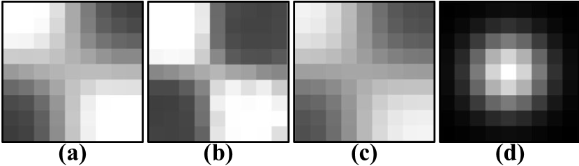
Figure 9: (a) Reference image with highest amount of blur. (b) Target image to be equally-defocused. (c) Target image with additional blur. (d) Estimated point-spread function (PSF).

The optimized blur proportionality coefficients $\kappa$ are reported in Table 3. Theoretically, the parameter should be the same for all three datasets. Empirically this observation is validated for R12-A and R12-B. Estimated $\kappa$ for R12-C is lower. This is because the micro-lenses focal lengths in R12-C are slightly shorter than in R12-A and R12-B. Analytically, this difference generates a higher amount of relative blur, and thus a shorter estimate of $\kappa$ to match the observed blur in image space. In other words, $\kappa$ compensates for the slight differences in $f{}^{\left(i\right)}$ estimates. Therefore, $\kappa$ should be calibrated for each dataset.

7.6 Profiling the plenoptic camera

Using the parameters from our calibration process, we plot the blur profile of the camera, i.e., the evolution of the blur radius with respect to depth for each micro-lens type along with its corresponding DoF. Figure 10 shows the blur profiles obtained for our three focus distance configurations, with their DoFs expressed in $\mathrm{mm}$. The blur radius is expressed in pixel and is given for each type, in red for type $(1)$, in green for type $(2)$ and in blue for type $(3)$. Distances are given in object space in $\mathrm{mm}$ with their corresponding virtual depth on a secondary $x$-axis, spanning from $\upsilon=1$ to $15$, except for the configuration $h=\infty$ where we cropped just after the farthest focal plane. In MLA space, the profiles have the same behavior for all focus distances, as it only depends on the MLA parameters.

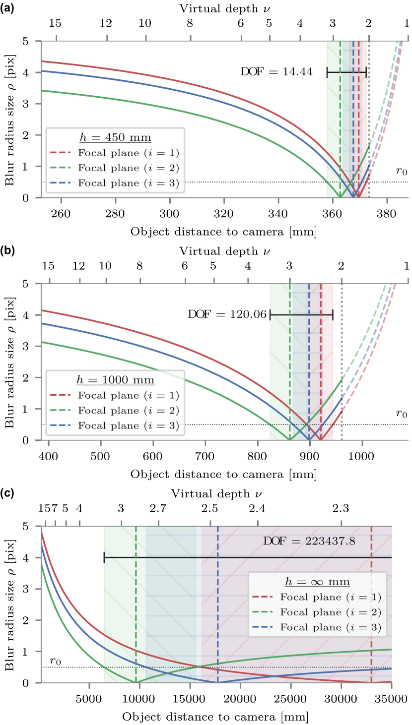
Figure 10: Blur profile, including each micro-lens type, in object space, at different focus distances: (a) $h=450~{}$\mathrm{mm}$$; (b) $h=1000~{}$\mathrm{mm}$$; and (c) $h=\infty~{}$\mathrm{mm}$$. Focal planes and depth of fields are illustrated for each type. The blur radius is expressed in $\mathrm{p}\mathrm{i}\mathrm{x}\mathrm{e}\mathrm{l}$ as function of the object distance to the camera in $\mathrm{mm}$. Corresponding virtual depth is reported on the secondary $x$-axis.

First, the horizontal dashed line represents the radius of the minimal acceptable circle of confusion $r_{0}$. In our case, at a wavelength of $750\text{\,}\mathrm{nm}$, the radius of the smallest diffraction-limited spot is $r^{*}=2.4~{}$\mathrm{\SIUnitSymbolMicro m}$$ which is less than half the pixel size. We then choose $r_{0}=s/2$. Despite not illustrated in the figure, the blur radius grows exponentially when getting closer to the plane $\upsilon=0$. Once this limit is exceeded, the blur decreases and converges to a constant value of approximately $6\text{\,}\mathrm{p}\mathrm{i}\mathrm{x}\mathrm{e}\mathrm{l}$. This happens for more distant objects when points are projected in front of MLA implying a negative virtual depth. This is the case for $h=450$ and $h=1000~{}$\mathrm{mm}$$, but not for $h=\infty$, as the points were never projected closer than $\upsilon=2$. In the working distance range, the blur does not exceed $5\text{\,}\mathrm{p}\mathrm{i}\mathrm{x}\mathrm{e}\mathrm{l}$ and grows when points are closer to the camera.

Secondly, we can use the DoF to select the range of working distances where the blur is not noticeable. The DoF increases in object space as the focus distance increases. As reported on the figures: for R12-A, the DoF is of $14.44~{}$\mathrm{mm}$$; for R12-B of $120~{}$\mathrm{mm}$$; and finally, for R12-C, the total DoF is of $223~{}$\mathrm{m}$$. In MLA space the total DoF is constant and spans from $\upsilon=2.15$ to $3.45$. As expected, the DoFs overlap. In particular, the DoF of the type $(3)$ micro-lens is entirely included in the other two, whereas the DoFs of the type $(1)$ and $(2)$ just touch. Within the total DoF, a point can then be seen focused in two micro-images of different types simultaneously, which eases the matching problem between views.

Finally, we can easily identify the distance limits at which the point will not be in the DoF anymore nor be projected on multiple micro-images, i.e., corresponding to virtual distances $\left|\upsilon\right|<2$. At these distances, disparity cannot be computed in image space, and no depth estimation can be performed. Such estimation can also be hindered by the resolution in virtual space compared to the resolution in object space as disparity is inversely proportional to virtual depth. For instance, for close objects, points will be projected on more micro-images but with a low disparity. So the profiles can be used to efficiently characterize the range of distances according to the desired application. Furthermore, once the MLA parameters are available, we can simulate an approximate blur profile for the desired focus distance $h$ with the desired main lens focal length $F$ by updating the value of $D$ using Eq. (26) and Eq. (27).

8 Conclusion

To calibrate a plenoptic camera, state-of-the-art methods rely on simplifying hypotheses, on reconstructed data or require separate calibration processes to take into account the multi-focus configuration. Taking advantage of blur information we propose: 1) a more complete plenoptic camera model with the introduction of a new BAP feature that explicitly models the defocus blur; this new feature is exploited in our calibration process based on non-linear optimization of reprojection errors; 2) a new relative blur calibration to fill the gap between the physical and geometric blur, which enables us to fully exploit blur in image space; and 3) a way to profile the plenoptic camera and its extended depth of field (DoF).

Our camera model is applicable to the multi-focus plenoptic camera (both in Galilean and Keplerian configuration), as well as to the single-focus and unfocused plenoptic camera. In case of the Raytrix multi-focus camera, our ablation study shows that main lens distortions and MLA tilt can be omitted without hindering the calibration process nor the pose estimation. The study also indicates that explicitly including the pitch of the micro-lenses in the model improves the results. In addition, our calibration methods are validated by quantitative evaluations in controlled environment on real-world data. Our method provides strong initial intrinsics during the pre-calibration step, and coherent optimized camera parameters for all evaluated configurations. It shows a low and stable relative translation error across all the datasets.

In the future, we plan to use blur information in complement to disparity to improve metric depth estimation.

Declarations

Data Availability Statement

The datasets analyzed for this study can be found in the following repository: https://github.com/comsee-research/plenoptic-datasets. All data supporting the results of this paper will be provided upon request.

Code availability Statement

The code source has been made open-source and publicly available in the following repositories: https://github.com/comsee-research/libpleno, and https://github.com/comsee-research/compote.

Conflict of Interest Statement

The authors declare that the research was conducted in the absence of any commercial or financial relationships that could be construed as a potential conflict of interest.

References

- (1) Tom E. Bishop and Paolo Favaro “The Light Field Camera : Extended Depth of Field, Aliasing, and Superresolution” In IEEE Transactions on Pattern Analysis and Machine Intelligence 34.5, 2012, pp. 972–986 DOI: 10.1109/TPAMI.2011.168
- (2) Yunsu Bok, Hae-Gon Jeon and In So Kweon “Geometric Calibration of Micro-Lens-Based Light-Field Cameras Using Line Features” In Computer Vision – ECCV 2014 Springer International Publishing, 2014, pp. 47–61 DOI: 10.1007/978-3-319-10599-4“˙4
- (3) Yunsu Bok, Hae-Gon Jeon and In So Kweon “Geometric Calibration of Micro-Lens-Based Light Field Cameras Using Line Features” In IEEE Transactions on Pattern Analysis and Machine Intelligence 39.2, 2017, pp. 287–300 DOI: 10.1109/TPAMI.2016.2541145
- (4) Duane Brown “Decentering Distortion of Lenses - The Prism Effect Encountered in Metric Cameras can be Overcome Through Analytic Calibration” In Photometric Engineering 32.3, 1966, pp. 444–462
- (5) Ching Hui Chen, Hui Zhou and Timo Ahonen “Blur-aware disparity estimation from defocus stereo images” In Proceedings of the IEEE International Conference on Computer Vision 2015 Inter, 2015, pp. 855–863 DOI: 10.1109/ICCV.2015.104
- (6) Ae Conrady “Decentered Lens-Systems” In Monthly Notices of the Royal Astronomical Soceity 79, 1919, pp. 384–390 DOI: 10.1093/mnras/79.5.384
- (7) Donald G. Dansereau, Oscar Pizarro and Stefan B. Williams “Decoding, calibration and rectification for lenselet-based plenoptic cameras” In Proceedings of the IEEE Computer Society Conference on Computer Vision and Pattern Recognition, 2013, pp. 1027–1034 DOI: 10.1109/CVPR.2013.137
- (8) John Ens and Peter Lawrence “An Investigation of Methods for Determining Depth from Focus” In IEEE Transactions on Pattern Analysis and Machine Intelligence 15.2, 1993, pp. 97–108 DOI: 10.1109/34.192482
- (9) Martin Ester, Hans-Peter Kriegel, Jiirg Sander and Xiaowei Xu “A Density-Based Algorithm for Discovering Clusters in Large Spatial Databases with Noise” In KDD, 1996
- (10) Todor Georgiev et al. “Spatio-Angular Resolution Tradeoff in Integral Photography” In Rendering Techniques 2006.263-272, 2006, pp. 21 DOI: 10.2312/EGWR/EGSR06/263-272
- (11) Todor Georgiev and Andrew Lumsdaine “Depth of Field in Plenoptic Cameras” In Eurographics 2009, 2009, pp. 5–8 DOI: 10.2312/egs.20091035
- (12) Todor Georgiev and Andrew Lumsdaine “Resolution in Plenoptic Cameras” In Frontiers in Optics 2009/Laser Science XXV/Fall 2009 OSA Optics & Photonics Technical Digest, 2009, pp. CTuB3 DOI: 10.1364/COSI.2009.CTuB3
- (13) Todor Georgiev and Andrew Lumsdaine “The multifocus plenoptic camera” In Digital Photography VIII SPIE, 2012, pp. 69–79 International Society for OpticsPhotonics DOI: 10.1117/12.908667
- (14) Michael D. Grossberg and Shree K. Nayar “The raxel imaging model and ray-based calibration” In International Journal of Computer Vision 61.2, 2005, pp. 119–137 DOI: 10.1023/B:VISI.0000043754.56350.10
- (15) Christopher Hahne et al. “Baseline and Triangulation Geometry in a Standard Plenoptic Camera” In International Journal of Computer Vision 126.1, 2018, pp. 21–35 DOI: 10.1007/s11263-017-1036-4
- (16) Christian Heinze, Stefano Spyropoulos, Stephan Hussmann and Christian Perwaß “Automated Robust Metric Calibration Algorithm for Multifocus Plenoptic Cameras” In IEEE Transactions on Instrumentation and Measurement 65.5, 2016, pp. 1197–1205
- (17) Ole Johannsen, Christian Heinze, Bastian Goldluecke and Christian Perwaß “On the calibration of focused plenoptic cameras” In Lecture Notes in Computer Science (including subseries Lecture Notes in Artificial Intelligence and Lecture Notes in Bioinformatics) 8200 LNCS, 2013, pp. 302–317 DOI: 10.1007/978-3-642-44964-2“˙15
- (18) Ole Johannsen et al. “A Taxonomy and Evaluation of Dense Light Field Depth Estimation Algorithms” In IEEE Computer Society Conference on Computer Vision and Pattern Recognition Workshops 2017-July, 2017, pp. 1795–1812 DOI: 10.1109/CVPRW.2017.226
- (19) Laurent Kneip, Davide Scaramuzza and Roland Siegwart “A novel parametrization of the perspective-three-point problem for a direct computation of absolute camera position and orientation” In Proceedings of the IEEE Computer Society Conference on Computer Vision and Pattern Recognition, 2011, pp. 2969–2976 DOI: 10.1109/CVPR.2011.5995464
- (20) Mathieu Labussière, Céline Teulière, Frédéric Bernardin and Omar Ait-Aider “Blur Aware Calibration of Multi-Focus Plenoptic Camera” In 2020 IEEE/CVF Conference on Computer Vision and Pattern Recognition (CVPR) IEEE, 2020, pp. 2542–2551 DOI: 10.1109/CVPR42600.2020.00262
- (21) Anat Levin, William T. Freeman and Frédo Durand “Understanding camera trade-offs through a Bayesian analysis of light field projections” In Lecture Notes in Computer Science (including subseries Lecture Notes in Artificial Intelligence and Lecture Notes in Bioinformatics) 5305 LNCS.PART 4, 2008, pp. 88–101 DOI: 10.1007/978-3-540-88693-8-7
- (22) Marc Levoy and Pat Hanrahan “Light field rendering” In Proceedings of the 23rd annual conference on Computer graphics and interactive techniques - SIGGRAPH ’96 New York, New York, USA: ACM Press, 1996, pp. 31–42 DOI: 10.1145/237170.237199
- (23) Gabriel Lippmann “Integral Photography” In Academy of the Sciences, 1911 DOI: 10.1017/CBO9781107415324.004
- (24) Andrew Lumsdaine and Todor Georgiev “The focused plenoptic camera” In IEEE International Conference on Computational Photography (ICCP), 2009, pp. 1–8 DOI: 10.1109/ICCPHOT.2009.5559008
- (25) Fahim Mannan and Michael S. Langer “Blur calibration for depth from defocus” In 13th Conference on Computer and Robot Vision (CRV), 2016, pp. 281–288 DOI: 10.1109/CRV.2016.62
- (26) Fahim Mannan and Michael S. Langer “What is a good model for depth from defocus?” In 13th Conference on Computer and Robot Vision (CRV), 2016, pp. 273–280 DOI: 10.1109/CRV.2016.61
- (27) Lois Mignard-Debise, John Restrepo and Ivo Ihrke “A Unifying First-Order Model for Light-Field Cameras: The Equivalent Camera Array” In IEEE Transactions on Computational Imaging 3.4, 2017, pp. 798–810 DOI: 10.1109/TCI.2017.2699427
- (28) Ren Ng et al. “Light Field Photography with a Hand-held Plenoptic Camera”, 2005, pp. 1–11 DOI: 10.1.1.163.488
- (29) Charles-antoine Noury “Etalonnage de caméra plénoptique et estimation de profondeur à partir des données brutes”, 2019
- (30) Charles Antoine Noury, Céline Teulière and Michel Dhome “Light-Field Camera Calibration from Raw Images” In DICTA 2017 – International Conference on Digital Image Computing: Techniques and Applications, 2017, pp. 1–8 DOI: 10.1109/DICTA.2017.8227459
- (31) Sotiris Nousias et al. “Corner-Based Geometric Calibration of Multi-focus Plenoptic Cameras” In Proceedings of the IEEE International Conference on Computer Vision, 2017, pp. 957–965 DOI: 10.1109/ICCV.2017.109
- (32) Sean O’Brien, Jochen Trumpf, Viorela Ila and Robert Mahony “Calibrating light-field cameras using plenoptic disc features” In 2018 International Conference on 3D Vision (3DV) IEEE, 2018, pp. 286–294 DOI: 10.1109/3DV.2018.00041
- (33) Luca Palmieri and Reinhard Koch “Optimizing the Lens Selection Process for Multi-focus Plenoptic Cameras and Numerical Evaluation” In IEEE Computer Society Conference on Computer Vision and Pattern Recognition Workshops 2017-July, 2017, pp. 1763–1774 DOI: 10.1109/CVPRW.2017.223
- (34) Alex Paul Pentland “A New Sense for Depth of Field” In IEEE Transactions on Pattern Analysis and Machine Intelligence PAMI-9.4, 1987, pp. 523–531 DOI: 10.1109/TPAMI.1987.4767940
- (35) Christian Perwaß and Lennart Wietzke “Single Lens 3D-Camera with Extended Depth-of-Field” In Human Vision and Electronic Imaging XVII 49.431 SPIE, 2012, pp. 829108 DOI: 10.1117/12.909882
- (36) Shengxian Shi et al. “Parametric study on light field volumetric particle image velocimetry” In Flow Measurement and Instrumentation 49 Elsevier, 2016, pp. 70–88 DOI: 10.1016/j.flowmeasinst.2016.05.006
- (37) Klaus H. Strobl and Martin Lingenauber “Stepwise calibration of focused plenoptic cameras” In Computer Vision and Image Understanding 145 Elsevier Inc., 2016, pp. 140–147 DOI: 10.1016/j.cviu.2015.12.010
- (38) M. Subbarao “Parallel Depth Recovery By Changing Camera Parameters”, 1988, pp. 149–155 DOI: 10.1109/ccv.1988.589986
- (39) Murali Subbarao “Determining Distance from Defocused Images of Simple Objects” In 89-07-20, 1989, pp. 11794–12350
- (40) Murali Subbarao and Gopal Surya “Depth from defocus: A spatial domain approach” In International Journal of Computer Vision 13.3, 1994, pp. 271–294 DOI: 10.1007/BF02028349
- (41) Piotr Suliga and Tomasz Wrona “Microlens array calibration method for a light field camera” In Proceedings of the 19th International Carpathian Control Conference (ICCC) IEEE, 2018, pp. 19–22 DOI: 10.1109/CarpathianCC.2018.8399595
- (42) Chelsea M. Thomason, Brian S. Thurow and Timothy W. Fahringer “Calibration of a Microlens Array for a Plenoptic Camera” In 52nd Aerospace Sciences Meeting, 2014, pp. 1–18 DOI: 10.2514/6.2014-0396
- (43) Yuan Wang et al. “Virtual Image Points Based Geometrical Parameters’ Calibration for Focused Light Field Camera” In IEEE Access 6.c, 2018, pp. 71317–71326 DOI: 10.1109/ACCESS.2018.2881990
- (44) Niclas Zeller, Franz Quint and Uwe Stilla “Calibration and accuracy analysis of a focused plenoptic camera” In ISPRS Annals of Photogrammetry, Remote Sensing and Spatial Information Sciences II-3.September, 2014, pp. 205–212 DOI: 10.5194/isprsannals-II-3-205-2014
- (45) Niclas Zeller, Franz Quint, Marcel Sutterlin and Uwe Stilla “Investigating mathematical models for focused plenoptic cameras” In 2016 12th IEEE International Symposium on Electronics and Telecommunications (ISETC) IEEE, 2016, pp. 301–304 DOI: 10.1109/ISETC.2016.7781117
- (46) Niclas Zeller et al. “Metric Calibration of a Focused Plenoptic Camera based on a 3D Calibration Target” In ISPRS Annals of Photogrammetry, Remote Sensing and Spatial Information Sciences III-3.July, 2016, pp. 449–456 DOI: 10.5194/isprs-annals-III-3-449-2016
- (47) Niclas Zeller, Franz Quint and Uwe Stilla “From the Calibration of a Light-Field Camera to Direct Plenoptic Odometry” In IEEE Journal of Selected Topics in Signal Processing 11.7, 2017, pp. 1004–1019 DOI: 10.1109/JSTSP.2017.2737965
- (48) Chunping Zhang, Zhe Ji and Qing Wang “Unconstrained Two-parallel-plane Model for Focused Plenoptic Cameras Calibration”, 2016, pp. 1–20 arXiv:1608.04509
- (49) Qi Zhang et al. “A Generic Multi-Projection-Center Model and Calibration Method for Light Field Cameras” In IEEE Transactions on Pattern Analysis and Machine Intelligence, 2018 DOI: 10.1109/TPAMI.2018.2864617
- (50) Yuanyuan Zhao, Haotian Li, Di Mei and Shengxian Shi “Metric calibration of unfocused plenoptic cameras for three-dimensional shape measurement” In Optical Engineering 59.07, 2020, pp. 1 DOI: 10.1117/1.oe.59.7.073104
- (51) Ping Zhou et al. “A two-step calibration method of lenslet-based light field cameras” In Optics and Lasers in Engineering 115 Elsevier Ltd, 2019, pp. 190–196 DOI: 10.1016/j.optlaseng.2018.11.024