Probing Transit Timing Variations of Three Hot-Jupiters: HATP-36b, HATP-56b, and WASP-52b

Abstract

We report the results of new transit observations for the three hot Jupiter-like planets HATP-36b, HATP-56b and WASP-52b respectively. Transit timing variations (TTVs) are presented for these systems based on observations that span the period 2016 - 2020. The data were collected with the 0.6 m telescope at Adiyaman University (ADYU60, Turkey) and the 1.0 m telescope at TÜBİTAK National Observatory (TUG, Turkey). Global fits were performed to the combined light curves for each system along with the corresponding radial velocity (RV) data taken from the literature. The extracted parameters (for all three systems) are found to be consistent with the values from previous studies. Through fits to the combined mid-transit times data from our observations and the data available in the literature, an updated linear ephemeris is obtained for each system. Although a number of potential outliers are noted in the respective O-C diagrams, the majority of the data are consistent within the 3$\sigma$ confidence level implying a lack of convincing evidence for the existence of additional objects in the systems studied.

1 Introduction

Since the discovery of the first hot Jupiter-like exoplanet (Mayor & Queloz, 1995) several thousand exoplanets ($\sim$ 4375) have been confirmed, the majority of which ($\sim$ 3354) have been detected using the transit method. The light curves measured by the transit method not only verify or improve the parameters of the system, but also provide important information about the presence of additional objects in the system via the long-term transit time variations (TTVs; Agol et al. (2005)).

Discovered by the HATNet Exoplanet survey (Bakos et al., 2004), HATP-36b, is a transiting hot-Jupiter (1.832M_J, 1.264R_J) orbiting around a V = 12.5 mag, G5V type Sun-like star (1.022M_⊙, 1.096R_⊙). This system has a short orbital period of 1.33 days (Bakos et al., 2012; Mancini et al., 2015). Following the discovery of HATP-36b, Maciejewski et al. (2013) followed the object with photometric observations using a 0.6 m telescope and improved the transit ephemeris. The system has also been studied by Mancini et al. (2015) as part of the GAPS program; the addition of new spectroscopic and photometric data has produced a revised set of physical parameters. The authors also noted anomalies in three photometric transit light curves and confirmed, by the analysis of the HARPS-N spectra, that these were compatible with star spot complexes on the surface of the star. Wang et al. (2019) combined 26 new transit observations for HATP-36b with the ones from the literature and investigated the existence of a third object. Despite the new data set, which covers a relatively long time period, they did not detect significant variations in the transit timing variation (TTV) signal. Chakrabarty & Sengupta (2019) analyzed high-quality photometric data for HATP-36b using a wavelet-based denoising technique to minimize the effects of various background contributions such varying sky transparency and stellar activity. They presented updated results for the transit parameters with higher precision compared to the previous ones.

HATP-56b, also discovered by the HATNet Exoplanet survey (Huang et al., 2015), is an inflated hot-Jupiter exoplanet with the following physical parameters determined by combining ground-based photometric and spectroscopic observations: mass of M_P= 2.18M_J, and a radius of R_P=1.43R_J. It orbits a F-type star with magnitude of V = 10.91 and has an orbital period of 2.7908 days. The maximum rotational period for HatP-56 has been reported as 1.8$\pm$0.2 days based on the spectroscopic measurements (Zhou et al., 2016). In addition, the periodogram of the K2 light curve suggests that the host star in the system is a $\gamma$ Dor variable (Huang et al., 2015). Using Doppler tomographic analyses for the spectroscopic transits, Zhou et al. (2016) reported a spin–orbit aligned (8^o $\pm$ 2^o) geometry for HATP-56b. They also examined a tidal re-alignment model for rapidly rotating host stars similar to HATP-56b and found no evidence that the rotation rates of the system were altered by star–planet tidal interactions. Furthermore, they noted that HATP-56b is a system in which the rotation period of the host star is faster than the orbital period of the planet.

WASP-52b is another planet that falls in the hot-Jupiter category and orbits a Sun-like K2V type star with a mass of 0.87($\pm$ 0.03)M_⊙ and radius of 0.79($\pm$ 0.02)R_⊙. It was first reported by Hebrard et al. (2013). They estimated the physical parameters of the system as; planet mass M_P= 0.46$\pm$0.02M_J, a planetary radius of R_P=1.27$\pm$0.03R_J, and an orbital period of P = 1.7497798 $\pm$ 0.0000012 days. WASP-52 system has been studied by many authors to probe the anomalies seen in the transit light curves (e.g. potential effects due to stellar spots and/or bright regions in the stellar photosphere) (Swift et al., 2015; Baluev et al., 2015; Kirk et al., 2016; Chen et al., 2017; Mancini et al., 2017; Louden et al., 2017; Bruno et al., 2018; Ozturk & Erdem, 2019). A detailed TTV study by Baluev et al. (2015) using the data collected from the literature did not show any indication of a third object in the system. Later studies suggested that the variations seen in the transit times could either be due to existence of a third object in the system or the effect of stellar spots (Mancini et al., 2017; Barros et al., 2013; Oshagh et al., 2013; Ioannidis, Huber & Schmitt, 2016). The TTVs have been investigated with the use of linear and quadratic models; parabolic changes in residuals of the transits have beeen reported by Ozturk & Erdem (2019). In another study (Chen et al., 2017), spectroscopic observations suggest a possible cloudy atmosphere for WASP-52b.

The possibility of detecting additional objects through the study of TTVs, and in particular, the intriguing notion of observing features in the measured light curves that might be attributable to stellar surface activity, provide the primary motivation for this work. In this study, we present the results of new transit observations for the three hot Jupiter-like planets HATP-36b, HATP-56b and WASP-52b respectively; the period of observations spans 2016 - 2020. The paper is organized as follows: in Section 2, we describe the photometric observations and reduction of the data acquired for HATP-36b, HATP-56b and WASP-52b and the details of the computation of the system parameters, and the TTV analysis. The implications of these results are discussed in Section 3. We conclude by summarizing our main findings in Section 4.

2 Observations and Data Reduction

2.1 Photometric Observations

New photometric observations of HATP-36b, HATP-56b and WASP-52b were carried out with 0.6 m and 1 m telescopes. The 0.6 m telescope (ADYU60) is located at Adiyaman University, Turkey and is currently operated remotely from the Adiyaman University Observatory. ADYU60 is equipped with 1k x 1k Andor iKon-M934 CCD with a pixel size and image scale of 13$\mu$m $\times$ 13$\mu$m and 0.67$\arcsec$/pixel respectively. The 1.0 m Ritchey–Chrétien (RC) telescope (T100) is located at the Bakirlitepe Mountain and is currently operated remotely from TUG (TÜBİTAK National Observatory) in Antalya, Turkey. The T100 telescope houses a 4k $\times$ 4k SI 1100 CCD camera operating at -90^∘C. The pixel size, overall field of view and image scale of the CCD camera are 15$\mu$m $\times$ 15$\mu$m, $21.5\arcmin\times 21.5\arcmin$ and 0.31$\arcsec$/pixel respectively. Photometric observations for Adyu60 were made with the $Johnson$ R filter and for T100 we used the $Bessel$ R filter. Defocussing technique was adopted in the T100 observations to improve the statistics of the photometric data for a given exposure time.

We observed a total of sixteen transits for HATP-36b with Adyu60 and one transit with T100 between April 2016 - June 2020. In addition, Adyu60 was used to observe nine transits for HATP-56b between December 2016 - February 2018 and thirteen transits for WASP-52b between August 2016 - October 2020. In order to maintain relatively high signal-to-noise ratios, some exposure times were adjusted based on changing weather conditions and according to the magnitude of the target. However, during all phases of the transits, the exposure was kept fixed to acquire data with consistent time intervals. The summaries of our observations are given in Table 1.

Table 1: Log of observations.

Date of	Object	Telescope	Filter	Exposure (s)	Number of	Airmass	RMS
observations					data points		mmag
01.04.2016	HATP-36b	TUG	R	45	164	1.09 - 1.80	7.042
01.04.2016	HATP-36b	ADYU60	R	120	79	1.13 – 1.76	4.667
11.05.2016	HATP-36b	ADYU60	R	150	38	1.10 – 1.38	2.452
22.01.2017	HATP-36b	ADYU60	R	60	133	1.24 – 1.06	4.728
19.02.2017	HATP-36b	ADYU60	R	90	79	1.53 - 1.01	6.919
23.02.2017	HATP-36b	ADYU60	R	90	87	1.57 – 1.01	6.050
25.04.2017	HATP-36b	ADYU60	R	120	99	1.06 – 1.69	3.335
08.06.2017	HATP-36b	ADYU60	R	120	73	1.01 – 1.21	5.758
30.01.2018	HATP-36b	ADYU60	R	120	123	1.31 – 1.02	6.382
07.02.2018	HATP-36b	ADYU60	R	120	165	1.39 – 1.04	13.329
30.03.2020	HATP-36b	ADYU60	R	120	138	1.61 – 1.01	2.994
10.05.2020	HATP-36b	ADYU60	R	120	119	1.08 – 2.18	6.172
30.05.2020	HATP-36b	ADYU60	R	120	138	1.03 – 2.00	3.541
03.06.2020	HATP-36b	ADYU60	R	120	131	1.02 – 1.87	2.568
07.06.2020	HATP-36b	ADYU60	R	120	111	1.03 – 1.67	5.978
11.06.2020	HATP-36b	ADYU60	R	120	105	1.04 – 1.65	3.980
15.06.2020	HATP-36b	ADYU60	R	120	91	1.05 - 1.57	2.989
08.12.2016	HATP-56b	ADYU60	R	120	128	2.27 - 1.03	2.122
19.01.2017	HATP-56b	ADYU60	R	120	112	2.02 - 1.05	2.353
13.02.2017	HATP-56b	ADYU60	R	120	130	1.05 - 1.35	2.414
27.02.2017	HATP-56b	ADYU60	R	120	107	1.07 - 1.17	2.217
22.10.2017	HATP-56b	ADYU60	R	120	119	1.75 - 1.02	1.950
14.12.2017	HATP-56b	ADYU60	R	120	143	1.02 - 1.90	2.748
28.12.2017	HATP-56b	ADYU60	R	120	115	1.02 - 1.62	6.773
11.01.2018	HATP-56b	ADYU60	R	120	74	1.02 - 1.56	3.825
08.02.2018	HATP-56b	ADYU60	R	120	73	1.02 - 1.03	4.652
12.08.2016	WASP-52b	ADYU60	R	120	82	1.26 - 1.18	2.931
26.08.2016	WASP-52b	ADYU60	R	120	85	1.17 - 1.28	3.505
07.10.2016	WASP-52b	ADYU60	R	120	95	1.23 - 2.8	4.241
22.01.2017	WASP-52b	ADYU60	R	60	57	1.52 - 3.27	13.450
22.09.2017	WASP-52b	ADYU60	R	120	55	1.15 - 1.40	6.421
13.10.2017	WASP-52b	ADYU60	R	120	100	1.16 - 2.05	3.425
20.10.2017	WASP-52b	ADYU60	R	120	90	1.20 - 2.30	4.483
27.10.2017	WASP-52b	ADYU60	R	120	85	1.22 - 2.30	5.092
07.09.2018	WASP-52b	ADYU60	R	120	90	1.41 - 1.17	3.339
14.09.2018	WASP-52b	ADYU60	R	120	90	1.33 - 1.19	3.164
05.10.2018	WASP-52b	ADYU60	R	60	98	1.20 - 1.35	3.294
18.09.2020	WASP-52b	ADYU60	R	120	94	2.17 - 1.16	4.601
02.10.2020	WASP-52b	ADYU60	R	120	96	1.84 - 1.15	6.221

2.2 Data Reduction

The software package, AstroImageJ (AIJ) (Collins et al. 2017), was deployed to perform data reduction, calibrations, extraction of differential aperture photometry and detrending parameters. AIJ is a powerful tool for image processing and precise photometry especially for exoplanet transit light curves. We used median-combined bias and flat frames to correct the raw CCD images by using the Data Processor module of AIJ. Dark correction was not applied because dark counts were negligible in the frames for both telescopes. We performed differential photometry using the Multi-Aperture (MA) module in AIJ. To obtain differential magnitudes for each system, we considered as many comparison stars as we could find in the CCD frames. In the final analysis, we selected two or three comparison stars with the least-variable light curves. The same set of standard stars were used for all observations of a given source. Photometric uncertainties, CCD read-out noise etc., were estimated using MA module of AIJ. The details of the selected comparisons are given in Table 2. In order to minimize the transit modeling residuals, we determined the aperture sizes of the target and comparison stars by using the "radial profile" feature of the AIJ program, and we allowed the aperture sizes to vary by 1.2 times the FWHM value in each image. The conversion from Julian Date (JD) to Barycentric Julian Date (BJD) was done within AIJ. We used AIJ Multi-plot module to extract detrend parameters. These parameters are airmass, time, sky background, FWHM of the average PSF in each image, total comparison star counts, and target x-centroid and y-centroid positions on the detector. These parameters, along with relative flux and corresponding flux errors, were then used to create simultaneous detrended light curves in EXOFASTv2 as part of the global and individual fits for consistency. In EXOFASTv2 we simply include additional columns of detrending parameters for each transit in the transit file to detrend against. We kept the same number of detrend parameters for each source. We used additive detrending scheme of EXOFASTv2 in our analysis. The final light curves were obtained from the differential magnitudes, and for each light curve, the RMS was calculated to obtain a measure of the quality of the data. The RMS varies in the range $\sim(1.9-7.0)$ mmags, primarily reflecting the count rates and the different observing conditions during which the light curves were measured.

Table 2: The information on comparison stars. Magnitudes are taken from the SIMBAD catalog¹.

Object	RA	DEC	Kmag
HATP-36	12 33 03.909	+44 54 55.180	10.603
2MASS 12331133+4451365	12 33 11.339	+44 51 36.550	11.462
2MASS 12331452+4449494	12 33 14.528	+44 49 49.490	12.172
2MASS 12330477+4457439	12 33 04.779	+44 57 43.934	11.288
HATP-56	06 43 23.529	+27 15 08.218	9.830
TYC 1901-762-1	06 43 21.915	+27 16 33.245	11.734
TYC 1901-1083-1	06 43 21.789	+27 17 50.300	11.505
WASP-52	23 13 58.76	+08 45 40.6	10.086
2MASS 23140483+0844176	23 14 05.034	+08 44 19.54	11.883
2MASS 23135436+0848293	23 13 54.44	+08 48 31.48	12.087
${}^{1}{http://simbad.u-strasbg.fr/simbad/}$

2.3 Global Fits

To determine the planetary system parameters, along with their uncertainties, we deployed the Markov Chain Monte Carlo code EXOFASTv2 (Eastman, Gaudi, & Agol, 2013; Eastman, 2017; Eastman et al., 2019). The updated version of the code provides a general solution encompassing a multi-parameter space covering an arbitrary number of light curves along with multiple radial velocity (RV) and SED data sets. The code calculates both the stellar and planetary parameters as well as the transit and limb darkening parameters. EXOFASTv2 uses several different methods to robustly constrain the stellar parameters. In our calculations we set both NOMIST and TORRES keywords to be able to recover the behavior of the original EXOFAST, using the empirical Torres et al. (2010) relations to derive the stellar mass and radius. EXOFASTv2 is capable of fitting a number of astrometric data sets for a number of planets with RV data sets by scaling the RV and light curve uncertainties. In this study, we fit our transit light curves along with published RV data. The HATP-36 RV data were obtained by Bakos et al. (2012) with the Tillinghast Reflector Echelle Spectrograph (TRES) mounted on the 1.5m Fred Lawrence Whipple Observatory (FLWO) telescope; the HATP-56 RV data were taken at the same facility by Huang et al. (2015), and finally, the WASP-52 RV data were obtained by Hebrard et al. (2013) using the CORALIE spectrograph (mounted on the 1.2-m Euler-Swiss telescope at La Silla).

EXOFASTv2 allows the user to supply Gaussian or uniform priors on any fitted or derived parameter. Priors can simply be listed in a configuration file. In our analysis we have listed a set of stellar and planetary prior parameters which are derived from previous studies in the literature. These prior parameters are $T_{\rm eff}$, $[{\rm Fe/H}]$, $R_{*}$, $M_{*}$, linear and quadratic limb darkening coefficients, $R_{P}$, $M_{P}$, eccentricity (if available in the literature), period, inclination, and transit impact parameter. We included their uncertainties in our analysis because fixing values is generally not recommended (Eastman et al., 2019), and avoids under estimating the uncertainties of any covariant parameter.

To perform the global fits, we used the prior system parameters given by Bakos et al. (2012) ($R_{*}$, $M_{*}$,$T_{\rm eff}$,$[{\rm Fe/H}]$, P, $R_{P}$ and $M_{P}$), Wang et al. (2019) (eccentricity) for HATP-36, Huang et al. (2015) ($R_{*}$, $M_{*}$,$T_{\rm eff}$,$[{\rm Fe/H}]$, P, $R_{P}$ and b) for HATP-56, and Hebrard et al. (2013) ($R_{*}$, $M_{*}$,$T_{\rm eff}$,$[{\rm Fe/H}]$, P) for WASP-52. The limb-darkening parameters were taken from the NASA Exoplanet Archive.

The transit and RV data were independently fitted with EXOFAST and the errors scaled to find the maximum likelihood with lowest $\chi^{2}$ for every best-fit model. A global fit was performed using both data sets. The default configuration for the very latest version of EXOFAST (see Eastman et al. (2019)) uses the MIST stellar evolutionary models of Dotter (2016). However, as noted earlier, we opted to use NOMIST and TORRES options during the fitting procedure (Eastman, Gaudi, & Agol, 2013; Eastman, 2017; Eastman et al., 2019) to be consistent with earlier studies. EXOFASTv2 calculates Gelman–Rubin statistic (GR; Gelman & Rubin (1992)) and the number of independent draws of the underlying posterior probability distribution (Tz; Ford (2006)) statistic metrics to judge the convergence. We used default EXOFASTv2 statistics as Tz > 1000 and GR < 1.01 for each parameter to derive the stellar parameters from the global fits. The median values of the posterior distributions for the system parameters, along with the uncertainties (at the $1\sigma$ level), are listed in Tables 3, 4 and 5. The posterior distributions obtained for the main stellar and planetary parameters of each system are presented in the (online) Appendix; see Figures 19, 20 and 21.

2.4 Mid-Transit Times and TTVs

The possible signature of the existence of a third body (or more bodies) ensues from the systematic variation of the mid-transit times of the system (consisting of a star and an exoplanet). To search for TTVs, calculated and measured mid-transit times are needed. The mid-transit time can be calculated from the following expression: $T_{C}=T_{0}+P_{orb}\times L$, where $T_{0}$ is the initial ephemeris time when the cycle is equal to zero, $P_{orb}$ is orbital period, and $L$ is the cycle count with respect to the zeroth (or reference) cycle. To extract the observed mid-transit times, we used EXOFASTv2 to separately obtain best-fits for each light curve of our target systems. In addition to our own data, we obtained the published mid-times from the literature. For each system, the observed and the mid-transit times obtained from the literature (along with their uncertainties), are listed in Tables 6, 8 and 9 respectively.

Using the mid-transit times, we proceeded to obtain the parameters of the linear ephemeris equation by deploying the MCMC affine-invariant ensemble sampler of the emcee package (Goodman & Weare, 2010) implemented by Foreman-Mackey et al. (2013). The priors were taken from calculations based on a linear model using the LMFIT package (Newville et al., 2016) by minimizing chi-square. To determine the best-fit parameters of the linear ephemeris model and posterior probability distributions, we used a likelihood function ($\mathcal{L}$) as in Goździewski et al. (2015):

$$\ln{\mathcal{L}}=-\frac{1}{2}\sum_{i}^{N}\chi^{2}-\sum_{i}^{N}\ln{\sqrt{\sigma_{i}^{2}+\sigma_{f}^{2}}}-N\ln{\sqrt{2\pi}}$$ (1)

where the $\chi^{2}$ function is given by

$$\chi^{2}=\frac{(O-C)_{i}^{2}}{\sigma_{i}^{2}+\sigma_{f}^{2}}$$ (2)

Here, $(O-C)_{i}$ denotes the difference between $i$th observed and calculated ephemeris time, and $\sigma_{i}$ is the uncertainty in the observed $i$th ephemeris. This form of $\mathcal{L}$ allows the determination of the free parameter $\sigma_{f}$ (sometimes called the fractional amount) that scales the raw uncertainties $\sigma_{i}$ in quadrature (Goodman & Weare, 2010; Goździewski et al., 2015). During sampling the range for the priors of the parameters $T_{0},P_{orb},\sigma_{f}$ was set to be $>0$ days. Then, we performed MCMC for 512 initial walkers (for 30,000 steps), thus providing an effective MCMC chain for the calculation. The resulting 1-D and 2-D posterior probability distributions of the parameters describing the ephemeris (for each system under study) were recorded.

3 Results and Discussion

3.1 System Parameters

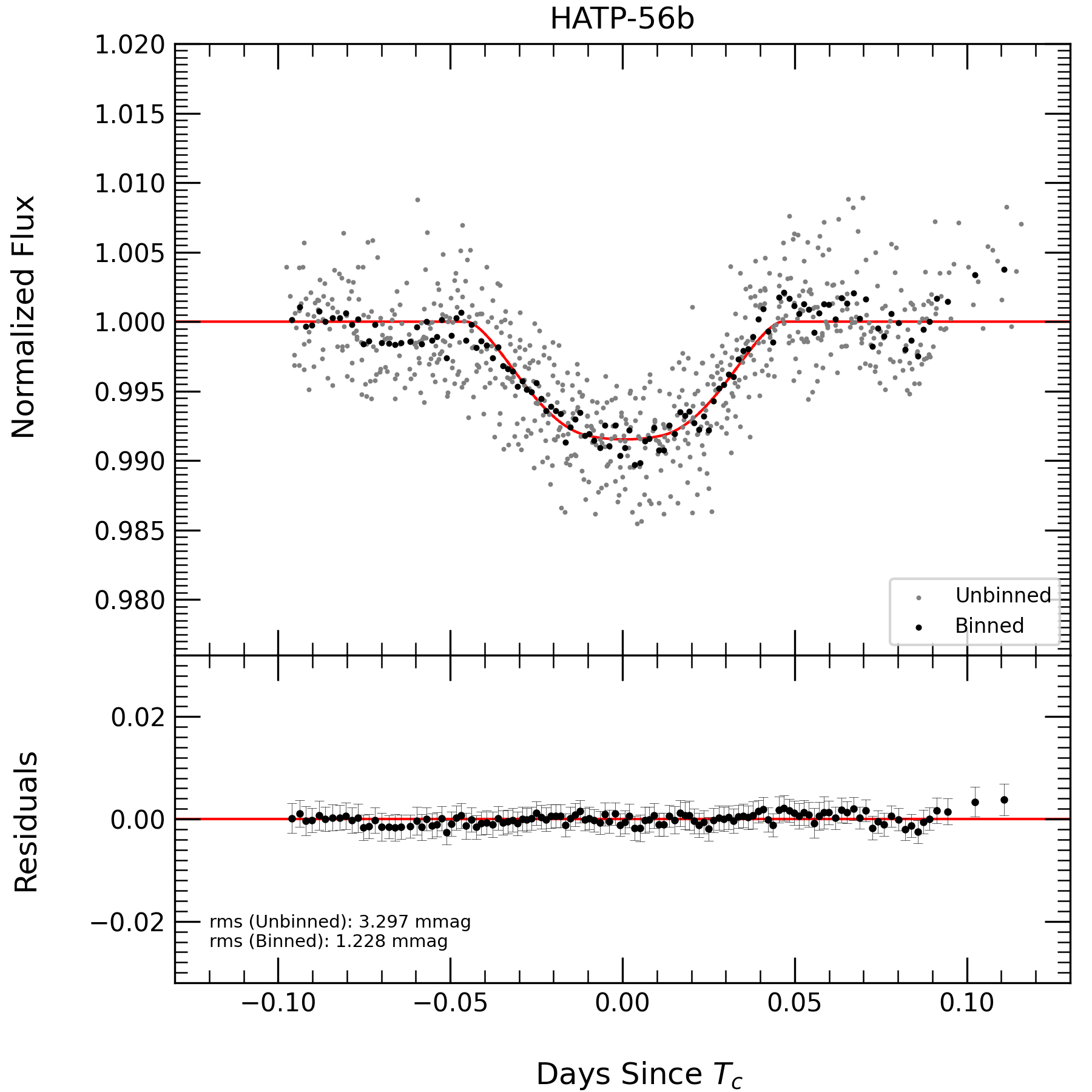
Figure 7: The fitted transit light curves of HATP-56b are shown in the top panel. Unbinned transit light curves are shown as grey points. Binned transit light curves shown as black points. Model residuals for binned transit light curves (for black points) shown in the bottom panel. The RMS of the binned data is $\sim$ 1.2 mmag and the binning is 147 s.

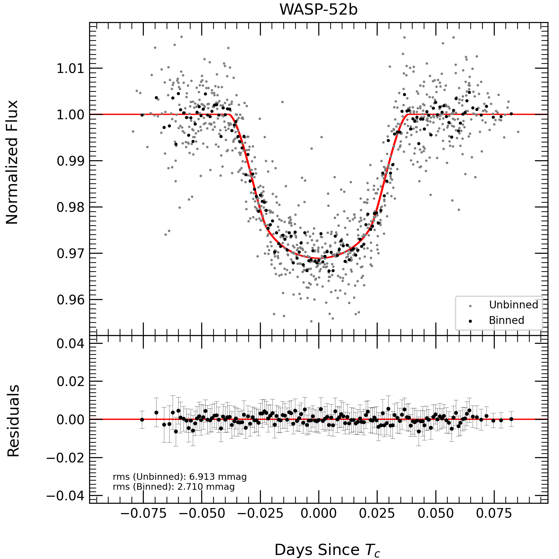
Figure 10: Fitted transit light curves of WASP-52b are shown in the top panel. Unbinned transit light curves are shown as grey points. Binned transit light curves shown as black points. Model residuals for binned transit light curves (for black points) shown in the bottom panel. The RMS of the binned data is $\sim$ 2.7 mmag and the binning is 90 s.

Based on the global fits with EXOFASTv2, the system parameters we obtained are listed in Tables 3, 4, and 5. The corresponding parameters extracted from previous studies are also listed. Our results are in good agreement with those found in the literature. Our final light curves for HATP-36b, HATP-56b and WASP-52b, along with the transit model fits, are shown in Figures 1, 5, and 8 respectively. Figures 2, 6 and 9, display the respective fits to the RV data. The global transit fits for the systems are shown in Figures 3, 7 and 10 respectively.

3.1.1 HATP-36b

Displayed in Figure 1 are our 17 transit light curves for HATP-36b along with the global best-fit models. While all the observed light curves are displayed, we only fitted those light curves (a total of 8) that had an RMS of $\leq 6mmag$ and were complete i.e., possessed both an ingress and egress, as well as, a reasonable baseline. Of course, one wants to deploy as much of the data as one can but a cutoff is still necessary to make sure that suspect and/or highly dispersive data do not dilute the extracted information. We opted for $\leq 6mmag$ as this provided a good compromise between maximum data and quality. The resulting RMS for the binned transit lightcurve for HAT-P-36b is reasonable i.e., 2.13 mmag and the residuals are also acceptable with no evident structure (see Figure 3). The corresponding RV data (including the best-fit) for HATP-36 are shown in Figure 2.

Table 3: System Parameters for HATP-36

Parameters	Units	Bakos et al. 2012	Mancini et al. 2015	Wang et al. 2019	This Work
Stellar parameter:
$M_{*}$	Mass $($$M_{\odot}$$)$	$1.022\pm 0.049$	$1.030\pm 0.029$	$1.049_{-0.046}^{+0.048}$	$1.029\pm 0.033$
$R_{*}$	Radius $($$R_{\odot}$$)$	$1.096\pm 0.056$	$1.041\pm 0.013$	$1.108_{-0.024}^{+0.025}$	$1.064\pm 0.024$
$L_{*}$	Luminosity $($$L_{\odot}$$)$	$1.03\pm 0.15$	$...$	$1.053_{-0.046}^{+0.048}$	$0.969_{-0.073}^{+0.078}$
$\rho_{*}$	Density (cgs)	$...$	$...$	$1.089_{-0.024}^{+0.025}$	$1.205_{-0.070}^{+0.077}$
$log(g_{*})$	Surface gravity $(cgs)$	$4.37\pm 0.04$	$4.416\pm 0.010$	$4.37\pm 0.04$	$4.397{\pm 0.020}$
$T_{eff}$	Effective temperature $(K)$	$5560\pm 100$	$5620\pm 40$	$5560\pm 100$	$5553{\pm 84}$
$[Fe/H]$	Metallicity	$0.26\pm 0.10$	$0.25\pm 0.09$	$0.26\pm 0.10$	$0.24{\pm 0.09}$
Planetary Parameters:
$e$	Eccentricity	$0.063\pm 0.032$	$...$	$0.063_{-0.023}^{+0.021}$	$0.051\pm{0.025}$
$P$	Period $(days)$	$1.327347\pm 0.000003$	$1.32734683\pm 0.00000048$	$1.32734660\pm 0.00000033$	$1.32734373\pm 0.00000042$
$a$	Semimajor axis $(au)$	$0.0238\pm 0.0004$	$0.02388\pm 0.00022$	$0.02402_{-0.00035}^{+0.00036}$	$0.02388\pm{0.00026}$
$M_{p}$	Mass $(M_{J})$	$1.832\pm 0.099$	$1.852\pm 0.088$	$1.925_{-0.081}^{+0.085}$	$1.871\pm{0.058}$
$R_{p}$	Radius $(R_{J})$	$1.264\pm 0.071$	$1.304\pm 0.021$	$1.357_{-0.034}^{+0.035}$	$1.285\pm 0.03$
$\rho_{p}$	Density ($\rho_{J})$	$1.12\pm 0.19$	$...$	$0.955_{-0.054}^{+0.057}$	$1.093_{-0.075}^{+0.080}$
$\log(g_{p})$	Surface gravity $(cgs)$	$3.45\pm 0.05$	$...$	$3.413\pm 0.017$	$3.448\pm 0.022$
$T_{eq}$	Equilibrium Temperature $(K)$	$1823\pm 55$	$1788\pm 15$	$1820.2_{-6.8}^{+6.7}$	$1787\pm 32$
Primary Transit Parameters:
$R_{P}/R_{*}$	Radius of planet in stellar radii	$0.1186\pm 0.0012$	$...$	$0.1260\pm 0.0011$	$0.1242\pm 0.0015$
$a/R_{*}$	Semi-major axis in stellar radii	$4.66\pm 0.22$	$...$	${4.665}_{-0.034}^{+0.035}$	${4.826}_{-0.096}^{+0.100}$
$u_{1}$ $(R$ $band)$	linear limb-darkening coeff	$...$	$...$	$0.424$	${0.420}{\pm 0.010}$
$u_{2}$ $(R$ $band)$	quadratic limb-darkening coeff	$...$	$...$	$0.250$	${0.260}\pm 0.010$
$i$	Inclination $(degrees)$	$86.0\pm 1.3$	$85.86\pm 0.21$	${85.19}_{-0.55}^{+0.72}$	$85.60\pm{0.10}$
$b$	Impact parameter	${0.312}_{-0.105}^{+0.078}$	$...$	${0.373}_{-0.062}^{+0.048}$	${0.327}\pm{0.016}$
$T_{0}$	BJD	$2455565.18144\pm{0.00020}$	$2455565.18165\pm{0.00037}$	$2456698.735910\pm{0.000149}$	$2457402.229738\pm{0.000130}$

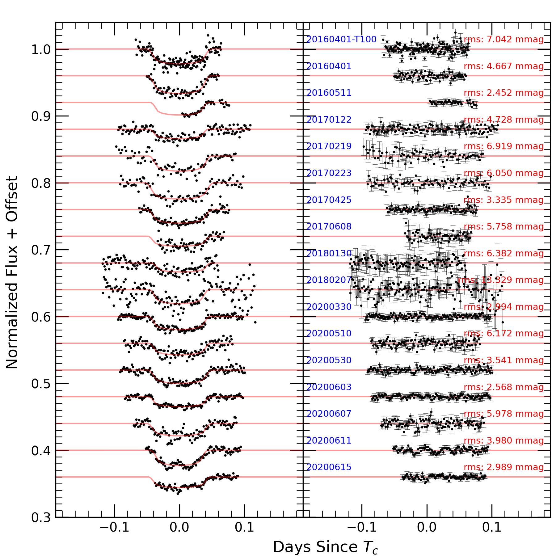
Figure 1: The left panel shows seventeen new transit light curves of HATP-36b along with the transit model fits indicated as red lines. The y-scale is arbitrarily adjusted to provide visual clarity. The right panel displays the residuals along with the dates (in the format: yyyymmdd) and the RMS (in mmag) for each light curve. With the exception of the first lightcurve, which was taken by the TUG facility, the remaining lightcurves were acquired with the ADYU facility.

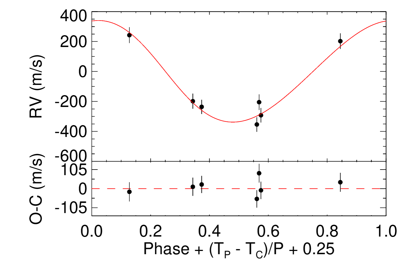
Figure 2: Distribution of the radial velocities (RVs) for HATP-36 in the top panel and the residuals in the bottom panel (Bakos et al., 2012).

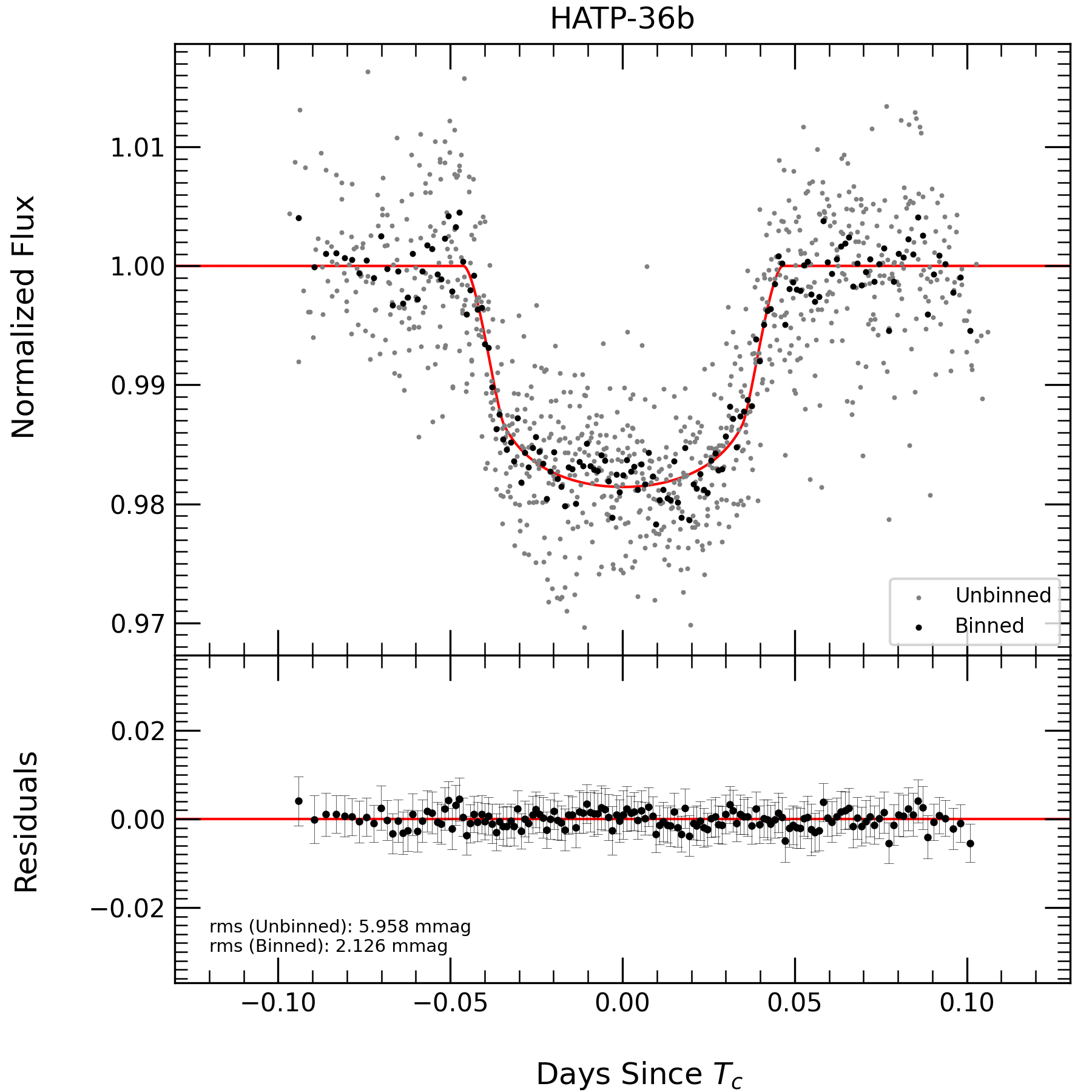
Figure 3: The fitted transit light curves of HATP-36b are shown in the top panel. Unbinned transit light curves are shown as grey points. Binned transit light curves shown as black points. Model residuals for the binned transit light curves (black points) are shown in the bottom panel. The RMS of the binned data is $\sim$ 2.1 mmag and the binning is 109 s.

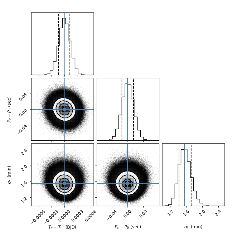
Figure 4: A corner plot showing 1-D and 2-D posterior probability distributions for the parameters of the linear ephemeris for HATP-36b.

Table 4: System Parameters for HATP-56

parameters	Units	Huang et al. 2015	This work
Stellar parameter:
$M_{*}$	Mass $($$M_{\odot}$$)$	$1.296\pm 0.036$	$1.315\pm 0.029$
$R_{*}$	Radius $($$R_{\odot}$$)$	$1.428\pm 0.030$	$1.430\pm 0.019$
$L_{*}$	Luminosity $($$L_{\odot}$$)$	$3.390\pm 0.19$	$3.420\pm{0.14}$
$\rho_{*}$	Density (cgs)	$0.627\pm 0.033$	$0.633\pm{0.025}$
$log(g_{*})$	Surface gravity $(cgs)$	$4.240\pm 0.015$	$4.246\pm 0.012$
$T_{eff}$	Effective temperature $(K)$	$6566\pm 50$	$6563\pm{49}$
$[Fe/H]$	Metallicity	$-0.077\pm 0.080$	$-0.068{\pm 0.078}$
Planetary Parameters:
$e$	Eccentricity	$<0.246$	$0.028^{+0.042}_{-0.020}$
$P$	Period $(days)$	$2.7908327\pm 0.0000047$	$2.7908278\pm{0.0000019}$
$a$	Semimajor axis $(au)$	$0.04230\pm 0.00039$	$0.04252\pm 0.00031$
$M_{p}$	Mass $(M_{J})$	$2.18\pm 0.25$	$2.11{\pm 0.21}$
$R_{p}$	Radius $(R_{J})$	$1.466\pm 0.040$	$1.387\pm 0.029$
$\rho_{p}$	Density ($\rho_{J})$	$0.86\pm 0.12$	$0.98{\pm 0.12}$
$\log(g_{p})$	Surface gravity	$3.402\pm 0.055$	$3.435{\pm 0.047}$
$T_{eq}$	Equilibrium Temperature $(K)$	$1840\pm 21$	$1835\pm 18$
Primary Transit Parameters:
$R_{P}/R_{*}$	Radius of planet in stellar radii	$0.10540\pm 0.00086$	$0.0997\pm 0.0019$
$a/R_{*}$	Semi-major axis in stellar radii	$6.37\pm 0.11$	$6.391{\pm 0.084}$
$u_{1}$ $(R$ $band)$	linear limb-darkening coeff	$...$	$0.319{\pm 0.049}$
$u_{2}$ $(R$ $band)$	quadratic limb-darkening coeff	$...$	$0.371{\pm 0.049}$
$i$	Inclination $(degrees)$	$82.13\pm 0.18$	$82.02\pm 0.15$
$b$	Impact parameter	$0.8725^{+0.0044}_{-0.0060}$	$0.8806{\pm 0.0055}$
$T_{0}$	BJD	$2456553.61645\pm 0.00042$	$2457731.345459\pm 0.000775$

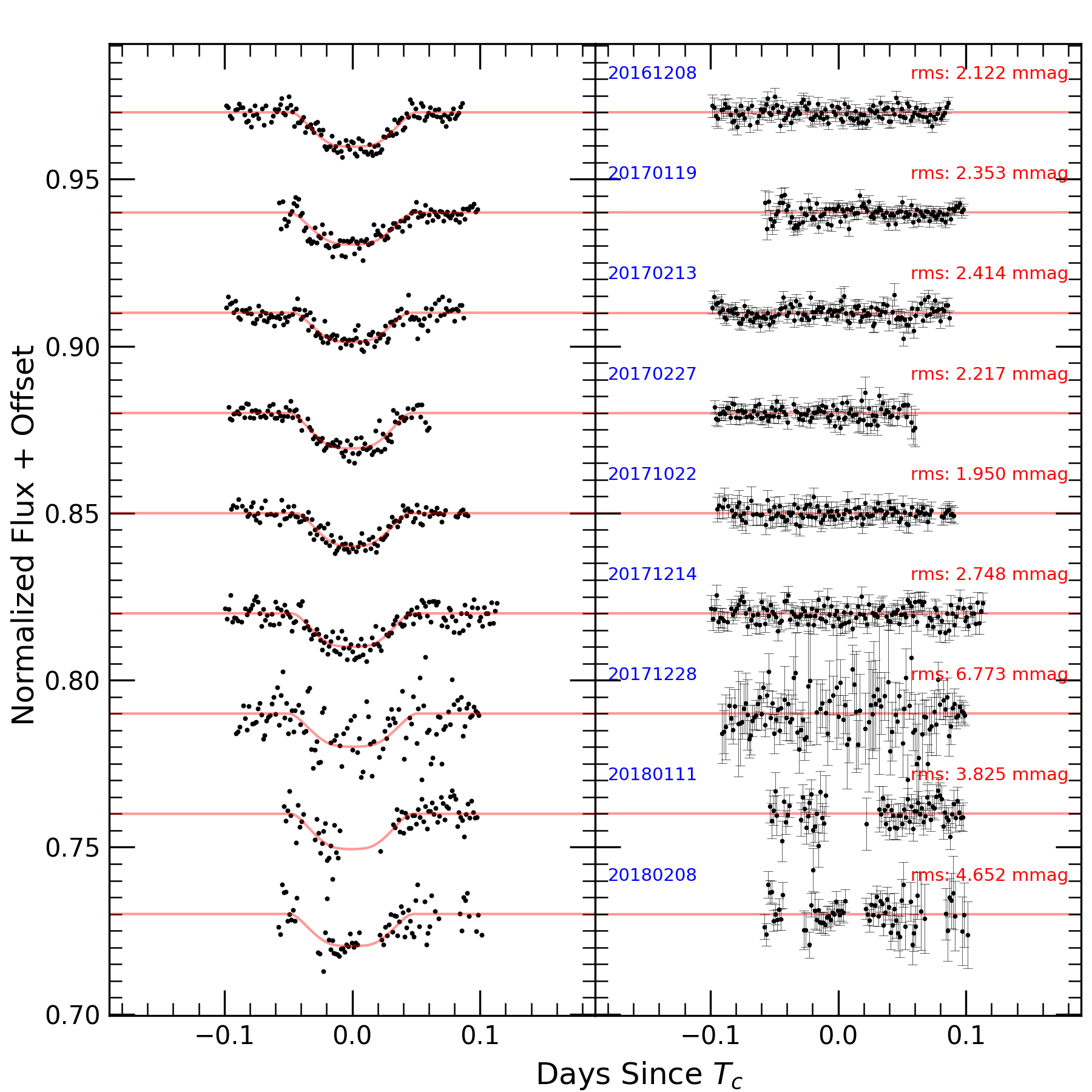
Figure 5: Nine new transit light curves of HATP-56b: All acquired with the ADYU facility. Other description is the same as in Figure 1.

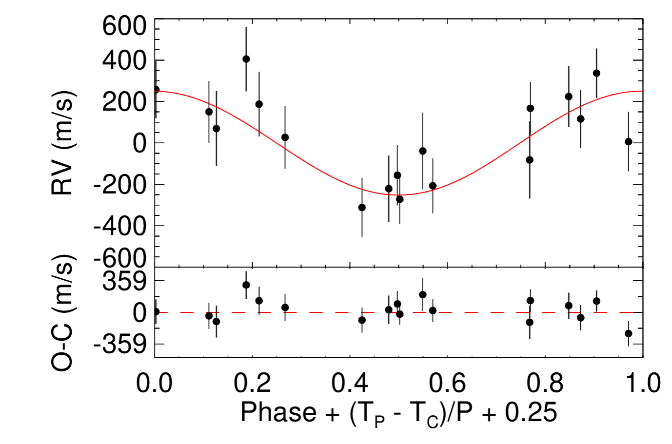
Figure 6: Distribution of radial velocities (RVs) of HATP-56 in the top panel and the residuals in the bottom panel (Huang et al., 2015).

Table 5: System Parameters for WASP-52

parameters	Units	Hebrard et al 2013	Mancini et al. 2017	This work
Stellar parameter:
$M_{*}$	Mass $($$M_{\odot}$$)$	$0.87\pm 0.03$	${0.804\pm 0.050}$	$0.857\pm 0.020$
$R_{*}$	Radius $($$R_{\odot}$$)$	$0.79\pm 0.02$	${0.786\pm 0.016}$	$0.791\pm 0.008$
$L_{*}$	Luminosity $($$L_{\odot}$$)$	$...$	$...$	${0.363}{\pm 0.025}$
$\rho_{*}$	Density $($$\rho_{\odot}$$)$	$1.76\pm 0.08$	$1.65\pm 0.02$	${1.73}{\pm 0.06}$
$log(g_{*})$	Surface gravity $(cgs)$	$4.582\pm 0.014$	${4.553\pm 0.010}$	${4.575}{\pm 0.008}$
$T_{eff}$	Effective temperature $(K)$	$5000\pm 100$	$...$	$5035\pm 82$
$[Fe/H]$	Metallicity	$0.03\pm 0.12$	$...$	$0.08\pm 0.11$
Planetary Parameters:
$e$	Eccentricity	${0(fixed)}$	$...$	${0.026}_{-0.016}^{+0.019}$
$P$	Period $(days)$	$1.7497798\pm 0.0000012$	$1.74978119\pm 0.00000052$	${1.74978111}{\pm 0.00000093}$
$a$	Semimajor axis $(au)$	$0.0272\pm 0.0003$	${0.02643\pm 0.00055}$	${0.027\pm 0.001}$
$M_{p}$	Mass $(M_{J})$	$0.46\pm 0.02$	${0.434\pm 0.024}$	${0.443\pm 0.012}$
$R_{p}$	Radius $(R_{J})$	$1.27\pm 0.03$	${1.253\pm 0.027}$	${1.281\pm 0.011}$
$\rho_{p}$	Density ($\rho_{J})$	$0.22\pm 0.02$	${0.2061\pm 0.0091}$	${0.2614}{\pm 0.0083}$
$\log(g_{p})$	Surface gravity $(cgs)$	$2.81\pm 0.03$	$...$	${2.83\pm 0.01}$
$T_{eq}$	Equilibrium Temperature $(K)$	$1315\pm 35$	$1315\pm 26$	${1314}{\pm 22}$
Primary Transit Parameters:
$R_{P}/R_{*}$	Radius of planet in stellar radii	$0.1646\pm 0.0012$	$0.16378\pm 0.0005$	${0.1665}{\pm 0.0014}$
$a/R_{*}$	Semi-major axis in stellar radii	$7.38\pm 0.02$	$...$	${7.34}{\pm 0.06}$
$u_{1}$ $(R$ $band)$	linear limb-darkening coeff.	$...$	$...$	${0.539\pm 0.034}$
$u_{2}$ $(R$ $band)$	quadratic limb-darkening coeff	$...$	$...$	${0.192\pm 0.035}$
$i$	Inclination $(degrees)$	$85.35\pm 0.20$	$85.15\pm 0.06$	${85.35\pm 0.01}$
$b$	Impact parameter	$0.60\pm 0.02$	$...$	${0.59}{\pm 0.01}$
$T_{0}$	BJD	$2455793.682175\pm 0.00009$	$2456862.79776\pm 0.00016$	$2457669.447361\pm 0.000210$

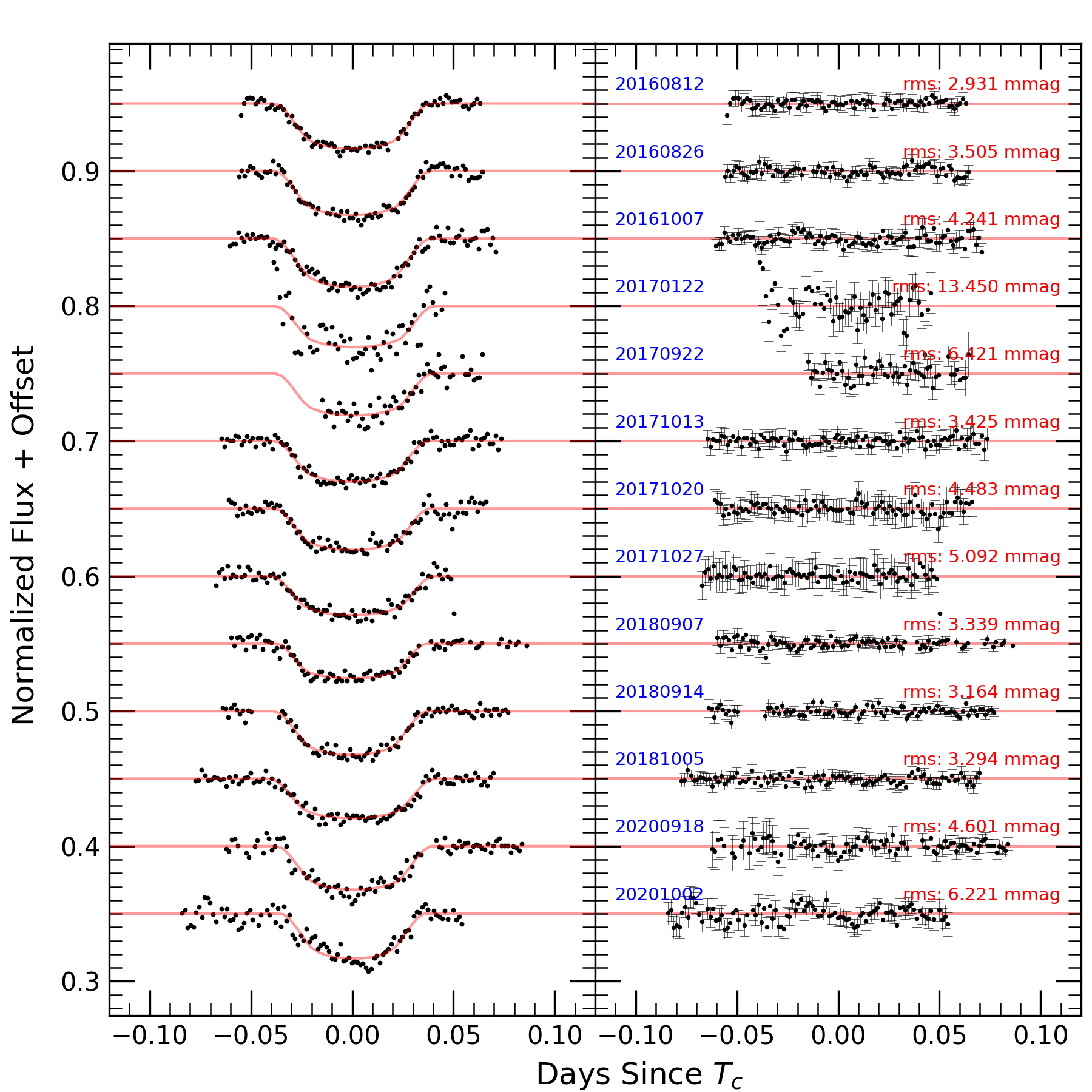
Figure 8: Thirteen new transit light curves of WASP-52b: All acquired with the ADYU facility. The other description is the same as in Figure 1.

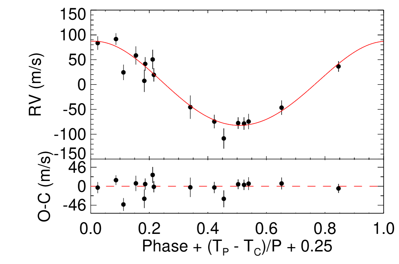
Figure 9: Distribution of radial velocities (RVs) of WASP-52 in the top panel and the residuals in the bottom panel (Hebrard et al., 2013).

To perform the TTV analysis for HATP-36b, precise mid-transit times were determined from each transit light curve, which was separately modeled by EXOFASTv2. The mid-transit time obtained for each light curve, as well as ephemeris times collected from the literature (Bakos et al., 2012; Mancini et al., 2015; Chakrabarty & Sengupta, 2019; Wang et al., 2019) are listed in Table 6. In addition, we also collected mid-transit times from the Exoplanet Transit Database (ETD) (Poddaný, Brát, & Pejcha, 2010). In the ETD, the observational data are rated by a quality index in the range 1 - 5, where the quality increases with decreasing index. Thus, we only chose the data indicated by indices 1 or 2. We converted the mid-transit times of ETD in units of Heliocentric Julian Date (HJD) to BJD through the web-gui tool (Eastman, Siverd, & Gaudi, 2010). We also note that the ETD data contain observations with different filters (I, V, and R) indicated in the figures as colored points and are included in our TTV calculations. All 88 published mid-transit data cover the time span 2010 - 2020.

We fitted the extracted mid-transit times, together with those taken from the literature, with a linear function of the form;

$$T_{C}=T_{0}+P_{orb}\times L$$ (3)

Here, the mid transit time when epoch is equal to zero $L=0$ is $T_{0}={2457402.229738}{\pm 0.000130}$ [BJD_TDB], and the orbital period is $P_{orb}={1.32734733}{\pm 0.00000017}$ days and $\sigma_{f}$ = 1.56${}_{-0.14}^{+0.16}$ mins. For completeness, 1-D and 2-D posterior probability distributions for the parameters of the updated linear ephemeris are shown as a corner plot in Figure 4.

From all mid-times, the observed - calculated (O-C) mid transit times were determined, and the O-C diagram was constructed; the plot is shown in Figure 11. Our results are shown in the upper panel (RMS $\sim 2.6min$); the lower panel displays our results overlaid with O-C data taken from the literature along with dashed lines indicating the $\pm$3$\sigma$ confidence levels. With the possible exception of three potential outliers, the majority of the points (from this work) are consistent within the 3$\sigma$ limit. As noted in the introduction, our prime motivation for monitoring HATP-36b was to follow-up on the possibility of observing stellar activity related to the surface of the host star as suggested by the work of Mancini et al. (2015). Our combined results, based on the analysis of 17 new light curves spanning a time period of approximately four years, suggest the absence of such stellar activity. However, we do note that the dispersion in our data is relatively large so it is possible the effect is masked. Moreover, as is likely, the stellar activity, if it exists (and assuming it to be similar to that observed on the surface of the Sun (Bai (2003) and references therein)), it presumably has a finite lifetime over which it persists with significant magnitude and is negligible at other times thus suggesting another possibility for its absence in our data. In principle, this second scenario is testable with an extended observation campaign.

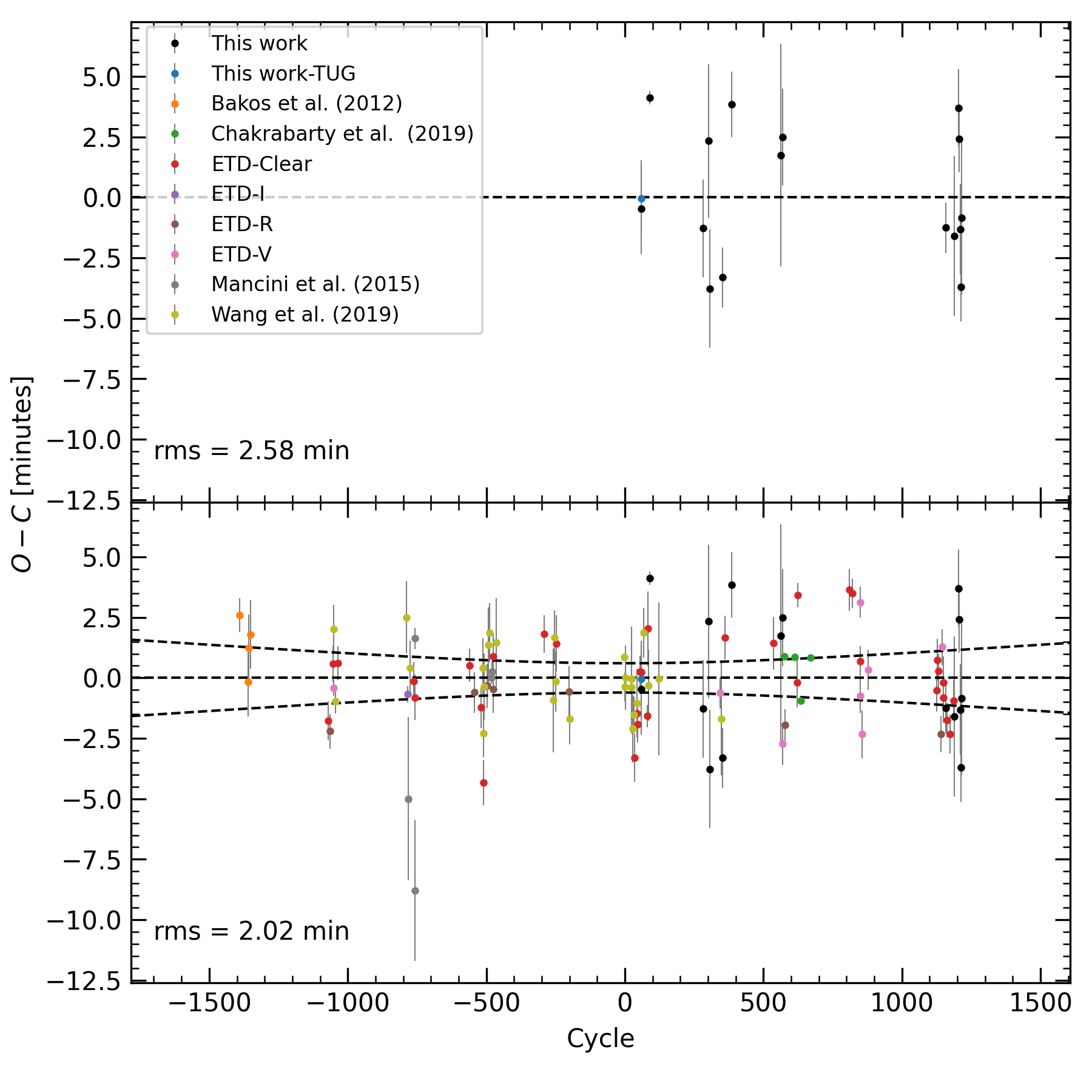
Figure 11: TTVs for HATP-36b. Our results (upper panel: black and blue points). Our results plus data taken from the literature (lower panel: colored points). Dashed (curved) lines indicate the $\pm$3$\sigma$ confidence levels. The RMS values for the data sets are $\sim$ 2.6 min and $\sim$ 2.0 min respectively.

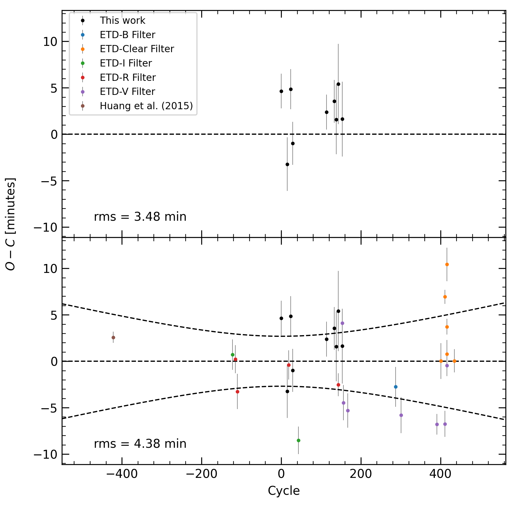
Figure 12: TTVs for HATP-56b. The description is the same as in Figure 11 The RMS values for the data sets are $\sim$ 3.5 min and $\sim$ 4.4 min respectively.

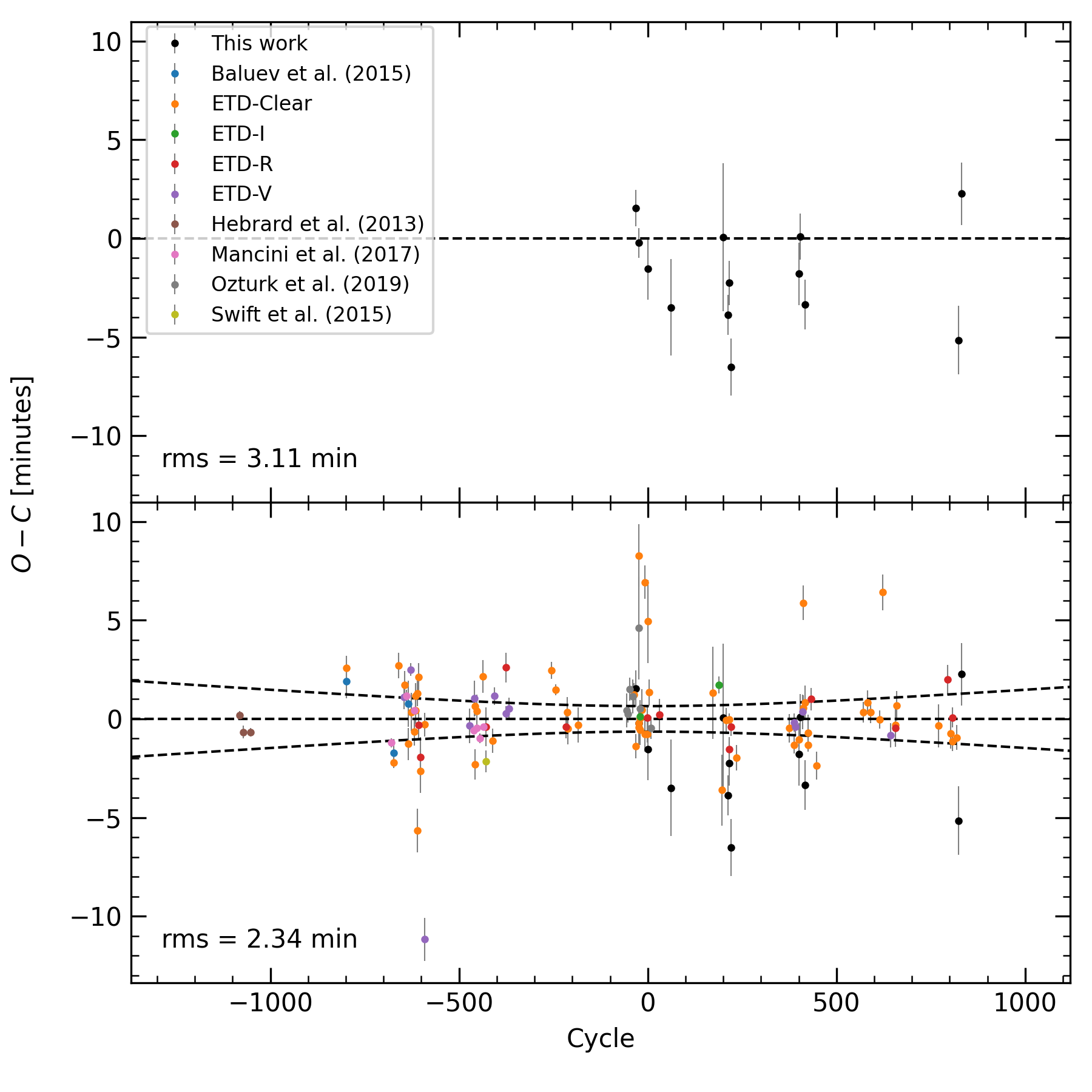
Figure 13: TTVs for WASP-52b. The description is the same as in Figure 11. The RMS values for the data sets are $\sim$ 3.1 min and $\sim$ 2.3 min respectively.

3.1.2 HATP-56b

In Figures 5 and 6, we display the 9 transit light curves of HATP-56b (although we fitted only a total of 6 of these with an RMS $\leq 3mmag$) along with global fits and the RV data, respectively. We found only 22 published mid-transit times covering the time period between 2016-2020. Our additional 9 light curves, obtained in the period 2016-2018, has significantly increased the observations for this system. Our observations and the mid-transit times collected from the literature (Poddaný, Brát, & Pejcha (2010), Huang et al. (2015)) are listed in Table 8. From the ETD data, we chose the data labeled with indices 1, 2 and 3. As stellar activity has been reported for this system, we opted to include as many reasonable data points as possible, including light curves with indices = 3, so that we could assess the robustness of the claims of intrinsic variability.

From our best-fits to the mid-transit times we obtained updated $T_{0}$, $P_{orb}$, and $\sigma_{f}$ as: $T_{0}={2457731.345473}{\pm 0.000781}$ [BJD_TDB], $P_{orb}={2.79083132}{\pm 0.00000285}$ and $\sigma_{f}$ = 4.42${}_{-0.63}^{+0.79}$ mins respectively. Using this information, we constructed the O-C diagram that is shown in Figure 12. Our results are shown by themselves in the upper panel (RMS $\sim 3.5min$); the lower panel of the figure shows our results (black points) overlaid with additional data taken from the literature (colored points) along with dashed lines indicating the $\pm$3$\sigma$ confidence levels. The majority of the data points are consistent within the 3$\sigma$ limit although, once again, there appears to be at least one point (from this work) as a possible outlier. The 1-D and 2-D posterior probability distributions for the parameters of the updated linear ephemeris are shown in Figure 14.

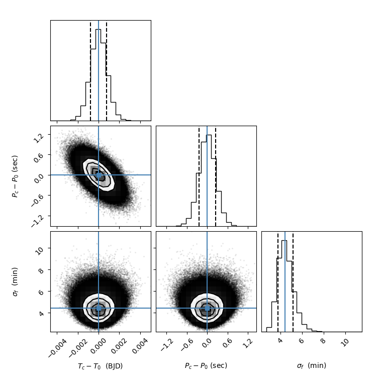
Figure 14: A corner plot showing 1-D and 2-D posterior probability distributions for the parameters of the linear ephemeris for HATP-56b.

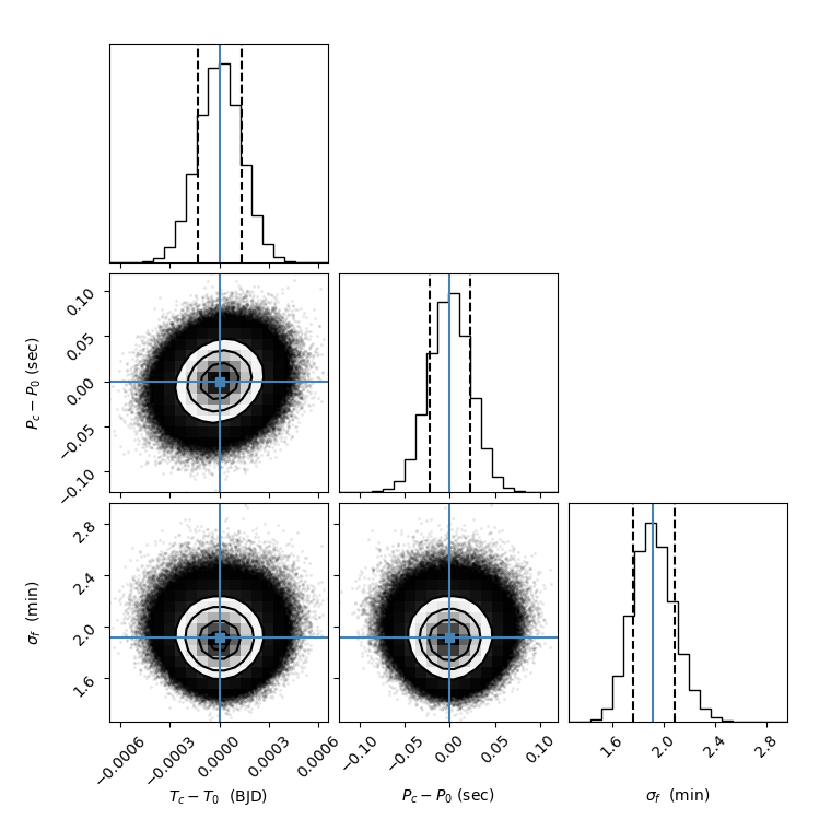
Figure 15: A corner plot showing 1-D and 2-D posterior probability distributions for the parameters of the linear ephemeris for WASP-52b.

3.1.3 WASP-52b

The 13 newly observed transits along with the global best-fits for WASP-52b and the corresponding RV data are plotted in Figures 8 and 9, respectively. Out of the 13 light curves only 10, with an RMS $\leq 6mmag$, were included in the global fit. The published data were taken from 5 different studies (Hebrard et al., 2013; Baluev et al., 2015; Swift et al., 2015; Mancini et al., 2017; Ozturk & Erdem, 2019) and ETD. We chose the data labeled with indices 1 and 2. The mid-transit times for WASP-52b are listed in Table 9. Majority of the published light curves are for the period 2010-2016. Our light curves cover the time span between 2016 to 2020, thus extending the overall time span to a total of 10 years. From the best-fitting models for each of our light curves, the mid-transit times were obtained. By fitting a linear function, the initial transit ephemeris, the orbital period and $\sigma_{f}$ were updated as follows: $T_{0}={2457669.447361}{\pm 0.000210}$ [BJD_TDB], $P_{orb}={1.74978145}{\pm 0.00000042}$ days, and $\sigma_{f}$ = 1.92${}_{-0.15}^{+0.17}$ respectively. The (O-C) values are given in Table 9, and the corresponding O-C diagram is shown in Figure 13. The upper panel of the figure displays our results (RMS $\sim 3.1min$) by themselves whereas the lower panel shows the combined data (our results, black points, plus those taken from the literature as colored points) along with curved dashed lines indicating the $\pm$3$\sigma$ confidence levels. The majority of the data points are consistent within the 3$\sigma$ limit although, once again, there appear to be possible outliers (five points from this work). The 1-D and 2-D posterior probability distributions for the parameters of the updated linear ephemeris are shown in Figure 15.

As a sanity check, we constructed Lomb-Scargle periodograms (Lomb, 1976; Scargle, 1982) for the three systems under investigation (see Figures 16, 17, and 18). The periodograms provide a measure of the distribution of power in the TTVs. The calculation is based on the O-C values and the corresponding epochs. The theoretical values of the false alarm probabilities (FAPs) of 1$\%$ and 10$\%$ are shown as dashed lines. No significant power is seen for HATP-56b and WASP-52b in the observed cycle range thus supporting the absence of structures in the respective O-C diagrams at the 3$\sigma$ level. We do note the presence of a relatively weak structure in HATP-36b ($\sim$ cycle 12.4 in Figure 18). Given the dispersion in the O-C diagram and a FAP of $\sim$10$\%$, the significance of this low-power structure is not clear.

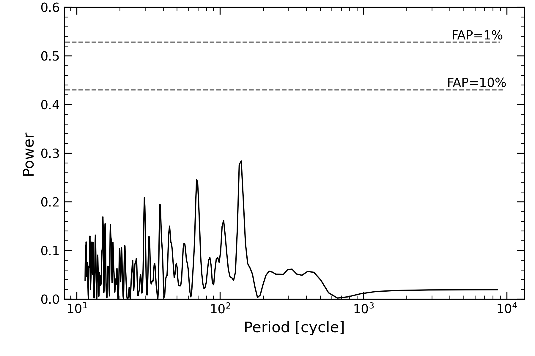
Figure 16: The Lomb-Scargle periodogram for the TTVs of HATP-56b. The false alarm probability (FAP) levels of 1$\%$ and 10$\%$ are shown as dotted horizontal lines. No significant power is detected in the observed cycle range.

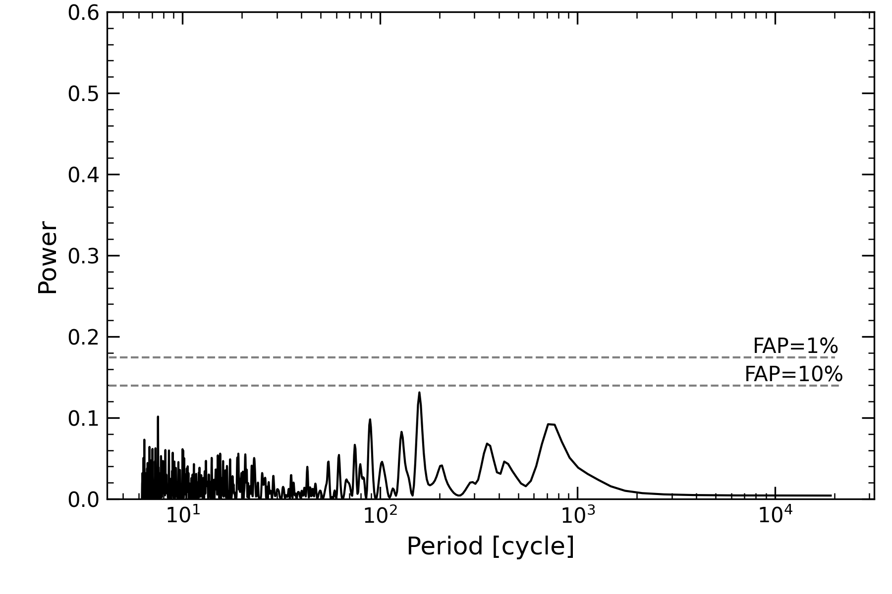
Figure 17: The Lomb-Scargle periodogram for the TTVs of WASP-52b. The other description is the same as in Figure 16.

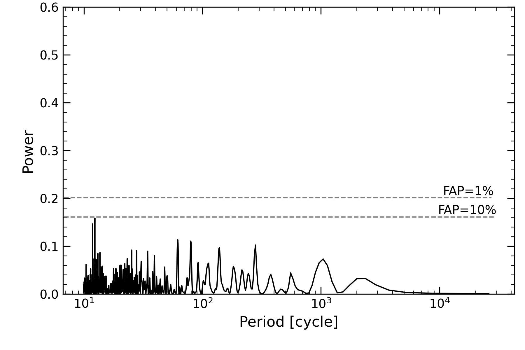
Figure 18: The Lomb-Scargle periodogram for the TTVs of HATP-36b. A narrow, relatively weak low-power structure at $\sim$ cycle 12.4 with FAP levels of $\sim$ 10$\%$ is noticeable.

4 Summary and Conclusions

We have performed long-term observations of HATP-36b, HATP-56b and WASP-52b using the 0.6 m and 1.0 m telescope facilities at Adiyaman University and TUBITAK National Observatory respectively. We have measured 17 new transit light curves for HATP-36b, 9 new transit light curves for HATP-56b, and 13 new transit light curves for WASP-52b. Using these observations in concert with published data, we have determined an updated linear ephemeris for each system. In addition, we have used these data to search for the existence of additional bodies in these systems by extracting the TTVs. O-C diagrams are constructed for each system. We summarize our main findings as follows:

• The newly extracted planetary system parameters are in very good agreement with those found in previous studies.
  

• We have determined a new ephemeris for each system. Based on the extracted periods and mid-transit times, we note that for all of the systems under study, our values agree with the respective published results within 1-2$\sigma$.
  

• An earlier study reported stellar activity on the surface of the host star in the HATP-36 system; we find no evidence of similar activity in the newly acquired 17 transit light curves spanning a time period of approximately 4 years. Indeed, we find no convincing evidence for stellar activity in the three hot-Jupiters we studied. It is possible the effect is masked in our data because of the significant dispersion. It is also possible that the stellar activity was negligible in magnitude during the period of our observations. The o-c diagrams do indicate variation at the 3$\sigma$ confidence level for a number of data points for each of the systems. However, with the level of scatter/dispersion present in the data and the irregularity of the variations it is far from clear that the potential outliers are indicative of stellar activity associated with the surface of the respective host star.
  

• We do not find strong evidence for the existence of a third (gravitationally interacting) body in any of the systems studied. The O-C diagrams indicate that the majority of the data are consistent with a linear ephemeris within the $\pm$3$\sigma$ confidence level. We do however note the presence of a number of outliers beyond the $\pm$3$\sigma$ limit for all of the systems studied. The use of data from different filters increases the likelihood of a larger dispersion in the mid-transit times because of the increased uncertainty in precisely defining the ingress and egress of the respective lightcurves.
  

Data availability

The data underlying this article are available in the article and in its online supplementary material.

Table 6: The Mid-Transit Times of HATP-36: 4-points from Bakos et al. (2012); 26-points from Wang et al. (2019), 5-points from Mancini et al. (2015), 49-points from ETD, and 4-points from Chakrabarty & Sengupta (2019)

Cycle	BJD	$(O-C)$ (d)	error	References
-1391	2455555.891400	0.001800	0.0004870	Bakos et al. (2012)a
-1360	2455597.037260	-0.000108	0.0009980	Bakos et al. (2012)a
-1357	2455601.020270	0.000860	0.0009550	Bakos et al. (2012)a
-1351	2455608.984740	0.001246	0.0009860	Bakos et al. (2012)a
-1071	2455980.639517	-0.001229	0.0005500	ETD-Clear
-1065	2455988.603296	-0.001534	0.0005000	ETD-R
-1053	2456004.533406	0.000408	0.0005200	ETD-Clear
-1051	2456007.189090	0.001397	0.0007050	Wang et al. (2019)
-1050	2456008.514756	-0.000284	0.0002400	ETD-V
-1045	2456015.151100	-0.000677	0.0003430	Wang et al. (2019)
-1035	2456028.425676	0.000426	0.0004900	ETD-Clear
-788	2456356.281780	0.001739	0.0010440	Wang et al. (2019)
-783	2456362.916308	-0.000470	0.0002400	ETD-I
-781	2456365.568000	-0.003473	0.0023400	Mancini et al. (2015)
-776	2456372.208490	0.000281	0.0007850	Wang et al. (2019)
-762	2456390.790978	-0.000094	0.0005500	ETD-Clear
-757	2456397.421700	-0.006109	0.0020200	Mancini et al. (2015)
-757	2456397.427248	-0.000561	0.0006500	ETD-Clear
-757	2456397.428940	0.001131	0.0003100	Mancini et al. (2015)
-560	2456658.915591	0.000358	0.0004800	ETD-Clear
-543	2456681.479720	-0.000417	0.0005800	ETD-R
-519	2456713.335620	-0.000853	0.0005900	ETD-Clear
-513	2456721.300850	0.000293	0.0008410	Wang et al. (2019)
-510	2456725.281000	-0.001599	0.0006760	Wang et al. (2019)
-509	2456726.606939	-0.003008	0.0006400	ETD-Clear
-507	2456729.264390	-0.000251	0.0009510	Wang et al. (2019)
-497	2456742.537889	-0.000226	0.0006400	ETD-R
-492	2456749.175800	0.000949	0.0010800	Wang et al. (2019)
-489	2456753.158190	0.001297	0.0008460	Wang et al. (2019)
-482	2456762.448340	0.000015	0.0001800	Mancini et al. (2015)
-479	2456766.430550	0.000183	0.0002800	Mancini et al. (2015)
-476	2456770.412089	-0.000320	0.0006800	ETD-R
-476	2456770.413029	0.000620	0.0006500	ETD-Clear
-465	2456785.014250	0.001021	0.0012750	Wang et al. (2019)
-292	2457014.645585	0.001267	0.0005400	ETD-Clear
-259	2457058.446140	-0.000640	0.0014890	Wang et al. (2019)
-253	2457066.412020	0.001156	0.0007760	Wang et al. (2019)
-250	2457070.392800	-0.000106	0.0008580	Wang et al. (2019)
-247	2457074.375934	0.000986	0.0008100	ETD-Clear
-201	2457135.432534	-0.000391	0.0007300	ETD-R
-199	2457138.086450	-0.001169	0.0007330	Wang et al. (2019)
-3	2457398.248300	0.000604	0.0000880	Wang et al. (2019)
0	2457402.229480	-0.000258	0.0004120	Wang et al. (2019)
3	2457406.211790	0.000010	0.0009220	Wang et al. (2019)
24	2457434.085800	-0.000274	0.0013190	Wang et al. (2019)
25	2457435.413400	-0.000022	0.0014930	Wang et al. (2019)
28	2457439.394010	-0.001454	0.0009780	Wang et al. (2019)
34	2457447.358490	-0.001058	0.0005280	Wang et al. (2019)
35	2457448.684605	-0.002290	0.0007000	ETD-Clear
43	2457459.304940	-0.000734	0.0009830	Wang et al. (2019)
44	2457460.632005	-0.001016	0.0006700	ETD-Clear
46	2457463.286385	-0.001331	0.0005200	ETD-Clear
54	2457473.906675	0.000181	0.0004500	ETD-Clear
59	2457480.542900	-0.000331	0.0013000	This work
59	2457480.543200	-0.000031	0.0011000	This work-TUG
59	2457480.543396	0.000165	0.0006400	ETD-Clear
67	2457491.163310	0.001300	0.0007150	Wang et al. (2019)
80	2457508.416426	-0.001099	0.0003200	ETD-Clear
83	2457512.400976	0.001409	0.0010700	ETD-Clear
85	2457515.054050	-0.000212	0.0010210	Wang et al. (2019)
89	2457520.366510	0.002859	0.0001900	This work

Table 7: continued

The Mid-Transit Times of HATP-36 Cycle BJD $(O-C)$ (d) error References 122 2457564.166080 -0.000033 0.0021960 Wang et al. (2019) 282 2457776.540800 -0.000886 0.0014000 This work 303 2457804.417600 0.001620 0.0022000 This work 306 2457808.395400 -0.002622 0.0017000 This work 344 2457858.836783 -0.000437 0.0004500 ETD-V 348 2457864.145440 -0.001170 0.0016290 Wang et al. (2019) 352 2457869.453700 -0.002299 0.0008600 This work 361 2457881.403284 0.001159 0.0006300 ETD-Clear 385 2457913.261140 0.002679 0.0009400 This work 536 2458113.688899 0.000991 0.0007500 ETD-Clear 563 2458149.527500 0.001214 0.0032000 This work 569 2458157.488471 -0.001899 0.0006100 ETD-V 569 2458157.492100 0.001730 0.0014000 This work 575 2458165.455070 0.000616 0.0000070 Chakrabarty & Sengupta (2019) 578 2458169.435141 -0.001355 0.0004500 ETD-R 614 2458217.221600 0.000600 0.0000080 Chakrabarty & Sengupta (2019) 621 2458226.512303 -0.000128 0.0007100 ETD-Clear 624 2458230.496853 0.002380 0.0003500 ETD-Clear 635 2458245.094640 -0.000654 0.0000070 Chakrabarty & Sengupta (2019) 669 2458290.225690 0.000587 0.0000070 Chakrabarty & Sengupta (2019) 811 2458478.710952 0.002528 0.0006000 ETD-Clear 820 2458490.656972 0.002422 0.0004200 ETD-Clear 850 2458530.474453 -0.000517 0.0004900 ETD-V 850 2458530.475453 0.000483 0.0004300 ETD-Clear 850 2458530.477143 0.002173 0.0004400 ETD-V 856 2458538.437434 -0.001620 0.0006900 ETD-V 878 2458567.640925 0.000230 0.0005700 ETD-V 1125 2458895.495126 -0.000360 0.0006100 ETD-Clear 1128 2458899.478046 0.000518 0.0006000 ETD-Clear 1131 2458903.459776 0.000206 0.0004800 ETD-Clear 1140 2458915.404086 -0.001610 0.0005200 ETD-R 1146 2458923.370667 0.000887 0.0005200 ETD-V 1149 2458927.351257 -0.000565 0.0007200 ETD-Clear 1149 2458927.351687 -0.000135 0.0007600 ETD-Clear 1158 2458939.297080 -0.000868 0.0007200 This work 1162 2458944.606127 -0.001210 0.0004900 ETD-Clear 1174 2458960.533898 -0.001607 0.0005600 ETD-Clear 1186 2458976.463018 -0.000655 0.0006000 ETD-Clear 1189 2458980.444600 -0.001115 0.0023000 This work 1204 2459000.358500 0.002575 0.0011000 This work 1207 2459004.339640 0.001673 0.0009500 This work 1210 2459008.319100 -0.000909 0.0013000 This work 1213 2459012.299480 -0.002571 0.0009900 This work 1216 2459016.283500 -0.000593 0.0022000 This work ^a Mid-transit times calculated by Wang et al. (2019) from observations of Bakos et al. (2012)

Table 8: The Mid-Transit Times of HATP-56: 20-points from ETD and 1-point from Huang et al. (2015)

Cycle	BJD	$(O-C)$ (d)	error	References
-422	2456553.616450	0.001827	0.00042	Huang et al. (2015)
-122	2457390.864544	0.000512	0.00114	ETD-I
-115	2457410.400025	0.000173	0.00105	ETD-R
-110	2457424.351766	-0.002243	0.00132	ETD-R
0	2457731.348700	0.003227	0.00130	This work
15	2457773.205700	-0.002243	0.00200	This work
19	2457784.370992	-0.000263	0.00109	ETD-R
24	2457798.328800	0.003375	0.00150	This work
29	2457812.278900	-0.000681	0.00160	This work
43	2457851.345304	-0.005904	0.00103	ETD-I
114	2458049.501900	0.001657	0.00130	This work
133	2458102.528500	0.002462	0.00160	This work
138	2458116.481300	0.001105	0.00260	This work
143	2458130.432595	-0.001749	0.00086	ETD-R
143	2458130.438100	0.003749	0.00300	This work
153	2458158.343800	0.001135	0.00280	This work
153	2458158.345516	0.002858	0.00081	ETD-V
156	2458166.712056	-0.003096	0.00132	ETD-V
167	2458197.410617	-0.003680	0.00128	ETD-V
287	2458532.312145	-0.001916	0.00148	ETD-B
301	2458571.381665	-0.004035	0.00135	ETD-V
391	2458822.555807	-0.004716	0.00077	ETD-V
401	2458850.468847	0.000011	0.00134	ETD-Clear
411	2458878.372457	-0.004693	0.00098	ETD-V
411	2458878.381967	0.004817	0.00053	ETD-Clear
416	2458892.330987	-0.000320	0.0008	ETD-V
416	2458892.331847	0.000540	0.00104	ETD-Clear
416	2458892.333887	0.002580	0.00059	ETD-Clear
416	2458892.338547	0.007240	0.00125	ETD-Clear
435	2458945.357126	0.000023	0.00087	ETD-Clear

Table 9: The Mid-Transit Times of WASP-52: 89-points from ETD, 3-points from Hebrard et al. (2013), 3-points from Baluev et al. (2015), 7-points from Ozturk & Erdem (2019), 7-points from Mancini et al. (2017), 1-point from Swift et al. (2015)

Cycle	BJD	$(O-C)$ (d)	error	References
-1082	2455776.183950	0.000123	0.00015	Hebrard et al. (2013)a
-1072	2455793.681180	-0.000462	0.00022	Hebrard et al. (2013)a
-1052	2455828.676800	-0.000471	0.00015	Hebrard et al. (2013)a
-799	2456271.373300	0.001321	0.00059	Baluev et al. (2015)b
-799	2456271.373781	0.001802	0.00042	ETD-Clear
-680	2456479.595130	-0.000842	0.00016	Mancini et al. (2017)
-673	2456491.842899	-0.001543	0.00019	ETD-Clear
-673	2456491.843240	-0.001202	0.00026	Baluev et al. (2015)b
-660	2456514.593480	0.001879	0.00044	ETD-Clear
-645	2456540.839081	0.000758	0.00041	ETD-V
-644	2456542.589301	0.001197	0.00049	ETD-Clear
-640	2456549.588050	0.000820	0.00020	Mancini et al. (2017)
-635	2456558.335251	-0.000887	0.00057	ETD-Clear
-635	2456558.336670	0.000532	0.00082	Baluev et al. (2015)b
-628	2456570.586342	0.001734	0.00023	ETD-V
-627	2456572.334632	0.000243	0.00068	ETD-Clear
-619	2456586.332182	-0.000459	0.00049	ETD-Clear
-619	2456586.332930	0.000289	0.00012	Mancini et al. (2017)
-616	2456591.582273	0.000288	0.00047	ETD-Clear
-615	2456593.332583	0.000816	0.00044	ETD-Clear
-611	2456600.326963	-0.003929	0.00077	ETD-Clear
-611	2456600.331783	0.000891	0.00045	ETD-Clear
-608	2456605.581703	0.001466	0.00050	ETD-Clear
-607	2456607.329813	-0.000205	0.00049	ETD-R
-603	2456614.327303	-0.001841	0.00077	ETD-Clear
-603	2456614.327803	-0.001341	0.00071	ETD-R
-591	2456635.318764	-0.007758	0.00076	ETD-V
-591	2456635.326324	-0.000198	0.00042	ETD-Clear
-472	2456843.550270	-0.000245	0.00060	ETD-V
-461	2456862.797710	-0.000401	0.00006	Mancini et al. (2017)
-460	2456864.548610	0.000718	0.00063	ETD-V
-457	2456869.795640	-0.001597	0.00053	ETD-Clear
-457	2456869.797690	0.000453	0.00034	ETD-Clear
-453	2456876.796050	-0.000312	0.00011	Mancini et al. (2017)
-453	2456876.796640	0.000278	0.00057	ETD-Clear
-445	2456890.793930	-0.000684	0.00018	Mancini et al. (2017)
-437	2456904.794361	0.001495	0.00058	ETD-Clear
-436	2456906.542370	-0.000277	0.00008	Mancini et al. (2017)
-429	2456918.789620	-0.001497	0.00039	Swift et al. (2015)
-428	2456920.540622	-0.000277	0.00069	ETD-R
-411	2456950.286413	-0.000770	0.00042	ETD-Clear
-407	2456957.287113	0.000804	0.00031	ETD-V
-375	2457013.279514	0.000198	0.00025	ETD-V
-375	2457013.281124	0.001808	0.00052	ETD-R
-367	2457027.277924	0.000357	0.00038	ETD-V
-256	2457221.505008	0.001699	0.00030	ETD-Clear
-244	2457242.501708	0.001022	0.00020	ETD-Clear
-216	2457291.494279	-0.000288	0.00040	ETD-R
-213	2457296.744149	0.000237	0.00052	ETD-Clear
-212	2457298.493359	-0.000334	0.00057	ETD-Clear
-184	2457347.487359	-0.000215	0.00062	ETD-Clear
-56	2457571.459900	0.000300	0.00060	Ozturk & Erdem (2019)
-52	2457578.458900	0.000174	0.00030	Ozturk & Erdem (2019)
-48	2457585.458900	0.001048	0.00040	Ozturk & Erdem (2019)
-40	2457599.456900	0.000797	0.00060	Ozturk & Erdem (2019)
-36	2457606.456077	0.000848	0.00040	ETD-Clear
-32	2457613.453397	-0.000958	0.00042	ETD-Clear
-32	2457613.455430	0.001075	0.00064	This work
-24	2457627.452297	-0.000309	0.00063	ETD-Clear
-24	2457627.452447	-0.000159	0.00036	ETD-Clear
-24	2457627.452450	-0.000156	0.00052	This work
-24	2457627.455800	0.003194	0.00180	Ozturk & Erdem (2019)
-24	2457627.458357	0.005751	0.00110	ETD-Clear
-21	2457632.702027	0.000076	0.00021	ETD-I

Table 10: continued

The Mid-Transit Times of WASP-52 Cycle BJD $(O-C)$ (d) error References -20 2457634.451347 -0.000385 0.00053 ETD-Clear -20 2457634.451757 0.000025 0.00037 ETD-Clear -20 2457634.452100 0.000368 0.00030 Ozturk & Erdem (2019) -16 2457641.451177 0.000319 0.00073 ETD-Clear -8 2457655.448567 -0.000543 0.00062 ETD-Clear -8 2457655.453917 0.004807 0.00059 ETD-Clear -1 2457667.697047 -0.000533 0.00029 ETD-Clear -1 2457667.697617 0.000037 0.00037 ETD-R 0 2457669.446300 -0.001061 0.00110 This work 0 2457669.450787 0.003426 0.00147 ETD-Clear 4 2457676.447417 0.000930 0.00046 ETD-Clear 8 2457683.445300 -0.000313 0.00040 Ozturk & Erdem (2019) 31 2457723.690726 0.000140 0.00057 ETD-R 61 2457776.181600 -0.002430 0.00170 This work 172 2457970.410691 0.000919 0.00162 ETD-Clear 188 2457998.407460 0.001185 0.00030 ETD-I 196 2458012.402020 -0.002507 0.00125 ETD-Clear 200 2458019.403700 0.000048 0.00260 This work 207 2458031.652089 -0.000034 0.00041 ETD-Clear 212 2458040.398340 -0.002690 0.00071 This work 215 2458045.649309 -0.001065 0.00042 ETD-R 215 2458045.650359 -0.000015 0.00021 ETD-Clear 216 2458047.398590 -0.001566 0.00078 This work 220 2458054.394760 -0.004521 0.00100 This work 220 2458054.399009 -0.000272 0.00033 ETD-R 235 2458080.644628 -0.001375 0.00045 ETD-Clear 375 2458325.615078 -0.000329 0.00050 ETD-Clear 387 2458346.611867 -0.000917 0.00029 ETD-Clear 387 2458346.612657 -0.000127 0.00032 ETD-V 391 2458353.611627 -0.000283 0.00031 ETD-V 400 2458369.358700 -0.001243 0.00110 This work 400 2458369.359226 -0.000717 0.00038 ETD-Clear 404 2458376.359130 0.000061 0.00081 This work 411 2458388.607785 0.000246 0.00060 ETD-V 412 2458390.357705 0.000384 0.00044 ETD-Clear 412 2458390.361405 0.004084 0.00060 ETD-Clear 416 2458397.354120 -0.002327 0.00088 This work 416 2458397.357025 0.000578 0.00060 ETD-Clear 424 2458411.353775 -0.000923 0.00024 ETD-Clear 424 2458411.354215 -0.000483 0.00064 ETD-Clear 432 2458425.353644 0.000694 0.00039 ETD-R 447 2458451.598023 -0.001649 0.00049 ETD-Clear 571 2458668.572803 0.000231 0.00036 ETD-Clear 583 2458689.570531 0.000581 0.00041 ETD-Clear 591 2458703.568431 0.000230 0.00038 ETD-Clear 615 2458745.562929 -0.000027 0.00032 ETD-Clear 623 2458759.565659 0.004451 0.00063 ETD-Clear 644 2458796.306037 -0.000581 0.00043 ETD-V 656 2458817.303676 -0.000320 0.00066 ETD-R 656 2458817.303776 -0.000220 0.00025 ETD-Clear 660 2458824.303586 0.000464 0.00052 ETD-Clear 771 2459018.528617 -0.000246 0.00076 ETD-Clear 795 2459060.524995 0.001377 0.00053 ETD-R 803 2459074.521354 -0.000516 0.00053 ETD-Clear 807 2459081.520214 -0.000781 0.00036 ETD-Clear 807 2459081.521044 0.000049 0.00035 ETD-R 819 2459102.517714 -0.000659 0.00044 ETD-Clear 824 2459111.263700 -0.003580 0.00120 This work 832 2459125.267100 0.001568 0.00110 This work ^a Mid-transit times calculated by Mancini et al. (2017) from observations of Hebrard et al. (2013) ^b Mid-transit times calculated by Ozturk & Erdem (2019) from observations of Baluev et al. (2015)

Appendix A

Figure 19: The posterior distributions obtained for the main stellar and planetary parameters of HATP-36 system.

Figure 20: The posterior distributions obtained for the main stellar and planetary parameters of HATP-56 system.

Figure 21: The posterior distributions obtained for the main stellar and planetary parameters of WASP-52 system.

References

- Agol et al. (2005) Agol E., Steffen J., Sari R., Clarkson W., 2005, MNRAS, 359, 567
- Bai (2003) Bai, T., 2003, ApJ, 591, 406
- Bakos et al. (2004) Bakos G. Á., Noyes, R. W., Kovács, G., et al. 2004, PASP, 116, 266
- Bakos et al. (2012) Bakos G. Á., Hartman J. D., Torres G., Béky B., Latham D. W., Buchhave L. A., Csubry Z., et al., 2012, AJ, 144, 19
- Baluev et al. (2015) Baluev R. V., Sokov E. N., Shaidulin V. S., Sokova I. A., Jones H. R. A., Tuomi M., Anglada-Escudé G., et al., 2015, MNRAS, 450, 3101. doi:10.1093/mnras/stv788
- Barros et al. (2013) Barros, S. C. C.; Boue, G.; Gibson, N. P.; Pollacco, D. L.; Santerne, A. et al. 2013, MNRAS, 430, 3032
- Boue et al. (2012) Bouee, G., Oshagh, M., Montalto, M., & Santos, N. C. 2012, MNRAS, 422, L57
- Bruno et al. (2018) Bruno, Giovanni; Lewis, Nikole K.; Stevenson, Kevin B.; Filippazzo, Joseph; Hill, Matthew et al., 2018, AJ, 156, 124
- Chakrabarty & Sengupta (2019) Chakrabarty A., Sengupta S., 2019, AJ, 158, 39
- Chen et al. (2017) Chen, G.; Pallé, E.; Nortmann, L.; Murgas, F.; Parviainen, H.; Nowak, G., 2017, A&A, 600, 11
- Collins et al. (2017) Collins K. A., Kielkopf J. F., Stassun K. G., 2017, AJ, 153, 78
- Eastman (2017) Eastman, J. 2017, EXOFASTv2: Generalized publication-quality exoplanet
- Eastman et al. (2019) Eastman, Jason D. and Rodriguez, Joseph E. and Agol, Eric and Stassun, Keivan G. and Beatty, Thomas G. and Vanderburg, Andrew and Gaudi, B. Scott and Collins, Karen A. and Luger, Rodrigo, 2019, arXiv:1907.09480
- Dotter (2016) Dotter, A. 2016, ApJS, 222, 8
- Eastman, Gaudi, & Agol (2013) Eastman J., Gaudi B. S., Agol E., 2013, PASP, 125, 83 modeling code, Astrophysics Source Code Library, ascl:1710.003
- Eastman, Siverd, & Gaudi (2010) Eastman J., Siverd R., Gaudi B. S., 2010, PASP, 122, 935. doi:10.1086/655938
- Ford (2006) Ford, E. B. 2006, ApJ, 642, 505
- Ford & Holman (2007) Ford, E. B.; Holman, M. J., 2007, ApJ, 664, 51
- Foreman-Mackey et al. (2013) Foreman-Mackey D., Hogg D. W., Lang D., Goodman J., 2013, PASP, 125, 306. doi:10.1086/670067
- Gelman & Rubin (1992) Gelman, A., & Rubin, D. B. 1992, StaSc, 7, 457
- Goodman & Weare (2010) Goodman J., Weare J., 2010, CAMCS, 5, 65.
- Goździewski et al. (2015) Goździewski K., Słowikowska A., Dimitrov D., Krzeszowski K., Żejmo M., Kanbach G., Burwitz V., et al., 2015, MNRAS, 448, 1118.
- Hebrard et al. (2013) Hebrard G., Collier Cameron A., Brown D. J. A., Díaz R. F., Faedi F., Smalley B., Anderson D. R., et al., 2013, A&A, 549, A134
- Huang et al. (2015) Huang C. X., Hartman J. D., Bakos G. Á., Penev K., Bhatti W., Bieryla A., de Val-Borro M., et al., 2015, AJ, 150, 85
- Ioannidis, Huber & Schmitt (2016) Ioannidis, P.; Huber, K. F.; Schmitt, J. H. M. M., 2016, A&A,585, 72
- Kirk et al. (2016) Kirk, J.; Wheatley, P. J.; Louden, T.; Littlefair, S. P.; Copperwheat, C. M. et al. 2016, MNRAS, 463. 2922K
- Lithwick et al. (2012) Lithwick, Y., Xie, J., & Wu, Y. 2012, ApJ, 761, 122
- Lomb (1976) Lomb, N.R., 1976, Ap&SS, 39, 447
- Louden et al. (2017) Louden, Tom; Wheatley, Peter J.; Irwin, Patrick G. J.; Kirk, James; Skillen, Ian, 2017, MNRAS, 470, 742
- Maciejewski et al. (2013) Maciejewski, G.; Puchalski, D.; Saral, G.; Derman, E.; Kitze, M. et al. 2013, IBVS, 6082, 1
- Mancini et al. (2015) Mancini L., Esposito M., Covino E., Raia G., Southworth J., Tregloan-Reed J., Biazzo K., et al., 2015, A&A, 579, A136
- Mancini et al. (2017) Mancini L., Southworth J., Raia G., Tregloan-Reed J., Molliere P., Bozza V., Bretton M., et al., 2017, MNRAS, 465, 843. doi:10.1093/mnras/stw1987
- Mayor & Queloz (1995) Mayor, M.; Queloz, D. 1995, Nature, 378, 355
- Nesvorny & Morbidelli (2008) Nesvorny, D.; Morbidelli, A., 2008, ApJ, 688, 636
- Newville et al. (2016) Newville M., Stensitzki T., Allen D. B., Rawlik M., Ingargiola A., Nelson A., 2016, ascl.soft. ascl:1606.014
- Oshagh et al. (2013) Oshagh, M.; Santos, N. C.; Boisse, I.; Boué, G.; Montalto, M. et al. 2013, A&A, 556, 19
- Ozturk & Erdem (2019) Ozturk O., Erdem A., 2019, MNRAS, 486, 2290. doi:10.1093/mnras/stz747
- Payne et al. (2010) Payne, M. J.; Ford, E. B.; Veras, D., 2010, ApJ, 712, 86
- Poddaný, Brát, & Pejcha (2010) Poddaný S., Brát L., Pejcha O., 2010, NewA, 15, 297
- Scargle (1982) Scargle, J.D., 1982, ApJ, 263, 835
- Swift et al. (2015) Swift J. J., Bottom M., Johnson J. A., Wright J. T., McCrady N., Wittenmyer R. A., Plavchan P., et al., 2015, JATIS, 1, 027002. doi:10.1117/1.JATIS.1.2.027002
- Ter Braak (2006) Ter Braak C. J. F., 2006, S&C, 16, 239
- Tregloan-Reed et al. (2013) Tregloan-Reed J., Southworth J., Tappert C., 2013, MNRAS, 428, 3671
- Tregloan-Reed et al. (2015) Tregloan-Reed J., Southworth J., Burgdorf M., Novati S. C., Dominik M., Finet F., Jørgensen U. G., et al., 2015, MNRAS, 450, 1760
- Tregloan-Reed et al. (2018) Tregloan-Reed J., Southworth J., Mancini L., Mollière P., Ciceri S., Bruni I., Ricci D., et al., 2018, MNRAS, 474, 5485
- Veras et al. (2011) Veras, D., Ford, E. B., & Payne, M. J. 2011, ApJ, 727, 74
- Wang et al. (2019) Wang Y.-H., Wang S., Hinse T. C., Wu Z.-Y., Davis A. B., Hori Y., Yoon J.-N., et al., 2019, AJ, 157, 82
- Zhou et al. (2016) Zhou, George; Latham, David W.; Bieryla, Allyson; Beatty, Thomas G.; Buchhave, Lars A. et al. 2016, MNRAS, 460, 3376