A PTAS for the horizontal rectangle stabbing problem

Abstract

We study rectangle stabbing problems in which we are given $n$ axis-aligned rectangles in the plane that we want to stab, i.e., we want to select line segments such that for each given rectangle there is a line segment that intersects two opposite edges of it. In the horizontal rectangle stabbing problem (Stabbing), the goal is to find a set of horizontal line segments of minimum total length such that all rectangles are stabbed. In general rectangle stabbing problem, also known as horizontal-vertical stabbing problem (HV-Stabbing), the goal is to find a set of rectilinear (i.e., either vertical or horizontal) line segments of minimum total length such that all rectangles are stabbed. Both variants are NP-hard. Chan, van Dijk, Fleszar, Spoerhase, and Wolff [CvDF⁺18] initiated the study of these problems by providing constant approximation algorithms. Recently, Eisenbrand, Gallato, Svensson, and Venzin [EGSV21] have presented a QPTAS and a polynomial-time 8-approximation algorithm for Stabbing but it is was open whether the problem admits a PTAS.

In this paper, we obtain a PTAS for Stabbing, settling this question. For HV-Stabbing, we obtain a $(2+\varepsilon)$-approximation. We also obtain PTASes for special cases of HV-Stabbing: (i) when all rectangles are squares, (ii) when each rectangle’s width is at most its height, and (iii) when all rectangles are $\delta$-large, i.e., have at least one edge whose length is at least $\delta$, while all edge lengths are at most 1. Our result also implies improved approximations for other problems such as generalized minimum Manhattan network.

1 Introduction

Rectangle stabbing problems are natural geometric optimization problems. Here, we are given a set of $n$ axis-parallel rectangles $\mathcal{R}$ in the two-dimensional plane. For each rectangle $R_{i}\in\mathcal{R}$, we are given points $(x_{1}^{(i)},y_{1}^{(i)}),(x_{2}^{(i)},y_{2}^{(i)})\in\mathbb{R}^{2}$ that denote its bottom-left and top-right corners, respectively. Also, we denote its width and height by $w_{i}:=x_{2}^{(i)}-x_{1}^{(i)}$ and $h_{i}:=y_{2}^{(i)}-y_{1}^{(i)}$, respectively. Our goal is to compute a set of line segments $\mathcal{L}$ that stab all input rectangles. We call a rectangle stabbed if a segment $\ell\in\mathcal{L}$ intersects both of its horizontal or both of its vertical edges. We study several variants. In the horizontal rectangle stabbing problem (Stabbing) we want to find a set of horizontal segments of minimum total length such that each rectangle is stabbed. The general rectangle stabbing (HV-Stabbing) problem generalizes Stabbing and involves finding a set of axis parallel segments of minimum total length such that each rectangle in $\mathcal{R}$ is stabbed. The general square stabbing (Square-Stabbing) problem is a special case of HV-Stabbing where all rectangles in the input instance are squares. These problems have applications in bandwidth allocation, message scheduling with time-windows on a direct path, and geometric network design [CvDF⁺18, BMSV⁺09, DFK⁺18].

Note that Stabbing and HV-Stabbing are special cases of weighted geometric set cover, where the rectangles correspond to elements and potential line segments correspond to sets, and the weight of a set equals the length of the corresponding segment. A set contains an element if the corresponding line segment stabs the corresponding rectangle. This already implies an $O(\log n)$-approximation algorithm [Chv79] for HV-Stabbing and Stabbing.

Chan, van Dijk, Fleszar, Spoerhase, and Wolff [CvDF⁺18] initiated the study of Stabbing. They proved Stabbing to be NP-hard via a reduction from planar vertex cover. Also, they presented a constant factor approximation using decomposition techniques and the quasi-uniform sampling method [Var10] for weighted geometric set cover. In particular, they showed that Stabbing instances can be decomposed into two disjoint laminar set cover instances of small shallow cell complexity for which the quasi-uniform sampling yields a constant approximation using techniques from [CGKS12b].

Recently, Eisenbrand, Gallato, Svensson, and Venzin [EGSV21] presented a quasi-polynomial time approximation scheme (QPTAS) for Stabbing. This shows that Stabbing is not APX-hard unless $\text{NP}\subseteq\text{DTIME}(2^{\text{poly}\log n})$. The QPTAS relies on the shifting technique by Hochbaum and Maass [HM85], applied to a grid, consisting of randomly shifted vertical grid lines that are equally spaced. With this approach, the plane is partitioned into narrow disjoint vertical strips which they then process further. Then, this routine is applied recursively. They also gave a polynomial time dynamic programming based exact algorithm for Stabbing for laminar instances (in which the projections of the rectangles to the $x$-axis yield a laminar family of intervals). Then they provided a simple polynomial-time 8-approximation algorithm by reducing any given instance to a laminar instance. It remains open whether there is a PTAS for the problem.

(a) Horizontal Rectangle Stabbing

(b) General Rectangle Stabbing

Figure 1: A solution for an instance of Stabbing and HV-Stabbing.

1.1 Our results

In this paper, we give a PTAS for Stabbing and thus resolve this open question. Also, we extend our techniques to HV-Stabbing for which we present a polynomial time $(2+\varepsilon)$-approximation and PTASs for several special cases: when all input rectangles are squares, more generally when for each rectangle its width is at most its height, and finally for $\delta$-large rectangles, i.e., when each rectangle has one edge whose length is within $[\delta,1]$ and 1 is the maximum length of each edge of any input rectangle (in each dimension).

Our algorithm for Stabbing is in fact quite easy to state: it is a dynamic program (DP) that recursively subdivides the plane into smaller and smaller rectangular regions. In the process, it guesses line segments from OPT. However, its analysis is intricate. We show that there is a sequence of recursive decompositions that yields a solution whose overall cost is $(1+\varepsilon)\mathrm{OPT}$. Instead of using a set of equally spaced grid lines as in [EGSV21], we use a hierarchical grid with several levels for the decomposition. In each level of our decomposition, we subdivide the given rectangular region into strips of narrow width and guess $O_{\varepsilon}(1)$ line segments from OPT inside them which correspond to the current level. One crucial ingredient is that we slightly extend the segments, such that the guessed horizontal line segments are aligned with our grid. The key consequence is that it will no longer be necessary to remember these line segments once we have advances three levels further in the decomposition. Also, for the guessed vertical line segments of the current level we introduce additional (very short) horizontal line segments, such that we do not need to remember them either, once we advanced three levels more in the decomposition. Therefore, the DP needs to remember previously guessed line segments from only the last three previous levels and afterwards these line segments vanish. This allows us to bound the number of arising subproblems (and hence of the DP-cells) by a polynomial.

Our techniques easily generalize to a PTAS for Square-Stabbing and to a PTAS for HV-Stabbing if for each input rectangle its width is at most its height, whereas the QPTAS in [EGSV21] worked only for Stabbing. We use the latter PTAS as a subroutine in order to obtain a polynomial time $(2+\varepsilon)$-approximation for HV-Stabbing – which improves on the result in [CvDF⁺18].

Then, we extend our techniques above to the setting of $\delta$-large rectangles of HV-Stabbing. This is an important subclass of rectangles and are well-studied for other geometric problems [AW13, KP20]. To this end, we first reduce the problem to the setting in which all input rectangles are contained in a rectangular box that admits a solution of cost $O(1/\varepsilon^{3})$. Then we guess the relatively long line segments in OPT in polynomial time. The key argument is that then the remaining problem splits into two independent subproblems, one for the horizontal and one for the vertical line segments in OPT. For each of those, we then apply our PTAS for Stabbing which then yields a PTAS for HV-Stabbing if all rectangles are $\delta$-large.

Finally, our PTAS for Stabbing implies improved approximation ratios for the Generalized Minimum Manhattan Network (GMMN) and $x$-separated 2D-GMMN problems, of $(4+\varepsilon)\log n$ and $4+\varepsilon$, respectively, by improving certain subroutines of the algorithm in [DFK⁺18].

1.2 Further related work

Finke et al. [FJQS08] gave a polynomial time exact algorithm for a special case of Stabbing where all input rectangles have their left edges lying on the $y$-axis. Das et al. [DFK⁺18] studied a related variant in the context of the Generalized Minimum Manhattan Network (GMMN) problem. In GMMN, we are given a set of $n$ terminal-pairs and the goal is to find a minimum-length rectilinear network such that each pair is connected by a Manhattan path. They obtained a $4$-approximation for a variant of Stabbing where all rectangles intersect a vertical line. Then they used it to obtain a $(6+\varepsilon)$-approximation algorithm for the $x$-separated 2D-GMMN problem, a special case of 2D-GMMN, and $(6+\varepsilon)(\log n)$-approximation for 2-D GMMN.

Gaur et al. [GIK02] studied the problem of stabbing rectangles by a minimum number of axis-aligned lines and gave an LP-based 2-approximation algorithm. Kovaleva and Spieksma [KS06] considered a weighted generalization of this problem and gave an $O(1)$-approximation algorithm.

Stabbing and HV-Stabbing are related to geometric set cover which is a fundamental geometric optimization problem. Brönnimann and Goodrich [BG95] in a seminal paper gave an $O(d\log(d\mathrm{OPT}))$-approximation for unweighted geometric set cover where $d$ is the dual VC-dimension of the set system and $\mathrm{OPT}$ is the value of the optimal solution. Using $\varepsilon$-nets, Aronov et al. [AES10] gave an $O(\log\log OPT)$-approximation for hitting set for axis-parallel rectangles. Later, Varadarajan [Var10] developed quasi-uniform sampling and provided sub-logarithmic approximation for weighted set cover where sets are weighted fat triangles or weighted disks. Chan et al. [CGKS12b] generalized this to any set system with low shallow cell complexity. Bansal and Pruhs [BP14] reduced several scheduling problems to a particular geometric set cover problem for anchored rectangles and obtained $O(1)$-approximation using quasi-uniform sampling. Afterward, Chan and Grant [CG14] and Mustafa et al. [MRR15] have settled the APX-hardness statuses of all natural weighted geometric set cover problems.

Another related problem is maximum independent set of rectangles (MISR). Adamaszek and Wiese [AW13] gave a QPTAS for MISR using balanced cuts with small complexity that intersect only a few rectangles in the solution. Recently, Mitchell [Mit21] obtained the first polynomial time constant approximation algorithm for the problem, followed by a $(2+\varepsilon)$-approximation by Gálvez et al. [GKM⁺21].

Many other rectangle packing problems are also well-studied [CKPT17], such as geometric knapsack [GGH⁺17, GGK⁺21, KMSW21], geometric bin packing [BK14, KS21, KSS21], strip packing [GGA⁺20, DJK⁺21, HJPVS14], storage allocation problem [MW20, MW15], etc.

2 Dynamic program

We present a dynamic program that computes a $(1+\varepsilon)$-approximation to HV-Stabbing for the case where $h_{i}\geq w_{i}$ for each rectangle $R_{i}\in\mathcal{R}$. This implies directly a PTAS for the setting of squares for the same problem, and we will argue that it also yields a PTAS for Stabbing. Also, we will use it later as a subroutine to obtain a $(2+\varepsilon)$-approximation for HV-Stabbing and a PTAS for the setting of $\delta$-large rectangles of HV-Stabbing.

For a line segment $\ell$, we use the notation $|\ell|$ to represent its length, and for a set of segments $\mathcal{L}$, we use notation $c(\mathcal{L})$ to represent the cost of the set, which is also the total length of the segments contained in it. We use the term $\mathrm{OPT}$ interchangeably to refer to the optimal solution to the problem and also to $c(\mathrm{OPT})$, i.e., the cost of the optimal solution.

2.1 Preprocessing step

First, we show that by some simple scaling and discretization steps we can ensure some simple properties that we will use later. Without loss of generality we assume that $(1/\varepsilon)\in\mathbb{N}$ and we say that a value $x\in\mathbb{R}$ is discretized if $x$ is an integral multiple of ${\varepsilon}/{n}$.

Lemma 1.

For any positive constant $\varepsilon<1/3$, By losing a factor $(1+O(\varepsilon))$ in the approximation ratio, we can assume for each $R_{i}\in\mathcal{R}$ the following properties hold:

1. ${\varepsilon}/{n}\leq w_{i}\leq 1$,

2. $x_{1}^{(i)},x_{2}^{(i)}$ are discretized and within $[0,n]$,

3. $y_{1}^{(i)},y_{2}^{(i)}$ are discretized and within $[0,4n^{2}]$, and

4. each horizontal line segment in the optimal solution has width of at most $1/\varepsilon$.

Proof.

Let us start with a scaling step. We can scale each rectangle in the input in both directions such that the largest width of a rectangle is $1-2\varepsilon$, and hence $c(\mathrm{OPT})\geq 1-2\varepsilon$. Now, we see that for all rectangles with width at most $\varepsilon/n$ we can stab them greedily using segments of total length at most $\varepsilon$. So, for $\varepsilon<1/3$, we get a multiplicative loss of

$$\frac{1-\varepsilon}{1-2\varepsilon}=1+\varepsilon\cdot\frac{1}{1-2\varepsilon}<1+\varepsilon\cdot\frac{1}{1-2(1/3)}=1+3\cdot\varepsilon.$$

Hence, with a factor $(1+O(\varepsilon))$ loss we can assume that for all rectangles ${\varepsilon}/{n}\leq w_{i}\leq 1-2\varepsilon$.

Now we incorporate a discretization step. Since each rectangle $R_{i}\in\mathcal{R}$ has width $w_{i}\leq 1-2\varepsilon$, the instance either has some $x$-coordinate that is not covered by any rectangle – in which case we can split the instance into smaller subproblems around this $x$-coordinate – or the total width of the instance is less than $n(1-2\varepsilon)$. Hence all the $x$-coordinates of the rectangles can be assumed to be between 0 and $n(1-2\varepsilon)$. Further, we extend the rectangles on both sides to make their $x$-coordinates align with the next nearest multiple of ${\varepsilon}/{n}$. This proves Property $(ii)$. Also this involves extension by at most ${2\varepsilon}/{n}$ to the width of every rectangle, and at most a $2\varepsilon$ addition to the cost of the solution. Thus, ${\varepsilon}/{n}\leq w_{i}\leq 1$, proving Property $(i)$.

Next, we show Property $(iii)$ using a stretching step. Since we have $h_{i}\geq w_{i}$ for the input instance, the heights of the rectangles could still be arbitrarily large. But after scaling the rectangles, as $w_{i}\leq 1$ we know that $c(\mathrm{OPT})$ is clearly less than $n$. So, there cannot be any vertical line segment in $\mathrm{OPT}$ which is longer than $n$. We exploit this fact to scale the heights of the rectangles as follows: of the at most $2n$ distinct $y$-coordinates of the rectangles, if the distance between any consecutive coordinates is more than $2n$, we stretch it down to the nearest multiple of $\varepsilon/n$ which is less than $2n$. This operation does not affect the size of any optimal solution since given any such solution, there cannot be a line that spans one of these stretched vertical sections (as it would add cost $2n$). Hence, any valid optimal solution to this stretched instance is also a valid optimal solution to the original instance. Since all the $y$-coordinates are separated by at most $2n$, all the coordinates can be assumed to be within $[0,4n^{2}]$, and similar to the $x$-coordinates, we have extended rectangles by at most $\varepsilon/n$ on each side with at most $2\varepsilon$ addition to the cost of the solution.

Finally, we consider Property $(iv)$. Let $\mathrm{OPT}^{\prime}$ be the optimal solution after the above three steps. Then $\mathrm{OPT}^{\prime}$ only increases the original $\mathrm{OPT}$ by $(1+O(\varepsilon))$-factor. Consider any horizontal segment $\ell\in\mathrm{OPT}^{\prime}$, that is longer than $1/\varepsilon$. From the left end point, we divide the segment into consecutive smaller segments of length $1/\varepsilon-2$ each, with one potential last piece being smaller than $1/\varepsilon-2$. Now, for each smaller segment we extend it on both sides in such a way that it completely stabs the rectangles that it intersects. Since the maximum width of a rectangle is 1, we extend each such segment by at most 2 units. In the worst case, the highest possible fractional increase due to the above division happens when we have a segment of length $1/\varepsilon+\delta$ for very small $\delta>0$. But even in this case the fractional increase in the length of segments in $\mathrm{OPT}^{\prime}$ can be bounded by,

$$\frac{1/\varepsilon+\delta+4}{1/\varepsilon+\delta}=1+4\cdot\frac{1}{1/\varepsilon+\delta}\leq 1+4\varepsilon.$$

This completes the proof of the lemma. ∎

(a) Scaling

(b) Discretization

(c) Stretching

(d) Resizing segments in $\mathrm{OPT}$

Figure 2: Pre-processing steps.

Henceforth in this paper when we refer to the set of input rectangles $\mathcal{R}$, we are referring to a set $\mathcal{R}^{\prime}$ that has been obtained after applying the pre-processing from Lemma 1 to the input set $\mathcal{R}$, and when we refer to $\mathrm{OPT}$, we are referring to the optimal solution to the set of rectangles $\mathcal{R}^{\prime}$, which is an $1+O(\varepsilon)$ approximation of the optimal solution of the input instance.

2.2 Description of the dynamic program

Our algorithm is based on a dynamic program. It has a cell $\mathrm{DP}(S,\mathcal{L})$ for each combination of

• a rectangle $S\subseteq[0,n]\times[0,4n^{2}]$ with discretized coordinates (that is not necessarily equal to an input rectangle in $\mathcal{R}$).

• a set $\mathcal{L}$ of at most $3(1/\varepsilon)^{3}$ line segments, each of them horizontal or vertical, such that for each $\ell\in\mathcal{L}$ we have that $\ell\subseteq S$, and all coordinates of $\ell$ are discretized.

This DP-cell corresponds to the subproblem of stabbing all rectangles in $\mathcal{R}$ that are contained in $S$ and that are not already stabbed by the line segments in $\mathcal{L}$. Therefore, the DP stores solution $\mathrm{SOL}(S,\mathcal{L})$ in the cell $\mathrm{DP}(S,\mathcal{L})$ such that $\mathrm{SOL}(S,\mathcal{L})\cup\mathcal{L}$ stabs all rectangles in $\mathcal{R}$ that are contained in $S$.

Given a DP-cell $\mathrm{DP}(S,\mathcal{L})$, our dynamic program computes a solution for it as follows. If $\mathcal{L}$ already stabs each rectangle from $\mathcal{R}$ that is contained in $S$, then we simply define a solution $\mathrm{SOL}(S,\mathcal{L}):=\emptyset$ for the cell $\mathrm{DP}(S,\mathcal{L})$ and do not compute anything further. Another simple case is when there is a line segment $\ell\in\mathcal{L}$ such that $S\setminus\ell$ has two connected components $S_{1},S_{2}$. In this case we define $\mathrm{SOL}(S,\mathcal{L}):=\mathrm{SOL}(S_{1},\mathcal{L}\cap S_{1})\cup\mathrm{SOL}(S_{2},\mathcal{L}\cap S_{2})\cup\{\ell\}$, where for any set of line segments $\mathcal{L}^{\prime}$ and any rectangle $S^{\prime}$ we define $\mathcal{L}^{\prime}\cap S^{\prime}:=\{\ell^{\prime}\cap S^{\prime}|\ell^{\prime}\in\mathcal{L}^{\prime}\wedge\ell^{\prime}\cap S^{\prime}\neq\emptyset\}$. In case that there is more than one such line segment $\ell\in\mathcal{L}$ then we pick one according to some arbitrary but fixed global tie-breaking rule. We will later refer to this as trivial operation.

Otherwise, we do each of the following operations which produces a set of candidate solutions:

1. Add operation: Consider each set $\mathcal{L}^{\prime}$ of line segments with discretized coordinates such that $|\mathcal{L}|\cup|\mathcal{L}^{\prime}|\leq 3\varepsilon^{-3}$ and each $\ell\in\mathcal{L}^{\prime}$ is contained in $S$ and horizontal or vertical. For each such set $\mathcal{L}^{\prime}$ we define the solution $\mathcal{L}^{\prime}\cup\mathrm{SOL}(S,\mathcal{L}\cup\mathcal{L}^{\prime})$ as a candidate solution.

2. Line operation: Consider each vertical/horizontal line $\ell$ with a discretized vertical/horizontal coordinate such that $S\setminus\ell$ has two connected components $S_{1}$ and $S_{2}$. Let $\mathcal{R}_{\ell}$ denote the rectangles from $\mathcal{R}$ that are contained in $S$ and that are stabbed by $\ell$. For the line $\ell$ we do the following:

   1. compute an $O(1)$-approximate solution $\mathcal{L}(\mathcal{R}_{\ell})$ for the rectangles in $\mathcal{R}_{\ell}$ using the polynomial time algorithm in [CvDF⁺18].

   2. produce the candidate solution $\mathcal{L}(\mathcal{R}_{\ell})\cup\mathrm{SOL}(S_{1},\mathcal{L}\cap S_{1})\cup\mathrm{SOL}(S_{2},\mathcal{L}\cap S_{2})$.

Note that in the line operation we consider entire lines, not just line segments. We define $\mathrm{SOL}(S,\mathcal{L})$ to be the solution of minimum cost among all the candidate solutions produced above and store it in $\mathrm{DP}(S,\mathcal{L})$.

We do the operation above for each DP-cell $\mathrm{DP}(S,\mathcal{L})$. Finally, we output the solution $\mathrm{SOL}([0,n]\times[0,4n^{2}],\emptyset)$, i.e., the solution corresponding to the cell $\mathrm{DP}([0,n]\times[0,4n^{2}],\emptyset)$.

We remark that instead of using the $O(1)$-approximation algorithm in [CvDF⁺18] for stabbing the rectangles in $\mathcal{R}_{\ell}$, one could design an algorithm with a better approximation guarantee, using the fact that all rectangles in $\mathcal{R}_{\ell}$ are stabbed by the line $\ell$. However, for our purposes an $O(1)$-approximate solution is good enough.

2.3 Definition of DP-decision tree

We want to show that the DP above computes a $(1+\varepsilon)$-approximate solution. For this, we define a tree $T$ in which each node corresponds to a cell $\mathrm{DP}(S,\mathcal{L})$ of the DP and a corresponding solution $\overline{\mathrm{SOL}}(S,\mathcal{L})$ to this cell. The root node of $T$ corresponds to the cell $\mathrm{DP}([0,n]\times[0,4n^{2}],\emptyset)$. Intuitively, this tree represents doing one of the possible operations above, of the DP in the root problem $\mathrm{DP}([0,n]\times[0,4n^{2}],\emptyset)$ and recursively one of the possible operation in each resulting DP-cell. The corresponding solutions in the nodes are the solutions obtained by choosing exactly these operations in each DP-cell. Since the DP always picks the solution of minimum total cost this implies that the computed solution has a cost that is at most the cost of the root, $c(\overline{\mathrm{SOL}}([0,n]\times[0,4n^{2}],\emptyset))$.

Formally, we require $T$ to satisfy the following properties. We require that a node $v$ is a leaf if and only if for the corresponding DP-cell $\mathrm{DP}(S,\mathcal{L})$ the DP directly defined that $\mathrm{DP}(S,\mathcal{L})=\emptyset$ because all rectangles in $\mathcal{R}$ that are contained in $S$ are already stabbed by the segments in $\mathcal{L}$. If a node $v$ for a DP-cell $\mathrm{DP}(S,\mathcal{L})$ has one child then we require that we reduce the problem for $\mathrm{DP}(S,\mathcal{L})$ to the child by applying the add operation, i.e., there is a set $\mathcal{L}^{\prime}$ of horizontal/vertical line segments with discretized coordinates such that $|\mathcal{L}|\cup|\mathcal{L}^{\prime}|\leq 3(1/\varepsilon)^{3}$, the child node of $v$ corresponds to the cell $\mathrm{DP}(S,\mathcal{L}\cup\mathcal{L}^{\prime})$, and $\overline{\mathrm{SOL}}(S,\mathcal{L})=\overline{\mathrm{SOL}}(S,\mathcal{L}\cup\mathcal{L}^{\prime})\cup\mathcal{L}^{\prime}$.

Similarly, if a node $v$ has two children then we require that we can reduce the problem of $\mathrm{DP}(S,\mathcal{L})$ to these two children by applying the trivial operation or the line operation. Formally, assume that the child nodes correspond to the subproblems $\mathrm{DP}(S_{1},\mathcal{L}_{1})$ and $\mathrm{DP}(S_{2},\mathcal{L}_{2})$. If there is a segment $\ell\in\mathcal{L}$ such that $S_{1}\cup S_{2}\cup\ell=S$, then the applied operation was a trivial operation, and it must also be true that $\mathcal{L}_{1}\cup\mathcal{L}_{2}\cup\{\ell\}=\mathcal{L}$ and $\overline{\mathrm{SOL}}(S,\mathcal{L})=\overline{\mathrm{SOL}}(S_{1},S_{1}\cap\mathcal{L})\cup\overline{\mathrm{SOL}}(S_{2},S_{2}\cap\mathcal{L})$. If no such segment exists, then the applied operation was a line operation on a line along the segment $\ell$, such that $S_{1}\cup S_{2}\cup\ell=S$, $\mathcal{L}_{1}\cup\mathcal{L}_{2}=\mathcal{L}$, and $\overline{\mathrm{SOL}}(S,\mathcal{L})=\overline{\mathrm{SOL}}(S_{1},S_{1}\cap\mathcal{L})\cup\overline{\mathrm{SOL}}(S_{2},S_{2}\cap\mathcal{L})\cup\mathcal{L}(\mathcal{R}_{\ell})$; where $\mathcal{L}(\mathcal{R}_{\ell})$ is a $O(1)$-approximate solution for the set of segments stabbing the set of rectangles intersected by $\ell$.

We call a tree $T$ with these properties a DP-decision-tree.

Lemma 2.

If there is a DP-decision-tree $T^{\prime}$ for which $c(\overline{\mathrm{SOL}}([0,n]\times[0,4n^{2}],\emptyset))\leq(1+\varepsilon)\mathrm{OPT}$ then the DP is a $(1+\varepsilon)$-approximation algorithm with a running time of $(n/\varepsilon)^{O(1/\varepsilon^{3})}$.

Proof.

We know that the DP always picks a solution that corresponds to the DP-decision tree with the minimum cost. Since $T^{\prime}$ is a valid DP-decision tree, the solution picked by the DP is of cost at most $c(\overline{\mathrm{SOL}}([0,n]\times[0,4n^{2}],\emptyset))$.

Now let us consider the running time of the algorithm. Since a DP problem is defined on a discretized rectangular cell, there are at most $\left(\frac{n}{(\varepsilon/n)}\right)\times\left(\frac{4n^{2}}{(\varepsilon/n)}\right)=\frac{4n^{5}}{\varepsilon^{2}}$ possible corner vertices for the rectangle, and hence $\binom{4n^{5}/\varepsilon^{2}}{2}$, i.e., $O(n^{10}/\varepsilon^{4})$ possible rectangles.

Similarly, the subproblem definition also includes a set of segments $\mathcal{L}$ of size at most $3\varepsilon^{-3}$. Since the segments are discretized, there can be at most $\binom{4n^{3}/\varepsilon}{2}\times\frac{n^{2}}{\varepsilon}+\binom{n^{2}/\varepsilon}{2}\times\frac{4n^{3}}{\varepsilon}$, i.e., $O(n^{8}/\varepsilon^{3})$ possible segments. So there are at most $(n/\varepsilon)^{O(1/\varepsilon^{3})}$ sets of size lesser than $3\varepsilon^{-3}$, and at most $(n/\varepsilon)^{O(1/\varepsilon^{3})}$ valid DP subproblems.

For each subproblem we have to consider all possible candidate solutions/operations and select the minimum. There are at most ${n^{2}}/{\varepsilon}+{4n^{3}}/{\varepsilon}$, i.e., $O(n^{3}/\varepsilon)$ possible line operations, and $(n/\varepsilon)^{O(1/\varepsilon^{3})}$ possible add operations (we can charge the trivial operations to the corresponding add operation, and do not have to account for them here). This brings the total number of operations to be of the order of $(n/\varepsilon)^{O(1/\varepsilon^{3})}$. Now in each line operation we call the $O(1)$-approximation algorithm from [CvDF⁺18] which is also polynomial time. This brings the running time of our algorithm to $(n/\varepsilon)^{O(1/\varepsilon^{3})}$. ∎

We define now a DP-decision-tree for which $c(\overline{\mathrm{SOL}}(S,\mathcal{L}))\leq(1+\varepsilon)\mathrm{OPT}$. Assume w.l.o.g. that $1/\varepsilon\in\mathbb{N}$. We start by defining a hierarchical grid of vertical lines. Let $a\in\mathbb{N}_{0}$ be a random offset to be defined later. The grid lines have levels. For each level $j\in\mathbb{N}_{0}$, there is a grid line $\{a+k\cdot\varepsilon^{j-2}\}\times\mathbb{R}$ for each $k\in\mathbb{N}$. Note that for each $j\in\mathbb{N}_{0}$ each grid line of level $j$ is also a grid line of level $j+1$. Also note that any two consecutive lines of some level $j$ are exactly $\varepsilon^{j-2}$ units apart.

We say that a line segment $\ell\in\mathrm{OPT}$ is of level $j$ if the length of $\ell$ is in $(\varepsilon^{j},\varepsilon^{j-1}]$ (Note that we can have vertical segments which are longer then $1/\varepsilon$, we consider these also to be of level 0). We say that a horizontal line segment of some level $j$ is well-aligned if both its left and its right $x$-coordinates lie on a grid line of level $j+3$, i.e., if both of its $x$-coordinates are of the form $a+k\cdot\varepsilon^{j+1}$. We say that a vertical line segment of some level $j$ is well-aligned if both its top and bottom $y$-coordinates are integral multiples of $\varepsilon^{j+1}$. This would be similar to the segment’s end points lying on an (imaginary) horizontal grid line of level $j+3$.

Lemma 3.

By losing a factor $1+O(\varepsilon)$, we can assume that each line segment $\ell\in\mathrm{OPT}$ is well-aligned.

Proof.

A segment $\ell$ in some level $j$ will be of length in $(\varepsilon^{j},\varepsilon^{j-1}]$. To align it to a grid line of level $j+3$ we would need to extend it by at most $\varepsilon^{j+1}$ on each side. The new segment $\ell^{\prime}$ thus obtained is of length

$$|\ell^{\prime}|\leq|\ell|+2\varepsilon^{j+1}\leq|\ell|\left(1+\frac{2\varepsilon^{j+1}}{|\ell|}\right)<|\ell|\left(1+\frac{2\varepsilon^{j+1}}{\varepsilon^{j}}\right)=|\ell|\cdot(1+2\varepsilon).$$

Therefore, the sum of weights over all the segments in $\mathrm{OPT}$ is

$$\sum_{\ell\in\mathrm{OPT}}|\ell^{\prime}|\leq\sum_{\ell\in\mathrm{OPT}}|\ell|\cdot(1+2\varepsilon)=(1+2\varepsilon)\cdot\mathrm{OPT}.\qed$$

We define the tree $T$ by defining recursively one of the possible operations (trivial operation, add operation, line operation) for each node $v$ of the tree. After applying an operation, we always add children to the processed node $v$ that corresponds to the subproblems that we reduce to, i.e., for a node $v$ corresponding to the subproblem $\mathrm{DP}(S,\mathcal{L})$, if we are applying the trivial (resp. line) operation along a segment (resp. line) $\ell$, then we add children corresponding to the DP subproblems $\mathrm{DP}(S_{1},S_{1}\cap\mathcal{L})$ and $\mathrm{DP}(S_{2},S_{2}\cap\mathcal{L})$, where $S_{1}$ and $S_{2}$ are the connected components of $S\backslash\ell$. Similarly if we apply the add operation on $v$ with the set of segments $\mathcal{L}^{\prime}$ then we add the child node corresponding to the subproblem $\mathrm{DP}(S,\mathcal{L}\cup\mathcal{L}^{\prime})$.

First level.

We start with the root $\mathrm{DP}([0,n]\times[0,4n^{2}],\emptyset)$. We apply the line operation for each vertical line that corresponds to a (vertical) grid line of level 0. Consider one of the resulting subproblems $\mathrm{DP}(S,\emptyset)$. Suppose that there are more than $\varepsilon^{-3}$ line segments from $\mathrm{OPT}$ of level 0 inside $S$. We want to partition $S$ into smaller rectangles, such that within each of these rectangles $S^{\prime}$ at most $O(\varepsilon^{-3})$ of these level 0 line segments start or end. This will make it easier for us to guess them. To this end, we consider the line segments from $\mathrm{OPT}$ of level 0 inside $S$, take their endpoints and order these endpoints non-decreasingly by their $y$-coordinates. Let $p_{1},p_{2},...,p_{k}$ be these points in this order. For each $k^{\prime}\in\mathbb{N}$ with $k^{\prime}/\varepsilon^{3}\leq k$, we consider the point $p_{k^{\prime}/\varepsilon^{3}}$. Let $\ell^{\prime}$ be the horizontal line that contains $p_{k^{\prime}/\varepsilon^{3}}$. We apply the line operation to $\ell^{\prime}$.

Claim 4.

Let $\mathrm{DP}(S^{\prime},\emptyset)$ be one of the subproblems after applying the operations above. There are at most $\varepsilon^{-3}$ line segments $\mathcal{L}^{\prime}$ (horizontal or vertical) from $\mathrm{OPT}$ of level 0 that have an endpoint inside $S^{\prime}$.

In each resulting subproblem $\mathrm{DP}(S^{\prime},\emptyset)$, for each vertical line segment $\ell\in\mathrm{OPT}$ that crosses $S^{\prime}$, i.e., such that $S^{\prime}\setminus\ell$ has two connected components, we apply the line operation for the line that contains $\ell$. In each subproblem $\mathrm{DP}(S^{\prime\prime},\emptyset)$ obtained after this step, we apply the add operation to the line segments from $\mathrm{OPT}$ of level 0 that intersects $S^{\prime\prime}$ (or to be more precise, their intersection with $S^{\prime\prime}$), i.e., to the set $\mathcal{L}^{\prime}:=\{\ell\cap S^{\prime\prime}\mid\ell\in\mathrm{OPT}\wedge\ell\cap S^{\prime\prime}\neq\emptyset\wedge\ell\,\mathrm{is\,of\,level\,}0\}$. Claim 4 implies that $|\mathcal{L}^{\prime}|\leq\varepsilon^{-3}$. In each obtained subproblem we apply the trivial operation until it is no longer applicable. We say that all these operations correspond to level 0.

Subsequent levels.

Next, we do a sequence of operations that correspond to levels $j=1,2,3,...$. Assume by induction that for some $j$ each leaf in the current tree $T$ corresponds to a subproblem $\mathrm{DP}(S,\mathcal{L})$ such that $\ell\cap S\in\mathcal{L}$ for each line segment $\ell\in\mathrm{OPT}$ of each level $j^{\prime}<j$ for which $\ell\cap S\neq\emptyset$. Consider one of these leaves and suppose that it corresponds to a subproblem $\mathrm{DP}(S,\mathcal{L})$. We apply the line operation for each vertical line that corresponds to a (vertical) grid line of level $j$.

Consider a corresponding subproblem $\mathrm{DP}(S^{\prime},\mathcal{L})$. Suppose that there more than $\varepsilon^{-3}$ line segments (horizontal or vertical) from $\mathrm{OPT}$ of level $j$ that have an endpoint inside $S^{\prime}$. Like above, we consider these endpoints and we order them non-decreasingly by their $y$-coordinates. Let $p_{1},p_{2},...,p_{k}$ be these points in this order. For each $k^{\prime}\in\mathbb{N}$ with $k^{\prime}/\varepsilon^{3}\leq k$, we consider the point $p_{k^{\prime}/\varepsilon^{3}}$ and apply the line operation for the horizontal line $\ell^{\prime}$ that contains $p_{k^{\prime}/\varepsilon^{3}}$. If for a resulting subproblem $\mathrm{DP}(S^{\prime\prime},\mathcal{L})$ there is a vertical line segment $\ell\in\mathcal{L}$ of some level $j^{\prime}<j-2$ with an endpoint $p$ inside $S^{\prime\prime}$, then we apply the line operation for the horizontal line that contains $p$.

(a) Input Instance

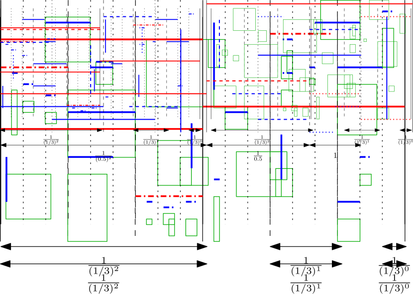
(b) Lines in OPT and line operartions

Figure 3: Horizontal line operations

Claim 5.

Let $\mathrm{DP}(S^{\prime},\mathcal{L})$ be one of the subproblems after applying the operations above. There are at most $\varepsilon^{-3}$ line segments $\mathcal{L}^{\prime}$ (horizontal or vertical) from $\mathrm{OPT}$ of level $j$ that have an endpoint inside $S^{\prime}$.

Consider a resulting subproblem $\mathrm{DP}(S^{\prime\prime},\mathcal{L})$. For each line segment $\ell\in\mathrm{OPT}$ such that $\ell$ crosses $S^{\prime\prime}$, i.e., $S^{\prime\prime}\setminus\ell$ has two connected components, we apply the line operation to the line that contains $\ell$. We apply the trivial operation until it is no longer applicable. In each subproblem $\mathrm{DP}(S^{\prime\prime\prime},\mathcal{L})$ obtained after this step, we apply the add operation to the line segments of level $j$ that have an endpoint in $S^{\prime\prime\prime}$, i.e., to the set $\mathcal{L}^{\prime}:=\{\ell\cap S^{\prime\prime\prime}\mid\ell\in\mathrm{OPT}\wedge\ell\cap S^{\prime\prime\prime}\neq\emptyset\wedge\ell\,\mathrm{is\,of\,level\,}j\}$.

As an example, look at Figure 3, with $\varepsilon=1/3$. The solid lines in it are of level 0, the dashed lines of level 1, and dotted lines of level 2. Also the black lines are vertical grid lines, the blue lines are (well-aligned) lines in $\mathrm{OPT}$ and the red lines are lines along which horizontal line operations are applied. It can be seen from this example that a segment of level $j$, by virtue of it being well-aligned, will get removed by a trivial operation of level less than $j+3$.

2.4 Analysis of DP-decision tree

We want to prove that the resulting tree $T$ is indeed a DP-decision-tree corresponding to a solution of cost at most $(1+\varepsilon)\mathrm{OPT}$. To this end, first we need to show that whenever we apply the add operation to a subproblem $\mathrm{DP}(S,\mathcal{L})$ for a set $\mathcal{L}^{\prime}$ then $|\mathcal{L}|+|\mathcal{L}^{\prime}|\leq 3\varepsilon^{-3}$. The key insight for this is that if we added a line segment $\ell\in\mathrm{OPT}$ of some level $j$, then it will not be included in the respective set $\mathcal{L}$ of later subproblems of level $j+3$ or higher since $\ell$ is well-aligned. More precisely, if $\ell$ is horizontal then its $x$-coordinates are aligned with the grid lines of level $j+3$. Hence, if $\ell$ or a part of $\ell$ is contained in a set $\mathcal{L}$ of some subproblem $\mathrm{DP}(S,\mathcal{L})$ for some level $j+3$, then we applied the trivial operation to $\ell$ and thus $\ell$ “disappeared” from $\mathcal{L}$. If $\ell$ is vertical and it appears in a $\mathrm{DP}(S,\mathcal{L})$ for some level $j+3$ then we applied the line operation to the horizontal lines that contain the two endpoints of $\ell$. Afterwards, we applied the trivial operation to $\ell$ until $\ell$ “disappeared” from $\mathcal{L}$.

In particular, for each subproblem $\mathrm{DP}(S,\mathcal{L})$ constructed by operations of level $j$, the set $\mathcal{L}$ can contain line segments of levels $j-2,j-1$, and $j$; but no line segments of a level $j^{\prime}$ with $j^{\prime}<j-2$. We make this and some other technicalities formal in the proof of the next lemma.

Lemma 6.

The constructed tree $T$ is a DP-decision-tree.

Proof.

We first notice that any reduction in the tree corresponding to a trivial or line operation on $\mathrm{DP}(S,\mathcal{L})$ can only lead to subproblems of the form $\mathrm{DP}(S^{\prime},\mathcal{L}^{\prime})$ with $\mathcal{L}^{\prime}\subseteq\mathcal{L}$. Hence, such reductions cannot lead to a contradiction of any DP-decision tree property.

We now consider the add operations to ensure that any newly created node, by applying the add operation on set $\mathcal{L}^{\prime}:=\{\ell\cap S^{\prime}\mid\ell\in\mathrm{OPT}\wedge\ell\cap S^{\prime}\neq\emptyset\wedge\ell\mathrm{\,is\,of\,level\,}j\}$ to subproblem $\mathrm{DP}(S,\mathcal{L})$, maintains the property that $|\mathcal{L}|\cup|\mathcal{L}^{\prime}|\leq 3\varepsilon^{-3}$. We do this by induction,

Base case:

For the sequence of operations of level $j<3$, we know by Claim 4 and Claim 5 that the ‘added’ set $\mathcal{L}^{\prime}$ always satisfied $|\mathcal{L}^{\prime}|\leq\varepsilon^{-3}$. Since these are the only added sets in the first 3 levels, we can be sure that $|\mathcal{L}|+|\mathcal{L}^{\prime}|\leq 3\varepsilon^{-3}$.

Hypothesis:

We assume that all add operations in the sequence of operations corresponding to level $j-1$, satisfied the property that $|\mathcal{L}|+|\mathcal{L}^{\prime}|\leq 3\varepsilon^{-3}$.

Induction:

Consider an add operation for segments in $\mathrm{OPT}$ of level $j$. Any such operation was preceded by a series of line operations along grid lines of level $j$ and all viable trivial operations. The grid lines of level $j$ are separated by $\varepsilon^{j-2}$ units, and hence any horizontal segment from $\mathrm{OPT}$ in $\mathcal{L}$ of level $j^{\prime}<j-2$ (which have length $\geq\varepsilon^{j-2}$ and being well aligned, completely cut across any cell they intersect) can have the trivial operation applied to them, and be removed from $\mathcal{L}$. Similarly, for vertical segments in $\mathrm{OPT}$ of level $j^{\prime}<j-2$, we explicitly apply the line operation to the horizontal lines that contain its end points, and hence again these also get removed from $\mathcal{L}$ when we apply all possible trivial operations. Thus we are left only with segments added in operations of level $j-1$ and $j-2$ in $\mathcal{L}$. But we know from Claim 5 that at each level we add at most $\varepsilon^{-3}$ segments. Thus application of an add operation at this stage ensures that $|\mathcal{L}|+|\mathcal{L}^{\prime}|\leq 3\varepsilon^{-3}$. ∎

We want to show that the cost of the solution corresponding to $T$ is at most $(1+O(\varepsilon))\mathrm{OPT}$. In fact, depending on the offset $a$ this might or might not be true. However, we show that there is a choice for $a$ such that this is true (in fact, we will show that for a random choice for $a$ the cost will be at most $(1+O(\varepsilon))\mathrm{OPT}$ in expectation). Intuitively, when we apply the line operation to a vertical grid line $\ell$ of some level $j$ then the incurred cost is at most $O(1)$ times the cost of the line segments from $\mathrm{OPT}$ of level $j$ or larger that stab at least one rectangle intersected by $\ell$. A line segment $\ell^{\prime}\in\mathrm{OPT}$ of level $j$ stabs such a rectangle only if $\ell^{\prime}$ is intersected by $\ell$ (if $\ell^{\prime}$ is horizontal) or the $x$-coordinate of $\ell^{\prime}$ is close to $\ell$ (if $\ell^{\prime}$ is vertical). Here we use that $h_{i}\geq w_{i}$ for each rectangle $R_{i}\in\mathrm{OPT}$.

Thus, we want to bound the total cost over all levels $j$ of the line segments from $\mathrm{OPT}$ that are in level $j$ and that are intersected or close to grid lines of level $j$ or smaller. We will show that if we choose $a$ randomly then the total cost of such grid lines is at most $\varepsilon\cdot\mathrm{OPT}$ in expectation. Hence, by using the constant approximation algorithm from [CvDF⁺18] in expectation the total cost due to all line operations for vertical line segments is at most $O(\varepsilon)\cdot\mathrm{OPT}$.

When we apply the line operation for a horizontal line, then the cost of stabbing the corresponding rectangles is at most the width of the rectangle $S$ of the current subproblem $\mathrm{DP}(S,\mathcal{L})$. We will charge this cost to the line segments of $\mathrm{OPT}$ inside $S$ of the current level or higher levels. We will argue that we can charge each such line operation to line segments from $\mathrm{OPT}$ whose total width is at least $1/\varepsilon$ times the width of $S$. This costs another $O(\varepsilon)\cdot\mathrm{OPT}$ in total due to all applications of line operations for horizontal line segments.

The add operation yields a cost of exactly $\mathrm{OPT}$ and the trivial operation does not cost anything. This yields a total cost of $(1+O(\varepsilon))\mathrm{OPT}$.

Formally, we prove this in the following lemma.

Lemma 7.

There is a choice for the offset $a$ such that the solution $\overline{\mathrm{SOL}}([0,n]\times[0,4n^{2}],\emptyset)$ in $T$ has a cost of at most $(1+O(\varepsilon))\mathrm{OPT}$.

Proof.

In the tree as defined above, the add operations are only applied on segments from $\mathrm{OPT}$, and hence the cost across all such add operations is at most $c(\mathrm{OPT})$. Similarly, the trivial operations are applied on segments which were ‘added’ before, and hence their cost is also already accounted for. So we are left with analyzing the cost of stabbing the rectangles which are intersected by the lines along which we apply the line operations. We claim that for a random offset $a$, this cost is $O(\varepsilon\cdot\mathrm{OPT})$, which would give us the required result.

Let us first consider any line operation of level $j$ that is applied to a horizontal line $\ell$. This operation would create 2 cells of width at most $\varepsilon^{j-2}$, one of which either contains $\varepsilon^{-3}$ endpoints of segments (horizontal or vertical) from $\mathrm{OPT}$ of level $j$; or contains at least one vertical segment from $\mathrm{OPT}$ of level $j^{\prime}<j-2$, i.e., the cost of the segments from $\mathrm{OPT}$ with at least one endpoint in this cell is at least $\varepsilon^{-3}\cdot\varepsilon^{j}=\varepsilon^{j-3}$. Since a segment of width $\varepsilon^{j-2}$ (width of cell) is sufficient to stab all rectangles stabbed by $\ell$, we see that this horizontal line takes only $\varepsilon$ times the cost of the segments in $\mathrm{OPT}$ with at least one endpoint in the cell. We charge the cost of this horizontal segment to these corresponding endpoints. Since each such segment in $\mathrm{OPT}$ of level $j$ can be charged at most twice, by summing over all horizontal line operations over all levels we get that the cost of such line operations is at most $2\varepsilon\cdot\mathrm{OPT}$.

Now, let us consider the line operations applied to vertical grid lines. We wish to bound the cost of stabbing all the rectangles intersected or close to grid lines (will be formally defined shortly), over all levels $j$. This as mentioned above can also be stated as bounding the cost, over all levels $j$, of line segments in level $j$ of $\mathrm{OPT}$ (call this set $\mathrm{OPT}_{j}$) intersected or close to grid lines of level $j$ or smaller. For a horizontal segment $\ell\in\mathrm{OPT}_{j}$, let $I_{\ell}$ be the indicator variable representing the event that a grid line of level $j$ or smaller intersects $\ell$ ($I_{\ell}=0$ for vertical segments). Since $|\ell|\leq\varepsilon^{j-1}$, if we take a random offset $a$, we can say that,

$$\mathop{\mathbb{E}}[I_{\ell}]\leq\frac{\varepsilon^{j-1}}{\varepsilon^{j-2}}=\varepsilon.$$

For a vertical segment $\ell\in\mathrm{OPT}_{j}$, let $J_{\ell}$ be the indicator variable representing the event that a grid line of level $j$ or smaller intersect the rectangle stabbed by $\ell$ ($J_{\ell}=0$ for horizontal segments). Since for $j>0$, $|\ell|\leq\varepsilon^{j-1}$, we know that for the rectangle stabbed by $\ell$, the dimensions satisfy $w_{i}\leq h_{i}\leq\varepsilon^{j-1}$. This means that to stab such a rectangle, $\ell$ has to lie close to, i.e., within $\pm\varepsilon^{j-1}$ of the vertical grid line. So for a random offset $a$ and level $j>0$ we can say that:

$$\mathop{\mathbb{E}}[J_{\ell}]\leq\frac{2\varepsilon^{j-1}}{\varepsilon^{j-2}}=2\varepsilon.$$

For level 0, we note that even though the vertical segments can be very long, the maximum width of a rectangle is at most 1. So $\ell$ has to lie within $\pm 1$ of the grid line, giving us:

$$\mathop{\mathbb{E}}[J_{\ell}]\leq\frac{2}{\varepsilon^{-2}}=2\varepsilon^{2}\leq 2\varepsilon.$$

With the expectations computed above, we can upper bound the expected cost of segments in $\mathrm{OPT}$ intersected by vertical line operations as:

$$\mathop{\mathbb{E}}\left[\sum_{j}\sum_{\ell\in\mathrm{OPT}_{j}}(I_{\ell}+J_{\ell})\cdot|\ell|\right] =\sum_{j}\sum_{\ell\in\mathrm{OPT}_{j}}\mathop{\mathbb{E}}\left[(I_{\ell}+J_{\ell})\cdot|\ell|\right]$$

$$=\sum_{j}\sum_{\ell\in\mathrm{OPT}_{j}}|\ell|\cdot(\mathop{\mathbb{E}}[I_{\ell}]+\mathop{\mathbb{E}}[J_{\ell}])$$

$$\leq\sum_{j}\sum_{\ell\in\mathrm{OPT}_{j}}|\ell|\cdot(\varepsilon+2\varepsilon)$$

$$=3\varepsilon\cdot\mathrm{OPT}$$

Now, by using the $\alpha$-approximation algorithm for stabbing from [CvDF⁺18], where $\alpha$ is a constant, the solution returned by our algorithm takes an additional cost of $3\alpha\cdot\varepsilon\cdot\mathrm{OPT}$. ∎

Now we prove our main theorem.

Theorem 8.

There is a $(1+\varepsilon)$-approximation algorithm for the general rectangle stabbing problem with a running time of $(n/\varepsilon)^{O(1/\varepsilon^{3})}$, assuming that $h_{i}\geq w_{i}$ for each rectangle $R_{i}\in\mathcal{R}$.

Proof.

We gave a DP algorithm in Section 2.2 which was shown to have the required running time in Lemma 2. Further in Lemma 7 we showed the correctness and that the solution computed by the DP is actually a $1+O(\varepsilon)$ approximation of the solution. ∎

Theorem 8 has some direct implications. First, it yields a PTAS for the general square stabbing problem.

Corollary 9.

There is a PTAS for the general square stabbing problem.

Also, it yields a $(2+\varepsilon)$-approximation algorithm for the general rectangle stabbing problem for arbitrary rectangles: we can simply split the input into rectangles $R_{i}$ for which $h_{i}\geq w_{i}$ holds, and those for which $h_{i}<w_{i}$ holds, and output the union of these two solutions.

Corollary 10.

There is a $(2+\varepsilon)$-approximation algorithm for the general rectangle stabbing problem with a running time of $(n/\varepsilon)^{O(1/\varepsilon^{3})}$.

Finally, it yields a PTAS for the horizontal rectangle stabbing problem: we can take the input of that problem and stretch all input rectangles vertically such that it is always very costly to stab any rectangle vertically (so in particular our $(1+\varepsilon)$-approximate solution would never do this). Then we apply the algorithm due to Theorem 8.

Corollary 11.

There is a $(1+\varepsilon)$-approximation algorithm for the horizontal rectangle stabbing problem with a running time of $(n/\varepsilon)^{O(1/\varepsilon^{3})}$.

3 $\delta$-large rectangles

We now consider the case of $\delta$-large rectangles for some given constant $\delta$, i.e., where for each input rectangle $R_{i}$ we assume that $w_{i}\leq 1$ and $h_{i}\leq 1$ and additionally $w_{i}\geq\delta$ or $h_{i}\geq\delta$. In other words, none of the rectangles are small ($<\delta$) in both dimensions. For this case we again give a PTAS in which we use our algorithm due to Theorem 8 as a subroutine.

First, by losing only a factor of $1+\varepsilon$, we divide the instance into independent subproblems which are disjoint rectangular cells. For each cell $C_{i}$, we denote by $\mathrm{OPT}(C_{i})$ the cells from $\mathrm{OPT}$ that are contained in $C_{i}$ and our routine ensures that $c(\mathrm{OPT}(C_{i}))\leq O(1/\varepsilon^{3})$. Then for each cell $C_{i}$, the number of segments in $\mathrm{OPT}(C_{i})$ with length longer than $\delta$ is bounded by $O({1}/{\delta\varepsilon^{3}})$. We guess them in polynomial time. Now, the remaining segments in $\mathrm{OPT}$ are all of length smaller than $\delta$, and hence they can stab a rectangle along its shorter dimension. Hence, we can divide the remaining rectangles into two disjoint sets, one with $h_{i}{\geq}w_{i}$ and the other with $w_{i}\geq h_{i}$, and use Theorem 8 to get a $1+\varepsilon$ approximation of the remaining problem. In the following, we describe our algorithm in detail.

3.1 Guessing long segments in the solution

We first start by discretizing the input similar to Lemma 1.

Lemma 12.

By losing a factor $(1+O(\varepsilon))$ in the approximation ratio, we can assume for each $R_{i}\in\mathcal{R}$ the following properties hold:

1. $x_{1}^{(i)},x_{2}^{(i)},y_{1}^{(i)},y_{2}^{(i)}$ are discretized and within $[0,n]$,

2. each line segment in $\mathrm{OPT}$ has width of at most $1/\varepsilon$.

Proof.

We first prove Property $(i)$. Since each rectangle $R_{i}\in\mathcal{R}$ has width $w_{i}\leq 1$, the instance either has some $x$-coordinate that is not covered by any rectangle – in which case we can split the instance into smaller subproblems around this $x$-coordinate – or the total width of the instance is less than $n$. Hence all the $x$-coordinates of the rectangles can be assumed to be between 0 and $n$. Further, we extend the rectangles on both sides to make their $x$-coordinates align with the next nearest multiple of ${\varepsilon}/{n}$ (discretization). Clearly this involves extension by at most ${2\varepsilon}/{n}$ to the width of every rectangle, and at most a $2\varepsilon$ addition to the cost of the solution. We can use the same argument to show that the heights are also discretized and between 0 and $n$, since the heights of all rectangles are also less than 1. The height discretization similarly adds another $2\varepsilon$ to the cost of the solution.

Now we look at Property $(ii)$. Consider any horizontal (resp. vertical) segment $\ell\in\mathrm{OPT}$, that is longer than $1/\varepsilon$. From the left (resp. bottom) end point, we divide the segment into consecutive smaller segments of length $1/\varepsilon-2$ each, with one potential last piece being smaller than $1/\varepsilon-2$. Now, for each smaller segment we extend it on both sides in such a way that it completely stabs the rectangles that it intersects. Since the maximum width (resp. height) of a rectangle is 1, we extend each such segment by at most 2 units.

In the worst case the highest possible fractional increase due to the above division happens when we have a segment of length $1/\varepsilon+\delta$ for very small $\delta>0$. But even in this case the fractional increase in the length of segments in $\mathrm{OPT}$ can be bounded by,

$$\frac{1/\varepsilon+\delta+4}{1/\varepsilon+\delta}=1+4\cdot\frac{1}{1/\varepsilon+\delta}\leq 1+4\varepsilon.\qed$$

Then we continue by constructing vertical grid lines at each $x$-coordinate $a+k\cdot\varepsilon^{-2}$ with $k\in\mathbb{N}$ and a random offset $a\in\mathbb{N}_{0}$. By removing the rectangles that intersect with these grid lines, we divide the input instance into strips of width $1/\varepsilon^{2}$ each. Next, we show that the removed rectangles can be stabbed at very low total cost.

Lemma 13.

Consider the input rectangles that are intersected by vertical grid lines. They can all be stabbed by a set of segments of total expected cost $O(\varepsilon)\cdot\mathrm{OPT}$.

Proof.

Similar to Lemma 7, we wish to bound the cost of stabbing all the rectangles intersected or close to grid lines, which can also be stated as bounding the cost, of line segments of $\mathrm{OPT}$ intersected or close to the grid lines. For a horizontal segment $\ell\in\mathrm{OPT}$, let $I_{\ell}$ be the indicator variable representing the event that a grid line intersects $\ell$ ($I_{\ell}=0$ for vertical segments). Since $|\ell|\leq 1/\varepsilon$, if we take a random offset $a$, we can say that,

$$\mathop{\mathbb{E}}[I_{\ell}]\leq\frac{\varepsilon^{-1}}{\varepsilon^{-2}}=\varepsilon.$$

For a vertical segment $\ell\in\mathrm{OPT}$, let $J_{\ell}$ be the indicator variable representing the event that a grid line intersects the rectangle stabbed by $\ell$ ($J_{\ell}=0$ for horizontal segments). Since the width of all rectangles is less than 1, to stab a rectangle, $\ell$ has to lie close to, i.e., within $\pm 1$ of the vertical grid line. So for a random offset $a$ we can say that,

$$\mathop{\mathbb{E}}[J_{\ell}]\leq\frac{2}{\varepsilon^{-2}}=2\varepsilon^{2}\leq 2\varepsilon.$$

With the expectations computed above, we can upper bound the expected cost of segments in $\mathrm{OPT}$ intersected by vertical line operations as,

$$\mathop{\mathbb{E}}\left[\sum_{\ell\in\mathrm{OPT}}(I_{\ell}+J_{\ell})\cdot|\ell|\right] =\sum_{\ell\in\mathrm{OPT}}\mathop{\mathbb{E}}\left[(I_{\ell}+J_{\ell})\cdot|\ell|\right]$$

$$=\sum_{\ell\in\mathrm{OPT}}|\ell|\cdot(\mathop{\mathbb{E}}[I_{\ell}]+\mathop{\mathbb{E}}[J_{\ell}])$$

$$\leq\sum_{\ell\in\mathrm{OPT}}|\ell|\cdot(\varepsilon+2\varepsilon)$$

$$=3\varepsilon\cdot\mathrm{OPT}$$

Now, by using the $\alpha$-approximate algorithm for HV-Stabbing from [CvDF⁺18], where $\alpha$ is a constant, we can find a set of segments that stabs the set of rectangles intersected by the vertical grid lines with an additional cost of $3\alpha\cdot\varepsilon\cdot\mathrm{OPT}$. ∎

Now we divide these vertical strips into smaller rectangular cells such that the optimal solution for each cell is $O(1/\varepsilon^{3})$.

Lemma 14.

In time $n^{O(1)}$ we can compute a set of horizontal line segments of total cost $O(\varepsilon)\cdot\mathrm{OPT}$ that, together with the vertical grid lines, divides the input instance into rectangular cells containing independent subproblems, each with an optimal solution of cost $O(1/\varepsilon^{3})$.

Proof.

We will consider each vertical strip of width at most $1/\varepsilon^{2}$ separately as they constitute independent subproblems. Consider one such strip. We sweep a horizontal line from bottom to top, and at each discretized $y$-coordinate compute an $\alpha$-approximate solution (using $\alpha$-approximation algorithm of [CvDF⁺18] for HV-Stabbing) for the subproblem completely contained in the cell below the line. At the smallest $y$-coordinate $y_{0}$, at which the cost of the solution exceeds $1/\varepsilon^{3}$, we take the line $[0,1/\varepsilon^{2}]\times y_{0}$ as a part of our solution. Note that by moving the line up by another $\varepsilon/n$, the cost of the solution can increase by at most $1/\varepsilon$, therefore the cost of segments from $\mathrm{OPT}$ in the cell thus created below the line is between $1/(\alpha\varepsilon^{3})$ and $1/\varepsilon^{3}+1/\varepsilon$, which is $\Omega(1/\varepsilon^{3})$.

Thus every time we add a horizontal segment as described above, we add a segment of length $1/\varepsilon^{2}$ to the solution, and create a subproblem which has an optimal solution of cost $\Omega(1/\varepsilon^{3})$. Hence the cost of the added segment is at most $O(\varepsilon^{-2}/\varepsilon^{-3})=O(\varepsilon)$ times the cost of the solution to the subproblem that it creates. Since an optimal solution to all such cells can be at most the cost of the original instance, the cost of the horizontal segments that we have added is at most $O(\varepsilon)\cdot\mathrm{OPT}$. ∎

Now, in the solution to a subproblem contained in a cell as described above, there can be at most $O(1/\delta\varepsilon^{3})$ long segments, i.e., segments of length at least $\delta$. Since there are only a polynomial number of discretized candidate segments we can guess the set of long segments in the solution in polynomial time (the exact analysis is shown later).

3.2 Computing short segments in the solution

For each guess made for the set of long segments in the solution, we compute a $(1+\varepsilon)$-approximation for the short segments, i.e., segments of length at most $\delta$ in the solution using Theorem 8.

Note that any rectangle with both height and width at least $\delta$ will have to be stabbed by a segment longer than $\delta$. However, since all segments in the solution of length at least $\delta$ have already been guessed, each remaining segment can stab a $\delta$-large rectangle only along its shorter dimension. So the rectangles in the instance that have not yet been stabbed can be partitioned into two independent instances, one in which has rectangles with width less than $\delta$ (will be stabbed horizontally) and one which has rectangles with height less than $\delta$ (will be stabbed vertically). We apply Theorem 8 on each of these independent instances and combine the solutions to get a $(1+\varepsilon)$-approximate solution for the remaining problem.

Theorem 15.

For HV-Stabbing with $\delta$-large rectangles, there is a $(1+\varepsilon)$-approximation algorithm with a running time of $(n/\varepsilon)^{O(1/\delta\varepsilon^{3})}$.

Proof.

First, we analyze the running time. In the first phase of the algorithm, we divide the given instance into ${n}/({1/\varepsilon^{2}})=n\varepsilon^{2}$ strips, and run the constant factor $n^{O(1)}$ approximation algorithm from [CvDF⁺18] for each discretized $y$-coordinate. This requires a running time of $n\varepsilon^{2}\times{n}/({\varepsilon/n})\times n^{O(1)}=\varepsilon\cdot n^{O(1)}$. Now in a strip there are at most $({n}/{(\varepsilon/n)})\times({(1/\varepsilon^{2})}/{(\varepsilon/n)})=n^{3}/\varepsilon^{4}$ possible discretized end points for segments, which means there are less than $\binom{n^{3}/\varepsilon^{4}}{2}$, i.e., $O(n^{4}/\varepsilon^{8})$ possible candidate segments in a strip. Hence, we can enumerate over all of their subsets of size $O(1/\delta\varepsilon^{3})$ in $(n/\varepsilon)^{O(1/\delta\varepsilon^{3})}$ time. Following this we have two invocations of Theorem 8 to solve the independent subproblems which would together take $(n/\varepsilon)^{O(1/\varepsilon^{3})}$. This brings the overall running time of the algorithm to be $(n/\varepsilon)^{O(1/\delta\varepsilon^{3})}$.

The correctness of the algorithm follows from the fact that we can correctly guess all the $\delta$-large segments in $\mathrm{OPT}$, and once we have them the remaining problem gets divided into independent subproblems, for each of which we can compute a $(1+\varepsilon)$-approximation. So the approximation factor for the overall algorithm is also $(1+\varepsilon)$. ∎

4 Generalized minimum Manhattan network

In the generalized minimum Manhattan network problem (GMMN), we are given a set $R$ of $n$ unordered terminal pairs, and the goal is to find a minimum-length rectilinear network such that every pair in $R$ is M-connected, that is, connected by an Manhattan-path, which is a path consisting of axis parallel segments whose total length is the Manhattan distance of the pair under consideration.

For the special case of 2D-GMNN, where all terminals lie on a 2 dimensional plane, [DFK⁺18] gave a $O(\log n)$-approximate solution using a $(6+\varepsilon)$-approximate solution for $x$-separated 2D-GMMN instances. An instance of GMMN is called $x$-separated if there is a vertical line that intersects the rectangle formed by any pair of terminals as the diagonally opposite corners of the rectangle. Their algorithm solves a $x$-separated instance by giving a solution of the form $N=A_{\text{up}}\cup A_{\text{down}}\cup S$, where $S$ is a set of horizontal segments stabbing all the rectangles in the instance and $A_{\text{up}}\cup A_{\text{down}}$ is a set of segments of cost bounded by $(2+2\varepsilon)\cdot(\mathrm{OPT}+\mathrm{OPT}_{\text{ver}})$. Using a 4-approximate algorithm for finding the set of segments $S$, horizontally stabbing the rectangles, a bound of $(6+\varepsilon)\cdot\mathrm{OPT}$ is obtained for the cost of segments in $N$. But instead of the 4-approximate algorithm we can instead use the PTAS from Corollary 11 to obtain a better bound of $(4+\varepsilon)\cdot\mathrm{OPT}$ on the cost as follows,

$${c(N)} ={c(A_{\text{up}})}+{c(A_{\text{down}})}+{c(S)}$$

$$\leq(2+2\varepsilon)\cdot(\mathrm{OPT}+\mathrm{OPT}_{\text{ver}})+(1+\varepsilon)\cdot\mathrm{OPT}_{\text{hor}}$$

$$\leq(2+2\varepsilon)\cdot\mathrm{OPT}+(2+2\varepsilon)\cdot(\mathrm{OPT}_{\text{ver}}+\mathrm{OPT}_{\text{hor}})$$

$$=(4+\varepsilon^{\prime})\cdot\mathrm{OPT}.$$

Note that in the above equations $\mathrm{OPT}_{\text{ver}}$ and $\mathrm{OPT}_{\text{hor}}$ refer to the cost of the vertical and horizontal segments respectively in an optimal solution.

References

- [AES10] Boris Aronov, Esther Ezra, and Micha Sharir. Small-size eps-nets for axis-parallel rectangles and boxes. SIAM Journal on Computing, 39(7):3248–3282, 2010.
- [AW13] Anna Adamaszek and Andreas Wiese. Approximation schemes for maximum weight independent set of rectangles. In FOCS, pages 400–409, 2013.
- [BG95] Hervé Brönnimann and Michael T. Goodrich. Almost optimal set covers in finite vc-dimension. Discret. Comput. Geom., 14(4):463–479, 1995.
- [BK14] Nikhil Bansal and Arindam Khan. Improved approximation algorithm for two-dimensional bin packing. In SODA, pages 13–25, 2014.
- [BMSV+09] Luca Becchetti, Alberto Marchetti-Spaccamela, Andrea Vitaletti, Peter Korteweg, Martin Skutella, and Leen Stougie. Latency-constrained aggregation in sensor networks. ACM Transactions on Algorithms (TALG), 6(1):1–20, 2009.
- [BP14] Nikhil Bansal and Kirk Pruhs. The geometry of scheduling. SIAM Journal on Computing, 43(5):1684–1698, 2014.
- [CG14] Timothy M. Chan and Elyot Grant. Exact algorithms and apx-hardness results for geometric packing and covering problems. Comput. Geom., 47(2):112–124, 2014.
- [CGKS12a] Timothy M Chan, Elyot Grant, Jochen Könemann, and Malcolm Sharpe. Weighted capacitated, priority, and geometric set cover via improved quasi-uniform sampling. In Proceedings of the twenty-third annual ACM-SIAM symposium on Discrete Algorithms, pages 1576–1585. SIAM, 2012.
- [CGKS12b] Timothy M. Chan, Elyot Grant, Jochen Könemann, and Malcolm Sharpe. Weighted capacitated, priority, and geometric set cover via improved quasi-uniform sampling. In Yuval Rabani, editor, SODA, pages 1576–1585, 2012.
- [Chv79] Vasek Chvatal. A greedy heuristic for the set-covering problem. Mathematics of operations research, 4(3):233–235, 1979.
- [CKPT17] Henrik I Christensen, Arindam Khan, Sebastian Pokutta, and Prasad Tetali. Approximation and online algorithms for multidimensional bin packing: A survey. Computer Science Review, 24:63–79, 2017.
- [CvDF+18] Timothy M. Chan, Thomas C. van Dijk, Krzysztof Fleszar, Joachim Spoerhase, and Alexander Wolff. Stabbing rectangles by line segments - how decomposition reduces the shallow-cell complexity. In Wen-Lian Hsu, Der-Tsai Lee, and Chung-Shou Liao, editors, ISAAC, volume 123, pages 61:1–61:13, 2018.
- [DFK+18] Aparna Das, Krzysztof Fleszar, Stephen Kobourov, Joachim Spoerhase, Sankar Veeramoni, and Alexander Wolff. Approximating the generalized minimum manhattan network problem. Algorithmica, 80(4):1170–1190, 2018.
- [DJK+21] Max A Deppert, Klaus Jansen, Arindam Khan, Malin Rau, and Malte Tutas. Peak demand minimization via sliced strip packing. In APPROX/RANDOM, volume 207, pages 21:1–21:24, 2021.
- [EGSV21] Friedrich Eisenbrand, Martina Gallato, Ola Svensson, and Moritz Venzin. A QPTAS for stabbing rectangles. CoRR, abs/2107.06571, 2021.
- [FJQS08] Gerd Finke, Vincent Jost, Maurice Queyranne, and András Sebő. Batch processing with interval graph compatibilities between tasks. Discrete Applied Mathematics, 156(5):556–568, 2008.
- [GGA+20] Waldo Gálvez, Fabrizio Grandoni, Afrouz Jabal Ameli, Klaus Jansen, Arindam Khan, and Malin Rau. A tight (3/2+) approximation for skewed strip packing. In APPROX/RANDOM, volume 176, pages 44:1–44:18, 2020.
- [GGH+17] Waldo Gálvez, Fabrizio Grandoni, Sandy Heydrich, Salvatore Ingala, Arindam Khan, and Andreas Wiese. Approximating geometric knapsack via l-packings. In FOCS, pages 260–271, 2017.
- [GGK+21] Waldo Gálvez, Fabrizio Grandoni, Arindam Khan, Diego Ramírez-Romero, and Andreas Wiese. Improved approximation algorithms for 2-dimensional knapsack: Packing into multiple l-shapes, spirals, and more. In SoCG, volume 189, pages 39:1–39:17, 2021.
- [GIK02] Daya Ram Gaur, Toshihide Ibaraki, and Ramesh Krishnamurti. Constant ratio approximation algorithms for the rectangle stabbing problem and the rectilinear partitioning problem. Journal of Algorithms, 43(1):138–152, 2002.
- [GKM+21] Waldo Gálvez, Arindam Khan, Mathieu Mari, Tobias Mömke, Madhusudhan Reddy Pittu, and Andreas Wiese. A (2+)-approximation algorithm for maximum independent set of rectangles. CoRR, abs/2106.00623, 2021.
- [HJPVS14] Rolf Harren, Klaus Jansen, Lars Prädel, and Rob Van Stee. A (5/3+ )-approximation for strip packing. Computational Geometry, 47(2):248–267, 2014.
- [HM85] Dorit S. Hochbaum and Wolfgang Maass. Approximation schemes for covering and packing problems in image processing and vlsi. Journal of the ACM (JACM), 32(1):130–136, 1985.
- [KMSW21] Arindam Khan, Arnab Maiti, Amatya Sharma, and Andreas Wiese. On guillotine separable packings for the two-dimensional geometric knapsack problem. In SoCG, volume 189, pages 48:1–48:17, 2021.
- [KP20] Arindam Khan and Madhusudhan Reddy Pittu. On guillotine separability of squares and rectangles. In APPROX/RANDOM, volume 176, pages 47:1–47:22, 2020.
- [KS06] Sofia Kovaleva and Frits Spieksma. Approximation algorithms for rectangle stabbing and interval stabbing problems. SIAM Journal on Discrete Mathematics, 20(3):748–768, 2006.
- [KS21] Arindam Khan and Eklavya Sharma. Tight approximation algorithms for geometric bin packing with skewed items. In APPROX/RANDOM, volume 207, pages 22:1–22:23, 2021.
- [KSS21] Arindam Khan, Eklavya Sharma, and K.V.N. Sreenivas. Geometry meets vectors: Approximation algorithms for multidimensional packing. CoRR, abs/2106.13951, 2021.
- [Mit21] Joseph S. B. Mitchell. Approximating maximum independent set for rectangles in the plane. CoRR, abs/2101.00326, 2021.
- [MRR15] Nabil H. Mustafa, Rajiv Raman, and Saurabh Ray. Quasi-polynomial time approximation scheme for weighted geometric set cover on pseudodisks and halfspaces. SIAM J. Comput., 44(6):1650–1669, 2015.
- [MW15] Tobias Mömke and Andreas Wiese. A (2+)-approximation algorithm for the storage allocation problem. In ICALP, volume 9134, pages 973–984, 2015.
- [MW20] Tobias Mömke and Andreas Wiese. Breaking the barrier of 2 for the storage allocation problem. In ICALP, volume 168, pages 86:1–86:19, 2020.
- [Var10] Kasturi R. Varadarajan. Weighted geometric set cover via quasi-uniform sampling. In STOC, pages 641–648, 2010.