Abstract

We study the continuum limit of the entanglement Hamiltonian of a sphere for the massless scalar field in its ground state by employing the lattice model defined through the discretisation of the radial direction. In two and three spatial dimensions and for small values of the total angular momentum, we find numerical results in agreement with the corresponding ones derived from the entanglement Hamiltonian predicted by conformal field theory. When the mass parameter in the lattice model is large enough, the dominant contributions come from the on-site and the nearest-neighbour terms, whose weight functions are straight lines.

1 Introduction

The reduced density matrix of a subsystem is a central quantity to study in order to understand the entanglement properties of a quantum state for the spatial bipartition. Denoting by $A$ a spatial subregion and by $\bar{A}$ its complement, under the assumption that the Hilbert space of the system factorises as $\mathcal{H}=\mathcal{H}_{A}\otimes\mathcal{H}_{\bar{A}}$, the reduced density matrix is $\rho_{A}\equiv\textrm{Tr}_{\mathcal{H}_{\bar{A}}}\rho$, where $\rho$ is the density matrix of the entire system. Considering a system in its ground state, the entanglement entropy $S_{A}\equiv-\,\textrm{Tr}_{\mathcal{H}_{A}}(\rho_{A}\log\rho_{A})$ measures the bipartite entanglement in this pure state; hence it has been widely explored during the past two decades [1, 2, 3, 4, 5, 6] (see [7, 8, 9] for reviews). The reduced density matrix can always be written as $\rho_{A}=e^{-K_{A}}/\mathcal{Z}_{A}$, where the constant $\mathcal{Z}_{A}=\textrm{Tr}_{\mathcal{H}_{A}}(e^{-K_{A}})$ guarantees the normalisation condition $\textrm{Tr}_{\mathcal{H}_{A}}\rho_{A}=1$ and the operator $K_{A}$ is the entanglement Hamiltonian (also known as modular Hamiltonian).

In certain relativistic quantum field theories (QFTs) and for some particular choices of states and geometric bipartitions, the entanglement Hamiltonian is given by the integral over $A$ of the energy density multiplied by a suitable weight factor. The most important example has been found by Bisognano and Wichmann [10, 11]: for a Lorentz invariant quantum field theory in the $d+1$ dimensional Minkowski spacetime in its ground state, when $A$ is the half space $x>0$, the entanglement Hamiltonian $K_{A}$ is the boost generator in the $x$-direction.

In conformal field theories (CFTs), this result and the conformal invariance have been employed to obtain other entanglement Hamiltonians. A seminal example is the entanglement Hamiltonian of a sphere $B$ of radius $\mathcal{R}$ for a $d+1$ dimensional CFT in Minkowski spacetime and in its ground state. It reads [12, 13] (see also [14])

$$K_{B}\,=\,\mathcal{R}\int_{B}\beta(r)\,T_{tt}(\boldsymbol{x})\,\textrm{d}^{d}\boldsymbol{x}$$ (1.1)

where the weight function $\beta(r)$ is the following parabola

$$\beta(r)\,\equiv\,2\pi\left[\,\frac{1}{2}\left(1-\frac{r^{2}}{\mathcal{R}^{2}}\,\right)\right].$$ (1.2)

When $d=1$, specific conformal mappings have been constructed to obtain other entanglement Hamiltonians $K_{A}$ in the local form, i.e. written as an the integral over $A$ of the energy density multiplied by the proper weight factor [15, 16, 17].

It is important to understand how these QFT results can be obtained as the continuum limit of the corresponding entanglement Hamiltonians in many-body quantum systems on the lattice. For free fermionic and bosonic systems, the Gaussian nature of the ground state allows to obtain explicit expressions for the entanglement Hamiltonian of a lattice subsystem for a generic number of spatial dimensions $d$ [8, 18, 19, 9, 20]. These lattice operators are characterised by long-range and inhomogeneous couplings [21, 22, 23]. In the special case of $d=1$, the continuum limit of the entanglement Hamiltonian of a block made by consecutive sites in a chain of free fermions in the ground state has been studied analytically in [24] by employing the results of [22], finding the parabolic weight function (1.2) expected from CFT. In a massless harmonic chain, the corresponding analysis has been performed numerically in [21, 25].

The entanglement Hamiltonians of a block of consecutive sites have been studied numerically also for non-critical chains in their ground state, finding also in these cases that the entanglement Hamiltonian matrices contain long-range and inhomogeneous couplings. Far away from criticality, a triangular profile for the weight function has been observed [26], which has been understood through the analytic expressions derived for the entanglement Hamiltonian of the half infinite chain [27, 28].

In this manuscript we consider the entanglement Hamiltonian of a sphere $B\in\mathbb{R}^{d}$, mainly focussing on the CFT given by the massless scalar field in the $d+1$ dimensional Minkowski spacetime and in its ground state. We study the continuum limit that leads to the entanglement Hamiltonian $K_{B}$ of the sphere given by (1.1) and (1.2) specialised to this model. Our analysis is mostly numerical and it is based on the method developed in [21, 22, 24, 25] for $d=1$. In the special case of $d=1$, we recover the results for the entanglement Hamiltonian of a segment at the beginning of the semi-infinite line with Dirichlet boundary conditions obtained in [25]. In the massive regime, we adapt to the higher dimensional case of the sphere the analysis made in [26] for the entanglement Hamiltonian of the segment in the massive harmonic chain on the infinite line.

The layout of this paper is as follows. In Sec. 2 we introduce the model of the massive scalar field, the lattice regularisations of its Hamiltonian along the radial direction, the CFT prediction for the entanglement Hamiltonian of the sphere (1.1) for this model and the corresponding expressions on the lattice employed in our numerical analysis. In Sec. 3 we focus on the massless case and study numerically the continuum limit of the entanglement Hamiltonian. In Sec. 4 we discuss the regime where the mass parameter in the lattice model is large. Conclusions are drawn in Sec. 5. In the appendices A and B we report further results that clarify and support some discussions in the main text.

2 Entanglement Hamiltonian of a sphere for the scalar field

In this section we introduce the main expressions employed in this manuscript to study the entanglement Hamiltonian of a sphere in the $d+1$ dimensional Minkowski spacetime for the scalar field in its ground state. In Sec. 2.1 we briefly review the Hamiltonian of the scalar field and its lattice regularisation along the radial direction, as done by Srednicki [2] to study the entanglement entropy of a sphere. In Sec. 2.2 we combine the result of this analysis with the expression for the entanglement Hamiltonian of a generic region in harmonic lattices found by Casini and Huerta [9].

2.1 Hamiltonian and radial regularisations

The Hamiltonian of the massive real scalar field in the $d+1$ dimensional Minkowski spacetime reads

$$H=\frac{1}{2}\int_{\mathbb{R}^{d}}\Big{(}\Pi^{2}-\Phi\,\Delta\Phi+m^{2}\,\Phi^{2}\,\Big{)}\textrm{d}^{d}\boldsymbol{x}$$ (2.1)

where $\boldsymbol{x}\in\mathbb{R}^{d}$ is the vector identifying the spatial position, $\Delta$ denotes the $d$-dimensional Laplacian, $\Phi=\Phi(\boldsymbol{x})$ is the real scalar field and $\Pi=\Pi(\boldsymbol{x})$ its canonically conjugate momentum field. In order to study the entanglement Hamiltonian $K_{B}$ of a sphere $B$, it is convenient to employ the hyperspherical polar coordinates of $\mathbb{R}^{d}$ with origin in the center of the sphere. These coordinates are given by the radial coordinate $r=|\boldsymbol{x}|=\sqrt{x_{1}^{2}+\dots+x_{d}^{2}}\geqslant 0$ and by the vector $\boldsymbol{\Omega}=(\phi,\theta_{1},\dots,\theta_{d-2})$ collecting all the angular coordinates of the $d-1$ dimensional unit sphere $\mathbb{S}$.

In these hyperspherical polar coordinates, the metric reads $\textrm{d}s^{2}=-\,\textrm{d}t^{2}+\textrm{d}r^{2}+r^{2}\,\textrm{d}\boldsymbol{\Omega}^{2}$ and the corresponding volume element to employ in (2.1) is $\textrm{d}^{d}\boldsymbol{x}=r^{d-1}\textrm{d}r\,\textrm{d}\boldsymbol{\Omega}$, where $\textrm{d}\boldsymbol{\Omega}$ is the volume element of $\mathbb{S}$. The Laplacian operator $\Delta$ reads $\Delta=\partial_{r}^{2}+\tfrac{d-1}{r}\;\partial_{r}+\tfrac{1}{r^{2}}\,\tilde{\Delta}$, where $\tilde{\Delta}$ is the spherical Laplace operator in $d-1$ dimensions, whose eigenfunctions are the real spherical harmonics in $d$ dimensions $Y_{\boldsymbol{l}}(\boldsymbol{\Omega})$ of degree $l$ (see e.g. chapter XI in [29] or [30, 31])

$$\tilde{\Delta}\,Y_{\boldsymbol{l}}(\boldsymbol{\Omega})=\lambda_{d}(l)\,Y_{\boldsymbol{l}}(\boldsymbol{\Omega})\;\;\;\qquad\;\;\;\lambda_{d}(l)\equiv\,-\,l\big{(}l+d-2\big{)}$$ (2.3)

where $\boldsymbol{l}=(l,i)$ with $l\geqslant 0$ and $1\leqslant i\leqslant N_{d,l}$ labels the linearly independent spherical harmonics of degree $l$ whose total number is

$$N_{d,l}=\left\{\begin{array}[]{ll}1&l=0\\ \rule{0.0pt}{22.76228pt}\displaystyle\binom{\,l+d-1\,}{l}-\binom{\,l+d-3\,}{l-2}\,=\,\frac{2l+d-2}{l}\,\binom{\,l+d-3\,}{l-1}&l>0\end{array}\right.$$ (2.4)

which can be obtained from the degeneracy of the $SO(d)$ representations.

The entanglement entropy of a sphere for the massless scalar field has been first studied by Srednicki in [2]. Following his analysis, we decompose the fields in (2.1) as

$$\Phi(r,\boldsymbol{\Omega})\,=\,r^{-\frac{d-1}{2}}\sum_{\boldsymbol{l}}\Phi_{\boldsymbol{l}}(r)\;Y_{\boldsymbol{l}}(\boldsymbol{\Omega})\;\;\;\;\qquad\;\;\;\;\Pi(r,\boldsymbol{\Omega})\,=\,r^{-\frac{d-1}{2}}\sum_{\boldsymbol{l}}\Pi_{\boldsymbol{l}}(r)\;Y_{\boldsymbol{l}}(\boldsymbol{\Omega})$$ (2.5)

where the sums can be written as $\sum_{\boldsymbol{l}}(\dots)=\sum_{l=0}^{\infty}\sum_{i=1}^{N_{d,l}}(\dots)$.

In the special case of $d=1$, the scalar field is on the half-line $r\geqslant 0$ and the angular coordinates $\boldsymbol{\Omega}$ do not occur; hence the decomposition in (2.5) becomes trivial. Instead, when either $d=2$ or $d=3$, where we have respectively $N_{2,l}=2$ and $N_{3,l}=2l+1$, the decomposition of $\Phi$ in (2.5) reads respectively

$$\Phi(r,\theta)=\Phi_{0}(r)+\sum_{l>0}\left(\Phi_{l}(r)\,e^{il\theta}+\Phi_{-l}(r)\,e^{-il\theta}\right)\qquad\Phi(r,\theta_{1},\theta_{2})=\sum_{l\geqslant 0}\sum_{m=-l}^{l}\Phi_{l,m}(r)\,Y_{l,m}(\theta,\phi)\,.$$ (2.6)

By employing the orthonormality condition $\int_{\mathbb{S}}Y_{\boldsymbol{l}_{1}}(\boldsymbol{\Omega})\,Y_{\boldsymbol{l}_{2}}(\boldsymbol{\Omega})\,\textrm{d}\boldsymbol{\Omega}\,=\delta_{\boldsymbol{l}_{1},\boldsymbol{l}_{2}}\,$ for the spherical harmonics, one finds that the partial wave components $\Phi_{\boldsymbol{l}}(r)$ and $\Pi_{\boldsymbol{l}}(r)$ in (2.5) are

$$\Phi_{\boldsymbol{l}}(r)\,=\,r^{\frac{d-1}{2}}\!\int_{\mathbb{S}}\Phi(r,\boldsymbol{\Omega})\;Y_{\boldsymbol{l}}(\boldsymbol{\Omega})\,\textrm{d}\boldsymbol{\Omega}\;\;\;\;\qquad\;\;\;\;\Pi_{\boldsymbol{l}}(r)\,=\,r^{\frac{d-1}{2}}\!\int_{\mathbb{S}}\Pi(r,\boldsymbol{\Omega})\;Y_{\boldsymbol{l}}(\boldsymbol{\Omega})\,\textrm{d}\boldsymbol{\Omega}\,.$$ (2.7)

These fields obey the canonical commutation relations

$$\big{[}\Phi_{\boldsymbol{l}_{1}}(r_{1}),\Pi_{\boldsymbol{l}_{2}}(r_{2})\big{]}=\textrm{i}\,\delta_{\boldsymbol{l}_{1},\boldsymbol{l}_{2}}\,\delta(r_{1}-r_{2})\,.$$ (2.8)

We remark that, for any $\boldsymbol{l}$, the fields (2.7) satisfy Dirichlet boundary conditions at $r=0$. This is a crucial feature in our analysis.

By employing (2.3) and the decompositions (2.5) in the Hamiltonian (2.1), it becomes

$$H=\sum_{\boldsymbol{l}}H_{\boldsymbol{l}}\;\;\;\qquad\;\;\;H_{\boldsymbol{l}}\,\equiv\int_{0}^{\infty}\!\widetilde{T}_{tt}^{(\boldsymbol{l})}\,\textrm{d}r$$ (2.9)

where

$$\widetilde{T}_{tt}^{(\boldsymbol{l})}\equiv\frac{1}{2}\,\bigg{\{}\,\Pi_{\boldsymbol{l}}^{2}-\Phi_{\boldsymbol{l}}\,\partial_{r}^{2}\Phi_{\boldsymbol{l}}+\left(\frac{\mu_{d}(l)}{r^{2}}+m^{2}\right)\Phi_{\boldsymbol{l}}^{2}\,\bigg{\}}$$ (2.10)

with $\mu_{d}(l)$ defined in terms of $\lambda_{d}(l)$ introduced in (2.3) as follows

$$\mu_{d}(l)\,\equiv\,\frac{(d-3)(d-1)}{4}-\lambda_{d}(l)\,.$$ (2.11)

From (2.9) and the fact that the fields (2.7) corresponding to different $\boldsymbol{l}$’s commute, one concludes that the ground state of $H$ is the direct product of the ground states of $H_{\boldsymbol{l}}$ for different $\boldsymbol{l}$’s [2]. When $d=1$, only $l=0$ is allowed; hence the coefficient (2.11) vanishes and the sum in (2.9) contains a single term. In this case (2.10) becomes the energy density for the scalar field on the half-line satisfying Dirichlet boundary conditions at the beginning of the half-line [32].

Following the regularisation procedure discussed in [2] (see also [1]), the ultraviolet divergences are regularised by introducing a discretisation of the radial direction (with lattice spacing $a$) and the infrared ones by confining the system into a finite volume; hence we consider a large but finite number $R_{\textrm{\tiny tot}}$ of sites along the discretised radial direction. At the $j$-th site of the discretised radial direction, the position operator $\hat{q}_{\boldsymbol{l},j}$ and the momentum operator $\hat{p}_{\boldsymbol{l},j}$ are dimensionless, Hermitian and satisfy the canonical commutation relations $\big{[}\hat{q}_{\boldsymbol{l}_{1},i}\,,\,\hat{p}_{\boldsymbol{l}_{2},j}\big{]}=\textrm{i}\,\delta_{\boldsymbol{l}_{1},\boldsymbol{l}_{2}}\,\delta_{i,j}$.

In the continuum limit $a\to 0$ and $R_{\textrm{\tiny tot}}\to\infty$. Since we keep $R_{\textrm{\tiny tot}}a=\mathcal{R}_{\textrm{\tiny tot}}$ finite in this limit, the system in the continuum is enclosed within the finite sphere of radius $\mathcal{R}_{\textrm{\tiny tot}}$. The radial position corresponds to $r=ja$, with $0\leqslant r\leqslant\mathcal{R}_{\textrm{\tiny tot}}$, and the fields $\Phi_{\boldsymbol{l}}(r)$ and $\Pi_{\boldsymbol{l}}(r)$ in the continuum limit (which vanish identically for $r>\mathcal{R}_{\textrm{\tiny tot}}$ [2]) can be introduced through the position and momentum operators in the standard way

$$\hat{q}_{\boldsymbol{l},j}\,\longrightarrow\,\Phi_{\boldsymbol{l}}(r)\;\;\qquad\;\;\hat{p}_{\boldsymbol{l},j}\,\longrightarrow\,a\,\Pi_{\boldsymbol{l}}(r)\,.$$ (2.12)

The lattice regularisation defined above leads to $(\hat{q}_{\boldsymbol{l},j+1}+\hat{q}_{\boldsymbol{l},j-1}-2\hat{q}_{\boldsymbol{l},j})/a^{2}$ for the regularisation of $\partial_{r}^{2}\Phi_{\boldsymbol{l}}$. Thus, for the lattice regularisation $\widehat{H}_{\boldsymbol{l}}$ of the operator $H_{\boldsymbol{l}}$ in (2.9) we find

$$\widehat{H}_{\boldsymbol{l}}\,=\,\frac{1}{2a}\,\Big{(}\boldsymbol{\hat{p}}^{\textrm{t}}_{\boldsymbol{l}}\,\boldsymbol{I}_{\textrm{\tiny tot}}\,\boldsymbol{\hat{p}}_{\boldsymbol{l}}+\boldsymbol{\hat{q}}^{\textrm{t}}_{\boldsymbol{l}}\,M_{l}\,\boldsymbol{\hat{q}}_{\boldsymbol{l}}\Big{)}$$ (2.13)

where $\boldsymbol{\hat{p}}_{\boldsymbol{l}}$ and $\boldsymbol{\hat{q}}_{\boldsymbol{l}}$ are the vectors whose $j$-th element is given by $\hat{p}_{\boldsymbol{l},j}$ and $\hat{q}_{\boldsymbol{l},j}$ respectively. The matrix $\boldsymbol{I}_{\textrm{\tiny tot}}$ is the $R_{\textrm{\tiny tot}}\times R_{\textrm{\tiny tot}}$ identity matrix and $M_{l}$ is the $R_{\textrm{\tiny tot}}\times R_{\textrm{\tiny tot}}$ real, symmetric, positive definite and tri-diagonal matrix whose non vanishing entries are

$$\big{(}M_{l}\big{)}_{j,j}=\,2+\frac{\mu_{d}(l)}{j^{2}}+\omega^{2}\;\;\;\qquad\;\;\;\big{(}M_{l}\big{)}_{j,j+1}=\,-1$$ (2.14)

where $\mu_{d}(l)$ has been defined in (2.11), the addition term $2$ in $(M_{l})_{j,j}$ comes from the discretisation of $\Phi_{\boldsymbol{l}}\,\partial_{r}^{2}\Phi_{\boldsymbol{l}}$ and $\omega$ corresponds to the mass parameter in the lattice along the radial direction, which is related to the mass parameter $m$ occurring in the Hamiltonian (2.1) in the continuum limit as $\omega/a\,\longrightarrow\,m$. Since $\mu_{d}(l)$ is quadratic in the parameters $d$ and $l$ and the coefficients of $d^{2}$ and $l^{2}$ are both positive, the large $l$ regime at given $d$ is similar to the regime given by large $d$ with $l$ fixed.

The ground state correlators $\langle\hat{q}_{\boldsymbol{l},i}\,\hat{q}_{\boldsymbol{l},j}\rangle$ and $\langle\hat{p}_{\boldsymbol{l},i}\,\hat{p}_{\boldsymbol{l},j}\rangle$ provide the elements of the $R_{\textrm{\tiny tot}}\times R_{\textrm{\tiny tot}}$ correlation matrices $Q_{l}$ and $P_{l}$ respectively, which can be obtained from (2.14) as [1, 2, 33, 34, 35]

$$Q_{l}\,\equiv\,\frac{1}{2}\,M_{l}^{-1/2}\;\;\;\qquad\;\;P_{l}\,\equiv\,\frac{1}{2}\,M_{l}^{1/2}\,.$$ (2.15)

These correlation matrices are well defined when $\omega=0$, for any $d\geqslant 1$ and $l\geqslant 0$. In particular, since translation invariance does not occur in the lattice model along the radial direction, we do not have to deal with the zero mode. We checked numerically that, when $\mu_{d}(l)=0$ in (2.14) and for large values of $R_{\textrm{\tiny tot}}$, the elements of the correlation matrices (2.15) agree with the analytical expressions for the correlators on the half line with Dirichlet boundary condition at the origin of the half-line given in [36] for $\omega=0$ and in [25] for a generic $\omega\geqslant 0$ (see [37] for the corresponding correlators for the harmonic chain on the line, where the zero mode occurs). In the appendix A we compare (2.15) when $\omega=0$ with the corresponding expressions obtained in the continuum through quantum field theory methods [38, 39].

Various discretisations of the Hamiltonian of the real scalar field have been introduced to study the entanglement entropy of the sphere [2, 40, 41, 42, 43, 44, 45, 46, 47, 48]. We have employed the one characterised by (2.14) (see e.g. also [49]). In the appendix A, the correlators (2.15) corresponding to the matrix $M_{l}$ obtained through a different discretisation are also discussed [2, 40, 42].

2.2 Entanglement Hamiltonian of a sphere

We consider the spatial bipartition of $\mathbb{R}^{d}$ given by a sphere $B$ of radius $\mathcal{R}$ and its complement in the $d+1$ dimensional Minkowski spacetime at any given time slice. When the system is a CFT in its ground state, the entanglement Hamiltonian $K_{B}$ is (1.1), which has been obtained in [12, 13] through a conformal transformation of the entanglement Hamiltonian found by Bisognano and Wichmann [10, 11].

In the special case of the free massless scalar field, $K_{B}$ is (1.1) with $T_{tt}$ given by the integrand of (2.1) when $m=0$. In the resulting $K_{B}$, we can straightforwardly adapt the steps that have led to write (2.1) as (2.9), finding that

$$K_{B}=\sum_{\boldsymbol{l}}K_{B,\boldsymbol{l}}$$ (2.16)

where

$$K_{B,\boldsymbol{l}}\,\equiv\,\mathcal{R}\int_{0}^{\mathcal{R}}\!\!\beta(r)\,\widetilde{T}_{tt}^{(\boldsymbol{l})}\,\textrm{d}r$$ (2.17)

with $\beta(r)$ being defined as the parabola (1.2) and the operator $\widetilde{T}_{tt}^{(\boldsymbol{l})}$ by (2.10) with $m=0$.

In the regularised model obtained by discretising the radial direction and described in Sec. 2.1), the sphere $B$ has radius $R<R_{\textrm{\tiny tot}}$. In the continuum limit, $a\to 0$ and $R\to+\infty$ with $Ra=\mathcal{R}$ fixed. The reduced correlation matrices $Q_{l,B}$ and $P_{l,B}$ at a given value of the angular momentum parameter $l$ are the $R\times R$ symmetric and positive definite matrices obtained by restricting the corresponding correlation matrices in (2.15) to the sites identifying the sphere $B$ along the radial direction, i.e. $(Q_{l,B})_{i,j}=(Q_{l})_{i,j}$ and $(P_{l,B})_{i,j}=(P_{l})_{i,j}$ with $1\leqslant i\leqslant R$ and $1\leqslant j\leqslant R$.

The reduced correlation matrices $Q_{l,B}$ and $P_{l,B}$ at given $l$ provide the reduced covariance matrix $Q_{l,B}\oplus P_{l,B}$ at fixed $l$, whose symplectic spectrum $\{\sigma_{l,k}\,;1\leqslant k\leqslant R\}$ is given by the eigenvalues of $\sqrt{Q_{l,B}\,P_{l,B}}$, which are the same ones of its transpose $\sqrt{P_{l,B}\,Q_{l,B}}$. The uncertainty principle implies that $\sigma_{l,k}>1/2$. Since the ground state of this model is Gaussian and the operators associated to different $\boldsymbol{l}$’s commute, the symplectic spectra of the covariance matrices $Q_{l,B}\oplus P_{l,B}$ at fixed $l$ corresponding to different values of $l$ give the Rényi entropies and the entanglement entropy (see (3.30) and the corresponding discussion).

The Gaussian nature of the ground state, combined with the fact that operators corresponding to different $\boldsymbol{l}$’s commute, leads to the entanglement Hamiltonian $\widehat{K}_{B}=\sum_{\boldsymbol{l}}\widehat{K}_{B,\boldsymbol{l}}$ in the regularised model, where $\widehat{K}_{B,\boldsymbol{l}}$ can be obtained through the results obtained in [18, 8, 9, 20]. In particular, the contribution to $\widehat{K}_{B}$ of the degrees of freedom associated to the sector labelled by $\boldsymbol{l}$ is given by the following quadratic operator [9]

$$\widehat{K}_{\boldsymbol{l},B}=\frac{1}{2}\,\boldsymbol{\hat{u}}_{\boldsymbol{l},B}^{\textrm{t}}\,H_{l,B}\,\boldsymbol{\hat{u}}_{\boldsymbol{l},B}\hskip 14.22636pt\qquad\hskip 14.22636pt\boldsymbol{\hat{u}}_{\boldsymbol{l},B}\equiv\bigg{(}\begin{array}[]{c}\boldsymbol{\hat{q}}_{\boldsymbol{l}}\\ \boldsymbol{\hat{p}}_{\boldsymbol{l}}\end{array}\bigg{)}\bigg{|}_{B}$$ (2.18)

where $H_{l,B}$ is the symmetric, positive definite and block diagonal matrix defined in terms of the reduced correlation matrices $Q_{l,B}$ and $P_{l,B}$ at fixed $l$ as follows

$$H_{l,B}\,\equiv\,V^{(l)}\oplus T^{(l)} \equiv \Big{(}h\big{(}\sqrt{P_{l,B}\,Q_{l,B}}\,\big{)}\oplus h\big{(}\sqrt{Q_{l,B}\,P_{l,B}}\,\big{)}\Big{)}\big{(}P_{l,B}\oplus Q_{l,B}\big{)}$$

$$= \big{(}P_{l,B}\oplus Q_{l,B}\big{)}\Big{(}h\big{(}\sqrt{Q_{l,B}\,P_{l,B}}\,\big{)}\oplus h\big{(}\sqrt{P_{l,B}\,Q_{l,B}}\,\big{)}\Big{)}$$

with

$$h(y)\equiv\frac{1}{y}\,\log\!\left(\frac{y+1/2}{y-1/2}\right).$$ (2.20)

The symplectic spectrum of $H_{l,B}$ in (2.2) gives the single particle entanglement energies $\varepsilon_{l,k}$ at given $l$ (hence $\varepsilon^{2}_{l,k}$ are the eigenvalues of $V^{(l)}\,T^{(l)}$), which are related to the symplectic eigenvalues of $Q_{l,B}\oplus P_{l,B}$ as $\varepsilon_{l,k}=2\,\textrm{arccoth}(2\sigma_{l,k})=\log[(\sigma_{l,k}+1/2)/(\sigma_{l,k}-1/2)]$, whose inverse is $\sigma_{l,k}=\tfrac{1}{2}\coth(\varepsilon_{l,k}/2)$. Notice that both $\sigma_{l,k}$ and $\varepsilon_{l,k}$ depend also on $d$ through (2.14).

3 Continuum limit of the entanglement Hamiltonian at $\omega=0$

In this section we study the entanglement Hamiltonian $K_{B}$ of a sphere $B\in\mathbb{R}^{d}$ for the free massless scalar field by taking the continuum limit of the corresponding entanglement Hamiltonian $\widehat{K}_{B}$ in the regularised model, whose contribution for a given $\boldsymbol{l}$ is (2.18) at $\omega=0$. The expected result is the CFT expression (1.1) specialised to the free massless scalar field, which can be written as in (2.16), in terms of the operator (2.10) with $m=0$. In the resulting CFT expression a non trivial $r$ dependent term occurs whose coefficient (2.11) depends both on $d$ and $l$. This coefficient vanishes identically when $d=1$. In our numerical analysis we follow the procedure employed in [21, 22, 24, 25] for free bosonic and fermionic chains (i.e. for $d=1$) at criticality and in their ground states to study the entanglement Hamiltonians of an interval either on the infinite line [21, 22, 24, 25] or at the beginning of the half-line with Dirichlet boundary conditions at the origin [25].

Plugging the matrix (2.2) into (2.18), one finds that the operator $\widehat{K}_{\boldsymbol{l},B}$ can be written as

$$\widehat{K}_{\boldsymbol{l},B}=\frac{1}{2}\Big{(}\widehat{H}_{T,\boldsymbol{l}}+\widehat{H}_{V,\boldsymbol{l}}\Big{)}$$ (3.1)

where the operators $\widehat{H}_{T,\boldsymbol{l}}$ and $\widehat{H}_{V,\boldsymbol{l}}$ are defined through the symmetric matrices $T^{(l)}$ and $V^{(l)}$ as follows

$$\widehat{H}_{T,\boldsymbol{l}}\equiv\sum_{i,j=1}^{R}T^{(l)}_{i,j}\,\hat{p}_{\boldsymbol{l},i}\,\hat{p}_{\boldsymbol{l},j}\;\;\;\;\qquad\;\;\;\;\widehat{H}_{V,\boldsymbol{l}}\equiv\sum_{i,j=1}^{R}V^{(l)}_{i,j}\,\hat{q}_{\boldsymbol{l},i}\,\hat{q}_{\boldsymbol{l},j}\,.$$ (3.2)

These sums can be organised in various ways, as discussed in [25] for $d=1$. We find it convenient to write the sums in (3.2) by decomposing the contribution coming from the $i$-th row of the matrices $V^{(l)}$ and $T^{(l)}$, as also done in [21, 25] in the case of $d=1$. This choice leads to

$$\widehat{H}_{T,\boldsymbol{l}} = R\sum_{i=1}^{R}\left(\frac{T^{(l)}_{i,i}}{R}\,\hat{p}_{\boldsymbol{l},i}^{2}+\sum_{k=1}^{R-i}\frac{T^{(l)}_{i,i+k}}{R}\;\hat{p}_{\boldsymbol{l},i}\,\hat{p}_{\boldsymbol{l},i+k}+\sum_{k=1}^{i-1}\frac{T^{(l)}_{i,i-k}}{R}\;\hat{p}_{\boldsymbol{l},i}\,\hat{p}_{\boldsymbol{l},i-k}\right)$$ (3.3)

$$\rule{0.0pt}{28.45274pt}\widehat{H}_{V,\boldsymbol{l}} = R\sum_{i=1}^{R}\left(\frac{V^{(l)}_{i,i}}{R}\,\hat{q}_{\boldsymbol{l},i}^{2}+\sum_{k=1}^{R-i}\frac{V^{(l)}_{i,i+k}}{R}\;\hat{q}_{\boldsymbol{l},i}\,\hat{q}_{\boldsymbol{l},i+k}+\sum_{k=1}^{i-1}\frac{V^{(l)}_{i,i-k}}{R}\;\hat{q}_{\boldsymbol{l},i}\,\hat{q}_{\boldsymbol{l},i+k}\right).$$ (3.4)

Following the analysis made in [22, 25] for $d=1$, we conjecture the existence of the limits

$$\lim_{R\to\infty}\frac{T^{(l)}_{i,i+\eta k}}{R}\,\equiv\,\tau_{l,\eta k}(r_{\eta k})\;\;\;\qquad\;\;\;\lim_{R\to\infty}\frac{V^{(l)}_{i,i+\eta k}}{R}\,\equiv\,\nu_{l,\eta k}(r_{\eta k})$$ (3.5)

where $k\geqslant 0$ and $\eta=\pm 1$ are discrete parameters and

$$r_{\tilde{k}}\equiv\frac{1}{R}\bigg{(}i+\frac{\tilde{k}}{2}\,\bigg{)}\,.$$ (3.6)

Notice that $i\pm k/2$ in (3.5) corresponds to the midpoint between the $i$-th and the $(i\pm k)$-th site along the discretised radial direction. Since $T^{(l)}$ and $V^{(l)}$ are symmetric matrices, their diagonals labelled by $+k$ and $-k$ in (3.5) contain the same elements.

In our numerical analyses we considered lattices along the radial direction made by $R_{\textrm{\tiny tot}}\in\{200,\,400,\,600,\,800\}$ and kept $R/R_{\textrm{\tiny tot}}\ll 1$ fixed (we choose $R/R_{\textrm{\tiny tot}}=1/10$). This choice is imposed by the fact that the continuum result that we are studying holds in the limit where the volume of the space is infinite. As already remarked in previous studies on entanglement Hamiltonians in free chains [21, 22, 25], high numerical precision is usually needed. In our case, they are required to evaluate (2.2) because many symplectic eigenvalues of $Q_{l,B}\oplus P_{l,B}$ are very close to $1/2$ and they must be distinguished from $1/2$ in order to be employed in (2.20). Higher precision is needed as $l$ or $d$ or $\omega$ increases. Thus, for $d=2$ and $d=3$ we have restricted our numerical analysis to $l\leqslant 10$ and $\omega\leqslant 5$, working up to a precision of 2000 digits for the highest values of these parameters.

In Fig. 1 and Fig. 2 we show some numerical results for the elements in and near the main diagonals of the matrices $T^{(l)}$ and $V^{(l)}$ when $\omega=0$. From previous analyses for $d=1$ [25, 26], they are expected to be extensive; hence we consider $T^{(l)}_{i,i+k}/R$ and $V^{(l)}_{i,i+k}/R$ (only the data corresponding to $k\in\{0,1,2,3\}$ are reported). The data points in Fig. 1 and Fig. 2 display good collapse close to the boundary of the sphere $B$ as $R$ increases. For small values of $l$, this agreement is observed almost all over the range of the spatial index except near the center of the sphere. These data collapses provide some numerical support to the conjecture (3.5) for small values of $l$. Comparing the left and the right panels in Fig. 1 and Fig. 2, we do not find significant differences between $d=2$ and $d=3$. As $l$ increases, we expect that larger values of $R$ are needed to observe good collapses of the data points. This lack of convergence for high values of $l$ and our limited capability to treat numerically large systems forces us to focus only on small values of $l$.

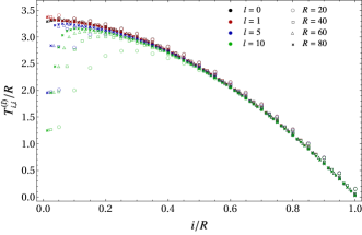
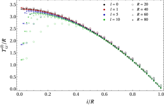
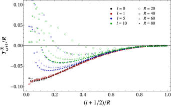
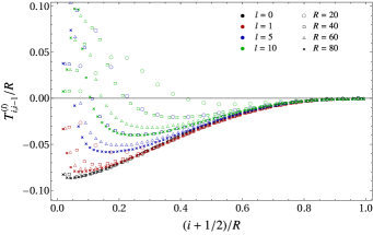
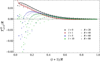
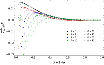
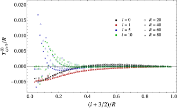
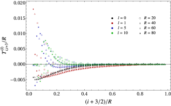
Figure 1: Short-range couplings in the matrix $T^{(l)}/R$ (see (3.2) and (3.5)) when $\omega=0$ and either $d=2$ (left panels) or $d=3$ (right panels), for some small $l$’s and different sizes $R$.

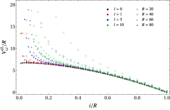
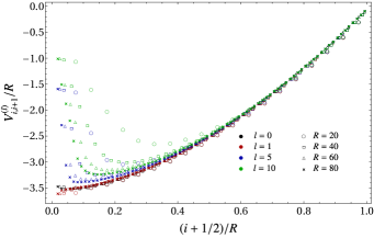
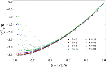
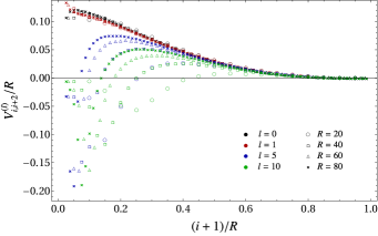
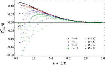
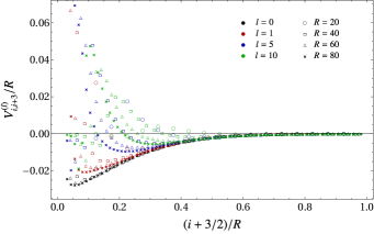
Figure 2: Short-range couplings in the matrix $V^{(l)}/R$ (see (3.2) and (3.5)) when $\omega=0$ and either $d=2$ (left panels) or $d=3$ (right panels), for some small $l$’s and different sizes $R$.

We consider the continuum limit given by $a\to 0$, $R\to\infty$ and $R_{\textrm{\tiny tot}}\to\infty$, while $Ra\equiv\mathcal{R}$ and $R_{\textrm{\tiny tot}}a\equiv\mathcal{R}_{\textrm{\tiny tot}}$ are kept fixed (hence $R/R_{\textrm{\tiny tot}}$ is fixed as well). The parameters $\mathcal{R}$ and $\mathcal{R}_{\textrm{\tiny tot}}$ are the radii respectively of the sphere $B$ and of the entire system, which is a larger concentric sphere.

In the continuum, the radial position is labelled by $r=ia$ with $0<r<\mathcal{R}$. This leads to write (3.6) also as

$$r_{\tilde{k}}=\frac{r}{\mathcal{R}}+\frac{\tilde{k}a/2}{\mathcal{R}}$$ (3.7)

which suggests to expand $\tau_{l,\eta k}$ and $\nu_{l,\eta k}$ in (3.5) as Taylor series when $a\to 0$. In order to study the continuum limit of the operators in (3.3) and (3.4), first we write these sums as $R\sum_{i=1}^{R}(\dots)=\frac{(Ra)}{a^{2}}\sum_{i=1}^{R}(\dots)a$ and then employ that $\sum_{i=1}^{R}(\dots)a\rightarrow\int_{0}^{\mathcal{R}}(\dots)\textrm{d}r$. From (2.12), for the operators $\hat{q}_{\boldsymbol{l},i+\eta k}$ and $\hat{p}_{\boldsymbol{l},i+\eta k}$ in the continuum limit we have

$$\hat{q}_{\boldsymbol{l},i+\eta k} \longrightarrow \Phi_{\boldsymbol{l}}(r+\eta ka)=\sum_{p\geqslant 0}\frac{(\eta ka)^{p}}{p!}\,\partial_{r}^{p}\Phi_{\boldsymbol{l}}(r)$$ (3.8)

$$\rule{0.0pt}{17.07182pt}\hat{p}_{\boldsymbol{l},i+\eta k} \longrightarrow a\,\Pi_{\boldsymbol{l}}(r+\eta ka)=\,a\sum_{p\geqslant 0}\frac{(\eta ka)^{p}}{p!}\,\partial_{r}^{p}\Pi_{\boldsymbol{l}}(r)$$ (3.9)

where the Taylor expansions of the fields as $a\to 0$ have been used. Combining (2.12), (3.8) and (3.9), for the operators (3.3) and (3.4) in the continuum limit one obtains $\widehat{H}_{T,\boldsymbol{l}}\longrightarrow H_{T,\boldsymbol{l}}$ and $\widehat{H}_{V,\boldsymbol{l}}\longrightarrow H_{V,\boldsymbol{l}}$ respectively, with

$$H_{T,\boldsymbol{l}}=\mathcal{R}\int_{0}^{\mathcal{R}}\!\bigg{(}\tau_{l,0}(r)\,\Pi_{\boldsymbol{l}}(r)^{2}+\sum_{\eta}\sum_{k=1}^{k_{\textrm{\tiny max}}}\tau_{l,k,\eta}(r+\eta ka/2)\,\Pi_{\boldsymbol{l}}(r)\,\Pi_{\boldsymbol{l}}(r+\eta ka)\bigg{)}\textrm{d}r$$ (3.10)

$$H_{V,\boldsymbol{l}}=\frac{\mathcal{R}}{a^{2}}\int_{0}^{\mathcal{R}}\!\bigg{(}\nu_{l,0}(r)\,\Phi_{\boldsymbol{l}}(r)^{2}+\sum_{\eta}\sum_{k=1}^{k_{\textrm{\tiny max}}}\nu_{l,k,\eta}(r+\eta ka/2)\,\Phi_{\boldsymbol{l}}(r)\,\Phi_{\boldsymbol{l}}(r+\eta ka)\bigg{)}\textrm{d}r$$ (3.11)

where $k_{\textrm{\tiny max}}$ parameterises the number of diagonals included in the sums. The parameter $k_{\textrm{\tiny max}}$ plays an important role throughout our numerical analysis. In the continuum limit, also $k_{\textrm{\tiny max}}$ is infinite and therefore all the diagonals should be taken into account. However, in order to be consistent with (3.5), where $R\to\infty$ for any finite $0\leqslant k\leqslant k_{\textrm{\tiny max}}$, in our numerical analysis (where both $R$ and $k_{\textrm{\tiny max}}$ are finite) we have to consider $k_{\textrm{\tiny max}}\ll R$. In the appendix B the role of $k_{\textrm{\tiny max}}$ is further discussed.

Since $a\to 0$ in the continuum limit, we expand the integrands in (3.10) and (3.11), keeping only the terms that could lead to a non vanishing contribution after the limit. The expansion of (3.10) gives

$$H_{T,\boldsymbol{l}}\,=\,\mathcal{R}\int_{0}^{\mathcal{R}}\mathcal{T}_{k_{\textrm{\tiny max}}}^{(l,0)}(r)\,\Pi_{\boldsymbol{l}}(r)^{2}\,\textrm{d}r+O(a)$$ (3.12)

where we have introduced

$$\mathcal{T}_{k_{\textrm{\tiny max}}}^{(l,0)}(r)\equiv\lim_{R\to\infty}\frac{\mathsf{T}_{k_{\textrm{\tiny max}}}^{(l,0)}(i)}{R}$$ (3.13)

with

$$\mathsf{T}_{k_{\textrm{\tiny max}}}^{(l,0)}(i)\,\equiv\,T^{(l)}_{i,i}+\sum_{\eta}\sum_{k=1}^{k_{\textrm{\tiny max}}^{(\eta)}}T^{(l)}_{i,i+\eta k}$$ (3.14)

being $k_{\textrm{\tiny max}}^{(\pm)}$ defined as follows

$$k_{\textrm{\tiny max}}^{(+)}\equiv\mathrm{min}\big{(}k_{\textrm{\tiny max}}\,,R-i\big{)}\;\;\;\;\;\qquad\;\;\;\;\;k_{\textrm{\tiny max}}^{(-)}\equiv\mathrm{min}\big{(}k_{\textrm{\tiny max}}\,,i-1\big{)}\,.$$ (3.15)

In the top panels of Fig. 3 we show numerical results supporting the evidence that the limit (3.13) leads to a well defined finite function (see (3.27)) when $k_{\textrm{\tiny max}}$ is large enough, at least for the small values of $l$ explored.

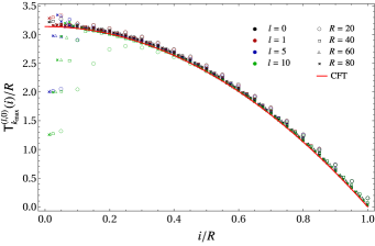
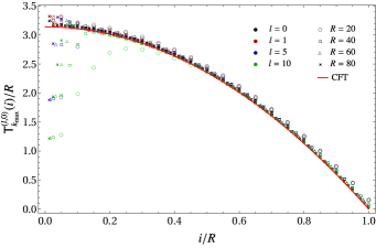
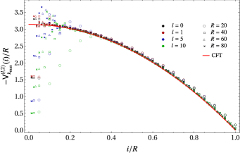
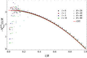
Figure 3: $\mathsf{T}_{k_{\textrm{\tiny max}}}^{(l,0)}/R$ from (3.14) (top panels) and $-\,\mathsf{V}_{k_{\textrm{\tiny max}}}^{(l,2)}/R$ from (3.21) (bottom panels), when $\omega=0$ and either $d=2$ (left panels) or $d=3$ (right panels), for small values of $l$ and $k_{\textrm{\tiny max}}=R/10$ for every $l$ (other choices for $k_{\textrm{\tiny max}}$ have been considered in Fig. 14). The red curve corresponds to the CFT prediction (1.2).

The expansion of (3.11) gives

$$H_{V,\boldsymbol{l}}=\frac{\mathcal{R}}{a^{2}}\int_{0}^{\mathcal{R}}\Bigg{\{}\mathcal{V}_{k_{\textrm{\tiny max}}}^{(l,0)}(r)\,\Phi_{\boldsymbol{l}}(r)^{2}+a\sum_{\eta}\sum_{k=1}^{k_{\textrm{\tiny max}}}\eta k\bigg{[}\,\frac{1}{2}\,\nu_{l,k,\eta}^{\prime}(r)\,\Phi_{\boldsymbol{l}}(r)+\nu_{l,k,\eta}(r)\,\Phi_{\boldsymbol{l}}(r)^{\prime}\,\bigg{]}\Phi_{\boldsymbol{l}}(r)$$

$$\hskip 113.81102pt+\;a^{2}\,\sum_{\eta}\sum_{k=1}^{k_{\textrm{\tiny max}}}\frac{k^{2}}{2}\left[\,\frac{1}{4}\,\nu_{l,k,\eta}^{\prime\prime}(r)\,\Phi_{\boldsymbol{l}}(r)+\partial_{r}\Big{(}\nu_{l,k,\eta}(r)\,\Phi_{\boldsymbol{l}}^{\prime}(r)\Big{)}\,\right]\Phi_{\boldsymbol{l}}(r)\Bigg{\}}\,\textrm{d}r$$

where $O(a)$ terms have been neglected and

$$\mathcal{V}_{k_{\textrm{\tiny max}}}^{(l,0)}(r)\equiv\lim_{R\to\infty}\frac{\mathsf{V}_{k_{\textrm{\tiny max}}}^{(l,0)}(i)}{R}$$ (3.17)

with $\mathsf{V}_{k_{\textrm{\tiny max}}}^{(l,0)}(i)$ being defined as

$$\mathsf{V}_{k_{\textrm{\tiny max}}}^{(l,0)}(i)\,\equiv\,V^{(l)}_{i,i}+\sum_{\eta}\sum_{k=1}^{k_{\textrm{\tiny max}}^{(\eta)}}V^{(l)}_{i,i+\eta k}\,.$$ (3.18)

The numerical results displayed in Fig. 4 indicate that the limit (3.17) provides a well defined finite function when $k_{\textrm{\tiny max}}$ is large enough (see (3.28)), at least for small the values of $l$ that we have considered.

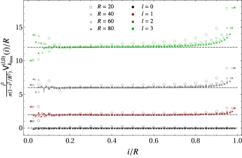
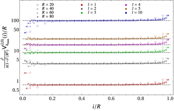
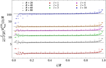
Figure 4: $\mathsf{V}_{k_{\textrm{\tiny max}}}^{(l,0)}/R$ from (3.18) when $\omega=0$ and either $d=2$ (left panels) or $d=3$ (right panels), for small values of $l$ and $k_{\textrm{\tiny max}}=R/10$ for every $l$ (other choices for $k_{\textrm{\tiny max}}$ have been considered in Fig. 15). The horizontal dashed lines correspond to (2.11), i.e. to $l^{2}-1/4$ in the left panels and to $l(l+1)$ in the right panels. In the bottom panels the data corresponding to $1\leqslant l\leqslant 10$ are shown by adopting the logarithmic scale for the vertical axes.

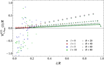
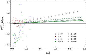
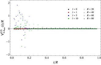
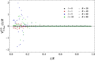
Figure 5: $\mathsf{V}_{1,k_{\textrm{\tiny max}}}^{(l,2)}/R$ (top panels) and $\mathsf{V}_{2,k_{\textrm{\tiny max}}}^{(l,2)}/R$ (bottom panels), from (3.23) and (3.25) respectively, when $\omega=0$ and either $d=2$ (left panels) or $d=3$ (right panels), for various values of $l$ and $R$. Here $k_{\textrm{\tiny max}}=R/10$ for every $l$.

Since the integrand of the $O(1/a)$ term in (3) is proportional to the total derivative $\partial_{r}[\nu_{l,k,\eta}(r)\,\Phi(r)^{2}]$, the corresponding integral gives the boundary terms $[\nu_{l,k,\eta}(r)\,\Phi(r)^{2}]|^{r=\mathcal{R}}_{r=0}\,$. One of these boundary terms vanishes because $\nu_{l,k,\eta}(\mathcal{R})=0$, while the other one does not contribute because of the Dirichlet boundary condition $\Phi_{\boldsymbol{l}}(0)=0$ imposed at the origin. Thus, (3) simplifies to

$$H_{V,\boldsymbol{l}}=\frac{\mathcal{R}}{a^{2}}\int_{0}^{\mathcal{R}}\mathcal{V}_{k_{\textrm{\tiny max}}}^{(l,0)}(r)\,\Phi_{\boldsymbol{l}}(r)^{2}\,\textrm{d}r$$ (3.19)

$$\hskip 8.5359pt+\;\mathcal{R}\int_{0}^{\mathcal{R}}\;\sum_{\eta}\sum_{k=1}^{k_{\textrm{\tiny max}}}\frac{k^{2}}{2}\left[\,\frac{1}{4}\,\nu_{l,k,\eta}^{\prime\prime}(r)\,\Phi_{\boldsymbol{l}}(r)+\nu_{l,k,\eta}^{\prime}(r)\,\Phi_{\boldsymbol{l}}^{\prime}(r)+\nu_{l,k,\eta}(r)\,\Phi_{\boldsymbol{l}}^{\prime\prime}(r)\,\right]\Phi_{\boldsymbol{l}}(r)\,\textrm{d}r\,.$$

The last term of this expression, whose integrand is $\nu_{l,k,\eta}(r)\,\Phi^{\prime\prime}_{\boldsymbol{l}}(r)\,\Phi_{\boldsymbol{l}}(r)$, can be studied by employing (3.5) and introducing

$$\mathcal{V}_{k_{\textrm{\tiny max}}}^{(l,2)}(r)\equiv\lim_{R\to\infty}\frac{\mathsf{V}_{k_{\textrm{\tiny max}}}^{(l,2)}(i)}{R}$$ (3.20)

where

$$\mathsf{V}_{k_{\textrm{\tiny max}}}^{(l,2)}(i)\equiv\sum_{\eta}\sum_{k=1}^{k_{\textrm{\tiny max}}^{(\eta)}}\frac{k^{2}}{2}\,V^{(l)}_{i,i+\eta k}\,.$$ (3.21)

In the bottom panels of Fig. 3 we display numerical results indicating that the limit (3.20) gives a well defined finite function when $k_{\textrm{\tiny max}}$ is large enough (see (3.27)).

As for the term in (3.19) whose integrand is $\nu_{l,k,\eta}^{\prime}(r)\,\Phi_{\boldsymbol{l}}^{\prime}(r)\,\Phi_{\boldsymbol{l}}(r)$, since the analytic expressions for $\nu_{l,k,\eta}(r)$ are not known, we approximate $\nu_{l,k,\eta}^{\prime}(r)$ through finite differences, i.e. by replacing this function with $[\nu_{l,k,\eta}(r+a)-\nu_{l,k,\eta}(r)]/a$. This approximation, combined with (3.5) and (3.19), leads to introduce

$$\mathcal{V}_{1,k_{\textrm{\tiny max}}}^{(l,2)}(r)\equiv\lim_{R\to\infty}\frac{\mathsf{V}_{1,k_{\textrm{\tiny max}}}^{(l,2)}(i)}{R}$$ (3.22)

with $\mathsf{V}_{1,k_{\textrm{\tiny max}}}^{(l,2)}(i)$ being defined as follows

$$\mathsf{V}_{1,k_{\textrm{\tiny max}}}^{(l,2)}(i)\equiv\sum_{\eta}\sum_{k=1}^{k_{\textrm{\tiny max}}^{(\eta)}}\frac{k^{2}}{2}\Big{(}V^{(l)}_{i+1,i+\eta k+1}-V^{(l)}_{i,i+\eta k}\Big{)}\,.$$ (3.23)

Similarly, for the term in (3.19) whose integrand is $\nu^{\prime\prime}_{l,k,\eta}(r)\,\Phi^{2}_{\boldsymbol{l}}(r)$ we approximate $\nu_{l,k,\eta}^{\prime\prime}(r)$ through finite differences. This leads to define

$$\mathcal{V}_{2,k_{\textrm{\tiny max}}}^{(l,2)}(x)\equiv\lim_{R\to\infty}\frac{\mathsf{V}_{2,k_{\textrm{\tiny max}}}^{(l,2)}(i)}{R}$$ (3.24)

with

$$\mathsf{V}_{2,k_{\textrm{\tiny max}}}^{(l,2)}(i)\,\equiv\,\sum_{\eta}\sum_{k=1}^{k_{\textrm{\tiny max}}^{(\eta)}}\frac{k^{2}}{2}\Big{(}V^{(l)}_{i+1,i+\eta k+1}-2\,V^{(l)}_{i,i+\eta k}+V^{(l)}_{i-1,i+\eta k-1}\Big{)}\,.$$ (3.25)

The subindices $1$ and $2$ in the l.h.s.’s of (3.22)-(3.23) and of (3.24)-(3.25) respectively indicate that the corresponding quantities are related to $\nu_{l,k,\eta}^{\prime}(r)$ and $\nu_{l,k,\eta}^{\prime\prime}(r)$. In the top and bottom panels of Fig. 5 we show some numerical results telling us that the limits in (3.22) and (3.24) respectively give the function that vanishes identically (see (3.29)).

Finally, by employing the expressions (3.13), (3.20), (3.22) and (3.24) as discussed above, we take the limit $k_{\textrm{\tiny max}}\to\infty$ in (3.12) and (3.19), finding for the non vanishing contributions the following expression

$$\frac{H_{T,\boldsymbol{l}}+H_{V,\boldsymbol{l}}}{2} = \frac{\mathcal{R}}{a^{2}}\int_{0}^{\mathcal{R}}\frac{1}{2}\left[\,\mathcal{V}_{\infty}^{(l,0)}(r)+\frac{1}{4}\,\mathcal{V}_{2,\infty}^{(l,2)}(r)\right]\Phi_{\boldsymbol{l}}(r)^{2}\,\textrm{d}r\,$$ (3.26)

$$+\,\mathcal{R}\int_{0}^{\mathcal{R}}\frac{1}{2}\,\Big{[}\,\mathcal{T}_{\infty}^{(l,0)}(r)\,\Pi_{\boldsymbol{l}}(r)^{2}+\mathcal{V}_{1,\infty}^{(l,2)}(r)\,\Phi_{\boldsymbol{l}}^{\prime}(r)\,\Phi_{\boldsymbol{l}}(r)+\mathcal{V}_{\infty}^{(l,2)}(r)\,\Phi_{\boldsymbol{l}}^{\prime\prime}(r)\,\Phi_{\boldsymbol{l}}(r)\,\Big{]}\textrm{d}r$$

where it is assumed that the weight functions are well defined. Since the CFT expression (1.1) is valid when $\mathcal{R}_{\textrm{\tiny tot}}\to\infty$, we must consider $R\ll R_{\textrm{\tiny tot}}$ in order to compare our numerical results with this CFT formula specialised to the massless scalar field. The main outcomes of our numerical analysis are shown in Fig. 3, Fig. 4 and Fig. 5, where the data reported in the left panels and in the right panels correspond to $d=2$ and $d=3$ respectively. These results provide some numerical evidence supporting the conjecture that (3.26) provides the CFT prediction (1.1) for the massless scalar field.

In Fig. 3 the combinations of diagonals defined in (3.14) and (3.21) are considered. The numerical data shown in this figure lead us to conjecture that

$$\mathcal{T}_{\infty}^{(l,0)}(r)\,=\,\beta(r)\;\;\;\qquad\;\;\;-\mathcal{V}_{\infty}^{(l,2)}(r)\,=\,\beta(r)$$ (3.27)

where $\beta(r)$ is the parabola (1.2) restricted to $0\leqslant r\leqslant\mathcal{R}$, which is independent both of the dimensionality parameter $d$ and of the mode parameter $l$.

In Fig. 4 we report numerical data points for the combination of diagonals (3.17) which support the following conjecture

$$\frac{\mathcal{V}_{k_{\textrm{\tiny max}}}^{(l,0)}(r)}{a^{2}}\;\longrightarrow\;\mu_{d}(l)\,\frac{\beta(r)}{r^{2}}\,.$$ (3.28)

The horizontal dashed lines in both the panels of Fig. 4 correspond to the coefficient $\mu_{d}(l)$ defined in (2.11). We find it worth highlighting that, although the diagonals shown in Fig. 2 for $d=2$ and $d=3$ seem identical, their combination (3.18) displays the peculiar dependence on $d$ given by (2.11), as shown in Fig. 4. This is a characteristic feature of the fact that we are considering an entanglement Hamiltonian in a Minkowski spacetime with a number of spatial dimensions strictly larger than one; indeed, the term corresponding to (3.28) gives the vanishing function when $d=1$. Near the boundary of the sphere, i.e. where $i/r\sim 1^{-}$, the discrepancy between the data points (which are obtained as a ratio of two quantities that are both vanishing at the boundary of the sphere) and (3.28) increases with $l$. These discrepancies becomes very similar when the logarithmic scale is adopted (see the bottom panels of Fig. 4).

In Fig. 5 we show numerical data for the combinations of diagonals introduced in (3.23) and (3.25). In this case the curves for different sizes $R$ do not collapse and tend to zero as $R$ increases; hence it is natural to conjecture that

$$\mathcal{V}_{1,\infty}^{(l,2)}(r)\,=\,0\;\;\;\qquad\;\;\;\mathcal{V}_{2,\infty}^{(l,2)}(r)\,=\,0\,.$$ (3.29)

We emphasise that large values of $k_{\textrm{\tiny max}}$ are needed to obtain the numerical results described above. In appendix B we show that the expected CFT results are not obtained when $k_{\textrm{\tiny max}}$ is not large enough. This crucial message can be appreciated e.g. for (3.27) and (3.28) by comparing the right panels of Fig. 3 and Fig. 4 with Fig. 14 and Fig. 15 respectively. The conjecture (3.28) naturally leads to ask how $k_{\textrm{\tiny max}}\to\infty$ should be taken in the continuum limit. In Fig. 3, Fig. 4 and Fig. 5 the ratio $k_{\textrm{\tiny max}}/R$ is kept fixed (and equal to $1/10$) as $R$ increases. In the appendix B we report and discuss also numerical results obtained by keeping $k_{\textrm{\tiny max}}$ fixed as $R$ increases (see Fig. 14 and Fig. 15). We find that these two different limiting procedures give the same results for the quantities that we are considering. However, this question deserves further investigations. Notice also that all the data reported in Fig. 3, Fig. 4 and Fig. 5 do not display good collapses around the center of the sphere (i.e. where $i/R\sim 0^{+}$): we expect that larger systems are needed to observe them.

The conjectures (3.27), (3.28) and (3.29) have been formulated for any value of $l$. However, the data points in Fig. 3, Fig. 4 and Fig. 5 provide numerical support to these conjectures only for the small values of $l$ that we have been able to explore. The validity of (3.27), (3.28) and (3.29) for any $l$ is a strong assumption and we find it worth improving the numerical analysis described above in order to check it also for higher values of $l$.

Finally, by inserting (3.27), (3.28) and (3.29) into (3.26), one concludes that (2.17) is the continuum limit of the operator (2.18). Then, the summation (2.16) provides the final CFT result for the entanglement Hamiltonian of the sphere for the massless scalar field.

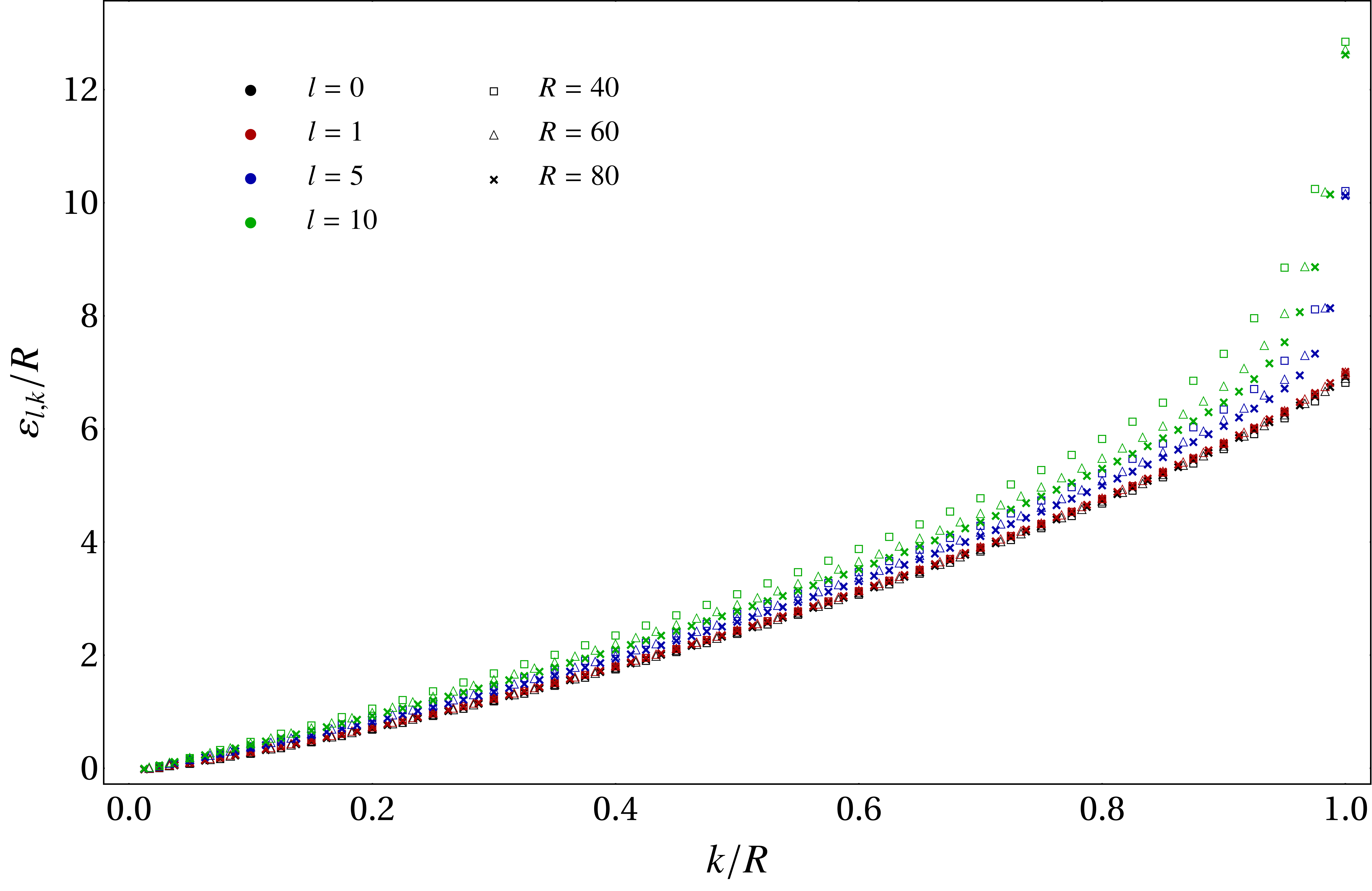
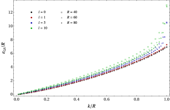
Figure 6: Single particle entanglement energies at given $l$ in the case of $\omega=0$ when $d=2$ (left panel) and $d=3$ (right panel), for various values of $l$ and $R$.

We find worth discussing also some numerical results for the entanglement entropy. Since the ground state is the direct product of the ground states corresponding to $\widehat{H}_{\boldsymbol{l}}$, the entanglement entropy of the sphere $S_{B}$ is obtained by summing the contributions corresponding to all the different values of $\boldsymbol{l}$ [2]. These contributions can be evaluated through the symplectic eigenvalues of the reduced covariance matrix $Q_{l,B}\oplus P_{l,B}$ at given $l$ or, equivalently, through the single particle entanglement energies at given $l$ [37, 33, 50, 34, 51, 52], as briefly anticipated in Sec. 2.2. Since $Q_{l,B}\oplus P_{l,B}$ depends only on $l$, the entanglement entropy of the sphere $B$ is computed as follows [2]

$$S_{B}=\sum_{l=0}^{\infty}N_{d,l}\,S_{B,l}\;\;\;\;\qquad\;\;\;\;S_{B,l}\equiv\sum_{k=1}^{R}\left(\,\frac{\varepsilon_{l,k}}{e^{\varepsilon_{l,k}}\ -1}-\log\!\big{(}1-e^{-\varepsilon_{l,k}}\big{)}\right)$$ (3.30)

which has been explored numerically in various studies [2, 9, 41, 42, 45, 43].

In Fig. 6 we show the single particle entanglement energies $\varepsilon_{l,k}/R$ at given $l$ in terms of $k/R$ when $\omega=0$, for $d=2$ (left panel) and $d=3$ (right panel). The summand in $S_{B,l}$ diverges as $\varepsilon_{l,k}\to 0^{+}$; hence the low-lying part of the single particle entanglement spectrum at fixed $l$ provides the largest contribution to $S_{B,l}$. Clear differences between $\varepsilon_{l,k}/R$ for $d=2$ and $d=3$ are not visible, despite the fact that $Q_{l,B}\oplus P_{l,B}$ depends explicitly on $d$ (see (2.14)).

In the left panel of Fig. 7, we show some numerical data for $S_{B,l}$ defined in (3.30) which display a clear dependence on the dimensionality parameter $d$ for this quantity. In this panel the dashed curve corresponds to $\frac{1}{6}\log(R)+\mathrm{const}$, which is the entanglement entropy of a segment at the beginning of the semi-infinite line [6] and it coincides with $S_{B,0}$ when $d=3$, as expected from the fact that $\mu_{1}(0)=\mu_{3}(0)=0$. Moreover, the data corresponding to $(d,l)=(2,1)$ coincides with ones corresponding to $(d,l)=(4,0)$ because (2.11) gives $3/4$ in both these cases. In the right panel of Fig. 7 we display some numerical results for the entanglement entropy $S_{B}$ (obtained through (3.30) by restricting the sum over $l$ to $l\leqslant 1000$) showing the area law behaviour first observed in [2] in a clear way. The dashed lines in this panel correspond to $\alpha(d)\,R^{d-1}$ and the fitted values of the slopes are $\alpha(2)=0.46$ and $\alpha(3)=0.30$, in agreement with the numerical results reported e.g. in [2, 41, 43].

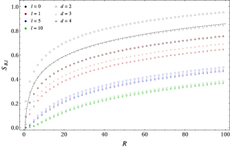
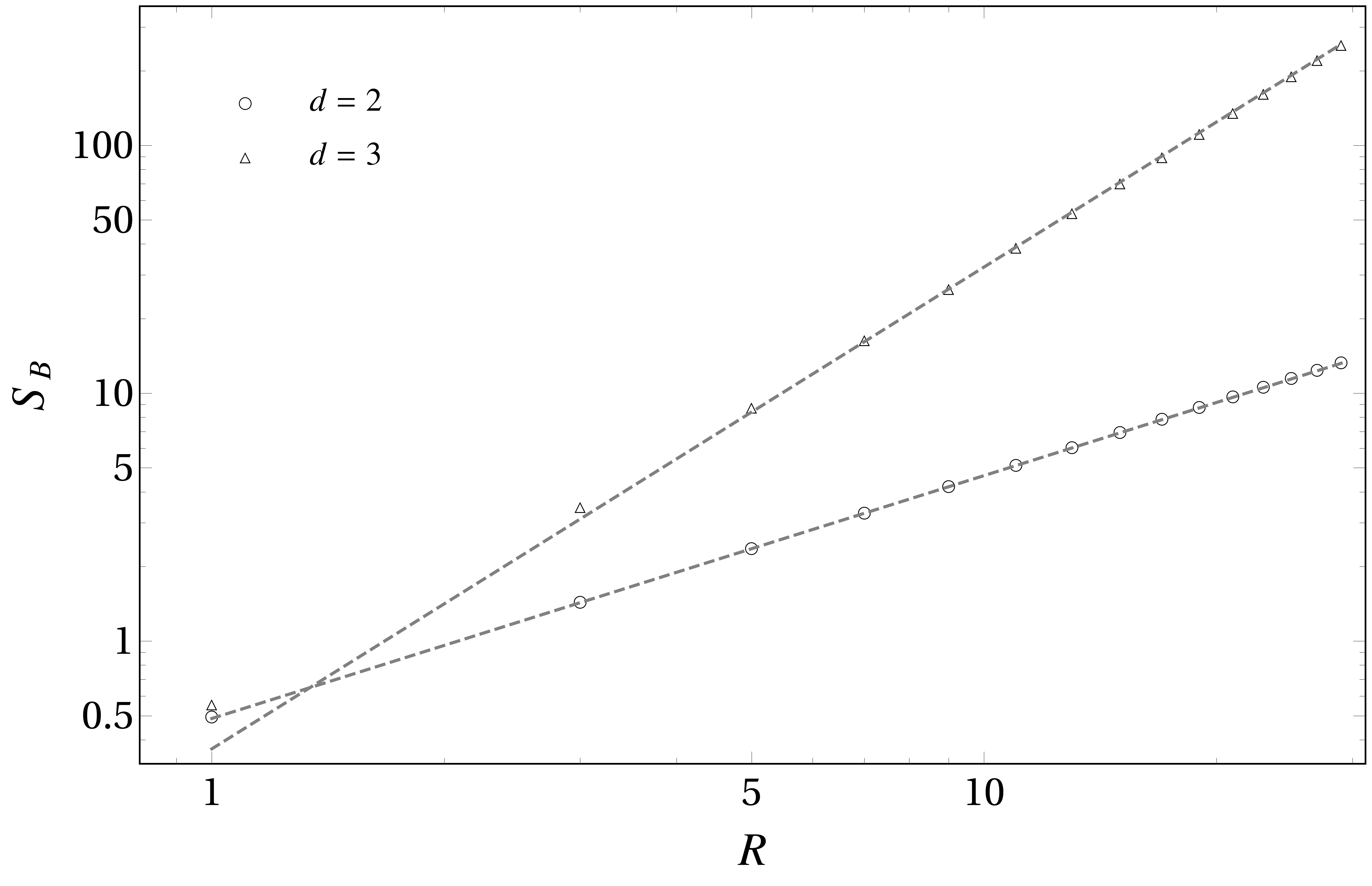
Figure 7: The quantity $S_{B,l}$ (left panel) and the entanglement entropy $S_{B}$ (right panel), defined in (3.30), when $\omega=0$ and for some values of $d$.

Many interesting results have been obtained for the entanglement entropy of the sphere and other interesting subregions in the continuum limit for generic $d$ through various quantum field theory mehods [6, 53, 54, 55, 56, 57, 58, 49, 59]. It would be instructive to explore whether these methods can be employed to study also the corresponding entanglement Hamiltonians.

4 Entanglement Hamiltonian at $\omega>0$

In this section we consider the entanglement Hamiltonian of the $d$ dimensional sphere $B$ in the regularised model of [2] introduced in Sec. 2 when $\omega>0$ and the entire system is in its ground state. We adapt to this case the analysis performed in [26] for the entanglement Hamiltonian of a block made by consecutive sites in the infinite and non-critical harmonic chain. The numerical setup is the one described in Sec. 3 and, since the outcomes for $d=2$ and $d=3$ are very similar, in the following we report only the results corresponding to $d=3$.

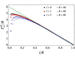
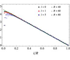
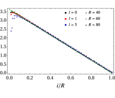
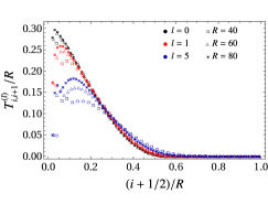
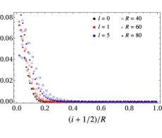
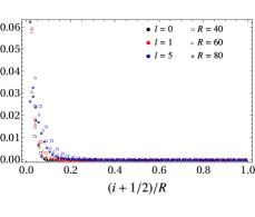
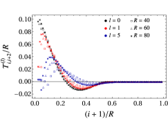
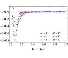
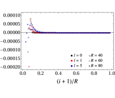
Figure 8: Short-range couplings in the matrices $T^{(l)}/R$ (see (3.2) and (3.5)) when $\omega>0$ and $d=3$, for $\omega=1$ (left panels), $\omega=3$ (middle panels) and $\omega=5$ (right panels), for some small $l$’s and different sizes $R$. The dashed green lines in the top panels correspond to (4.1).

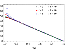
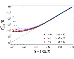
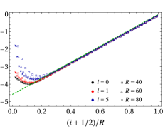
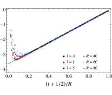
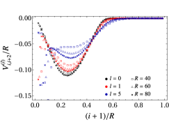
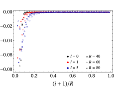
Figure 9: Short-range couplings in the matrices $V^{(l)}/R$ (see (3.2) and (3.5)) when $\omega>0$ and $d=3$, for $\omega=1$ (left panels), $\omega=3$ (middle panels) and $\omega=5$ (right panels), for some $l$’s and different $R$. The dashed green lines in the top and middle panels correspond to (4.2).

In Fig. 8 and Fig. 9 we show the numerical data points for the diagonals of the matrices $T^{(l)}$ and $V^{(l)}$ respectively, evaluated from (2.2) when $d=3$ and for $\omega=1$ (left panels), $\omega=3$ (central panels) or $\omega=5$ (right panels). It is instructive to compare these results against the corresponding ones obtained for $\omega=0$ and displayed in Fig. 1 and Fig. 2. Also for $\omega>0$, data collapses are observed for small values of $l$. Presumably, larger systems are needed to observe these collapses also for higher values of $l$.

The considerations made in [26] for the entanglement Hamiltonian of a block of consecutive sites in the infinite and non-critical harmonic chain can be adapted to this case in a straightforward way, with the crucial difference that only one point separates the subsystem from its complementary region along the radial direction of the sphere $B$. When $\omega>0$ and $l$ are fixed, for all the diagonals $T^{(l)}_{i,i+k}$ and $V^{(l)}_{i,i+k}$ with $k\geqslant 0$ except for $T^{(l)}_{i,i}$, $V^{(l)}_{i,i}$ and $V^{(l)}_{i,i+1}$ we can identify a region closed to the boundary of the sphere where the diagonal vanishes. For a given $l$, the size of this region increases with $k$ at fixed $\omega$ and it also increases with $\omega$ at a given $k$. Thus, in the large mass regime only the three diagonals $T^{(l)}_{i,i}$, $V^{(l)}_{i,i}$ and $V^{(l)}_{i,i+1}$ are non vanishing. Furthermore, when $\omega\gg l$ and for the small values of $l$ considered, we find that the analytic results found in [26] (which are based on [27]) can be easily adapted to the case of the sphere. In particular, the dominant matrix elements are well approximated by

$$\frac{T^{(l)}_{i,i}}{R}\,=\,2b(\kappa)\,\big{(}1-i/R\big{)}$$ (4.1)

and

$$\frac{V^{(l)}_{i,i}}{R}\,=\,\big{(}\omega^{2}+2\big{)}\,2b(\kappa)\,\big{(}1-i/R\big{)}\;\;\;\qquad\;\;\;\frac{V^{(l)}_{i,i+1}}{R}\,=\,-\,2b(\kappa)\,\big{(}1-i/R\big{)}$$ (4.2)

where

$$b(\kappa)\,\equiv\,2\,I(\tilde{\kappa})\,\sqrt{\kappa}$$ (4.3)

with $I(\kappa)$ being the complete elliptic integral of the first kind and

$$\kappa\,\equiv\,\frac{1}{4}\Big{(}\sqrt{\omega^{2}+4}-\omega\Big{)}^{2}\;\;\;\qquad\;\;\;\tilde{\kappa}\equiv\sqrt{1-\kappa^{2}}\,.$$ (4.5)

The analytic results in (4.1) and (4.2) correspond to the straight green dashed lines in Fig. 8 and in Fig. 9 respectively. The massive scalar field in the continuum limit is described by taking $\omega\to 0$ and $a\to 0$ while $\omega/a$ is kept fixed. When $\omega\to 0$, we have that $\kappa\to 1$ and $\tilde{\kappa}\to 0$; hence $I(\tilde{\kappa})\to\pi/2$ and therefore $2b(\kappa)\to 2\pi$, which is the value predicted by Bisognano and Wichmann [10, 11], as already remarked in [26]. Notice that the analytic expressions in (4.1) and (4.2) are independent both of $d$ and of $l$. Our numerical results for $d=2$ and $d=3$ confirm this observation (in this section we show only the data corresponding to $d=3$). In Fig. 8 and in Fig. 9 one observes a dependence on the angular momentum parameter $l$ only in the central region of the sphere, where the numerical data do not follow the straight lines given by (4.1) and (4.2).

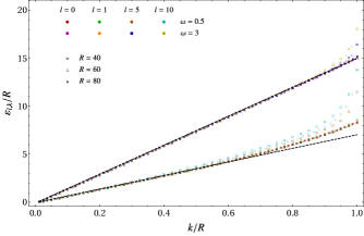
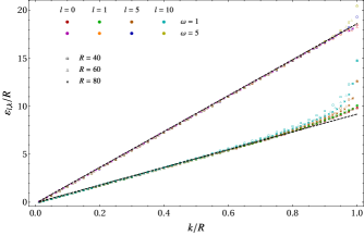
Figure 10: Single particle entanglement energies at fixed $l$ for $d=3$ and $\omega\in\{0.5\,,1\,,3\,,5\}$. The dashed lines correspond to (4.6).

The symplectic spectrum of the reduced covariance matrix $Q_{l,B}\oplus P_{l,B}$ at a given $l$ provides the corresponding single particle entanglement energies $\varepsilon_{l,k}$ at fixed $l$ as discussed in Sec. 2.2. In Fig. 10 we show numerical data for $\varepsilon_{l,k}$ (in the case of $d=3$) when $l$ is small for some values of $\omega$. By comparing these results with the corresponding ones for $\omega=0$ displayed in Fig. 6, we observe that $\varepsilon_{l,k}$ as function of $k/R$ are well described by a straight line as $\omega$ increases. This feature has been already highlighted for $d=1$ in the case of the block of consecutive sites in the infinite harmonic chain on the line [26]. Furthermore, the slope of this straight line is given by the same expression found in [26] for the $d=1$ case, namely [28]

$$\varepsilon_{l,k}=(2k-1)\,\varepsilon\;\;\;\qquad\;\;\;\varepsilon\equiv\pi\,\frac{I(\tilde{\kappa})}{I(\kappa)}$$ (4.6)

where $\kappa$ and $\tilde{\kappa}$ have been defined in (4.5).

Numerical results for the entanglement entropy $S_{B}$ of the sphere when $\omega>0$ are shown in the right panel of Fig. 11 (see the right panel of Fig. 7 for $S_{B}$ when $\omega=0$). They have been obtained through (3.30), with the sum over $l$ restricted to $l\leqslant 500$ for $\omega=1$ and $\omega=3$, and to $l\leqslant 1000$ for $\omega=5$. The dashed lines correspond to $\alpha(d,\omega)\,R^{d-1}$ for some fitted values of the constants $\alpha(d,\omega)$; hence these data just highlight the expected area law behaviour of the entanglement entropy.

Similarly to the massless case, also when $\omega>0$ the dependence on $d$ and $l$ is more visible in the quantity $S_{B,l}$ defined in (3.30). In the left panel of Fig. 11 we show $S_{B,l}$ in terms of $R$ for $\omega=1$ and $\omega=3$, finding a qualitatively different behaviour with respect to the massless case (see the left panel of Fig. 7). In particular, the horizontal dashed line providing the asymptotic value of $S_{B,l}$ in the left panel of Fig. 11 is given by [8, 26]

$$S_{0}\equiv-\frac{1}{24}\left[\,\log\!\left(\frac{16\,\tilde{\kappa}^{4}}{\kappa^{2}}\right)-(1+\kappa^{2})\,\frac{4\,I(\kappa)I(\tilde{\kappa})}{\pi}\,\right].$$ (4.7)

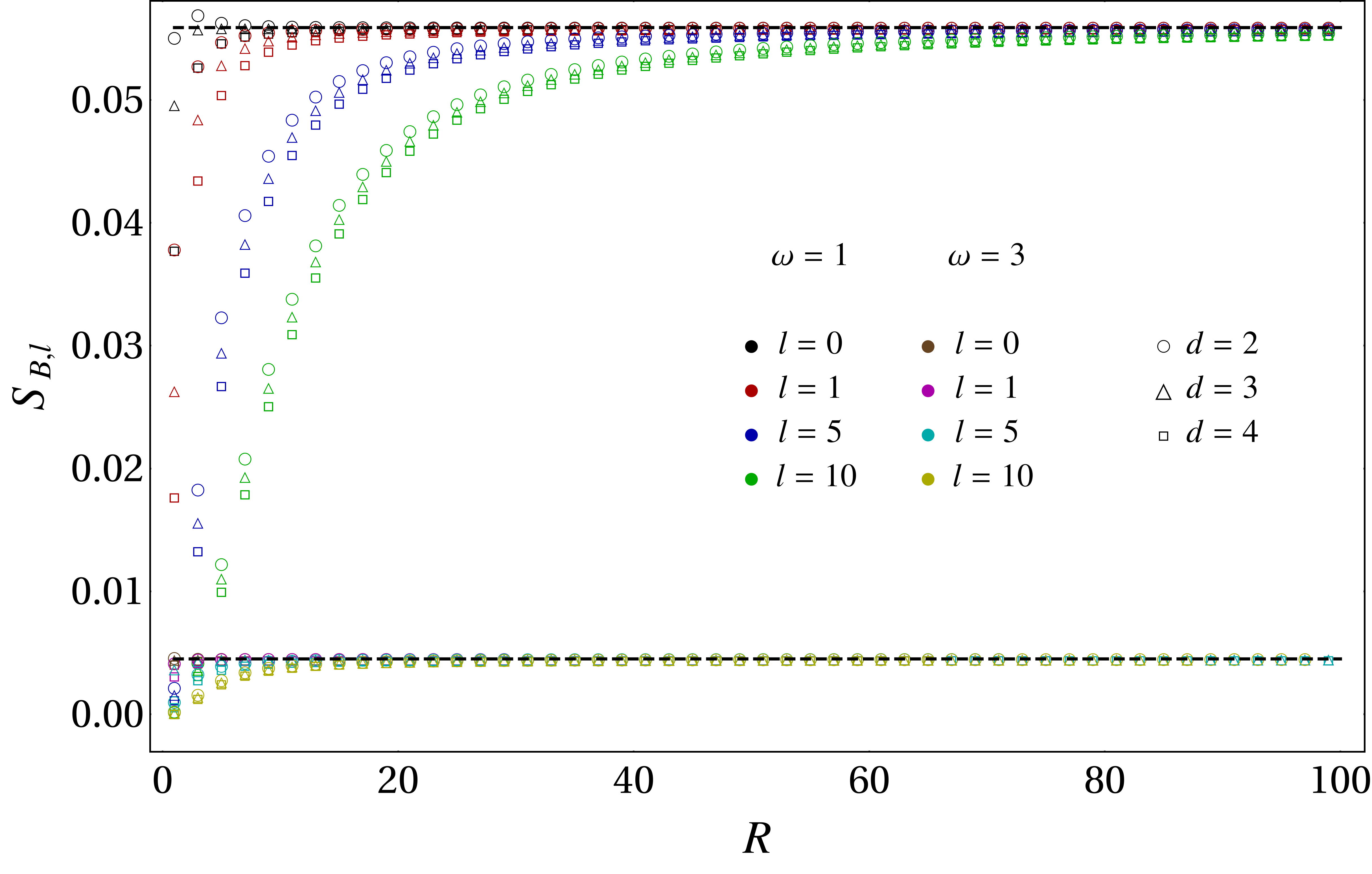
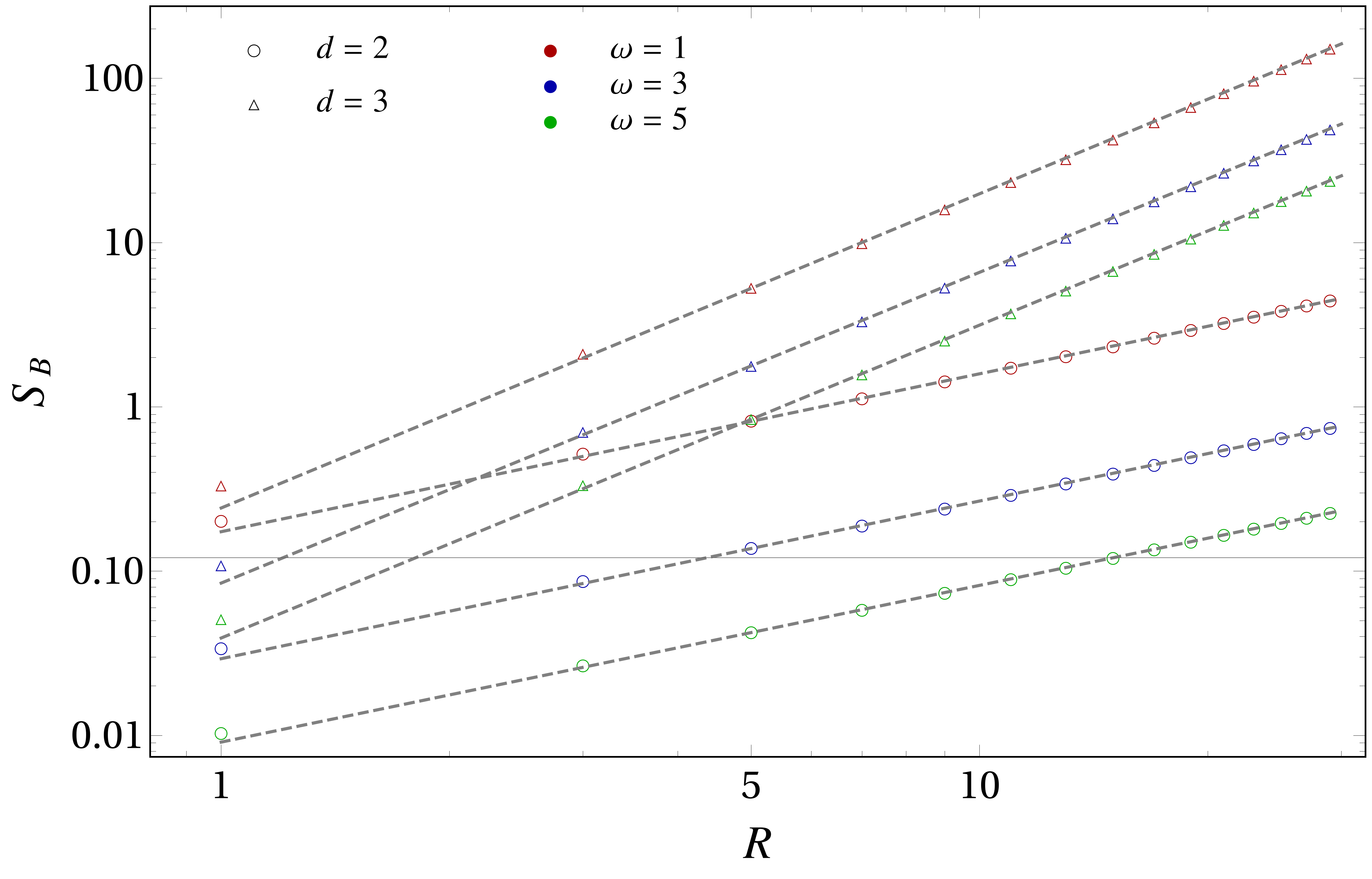
Figure 11: The entanglement entropy $S_{B}$ (right panel) and $S_{B,l}$ (left panel) defined in (3.30) when $\omega>0$. The horizontal dashed lines in the left panel correspond to (4.7).

We remark that the above numerical analysis does not correspond to the continuum limit of the entanglement Hamiltonian for the massive scalar field, where $\omega\to 0$ and $R\to\infty$ while $\omega R$ is kept fixed. In this regime we have encountered the same difficulties discussed in [26] for the entanglement Hamiltonians of a block of consecutive sites in non-critical free chains on the infinite line.

5 Conclusions

We have explored the continuum limit of the entanglement Hamiltonian of a sphere in the $d+1$ dimensional Minkowski spacetime for a massless scalar field. We have employed a numerical analysis based on the radial lattice discretisation introduced in [2], on the results found in [2, 9] and on the procedure already introduced [21, 22, 24, 25, 23] to study some entanglement Hamiltonians of a block of consecutive sites in one-dimensional free chains. Our main results for the massless scalar field are the conjectures given by (3.27), (3.28) and (3.29), which are supported by the numerical data reported in Fig. 3, Fig. 4 and Fig. 5 in the cases of $d=2$ and $d=3$ and for small values of the total angular momentum parameter $l$. By employing these conjectured results into (3.26), we have obtained the expression (2.17) in the continuum, which can be derived also from the entanglement Hamiltonian of the sphere for a generic CFT in its ground state [12, 13] (see (1.1)) specialised to the massless scalar field. An explicit dependence on the dimensionality parameter $d$ and on the total angular momentum parameter $l$ occurs in the term (3.28), which vanishes identically when $d=1$. In the special case of $d=1$, we recover the results of [25] for the entanglement Hamiltonian of an interval at the beginning of the semi-infinite line with Dirichlet boundary conditions at the origin.

As for the massive regime, we have discussed numerical results obtained for a given $\omega>0$ (see Sec. 4). At a generic value of $\omega\geqslant 0$, the matrix (2.2) characterising the quadratic entanglement Hamiltonian contains long-range and inhomogeneous couplings (see Fig. 8 and Fig. 9). However, in the limit of $\omega\gg l$, only the nearest neighbour couplings are non vanishing and the corresponding weight function along the radial direction is well approximated by straight lines whose slopes are independent of $d$ and $l$ and can be determined analytically (see (4.1) and (4.2)), as already observed in [26] also for the entanglement Hamiltonian of a block of consecutive sites in the harmonic chain on the infinite line and in its ground state.

Our analysis can be improved in various directions. All the numerical checks performed in this manuscript correspond to small values of the total angular momentum parameter $l$; hence an improved numerical analysis is required to explore also the sectors corresponding to higher values of $l$. For the massless scalar, the existence of the functions $\tau_{l,\eta k}$ and $\nu_{l,\eta k}$ introduced in (3.5) is a crucial assumption throughout the derivation of (3.26). It would be interesting to obtain numerical data that support further these conjectures and also to find analytic expressions for these functions, as done in [22] for the entanglement Hamiltonian of a block of consecutive sites in the chain of free fermions on the line. For the massive scalar, it is important to explore through these numerical methods the regime characterised by a given value of $\omega R$ when $R\to\infty$, where the entanglement Hamiltonian of the sphere in the continuum is fully non-local [21, 60].

It would be interesting to employ the procedure discussed in [21, 22, 23, 24, 25, 26] and throughout this manuscript to study the continuum limit of entanglement Hamiltonians where either multi-local [61, 62, 63, 64, 65, 66, 67] or fully non-local terms [68, 60] occur, in systems characterised by spatially inhomogeneity [17] and in systems driven out of equilibrium [16, 69, 70]. It would be insightful also to identify possible boundary terms in the entanglement Hamiltonians [49, 71, 59] through numerical analyses on the lattice.

It is interesting also to develop methods to write lattice operators including only nearest neighbour couplings that approximate the entanglement Hamiltonians [19, 72, 22, 24, 17, 73, 74, 75] and to understand their relation with the corresponding entanglement Hamiltonian, as done e.g. in [19, 22]. A numerical approach to some entanglement Hamiltonains based on a quantum Monte Carlo method has been proposed in [76].

In a generic number of spatial dimensions, we find it worth exploring further also the relations between the entanglement Hamiltonians and other insightful entanglement quantifiers like the entanglement spectrum [77, 78, 16, 73, 17, 79, 70, 80, 81, 82], the contour functions for the entanglement entropies [83, 84, 85] and the logarithmic negativity [86, 87, 88, 36, 89, 90, 91, 92, 93, 94] or other related quantities like the circuit complexity of mixed states [95, 96].

Acknowledgments

We are grateful to Filiberto Ares, Giuseppe Di Giulio, Viktor Eisler, Giuseppe Mussardo, Ingo Peschel, Diego Pontello, Benjamin Walter and in particular to Marina Huerta and Mihail Mintchev for helpful discussions or correspondence. ET’s research has been conducted within the framework of the Trieste Institute for Theoretical Quantum Technologies (TQT).

Appendix A Correlators in the continuum

In this appendix we report the two-point functions in the continuum computed through quantum field theory methods [38, 39] and compare them with the correlators on the lattice (2.15) obtained for different discretizations of the Hamiltonian of the scalar field.

In the spherical coordinates introduced in Sec. 2.1, the two-point function of the free massive scalar field $\Phi(t,r,\Omega)$ in the $d+1$ dimensional Minkowski spacetime reads [39]

$$\langle\,\Phi(t_{1},r_{1},\Omega_{1})\,\Phi(t_{2},r_{2},\Omega_{2})\,\rangle\,=\,\frac{1}{(r_{1}r_{2})^{\frac{d-1}{2}}}\sum_{l=0}^{\infty}\frac{2l+d-2}{(d-2)\,\mathcal{S}_{d}}\;C_{l}^{\frac{d-2}{2}}\!(\cos\xi)\;\mathcal{G}_{l}(t_{1},r_{1};t_{2},r_{2})$$ (A.1)

where $\mathcal{S}_{d}\equiv\tfrac{2\pi^{d/2}}{\Gamma(d/2)}$ is the area of the $d-1$ dimensional unit sphere and

$$\mathcal{G}_{l}(t_{1},r_{1};t_{2},r_{2})\,\equiv\,\frac{\sqrt{r_{1}r_{2}}}{2}\int_{0}^{\infty}\!\!\frac{\gamma}{\sqrt{\gamma^{2}+m^{2}}}\;J_{\tilde{\mu}}(\gamma r_{1})\,J_{\tilde{\mu}}(\gamma r_{2})\;e^{\textrm{i}\sqrt{\gamma^{2}+m^{2}}\,(t_{2}-t_{1})}\,\textrm{d}\gamma$$ (A.2)

with

$$\tilde{\mu}\equiv\sqrt{\frac{1}{4}+\mu_{d}(l)}\,=\,l+\frac{d-2}{2}\,.$$ (A.3)

In (A.1) the angle between directions identified by $\Omega_{1}$ and $\Omega_{2}$ is denoted by $\xi$ and $C_{p}^{q}(x)$ is the Gegenbauer polynomial of degree $p$ and order $q$, which can be expressed also through the hypergeometric function as follows (see e.g. section 15.4 in [30])

$$C_{p}^{q}(x)=\frac{(2q)_{p}}{p!}\;_{2}F_{1}\bigg{(}\!\!-\!p,2q+p\,;q+\frac{1}{2}\,;\frac{1-x}{2}\bigg{)}$$ (A.4)

where $(a)_{b}$ is the Pochhammer symbol.

It is instructive to consider the special case of $d=2$, which is the lowest value of $d$ where the sum over $l$ in (A.1) is non trivial. Taking the limit $d\to 2$ in the infinite sum obtained by isolating the $l=0$ term in (A.1) and using that $\tilde{\mu}=l$ when $d=2$ (from (A.3)), one finds

$$\langle\Phi(t_{1},r_{1},\phi_{1})\,\Phi(t_{2},r_{2},\phi_{2})\rangle=\frac{1}{2\pi\sqrt{r_{1}r_{2}}}\;\bigg{\{}\mathcal{G}_{0}(t_{1},r_{1};t_{2},r_{2})+2\sum_{l\geqslant 1}\cos\!\big{(}l[\phi_{2}-\phi_{1}]\big{)}\,\mathcal{G}_{l}(t_{1},r_{1};t_{2},r_{2})\bigg{\}}\,.$$ (A.5)

For a generic value of $d$, when $t_{1}=t_{2}$ we have that (A.2) simplifies to

$$\mathcal{Q}_{l}(r_{1},r_{2})\,=\,\frac{\sqrt{r_{1}r_{2}}}{2}\int_{0}^{\infty}\!\frac{\gamma}{\sqrt{\gamma^{2}+m^{2}}}\;J_{\tilde{\mu}}(\gamma r_{1})\,J_{\tilde{\mu}}(\gamma r_{2})\,\textrm{d}\gamma\,.$$ (A.6)

When $m=0$ and for $r_{1}<r_{2}$ (which leads to introduce $\rho_{12}\equiv r_{1}/r_{2}<1$), this integral reads

$$\mathcal{Q}_{l}(r_{1},r_{2})\,=\,\frac{\Gamma(\tfrac{1}{2}+\tilde{\mu})}{2\,\Gamma(\tfrac{1}{2})\;\Gamma(1+\tilde{\mu})}\;\rho_{12}^{\tilde{\mu}+1/2}\,{}_{2}F_{1}\!\left(\frac{1}{2}\,,\frac{1}{2}+\tilde{\mu}\,;1+\tilde{\mu}\,;\rho_{12}^{2}\right)$$ (A.7)

which holds for $d\geqslant 2$; indeed, for $d=1$ and $l=0$ we have $\tilde{\mu}=-1/2$, where this expression is not well defined. From (A.2) we can compute also $\partial_{t_{1}}\partial_{t_{2}}\mathcal{G}_{l}(t_{1},r_{1};t_{2},r_{2})$ for $t_{1}=t_{2}$ and the result is

$$\mathcal{P}_{l}(r_{1},r_{2})\,=\,\frac{\sqrt{r_{1}r_{2}}}{2}\int_{0}^{\infty}\!\gamma\,\sqrt{\gamma^{2}+m^{2}}\;J_{\tilde{\mu}}(\gamma r_{1})\,J_{\tilde{\mu}}(\gamma r_{2})\,\textrm{d}\gamma\,.$$ (A.8)

In the massless regime, this becomes

$$\mathcal{P}_{l}(r_{1},r_{2})\,=\,\frac{\Gamma(\frac{3}{2}+\tilde{\mu})\,\rho_{12}^{\tilde{\mu}+\frac{1}{2}}}{\Gamma(\frac{1}{2})\,\Gamma(1+\tilde{\mu})\,(r_{2}^{2}-r_{1}^{2})}\;\Bigg{\{}2\big{[}\,\tilde{\mu}-\rho_{12}^{2}(1+\tilde{\mu})\,\big{]}\;_{2}F_{1}\!\left(\frac{1}{2},\frac{3}{2}+\tilde{\mu}\,;1+\tilde{\mu}\,;\rho_{12}^{2}\right)\hskip 14.22636pt$$

$$\hskip 190.63338pt-\,(1+2\tilde{\mu})\;_{2}F_{1}\!\left(-\frac{1}{2},\frac{3}{2}+\tilde{\mu}\,;1+\tilde{\mu}\,;\rho_{12}^{2}\right)\Bigg{\}}\,.$$

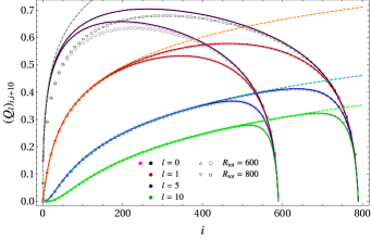
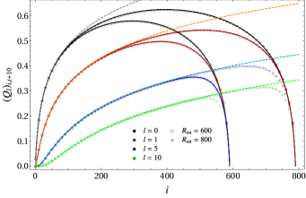
Figure 12: Correlators (2.15) in the massless regime: $Q_{i,i+10}$ (top panels) and $Q_{i,i+100}$ (bottom panels) for $d=2$ (left panels) and $d=3$ (right panels) evaluated from (2.14) with $\omega=0$ and for systems whose total size is given by $R_{\textrm{\tiny tot}}\in\{600,800\}$. The dashed lines correspond to (A.7) and the solid ones to (A.11) with $m=0$. The magenta data points in the left panels are obtained from (A.16) with $\omega=0$.

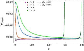
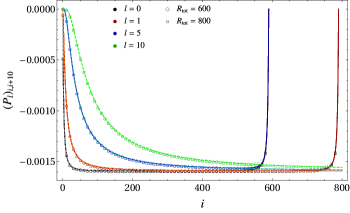
Figure 13: Correlators (2.15) in the massless regime: $P_{i,i+10}$ (top panels) and $P_{i,i+100}$ (bottom panels) for $d=2$ (left panels) and $d=3$ (right panels) evaluated from (2.14) with $\omega=0$ and for systems whose total size is given by $R_{\textrm{\tiny tot}}\in\{600,800\}$. The dashed lines correspond to (A) and the solid ones to (A.12) with $m=0$. The magenta data points are obtained from (A.16) with $\omega=0$.

When the free massive scalar field is defined inside a $d$ dimensional sphere whose radius is $\mathcal{R}_{\textrm{\tiny tot}}$ and Dirichlet boundary conditions are imposed, the two-point function is (A.1) with [39]

$$\mathcal{G}_{l}(t_{1},r_{1};t_{2},r_{2}) \equiv$$ (A.10)

$$\equiv\frac{\sqrt{r_{1}r_{2}}}{2\,\mathcal{R}_{\textrm{\tiny tot}}^{2}}\,\Bigg{[}\,\int_{0}^{\infty}\!\!\frac{\gamma}{\sqrt{(\gamma/\mathcal{R}_{\textrm{\tiny tot}})^{2}+m^{2}}}\;J_{\tilde{\mu}}(\gamma r_{1}/\mathcal{R}_{\textrm{\tiny tot}})\,J_{\tilde{\mu}}(\gamma r_{2}/\mathcal{R}_{\textrm{\tiny tot}})\;e^{\textrm{i}\sqrt{(\gamma/\mathcal{R}_{\textrm{\tiny tot}})^{2}+m^{2}}\,(t_{2}-t_{1})}\,\textrm{d}\gamma$$

$$-\,\frac{2}{\pi}\int_{mR_{\textrm{\tiny tot}}}^{\infty}\frac{K_{\tilde{\mu}}(\gamma)}{I_{\tilde{\mu}}(\gamma)}\;\frac{I_{\tilde{\mu}}(\gamma r_{1}/\mathcal{R}_{\textrm{\tiny tot}})\,I_{\tilde{\mu}}(\gamma r_{2}/\mathcal{R}_{\textrm{\tiny tot}})}{\sqrt{(\gamma/\mathcal{R}_{\textrm{\tiny tot}})^{2}-m^{2}}}\;\gamma\,\cosh\!\big{[}\sqrt{(\gamma/\mathcal{R}_{\textrm{\tiny tot}})^{2}-m^{2}}\,(t_{2}-t_{1})\big{]}\,\textrm{d}\gamma\,\Bigg{]}$$

which simplifies to (A.2) when $\mathcal{R}_{\textrm{\tiny tot}}\to+\infty$, as expected. Setting $t_{1}=t_{2}$ in (A.10), one obtains

$$\mathcal{Q}_{l}(r_{1},r_{2}) \equiv \frac{\sqrt{r_{1}r_{2}}}{2\,\mathcal{R}_{\textrm{\tiny tot}}^{2}}\,\Bigg{[}\,\int_{0}^{\infty}\!\!\frac{\gamma}{\sqrt{(\gamma/\mathcal{R}_{\textrm{\tiny tot}})^{2}+m^{2}}}\;J_{\tilde{\mu}}(\gamma r_{1}/\mathcal{R}_{\textrm{\tiny tot}})\,J_{\tilde{\mu}}(\gamma r_{2}/\mathcal{R}_{\textrm{\tiny tot}})\,\textrm{d}\gamma$$ (A.11)

$$\hskip 56.9055pt-\,\frac{2}{\pi}\int_{m\mathcal{R}_{\textrm{\tiny tot}}}^{\infty}\frac{K_{\tilde{\mu}}(\gamma)}{I_{\tilde{\mu}}(\gamma)}\;\frac{I_{\tilde{\mu}}(\gamma r_{1}/\mathcal{R}_{\textrm{\tiny tot}})\,I_{\tilde{\mu}}(\gamma r_{2}/\mathcal{R}_{\textrm{\tiny tot}})}{\sqrt{(\gamma/\mathcal{R}_{\textrm{\tiny tot}})^{2}-m^{2}}}\;\gamma\,\textrm{d}\gamma\,\Bigg{]}\,.$$

In this finite volume case, we can evaluate $\partial_{t_{1}}\partial_{t_{2}}\mathcal{G}_{l}(t_{1},r_{1};t_{2},r_{2})$ for $t_{1}=t_{2}$ from (A.10), finding

$$\mathcal{P}_{l}(r_{1},r_{2})\,\equiv\,\frac{\sqrt{r_{1}r_{2}}}{2\,\mathcal{R}^{2}_{\textrm{\tiny tot}}}\,\Bigg{[}\,\int_{0}^{\infty}\!\!\gamma\,\sqrt{(\gamma/\mathcal{R}_{\textrm{\tiny tot}})^{2}+m^{2}}\;J_{\tilde{\mu}}(\gamma r_{1}/\mathcal{R}_{\textrm{\tiny tot}})\,J_{\tilde{\mu}}(\gamma r_{2}/\mathcal{R}_{\textrm{\tiny tot}})\,\textrm{d}\gamma$$ (A.12)

$$\hskip 93.89418pt+\,\frac{2}{\pi}\int_{m\mathcal{R}_{\textrm{\tiny tot}}}^{\infty}\!\!\!\sqrt{(\gamma/\mathcal{R}_{\textrm{\tiny tot}})^{2}-m^{2}}\;\frac{K_{\tilde{\mu}}(\gamma)}{I_{\tilde{\mu}}(\gamma)}\;I_{\tilde{\mu}}(\gamma r_{1}/\mathcal{R}_{\textrm{\tiny tot}})\,I_{\tilde{\mu}}(\gamma r_{2}/\mathcal{R}_{\textrm{\tiny tot}})\;\gamma\,\textrm{d}\gamma\,\Bigg{]}\,.$$

In Fig. 12 and Fig. 13 we compare the numerical data points obtained for the correlation matrices given by (2.15) and (2.14) with the corresponding expressions in the continuum, which are given by (A.7) and (A) for the infinite volume regime (dashed lines) and by (A.11) and (A.12) for the finite volume space enclosed in a sphere of radius $\mathcal{R}_{\textrm{\tiny tot}}$ where Dirichlet boundary conditions are imposed on the boundary of the sphere (solid lines). The solid lines that are missing in these figures correspond to the cases where our numerical integration of (A.11) and (A.12) failed. A remarkable agreement between the numerical data points for the lattice correlators and the curves in the continuum is observed, except when $d=2$ and $l=0$ (see the black data points in the left panels of Fig. 12 and Fig. 13).

In order to explain this discrepancy for $(d,l)=(2,0)$, consider $\Delta=\tfrac{1}{r^{d-1}}\,\partial_{r}(r^{d-1}\partial_{r})+\tfrac{1}{r^{2}}\,\tilde{\Delta}$ in (2.1). By employing the decomposition (2.5) first and then performing an integration by parts in the remaining radial integration, one obtains (2.9) with [2, 40, 42, 47, 48]

$$\widetilde{T}_{tt}^{(\boldsymbol{l})} \equiv \frac{1}{2}\,\bigg{\{}\,\Pi_{\boldsymbol{l}}^{2}+r^{d-1}\left[\,\partial_{r}\!\left(\,\frac{\Phi_{\boldsymbol{l}}}{r^{\frac{d-1}{2}}}\right)\right]^{2}+\left(\!-\frac{\lambda_{d}(l)}{r^{2}}+m^{2}\right)\Phi_{\boldsymbol{l}}^{2}\,\bigg{\}}$$ (A.13)

$$= \frac{1}{2}\,\bigg{\{}\,\Pi_{\boldsymbol{l}}^{2}+\big{(}\partial_{r}\Phi_{\boldsymbol{l}}\big{)}^{2}-\frac{d-1}{r}\;\Phi_{\boldsymbol{l}}\,\partial_{r}\Phi_{\boldsymbol{l}}+\frac{(d-1)^{2}}{4\,r^{2}}\;\Phi_{\boldsymbol{l}}^{2}+\left(\!-\frac{\lambda_{d}(l)}{r^{2}}+m^{2}\right)\Phi_{\boldsymbol{l}}^{2}\,\bigg{\}}\hskip 28.45274pt$$ (A.14)

where $\lambda_{d}(l)$ has been defined in (2.3). Notice that, by integrating (A.14) in the radial variable first and then performing an integration by parts in the terms corresponding to $(\partial_{r}\Phi_{\boldsymbol{l}})^{2}$ and $\Phi_{\boldsymbol{l}}\,\partial_{r}\Phi_{\boldsymbol{l}}$, the integral of (2.9) is recovered.

Plugging (A.13) into (2.9), we obtain $H_{\boldsymbol{l}}$. Then, following the regularisation procedure discussed in Sec. 2.1, we find that the corresponding operator in the lattice model along the radial direction reads

$$\widehat{H}_{\boldsymbol{l}}\,=\,\frac{1}{2a}\,\sum_{j=1}^{R_{\textrm{\tiny tot}}}\Bigg{\{}\,\hat{p}_{\boldsymbol{l},j}^{2}+\left(j+\frac{1}{2}\right)^{d-1}\Bigg{[}\,\frac{\hat{q}_{\boldsymbol{l},j+1}}{(j+1)^{\frac{d-1}{2}}}-\frac{\hat{q}_{\boldsymbol{l},j}}{j^{\frac{d-1}{2}}}\,\Bigg{]}^{2}+\left(\!-\frac{\lambda_{d}(l)}{r^{2}}+m^{2}\right)\hat{q}_{\boldsymbol{l},j}^{2}\,\Bigg{\}}$$ (A.15)

which can be written in the form (2.13) with

$$(M_{l})_{j,j}\,\equiv\,-\frac{\lambda_{d}(l)}{j^{2}}+m^{2}+\mathcal{M}_{j}\;\;\qquad\;\;(M_{l})_{j,j+1}\,\equiv\,-\left(\frac{j+1/2}{\sqrt{j(j+1)}}\right)^{d-1}$$ (A.16)

where $\mathcal{M}_{j}$ is defined as

$$\mathcal{M}_{1}\equiv\left(\frac{3}{2}\right)^{d-1}\;\;\qquad\;\;\mathcal{M}_{j}\equiv\left(1+\frac{1}{2j}\right)^{d-1}\!\!+\left(1-\frac{1}{2j}\right)^{d-1}\qquad 2\leqslant j\leqslant R_{\textrm{\tiny tot}}\,.$$ (A.17)

The correlation matrices corresponding to (A.15) are (2.15) with $M_{l}$ given by (A.16). For $\omega=0$, we checked that the data points for these correlators perfectly agree with the ones coming from (2.14) and (2.15) reported in Fig. 12 and Fig. 13, except for $(d,l)=(2,0)$. In this case they correspond to the magenta data points in the left panels of Fig. 12 and Fig. 13, which are nicely reproduced by the curves obtained from (A.11) and (A.12) respectively with $m=0$ and $\tilde{\mu}=0$. In massive regime, we have considered e.g. the case of $(d,l)=(2,1)$ and checked numerically that the matrix correlator $Q_{i,i+10}$ evaluated from (2.14) and (2.15) agrees with (A.11) for $\omega=m=0.1$.

Appendix B Comments on the role of $k_{\textrm{\tiny max}}$

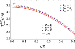
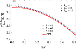
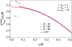
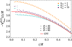
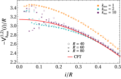
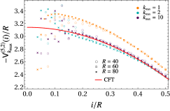
Figure 14: Combinations (3.14) and (3.21) when $\omega=0$ in the case of $d=3$, for various $k_{\textrm{\tiny{max}}}$. These panels should be compared with the right panels of Fig. 3.

In this appendix we briefly discuss the role of $k_{\textrm{\tiny max}}$ in the summations $\mathsf{T}_{k_{\textrm{\tiny{max}}}}^{(l,0)}$, $\mathsf{V}_{k_{\textrm{\tiny{max}}}}^{(l,0)}$ and $\mathsf{V}_{k_{\textrm{\tiny{max}}}}^{(l,2)}$, defined in (3.14), (3.18) and (3.21) respectively, which are the crucial quantities explored in this manuscript, together with (3.23) and (3.25).

Since very similar results are obtained for $d=2$ and $d=3$, we report only the latter ones. In Fig. 14 we show numerical data for the combinations (3.14) and (3.21), while in Fig. 15 the ones for the combination (3.18) are displayed. The data corresponding to $l=0$, $l=2$ and $l=5$ have been reported in the left, middle and right panels respectively. In each panel, increasing values of the summation parameter $k_{\textrm{\tiny{max}}}\in\{1,\,2,\,10\}$ are considered.

The aim of these figures is to show that including more diagonals in the summations brings the corresponding numerical curve closer to the expected curve, predicted by CFT. This is in agreement with similar analyses made in previous studies for one dimensional free chains [21, 22, 23, 24, 25]. For the systems that we have explored, in all the combinations of diagonals convergence is attained already when $k_{\textrm{\tiny{max}}}\sim 10$ for all the values of $l$ considered. Including more diagonals does not lead to visible improvements. In $\mathsf{T}_{k_{\textrm{\tiny{max}}}}^{(l,0)}$ the convergence is faster than the one observed in the other combinations of diagonals; indeed already the main diagonal of $T^{(l)}$ is already close to the expected CFT result (1.2) (see the top panels of Fig. 1). Instead, for $\mathsf{V}_{k_{\textrm{\tiny{max}}}}^{(l,2)}$ and $\mathsf{V}_{k_{\textrm{\tiny{max}}}}^{(l,0)}$ it is evident that $k_{\textrm{\tiny{max}}}>2$ is needed to recover the corresponding CFT prediction. In particular, while the data of $\mathsf{V}_{k_{\textrm{\tiny{max}}}}^{(l,2)}$ display a good agreement with the CFT curve already when $k_{\textrm{\tiny{max}}}=2$ (see the bottom panels in Fig. 14), the data for $\mathsf{V}_{k_{\textrm{\tiny{max}}}}^{(l,0)}$ in Fig. 15 clearly tell us that higher values of $k_{\textrm{\tiny{max}}}$ must be considered to recover the expected CFT prediction, which is characterised by the horizontal dashed red lines obtained from (2.11).

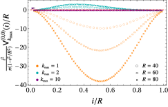
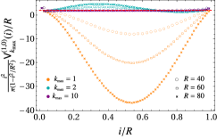
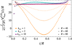
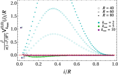
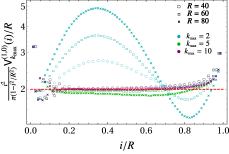
Figure 15: Combination (3.18) when $\omega=0$ in the case of $d=3$, for different values of $k_{\textrm{\tiny{max}}}$. The dashed red horizontal lines correspond to $\mu_{3}(l)=l(l+1)$, i.e. (2.11) when $d=3$. These panels should be compared with the right panels of Fig. 4.

References

- [1] L. Bombelli, R. K. Koul, J. Lee and R. D. Sorkin, “A Quantum Source of Entropy for Black Holes”, Phys. Rev. D 34, 373 (1986).
- [2] M. Srednicki, “Entropy and area”, Phys. Rev. Lett. 71, 666 (1993), hep-th/9303048.
- [3] C. G. Callan, Jr. and F. Wilczek, “On geometric entropy”, Phys. Lett. B 333, 55 (1994), hep-th/9401072.
- [4] C. Holzhey, F. Larsen and F. Wilczek, “Geometric and renormalized entropy in conformal field theory”, Nucl. Phys. B 424, 443 (1994), hep-th/9403108.
- [5] G. Vidal, J. I. Latorre, E. Rico and A. Kitaev, “Entanglement in quantum critical phenomena”, Phys. Rev. Lett. 90, 227902 (2003), quant-ph/0211074.
- [6] P. Calabrese and J. L. Cardy, “Entanglement entropy and quantum field theory”, J. Stat. Mech. 0406, P06002 (2004), hep-th/0405152.
- [7] J. Eisert, M. Cramer and M. Plenio, “Area laws for the entanglement entropy - a review”, Rev. Mod. Phys. 82, 277 (2010), arxiv:0808.3773.
- [8] V. Eisler and I. Peschel, “Reduced density matrices and entanglement entropy in free lattice models”, J. Phys. A 42, 504003 (2009), arxiv:0906.1663.
- [9] H. Casini and M. Huerta, “Entanglement entropy in free quantum field theory”, J. Phys. A 42, 504007 (2009), arxiv:0905.2562.
- [10] J. Bisognano and E. Wichmann, “On the Duality Condition for a Hermitian Scalar Field”, J. Math. Phys. 16, 985 (1975).
- [11] J. Bisognano and E. Wichmann, “On the Duality Condition for Quantum Fields”, J. Math. Phys. 17, 303 (1976).
- [12] P. D. Hislop and R. Longo, “Modular Structure of the Local Algebras Associated With the Free Massless Scalar Field Theory”, Commun. Math. Phys. 84, 71 (1982).
- [13] H. Casini, M. Huerta and R. C. Myers, “Towards a derivation of holographic entanglement entropy”, JHEP 1105, 036 (2011), arxiv:1102.0440.
- [14] R. Haag, “Local quantum physics: Fields, particles, algebras”, Springer (1996).
- [15] G. Wong, I. Klich, L. A. Pando Zayas and D. Vaman, “Entanglement Temperature and Entanglement Entropy of Excited States”, JHEP 1312, 020 (2013), arxiv:1305.3291.
- [16] J. Cardy and E. Tonni, “Entanglement hamiltonians in two-dimensional conformal field theory”, J. Stat. Mech. 1612, 123103 (2016), arxiv:1608.01283.
- [17] E. Tonni, J. Rodríguez-Laguna and G. Sierra, “Entanglement hamiltonian and entanglement contour in inhomogeneous 1D critical systems”, J. Stat. Mech. 1804, 043105 (2018), arxiv:1712.03557.
- [18] I. Peschel, “Calculation of reduced density matrices from correlation functions”, J. Phys. A 36, L205 (2003), cond-mat/0212631.
- [19] I. Peschel, “On the reduced density matrix for a chain of free electrons”, J. Stat. Mech. 2004, P06004 (2004), cond-mat/0403048.
- [20] L. Banchi, S. L. Braunstein and S. Pirandola, “Quantum fidelity for arbitrary Gaussian states”, Phys. Rev. Lett. 115, 260501 (2015), arxiv:1507.01941.
- [21] R. Arias, D. Blanco, H. Casini and M. Huerta, “Local temperatures and local terms in modular Hamiltonians”, Phys. Rev. D 95, 065005 (2017), arxiv:1611.08517.
- [22] V. Eisler and I. Peschel, “Analytical results for the entanglement Hamiltonian of a free-fermion chain”, J. Phys. A 50, 284003 (2017), arxiv:1703.08126.
- [23] V. Eisler and I. Peschel, “Properties of the entanglement Hamiltonian for finite free-fermion chains”, J. Stat. Mech. 1810, 104001 (2018), arxiv:1805.00078.
- [24] V. Eisler, E. Tonni and I. Peschel, “On the continuum limit of the entanglement Hamiltonian”, J. Stat. Mech. 1907, 073101 (2019), arxiv:1902.04474.
- [25] G. Di Giulio and E. Tonni, “On entanglement hamiltonians of an interval in massless harmonic chains”, J. Stat. Mech. 2003, 033102 (2020), arxiv:1911.07188.
- [26] V. Eisler, G. Di Giulio, E. Tonni and I. Peschel, “Entanglement Hamiltonians for non-critical quantum chains”, J. Stat. Mech. 2010, 103102 (2020), arxiv:2007.01804.
- [27] I. Peschel and T. T. Truong, “Corner Transfer Matrices for the Gaussian Model”, Annalen der Physik 503, 185 (1991).
- [28] I. Peschel and M.-C. Chung, “Density matrices for a chain of oscillators”, J. Phys. A 32, 8419 (1999), cond-mat/9906224.
- [29] A. Erdelyi, “Higher Transcendental Functions”, McGraw Hill, New York (1953).
- [30] M. Abramowitz and I. A. Stegun, “Handbook of Mathematical Functions”, Dover, New York (1972).
- [31] C. Frye and C. J. Efthimiou, “Spherical Harmonics in p Dimensions”, arxiv:1205.3548.
- [32] A. Liguori and M. Mintchev, “Quantum field theory, bosonization and duality on the half line”, Nucl. Phys. B 522, 345 (1998), hep-th/9710092.
- [33] K. Audenaert, J. Eisert, M. Plenio and R. Werner, “Entanglement Properties of the Harmonic Chain”, Phys. Rev. A 66, 042327 (2002), quant-ph/0205025.
- [34] M. Cramer, J. Eisert, M. Plenio and J. Dreissig, “An Entanglement-area law for general bosonic harmonic lattice systems”, Phys. Rev. A 73, 012309 (2006), quant-ph/0505092.
- [35] M. Cramer and J. Eisert, “Correlations, spectral gap and entanglement in harmonic quantum systems on generic lattices”, New Journal of Physics 8, 71–71 (2006), quant-ph/0509167.
- [36] P. Calabrese, J. Cardy and E. Tonni, “Entanglement negativity in extended systems: A field theoretical approach”, J. Stat. Mech. 1302, P02008 (2013), arxiv:1210.5359.
- [37] A. Botero and B. Reznik, “Spatial structures and localization of vacuum entanglement in the linear harmonic chain”, Phys. Rev. A 70, 052329 (2004), quant-ph/0403233.
- [38] V. P. Frolov, P. Sutton and A. Zelnikov, “The Dimensional reduction anomaly”, Phys. Rev. D 61, 024021 (2000), hep-th/9909086.
- [39] A. A. Saharian, “Scalar Casimir effect for D-dimensional spherically symmetric Robin boundaries”, Phys. Rev. D 63, 125007 (2001), hep-th/0012185.
- [40] A. Riera and J. I. Latorre, “Area law and vacuum reordering in harmonic networks”, Phys. Rev. A 74, 052326 (2006), quant-ph/0605112.
- [41] R. Lohmayer, H. Neuberger, A. Schwimmer and S. Theisen, “Numerical determination of entanglement entropy for a sphere”, Phys. Lett. B 685, 222 (2010), arxiv:0911.4283.
- [42] M. Huerta, “Numerical Determination of the Entanglement Entropy for Free Fields in the Cylinder”, Phys. Lett. B 710, 691 (2012), arxiv:1112.1277.
- [43] H. Liu and M. Mezei, “A Refinement of entanglement entropy and the number of degrees of freedom”, JHEP 1304, 162 (2013), arxiv:1202.2070.
- [44] B. R. Safdi, “Exact and Numerical Results on Entanglement Entropy in (5+1)-Dimensional CFT”, JHEP 1212, 005 (2012), arxiv:1206.5025.
- [45] I. R. Klebanov, T. Nishioka, S. S. Pufu and B. R. Safdi, “Is Renormalized Entanglement Entropy Stationary at RG Fixed Points?”, JHEP 1210, 058 (2012), arxiv:1207.3360.
- [46] H. Casini and M. Huerta, “Entanglement entropy of a Maxwell field on the sphere”, Phys. Rev. D 93, 105031 (2016), arxiv:1512.06182.
- [47] J. S. Cotler, M. P. Hertzberg, M. Mezei and M. T. Mueller, “Entanglement Growth after a Global Quench in Free Scalar Field Theory”, JHEP 1611, 166 (2016), arxiv:1609.00872.
- [48] T. Nishioka, “Entanglement entropy: holography and renormalization group”, Rev. Mod. Phys. 90, 035007 (2018), arxiv:1801.10352.
- [49] C. P. Herzog, “Universal Thermal Corrections to Entanglement Entropy for Conformal Field Theories on Spheres”, JHEP 1410, 028 (2014), arxiv:1407.1358.
- [50] M. Plenio, J. Eisert, J. Dreissig and M. Cramer, “Entropy, entanglement, and area: analytical results for harmonic lattice systems”, Phys. Rev. Lett. 94, 060503 (2005), quant-ph/0405142.
- [51] N. Schuch, J. I. Cirac and M. M. Wolf, “Quantum States on Harmonic Lattices”, Commun. Math. Phys. 267, 65–92 (2006), quant-ph/0509166.
- [52] C. Weedbrook, S. Pirandola, R. García-Patrón, N. J. Cerf, T. C. Ralph, J. H. Shapiro and S. Lloyd, “Gaussian quantum information”, Rev. Mod. Phys. 84, 621 (2012), arxiv:1110.3234.
- [53] S. N. Solodukhin, “Entanglement entropy of round spheres”, Phys. Lett. B 693, 605 (2010), arxiv:1008.4314.
- [54] M. P. Hertzberg and F. Wilczek, “Some Calculable Contributions to Entanglement Entropy”, Phys. Rev. Lett. 106, 050404 (2011), arxiv:1007.0993.
- [55] H. Casini and M. Huerta, “Entanglement entropy for the n-sphere”, Phys. Lett. B 694, 167 (2011), arxiv:1007.1813.
- [56] J. S. Dowker, “Hyperspherical entanglement entropy”, J. Phys. A 43, 445402 (2010), arxiv:1007.3865.
- [57] M. Smolkin and S. N. Solodukhin, “Correlation functions on conical defects”, Phys. Rev. D 91, 044008 (2015), arxiv:1406.2512.
- [58] L.-Y. Hung, R. C. Myers and M. Smolkin, “Twist operators in higher dimensions”, JHEP 1410, 178 (2014), arxiv:1407.6429.
- [59] C. P. Herzog and T. Nishioka, “The Edge of Entanglement: Getting the Boundary Right for Non-Minimally Coupled Scalar Fields”, JHEP 1612, 138 (2016), arxiv:1610.02261.
- [60] R. Longo and G. Morsella, “The massive modular Hamiltonian”, arxiv:2012.00565.
- [61] H. Casini and M. Huerta, “Reduced density matrix and internal dynamics for multicomponent regions”, Class. Quant. Grav. 26, 185005 (2009), arxiv:0903.5284.
- [62] R. Longo, P. Martinetti and K.-H. Rehren, “Geometric modular action for disjoint intervals and boundary conformal field theory”, Rev. Math. Phys. 22, 331 (2010), arxiv:0912.1106.
- [63] S. Hollands, “On the modular operator of mutli-component regions in chiral CFT”, Commun. Math. Phys. 384, 785 (2021), arxiv:1904.08201.
- [64] D. Blanco and G. Pérez-Nadal, “Modular Hamiltonian of a chiral fermion on the torus”, Phys. Rev. D 100, 025003 (2019), arxiv:1905.05210.
- [65] P. Fries and I. A. Reyes, “Entanglement Spectrum of Chiral Fermions on the Torus”, Phys. Rev. Lett. 123, 211603 (2019), arxiv:1905.05768.
- [66] M. Mintchev and E. Tonni, “Modular Hamiltonians for the massless Dirac field in the presence of a boundary”, JHEP 2103, 204 (2021), arxiv:2012.00703.
- [67] M. Mintchev and E. Tonni, “Modular Hamiltonians for the massless Dirac field in the presence of a defect”, JHEP 2103, 205 (2021), arxiv:2012.01366.
- [68] R. E. Arias, H. Casini, M. Huerta and D. Pontello, “Entropy and modular Hamiltonian for a free chiral scalar in two intervals”, Phys. Rev. D 98, 125008 (2018), arxiv:1809.00026.
- [69] X. Wen, S. Ryu and A. W. Ludwig, “Entanglement hamiltonian evolution during thermalization in conformal field theory”, J. Stat. Mech. 1811, 113103 (2018), arxiv:1807.04440.
- [70] G. Di Giulio, R. Arias and E. Tonni, “Entanglement hamiltonians in 1D free lattice models after a global quantum quench”, J. Stat. Mech. 1912, 123103 (2019), arxiv:1905.01144.
- [71] J. Lee, A. Lewkowycz, E. Perlmutter and B. R. Safdi, “Rényi entropy, stationarity, and entanglement of the conformal scalar”, JHEP 1503, 075 (2015), arxiv:1407.7816.
- [72] B. Nienhuis, M. Campostrini and P. Calabrese, “Entanglement, combinatorics and finite-size effects in spin chains”, J. Stat. Mech. 2009, P02063 (2009), arxiv:0808.2741.
- [73] P. Kim, H. Katsura, N. Trivedi and J. H. Han, “Entanglement and corner Hamiltonian spectra of integrable open spin chains”, Phys. Rev. B 94, 195110 (2016), arxiv:1512.08597.
- [74] M. Dalmonte, B. Vermersch and P. Zoller, “Quantum simulation and spectroscopy of entanglement Hamiltonians”, Nature Phys. 14, 827 (2018), arxiv:1707.04455.
- [75] J. Zhang, P. Calabrese, M. Dalmonte and M. A. Rajabpour, “Lattice Bisognano-Wichmann modular Hamiltonian in critical quantum spin chains”, SciPost Phys. Core 2, 7 (2020), arxiv:2003.00315.
- [76] F. Parisen Toldin and F. F. Assaad, “Entanglement Hamiltonian of Interacting Fermionic Models”, Phys. Rev. Lett. 121, 200602 (2018), arxiv:1804.03163.
- [77] A. M. Läuchli, “Operator content of real-space entanglement spectra at conformal critical points”, arxiv:1303.0741.
- [78] G. Torlai, L. Tagliacozzo and G. De Chiara, “Dynamics of the entanglement spectrum in spin chains”, J. Stat. Mech. 2014, P06001 (2014), arxiv:1311.5509.
- [79] V. Alba, P. Calabrese and E. Tonni, “Entanglement spectrum degeneracy and the Cardy formula in 1+1 dimensional conformal field theories”, J. Phys. A 51, 024001 (2018), arxiv:1707.07532.
- [80] J. Surace, L. Tagliacozzo and E. Tonni, “Operator content of entanglement spectra after global quenches in the transverse field Ising chain”, Phys. Rev. B 101, 241107 (2020), arxiv:1909.07381.
- [81] A. Roy, F. Pollmann and H. Saleur, “Entanglement Hamiltonian of the 1+1-dimensional free, compactified boson conformal field theory”, J. Stat. Mech. 2008, 083104 (2020), arxiv:2004.14370.
- [82] N. F. Robertson, J. Surace and L. Tagliacozzo, “On quenches to the critical point of the three states Potts model – Matrix Product State simulations and CFT”, arxiv:2110.07078.
- [83] Y. Chen and G. Vidal, “Entanglement contour”, J. Stat. Mech. 2014, P10011 (2014), arxiv:1406.1471.
- [84] I. Frérot and T. Roscilde, “Area law and its violation: A microscopic inspection into the structure of entanglement and fluctuations”, Phys. Rev. B 92, 115129 (2015), arxiv:1506.00545.
- [85] A. Coser, C. De Nobili and E. Tonni, “A contour for the entanglement entropies in harmonic lattices”, J. Phys. A 50, 314001 (2017), arxiv:1701.08427.
- [86] A. Peres, “Separability Criterion for Density Matrices”, Phys. Rev. Lett. 77, 1413–1415 (1996), quant-ph/9604005.
- [87] G. Vidal and R. F. Werner, “Computable measure of entanglement”, Phys. Rev. A 65, 032314 (2002), quant-ph/0102117.
- [88] M. B. Plenio, “Logarithmic Negativity: A Full Entanglement Monotone That is not Convex”, Phys. Rev. Lett. 95, 090503 (2005), quant-ph/0505071.
- [89] P. Calabrese, J. Cardy and E. Tonni, “Entanglement negativity in quantum field theory”, Phys. Rev. Lett. 109, 130502 (2012), arxiv:1206.3092.
- [90] P. Calabrese, L. Tagliacozzo and E. Tonni, “Entanglement negativity in the critical Ising chain”, J. Stat. Mech. 1305, P05002 (2013), arxiv:1302.1113.
- [91] P. Calabrese, J. Cardy and E. Tonni, “Finite temperature entanglement negativity in conformal field theory”, J. Phys. A 48, 015006 (2015), arxiv:1408.3043.
- [92] C. De Nobili, A. Coser and E. Tonni, “Entanglement entropy and negativity of disjoint intervals in CFT: Some numerical extrapolations”, J. Stat. Mech. 1506, P06021 (2015), arxiv:1501.04311.
- [93] V. Eisler and Z. Zimborás, “Entanglement negativity in two-dimensional free lattice models”, Phys. Rev. B 93, 115148 (2016), arxiv:1511.08819.
- [94] C. De Nobili, A. Coser and E. Tonni, “Entanglement negativity in a two dimensional harmonic lattice: Area law and corner contributions”, J. Stat. Mech. 1608, 083102 (2016), arxiv:1604.02609.
- [95] E. Caceres, S. Chapman, J. D. Couch, J. P. Hernandez, R. C. Myers and S.-M. Ruan, “Complexity of Mixed States in QFT and Holography”, JHEP 2003, 012 (2020), arxiv:1909.10557.
- [96] G. Di Giulio and E. Tonni, “Complexity of mixed Gaussian states from Fisher information geometry”, JHEP 2012, 101 (2020), arxiv:2006.00921.