Object-oriented implementation of algebraic multi-grid solver for lattice QCD on SIMD architectures and GPU clusters

Abstract

A portable implementation of elaborated algorithm is important to use variety of architectures in HPC applications. In this work we implement and benchmark an algebraic multi-grid solver for Lattice QCD on three different architectures, Intel Xeon Phi, Fujitsu A64FX, and NVIDIA Tesla V100, in keeping high performance and portability of the code based on the object-oriented paradigm. Some parts of code are specific to an architecture employing appropriate data layout and tuned matrix-vector multiplication kernels, while the implementation of abstract solver algorithm is common to all architectures. Although the performance of the solver depends on tuning of the architecture-dependent part, we observe reasonable scaling behavior and better performance than the mixed precision BiCGSstab solvers.

1 Introduction

Lattice QCD simulations have been one of the most challenging subjects in high performance computing in science. As increasing the precision of experimental data in elementary particle and nuclear physics, theoretical calculation is required to provide correspondingly precise predictions. Lattice QCD simulations are not only the first principle calculation of the strong interaction but also providing nonperturbative procedure to examine the candidates of new physics. A typical bottleneck in numerical simulations of lattice QCD is the linear equation for the Dirac fermion operator that is a large sparse matrix. As the simulated system becomes closer to the real system the linear equation becomes more difficult to solve because of larger lattice size and smaller quark mass parameter that increases the condition number. Therefore variety of improved algorithms have been developed for solving this linear equation. At the same time, numerous efforts have been devoted to exploit the new architecture of computers.

Multi-grid algorithms are widely used in solving large linear system. This type of algorithms applies coarsening of the lattice to define a matrix of smaller rank which reflects the long range effect of the original matrix while is easier to solve. The solution on the coarse lattice is used as a preconditioner of the original linear equation solver. A simple geometric coarsening, however, does not accelerate linear equation solvers in lattice QCD. It has been demonstrated that algebraic coarsening with adaptive setup is needed [1, 2, 3, 4, 5].

A direct trigger of this work is a need of porting the multi-grid algorithm to the supercomputer Fugaku [6] that has been installed at RIKEN Center for Computational Science (R-CCS) and provided for shared use recently. To make use of its potential arithmetic performance, one needs to implement a code that exploit the specific structure of the architecture. The A64FX architecture of Fugaku adopts the SIMD arithmetic operation in units of 512-bit length. While the same SIMD width is also adopted in the Intel AVX-512 instruction set architecture, their micro architectures are different, especially, in the instructions across the SIMD lanes needed for complex number arithmetics. Indeed different data layouts achieve better efficiency for the AVX-512 and A64FX architectures, as shown later.

Another important target of this work is GPU clusters, or systems with accelerator devices in general, which have been increasingly adopted as recent large-scale supercomputers. Such systems require heterogeneous parallelization code for the host processors and many-core devices. To implement the device kernel, several frameworks are available such as OpenACC, CUDA, and OpenCL. We adopt OpenACC in this work.

Under this situation, it is desirable to establish a code design that keeps machine specific implementation minimum while allows construction of algorithms in generic manner. The goal of this paper is to develop such a framework to implement the multi-grid algorithm applicable to various architectures exemplified for A64FX, Intel AVX-512, and an NVIDIA GPU cluster. To realize these contradicting issues, we adopt the object-oriented program design and specify the interface that the architecture specific code must provide. As a framework for implementation, we adopt a general purpose lattice QCD code set Bridge++ with extension to add a code that is tuned for specific architecture. We discuss how much the algorithm and optimization of code for specific architecture can be separated.

This paper is organized as follows. In the next section, we briefly introduce the linear equation in lattice QCD that is the target problem of this work. Section 3 summarizes the multi-grid algorithm implemented in this work. Section 4 describes our code implementation. Section 5 shows performance results measured on the following systems: Oakforest-PACS of JCAHPC (Intel Xeon Phi KNL cluster), Fugaku, and the Cygnus system at Univ. of Tsukuba (NVIDIA V100 cluster). The last section is devoted to conclusion and outlook.

2 Linear equation in lattice QCD simulations

In this section, we introduce the linear equation problem in lattice QCD simulations to least extent for understanding the following sections. For the formulation of lattice QCD and the principle of numerical simulation, there are many textbooks and reviews (e.g. [7]).

The lattice QCD is a field theory formulated on a four-dimensional Euclidean lattice. It consists of fermion (quark) fields and a gauge (gluon) field. The latter mediates interaction among quarks and are represented by ‘link variable’, $U_{\mu}(x)\in SU(3)$, where $x=(x_{1},x_{2},x_{3},x_{4})$ stands for a lattice site and $\mu=1,2,3,4$ is the spacetime direction. In numerical simulations the lattice size is finite: $x_{\mu}=1,2,\cdots,L_{\mu}$. The fermion field is represented as a complex vector on lattice sites, which carries 3 components of ‘color’ and 4 components of ‘spinor’, thus in total 12, degrees of freedom on each site. The dynamics of fermion is governed by a functional $S_{F}=\sum_{x,y}\psi^{\dagger}(y)D[U]^{-1}(x,y)\psi(y)$, where $D[U]$ is a fermion matrix acting on a fermion vector $\psi(x)$. A Monte Carlo algorithm is applied to generate an ensemble of the gauge field $\{U_{\mu}(x)\}$, that requires to solve a linear equation $x=D^{-1}\psi$ many times.

There is a variety of the fermion matrix $D[U]$ depending on the way to discretize the continuum theory. As a common feature, the matrix is sparse because of the locality of the interaction among quarks and gluons. In this paper, we examine the $O(a)$-improved Wilson fermion, also called clover fermion matrix,

$$D_{x,y}=[1+F(x)]\delta_{x,y}-\kappa\sum_{\mu=1}^{4}\left[(1-\gamma_{\mu})U_{\mu}(x)\delta_{x+\hat{\mu},y}+(1+\gamma_{\mu})U^{\dagger}_{\mu}(x-\hat{\mu})\delta_{x-\hat{\mu},y}\right],$$ (1)

where $x$, $y$ are lattice sites, $\hat{\mu}$ the unit vector along $\mu$-th axis, and the hopping parameter $\kappa=1/(8+2m_{0})$ related to the quark mass $m_{0}$. $F(x)$ is a $12\times 12$ Hermitian matrix made of link variables, which is introduced to reduce the finite lattice spacing artifact. As mentioned above, the link variable $U_{\mu}(x)$ is a $3\times 3$ complex matrix acting on the color and $\gamma_{\mu}$ is a $4\times 4$ matrix acting on the spinor degrees of freedom. Thus $D$ is a complex matrix of the rank $4\cdot 3L_{x}L_{y}L_{z}L_{t}$. It is standard to impose the periodic or anti-periodic boundary conditions.

As a general feature, as decreasing the quark mass $m_{0}$, the linear equation becomes more and more difficult to solve since the condition number of the matrix increases. Another general feature common to fermion matrices is so-called $\gamma_{5}$-Hermiticity, which is a remnant of the Hermiticity of fermion operator in the continuum theory:

$$D^{\dagger}=\gamma_{5}D\gamma_{5},\hskip 14.22636pt\gamma_{5}=-\gamma_{1}\gamma_{2}\gamma_{3}\gamma_{4}.$$ (2)

The byte-per-flop of the clover fermion is 0.94 for single precision arithmetics.

3 Multi-grid algorithm

This section describes the multi-grid algorithm applied in this paper. We first settle the convention to represent vectors. Adopting the style in the quantum mechanics, we denote a vector as $|x\rangle$ and its Hermitian conjugate $\langle x|$. They are vectors in the original fine lattice, and the vectors on coarse lattice is represented with suffix ‘c’, such as $|x\rangle_{c}$. For simplicity we describe a single level multi-grid algorithm, while a multi-level implementation is straightforward. The linear equation to be solved is

$$D|x\rangle=|b\rangle.$$ (3)

In the following, we first describe the general feature of the multi-grid algorithm and then technical details specific to the lattice QCD problem.

Solver algorithm with preconditioner.

The multi-grid algorithm works as a preconditioner of iterative Krylov subspace solvers. While there is a variety of choice for this outer solver, in this work we employ the BiCGStab algorithm with flexible preconditioner summarized as follows [9].

BiCGStab algorithm with flexible preconditioning

$|x\rangle:=|x_{0}\rangle,\hskip 5.69046pt|r\rangle:=|b\rangle-D|x_{0}\rangle$, $|\tilde{r}\rangle:=|r\rangle$, $|p\rangle=|r\rangle$

$M$ is the preconditioner and $|x_{0}\rangle$ is the given initial guess.

for $i$ = 0, …, $n$  do

$\alpha_{i}=\langle\tilde{r}|r_{i}\rangle/\langle\tilde{r}|DM|p_{i}\rangle$

$|x_{i}\rangle:=|x_{i}\rangle+\alpha_{i}M|p_{i}\rangle$, $|s_{i}\rangle:=|r_{i}\rangle-\alpha_{i}DM|p_{i}\rangle$

if($\bigl{|}|s_{i}\rangle\bigr{|}^{2}$ is small enough) break

$|t_{i}\rangle:=DM|s_{i}\rangle$,  $\omega_{i}:=\langle t_{i}|s_{i}\rangle/\langle t_{i}|t_{i}\rangle$

$|x_{i+1}\rangle:=|x_{i}\rangle+\omega_{i}M|r_{i}\rangle$,  $|r_{i+1}\rangle:=|s_{i}\rangle-\omega_{i}DM|s_{i}\rangle$

if($\bigl{|}|r_{i+1}\rangle\bigr{|}^{2}$ is small enough) break

$\beta_{i}=(\alpha_{i}/\omega_{i})\langle\tilde{r}|r_{i+1}\rangle/\langle\tilde{r}|r_{i}\rangle$,  $|p_{i+1}\rangle:=|r_{i+1}\rangle-\beta_{i}(|p_{i}\rangle-\omega_{i}D|p_{i}\rangle$

end

If the preconditioner $M$ provides an approximate solution, $Mx\sim D^{-1}x$, the algorithm works efficiently. As an example of such a preconditioner, multi-precision solver is known to work efficiently, in particular on a system whose performance is regulated by its memory bandwidth. The version of algorithm we use has two break points as described above.

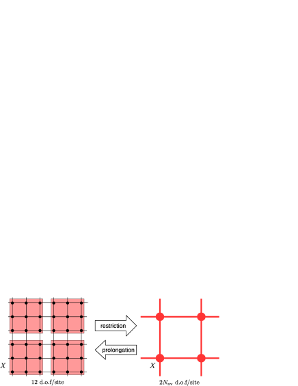
Figure 1: Schematic description of the multi-grid algorithm. A domain $X$ on the fine lattice is mapped to a site $X$ on the coarse lattice.

Multi-grid algorithm.

Figure 1 schematically explains the idea of the multi-grid algorithm. In some way we define the vectors on a coarser lattice, $|b\rangle\rightarrow|b\rangle_{c}$. This process is called ‘restriction’. Defining the matrix $D_{c}$ multiplied to this coarse vector correspondingly, one solves the linear equation

$$D_{c}|x\rangle_{c}=|b\rangle_{c}.$$ (4)

From this solution on the coarsened lattice, one can construct an approximate solution on the original fine lattice: $|x\rangle_{c}\rightarrow|x\rangle$ (called ‘prolongation’). This is a basic strategy of the multi-grid preconditioning. In addition, some operation called ‘smoothing’ is applied so as to improve the overlap of the approximate solution with the solution on the fine lattice, which contains the high frequency modes being not incorporated in the coarse solver. The smoother can be applied either before or after the coarse solver, or even both before and after.

Eq. (4) is easier to solve than the original linear equation due to its smaller rank, and to be solved not necessarily with high accuracy. In lattice QCD simulation, as quark mass decreases, the Dirac matrix $D$ becomes dominated by the low frequency modes that is well approximated by the coarse solution vector.

Construction of coarse grid operator.

To construct a coarse vector, we prepare $N_{\rm nv}$ so-called null space vectors that contain contribution from the low modes; $|i\rangle$, $i=1,\dots,N_{\rm nv}$. Since the quality of $|i\rangle$ governs the efficiency of the multi-grid preconditioner, we describe a way to generate them later in this section. Having prepared $|i\rangle$, we divide the original lattice into $N_{D}$ domains each composed of typically $4^{4}$ sites. Each domain, labeled with a capital letter as $X$, is mapped to one site on the coarse lattice. Let us express the $i$-th null space vector whose nonzero components are restricted to a domain $X$ as $|X,i\rangle$. At this stage we have totally $N_{\rm nv}N_{D}$ independent vectors. We further double the number of vectors effectively by applying projections in the 4-component ‘spin’ space into two subspaces labeled by $s=+,-$. The total number of independent vectors is thus $2N_{\rm nv}N_{D}$ which is labeled by $I=\{s,i,X\}$. Since these projections into domain $X$ and spin subspaces is local and almost trivial in the implementation, we need to keep only $N_{\rm nv}$ vectors $|i\rangle$.

Let us assume that vectors $2N_{\rm nv}N_{D}$ vectors $\{|I\rangle\}$ are orthonormalized: $\langle I|J\rangle=\delta_{IJ}$. Denoting the component of a coarse vector $|x\rangle_{c}$ as $x(I)$,

$$x(I)=\langle I|x\rangle.$$ (5)

This operation reduces the degrees of freedom from $12L_{x}L_{y}L_{z}L_{t}$ to $2N_{\rm nv}N_{D}$.

Prolongation is performed by

$$|x^{\prime}\rangle=\sum_{I}x(I)|I\rangle.$$ (6)

Note that $|x\rangle$ and $|x^{\prime}\rangle$ are in general different. The coarse Dirac fermion matrix $D_{c}(I,J)$ is represented as

$$D_{c}=\langle I|D|J\rangle.$$ (7)

Numerical steps.

To summarize with a little more details, the multi-grid preconditioner is composed of the following steps.

(0) Building of null space vectors (setup stage)

(0-a) Initial setup:

We start with $N_{\rm nv}$ independent random vectors. In general, multiplying an approximate $D^{-1}$ amplifies low frequency modes. For this purpose, several iterations of arbitrary iterative solver algorithm may suffice. Instead of simply using $D$ on fine lattice, we employ the Schwartz alternating procedure explained below. After the vectors are orthonormalized to $\langle I|J\rangle=\delta_{IJ}$, the coarse Dirac matrix $D_{c}$ is determined accordingly to Eq. (7).

(0-b) Adaptive improvement:

Once the initial null space vectors and coarse matrix are prepared, we use the multi-grid preconditioner itself (steps (1)–(2) bellow) as an approximate $D^{-1}$ to further amplify the low frequency modes in the null space vectors. The coarse matrix is simultaneously updated accordingly. This improvement process may be repeated several times.

Provided the null space vectors and coarse matrix, we employ the following multi-grid preconditioner. Each step is a Richardson refinement, $|x\rangle+M_{i}(|b\rangle-D|x\rangle)\mapsto|x\rangle$ with $M_{i}\simeq D^{-1}$ ($i=1,2$).

(1) Refinement on the coarse grid:

The approximate solver $M_{1}$ is made of the following three steps.

(1a) Restriction:

For a given source vector for the preconditioner, Eq. (5) is applied to make a vector on coarse lattice.

(1b) Coarse matrix solver:

The linear equation on coarse lattice (4) is solved with a standard way. We employ the BiCGStab algorithm with an additional stabilization [8] in this work. This is not necessarily performed with high precision.

(1c) Prolongation:

The solution vector of Eq. (4) is prolonged to make a fine vector with Eq. (6). The prolonged vector is used in the refinement of approximate solution on the original lattice.

(2) Smoother:

We insert a smoother after the coarse grid refinement. As $M_{2}$ in the Richardson process, Schwartz Alternating Procedure (SAP) with fixed iterations is used in this work for which details are described below.

Note that once the null space vectors are obtained in the step (0a) and (0b), they are repeatedly used for different right hand side vectors $|b\rangle$.

Schwartz Alternating Procedure (SAP).

Schwartz alternating procedure helps to reduce the communication in solving large linear system. It was introduced in [10, 11] as a domain-decomposed preconditioner to the lattice QCD, and then used as an efficient smoother in the multi-grid algorithm [5].

One first divides the lattice into subdomains each containing e.g. $4^{4}$ sites which should be practically determined by observing the numerical efficiency. One defines the Dirac matrix $D_{\rm SAP}$ by turning off the interaction across the domains. This implies that if each domain lies within a node, inter-node communication does not exist in $D_{\rm SAP}$. We set the SAP domain to be the same as the domain of coarsening in the multi-grid algorithm. Splitting the domains into even and odd groups, $D_{\rm SAP}^{(e)}$ and $D_{\rm SAP}^{(o)}$, practical Schwartz alternating procedure is defined as follows.

Schwartz Alternating Procedure (SAP) with fixed iterations

$|x\rangle:=0,\hskip 5.69046pt|r\rangle:=|b\rangle$

for $i$ = 1, …, $n$  do

$|x\rangle:=|x\rangle+M_{\rm SAP}^{(e)}|r\rangle$

$|r\rangle:=|b\rangle-D|x\rangle$

$|x\rangle:=|x\rangle+M_{\rm SAP}^{(o)}|r\rangle$

$|r\rangle:=|b\rangle-D|x\rangle$

end

In this algorithm $M_{\rm SAP}^{(e/o)}$ is an inner-domain solver, $M_{\rm SAP}^{(e/o)}\simeq(D_{\rm SAP}^{(e/o)})^{-1}$. For this approximate solver, we adopt the MINRES algorithm with fixed number of iterations, 6. While the number of SAP iterations $n$ is one of the tuning parameters in the multi-grid algorithm, we set it to 4 in this work.

Related works.

Applications of the Multi-grid algorithms to lattice QCD have been developed in last 15 years [1, 2, 3]. Not only for the Wilson-type fermion matrix applied in this work, it is applied to the domain-wall fermion [4]. The SAP is introduced to the multi-grid algorithm in Ref. [5]. Their implementation was ported to K-computer [12]. As for the optimization for recent architecture, application to the Xeon Phi series is investigated [13]. Among widely used lattice QCD code sets, Grid [14, 15] contains a branch with multi-grid solvers. QUDA [16, 17], which is a lattice QCD library on GPUs, also contains multi-grid solvers. The data layout for Fugaku in the current work is a generalization of a solver library (not multi-grid) for Fugaku [18].

4 Implementation

4.1 Multi-grid algorithm

To apply the multi-grid algorithm to variety of computer architecture, it is desirable to separate the algorithm and code implementation on specific architecture as much as possible. A guideline to accomplish it is the so-called object-oriented programming. As a code framework, we employ a general purpose lattice QCD code set Bridge++ [19, 20] which is written in C++ based on the object-oriented design. Bridge++ has been used to investigate a recipe of tuning on Intel AVX-512 architectures [21, 22].

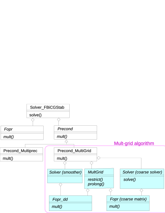
Figure 2: Class diagram for the multi-grid algorithm. The objects of classes in blue color are implemented in single precision arithmetics.

Figure 2 displays a simplified class diagram of our implementation. All the classes are implemented as C++ template class for which a template parameter AField is omitted in the Figure. AField itself is a template class that holds field data with specific precision and architecture such as AField<float, SIMD>, where the second template parameter is an enum entry. The objects in the blue colored classes are constructed with single precision arithmetics. We show only the abstract classes except for the top level solver (BiCGStab algorithm with flexible preconditioning) and two subclasses of the preconditioner, Precond. One may choose a multi-precision solver as a preconditioner instead of the multi-grid algorithm.

Most of the ingredients of multi-grid algorithm is implemented independently of the fermion matrix and architecture. For a specific fermion matrix, e.g. the clover fermion in this work, one needs to implement subclasses of Fopr and Fopr_dd, where the latter represents a domain-decomposed version of the former. One can apply optimization for the specific architecture to this implementation. While the smoother is represented as an abstract Solver class and can be any solver, we use SAP solver in this work. In a subclass of MultiGrid class, functions for restriction and prolongation are implemented for the specific fermion matrix. A blocked version of linear algebra is used in these operations. Such blocked linear algebraic functions may effect the performance significantly and thus are implemented as a functional template code for each architecture.

In the case of the clover fermion, we therefore need to implement three objects in addition to the standard fermion matrix: the domain-decomposed version of the fermion matrix (AFopr_Clover_dd class), the matrix on the coarse lattice (AFopr_Clover_coarse class), and a set of blocked version of linear algebraic functions such as dotc and axpy. The last ingredients are provided as C++ template functions. These parts are possible to optimize independently from the construction of the algorithm. In the following, we summarize the features of our target architectures and procedures of tuning.

4.2 Implementation for Intel AVX-512 architecture

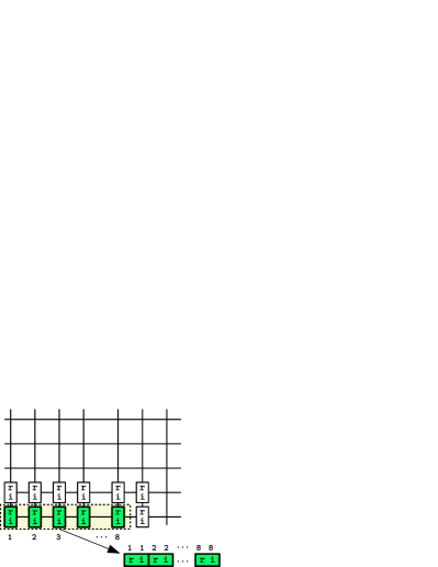
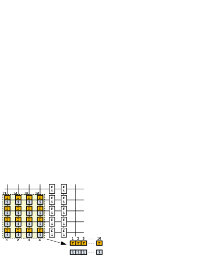
Figure 3: The SIMD layouts for the AVX-512 (left panel) and A64FX (right) architectures. In the figure, r and i represent real and imaginary part of a complex number on each lattice site, respectively. On the AVX-512, 8 complex numbers are packed to a SIMD variable while 16 complex numbers are packed to 2 SIMD variables (one for the real part and the other is the imaginary part) on the A64FX.

We start with the implementation of our multi-grid code for the Intel AVX-512 architecture. Intel AVX-512 is the latest SIMD extension of x86 instruction set architecture. The 512-bit SIMD length corresponds to 8 double or 16 single precision floating point numbers. In the following we consider the single precision case with which the preconditioner is implemented. We pack 8 complex numbers that are consecutive in the $x$-direction as displayed in the left panel of Figure 3. This implies that the size of the domain in $x$-direction is a multiple of 8 and it is indeed fixed to 8 in this work. For the coarse operator, we instead pack the internal degree of freedom to the SIMD variables to avoid a strong constraint on the local coarse lattice size. Since each coarse grid vector has $2N_{\rm nv}$ complex components, $N_{\rm nv}$ is constrained to be a multiple of 4.

The implementation of the fine grid operators inherits the previous works [21, 22] and uses the L2 prefetch in the full operator $D$. Although it has been tuned for $D$, the same prefetching pattern is used in the SAP operator.

4.3 Implementation for A64FX architecture

After the success of K computer, RIKEN decided to develop the post-K computer as a massively parallel computer with the Arm instruction set architecture with scalable vector extension (SVE). The development has successfully resulted in the Fugaku supercomputer manufactured by Fujitsu that has been installed at RIKEN R-CCS and provided for shared use since March 2021. In addition to Fugaku, there are several systems with the same architecture. The A64FX architecture adopted in Fugaku has 512-bit SIMD length that amounts to 16 single precision floating point numbers. The SIMD instructions are directly specified in a C/C++ code through ACLE (Arm C Language Extension).

The linear equation solver for the Dirac matrix in lattice QCD simulation has been one of the target applications in the development of the Post-K project that has lead to the Fugaku supercomputer. As a product of so-called co-design study, an optimized code named QWS (QCD Wide SIMD) library has been developed [18]. Through this investigation, it has been found that better performance is achieved by treating the real and imaginary parts in different SIMD vectors. Simplest implementation is achieved by packing 16 sites in $x$-direction into one SIMD vector for FP32, as adopted in the QWS library. For the implementation of the multi-grid algorithm, however, this implies that the domain size would be multiple of 16 at least in $x$-direction. This is rather strong restriction for examining the efficiency of the algorithm. Thus we decided to develop another code that packs the sites in $x$-$y$ plane as depicted in the right panel of Figure 3. This enables for example to pack $4\times 4$ sites into a single SIMD vector for FP32 and increases the flexibility in choosing the parameters.

We develop a library of fermion matrices with the above 2D SIMD packing and with the same convention and data layout as QWS. Tuning of this library is still underway by employing ACLE by making use of the techniques established in the development of QWS.

4.4 Implementation for GPU clusters

In implementation of a code for GPU, the first question is which offloading scheme is to be adopted. Two types of approaches are available: API-based libraries (CUDA, OpenCL, etc.) and directive-based ones (OpenACC and OpenMP). The former enables detailed manipulation of threads as well as the use of local store shared by a set of device cores. The latter is easy to start and suitable for incremental development. After preparatory study by comparing OpenCL and OpenACC, Bridge++ adopted to develop the offloading code mainly using OpenACC because of its simplicity and less effort in maintaining the code.

For the fermion matrix on original lattice, we assign the operations on each site to one device thread. The data layout is changed so that the so-called coalesced memory access is realized on the devices. For the matrix-vector multiplication on coarse lattice, computation of the vector component corresponding to one null space vector on each coarse site is assigned to one thread. In the case of GPU clusters, severe bottleneck is data transfer between the host processors and devices. Thus we implement a code that minimizes such data transfer and if necessary replace the general code with optimized code by exploiting the specialization of template in C++.

5 Performance result

We measure the performance of the multi-grid algorithm on the following three lattice sizes of gauge configurations labeled as A–C.

• A: $32^{3}\times 64$ lattice provided by PACS-CS collaboration [23].

• B: $64^{3}\times 64$ lattice provided by Yamazaki et al. [24].

• C: $96^{3}\times 96$ lattice provided by PACS collaboration [25].

These configurations are available through the Japan Lattice Data Grid [26, 27].

The block size for the multi-grid setup is fixed to $8\times 4^{3}$. The number of test vectors is set to 32 except for some benchmarks of matrix multiplications. Since these numbers should be tuned for each configurations, the throughput we investigate in this work may not be optimal. In addition to the solver, the performance of the matrix-vector multiplications is examined in the weak scaling setting, of which smaller local volume on Oakforest-PACS and Fugaku corresponds to running set A on 16 nodes.

For comparison, we also measure the elapsed time to solve the same system with a mixed precision BiCGStab solver. It uses the same flexible BiCGStab algorithm and the preconditioner is a single precision stabilized BiCGStab [8], the same algorithm used to solve the coarse system in the multi-grid solver.

Table 1: Elapsed time for the multi-grid solver. The ‘solve’ is for solving excluding the setup time. The ratios tabulated are time for solving the coarse solver, running the smoother, restriction and prolongation (R/P), and the other in the multi-grid preconditioner. For comparison, timing of mixed precision BiCGStab is also tabulated as ‘MBiCGs’. The block size is fixed to $8\times 4\times 4\times 4$. ‘OFP’ denotes Oakforest-PACS.

sys.	conf.	# of	$N_{\mathrm{nv}}$	elapsed time [sec]		fraction in the solve.				MBiCGs
	label	nodes		setup	solve	coarse	smoother	R/P	prec. other	[sec]
OFP	A	16	16	5.6	35	29%	53%	5.2%	7.6%	54
	A	16	32	16	23	62%	26%	4.5%	4.0%
	B	16	32	161	28	27%	50%	13%	5.9%	41
	B	32	32	65	13	28%	50%	11%	6.1%	22
	C	16	32	813	763	44%	35%	11%	4.8%	2801
	C	96	32	113	175	53%	29%	6.5%	5.5%	499
	C	192	32	60	80	51%	28%	5.6%	5.9%	297
Fugaku	A	16	32	107	31	33%	40%	19%	3.2%	121
	B	16	32	893	51	17%	48%	23%	6.6%	97
	C	96	32	688	213	34%	42%	18%	3.1%	1125
	C	216	32	314	111	41%	34%	18%	2.8%	512
Cygnus	A	1	32	500	198	50%	26%	20%	2.7%	—
	A	16	32	78	79	37%	13%	47%	1.7%	—
	B	16	32	263	21	23%	40%	27%	4.8%	—

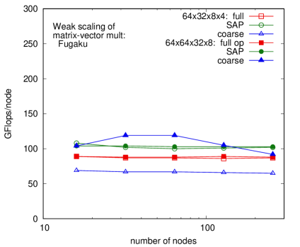
Figure 4: Weak scaling of matrix-vector multiplication on Oakforest-PACS (left panel) and Fugaku (right panel) with two different local lattice volumes, $5.2\times 10^{5}$ and $4.2\times 10^{6}$ lattice points per node. The matrices are full matrix $D$, domain decomposed operator $D_{\rm SAP}$ used in SAP in the smoother, and the coarse operator used in the coarse solver. The block size is $8\times 4\times 4\times 4$ and number of null space vector $N_{\rm nv}$ is 32.

5.1 Performance on Intel Xeon Phi cluster

We use the Oakforest-PACS system of JCAHPC. The compiler is Intel compiler 2019.5 and the option used is -O3 -no-prec-div -axMIC-AVX512. We use cache mode of the MCDRAM and set the number of the thread to 2 per core.

In the left panel of Figure 4, the weak scaling of the matrix-vector multiplication is plotted in two cases of local volume. For the smaller local volume case, the domain-decomposed operator is faster than the full operator as expected from the absence of communications. The tuning described in [22] for full operator works quite efficiently for a larger local volume so that its performance exceeds that of the domain-decomposed operator. Note that a naive roof line limit of the full operator is about 450 GFlops. The coarse operator is slower than the others. This is because the local volume is smaller than the fine lattice so that the cost of the neighboring communication becomes relatively larger, in addition to the lack of detailed tuning such as prefetching.

The elapsed time and time budget are listed in Table 1. Once the null space vectors are prepared (‘setup’), the multi-grid algorithm is faster than the mixed-precision solver. However, the overhead of setup becomes not negligible as the condition number decreases, as exhibited for configuration B. The fraction of the coarse solver and smoother depends on the configuration and the number of nodes, while the remaining part of the preconditioner including the restriction/prolongation is kept small. The performance of the multi-grid solver is 120–190 GFlops per node, which depends on the size of local volume and the fraction of the coarse grid solver.

5.2 Performance on Fugaku

On Fugaku, we use the Fujitsu compiler with the Clang mode. The version of the compiler is 1.2.31 and the option is -Nclang -fopenmp -Ofast. When we measured the performance, May 2021, jobs with a small number of nodes ($<385$) are not guaranteed to have physically close allocation in the 6-dimensional mesh-torus network. In this setting, frequent neighboring communication of the matrix multiplication kernel of QCD may interfere with communication of other jobs. We therefore secure a large enough number of nodes for which continuous torus geometry is guaranteed and then use a subset of them by specifying a rank map.

The performance of each matrix-vector multiplication is plotted in the right panel of Figure 4. There is plenty of room for improvement, since the node of Fugaku has roughly the same peak performance as Oakforest-PACS and larger memory bandwidth. Note the difference of the scale between panels in the figure. The SAP operator is fastest than the full operator as expected. Although the code is still in the middle of tuning, the coarse operator with larger local volume sometimes outperforms the SAP operator. All kernels show a good weak scaling.

The elapsed time and time budget are listed in Table 1. Compared with Oakforest-PACS, restriction and prolongation take larger fractions. This is because we have applied ACLE tuning to only a part of matrix vector multiplication, and the linear algebraic functions have still not been tuned. The solving time is shorter than the mixed precision BiCGStab solver in all cases. Taking the setup time into account, the latter is faster for configurations A and B. Note that once the setup is finished, one can solve the linear equation with different right hand sides repeatedly, which is a typical situation in lattice QCD simulation. In such a case, the multi-grid solver may become an efficient solution. The total performance of the solver is 83 – 96 GFlops per node, which is in between the performance of coarse matrix and $D_{\rm SAP}$.

5.3 Performance on GPU cluster

As an example of GPU cluster, we use the Cygnus system at University of Tsukuba. Each node of Cygnus is composed of two Intel Xeon processors (Xeon Gold 6126, 12 cores/2.6 GHz) and four NVIDIA Tesla V100 GPUs. Although 32 nodes of Cygnus have FPGA devices connected with dedicated network, we do not use this type of nodes. Each V100 GPU has 5120 CUDA cores which amounts to 14 TFlops for FP32 arithmetics. The memory bandwidth of the GPU global memory is 900 GB/s. The bus interface is PCIe 3.0 with 16 lanes. The nodes are connected by Infiniband HDR100 x4 network. We use the NVIDIA HPC SDK 20.9 compiler with CUDA 11.0 and the MPI library MVAPICH2-GDR 2.3.5. The code is compiled with options -O2 -ta=tesla:ptxinfo,cc70. We found that -fast option rather decreases the performance of the device kernel. Since most arithmetically heavy operations are performed on GPUs, multi-threading on the host processor contributes the performance little, and thus we switched it off in this measurement.

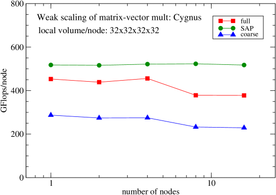
Figure 5: Weak scaling plot of the performance of matrix-vector multiplications on Cygnus. The local volume per node is set to $32^{4}$.

Figure 5 displays the weak scaling plot of the performance of matrix-vector multiplications for $D$ (full), $D_{\rm SAP}$, and coarse matrix $D_{c}$ in single precision. To keep large enough local volume even after the coarsening, we measure the performance with lattice size per node $32^{4}$. This lattice is divided to four GPU devices on each node. We observe that the performances of $D$ and coarse matrix decrease about 15% between 4 and 8 nodes while that of $D_{\rm SAP}$ stays unchanged, as the effect of changing the MPI parallelization in $(x,y)$ to $(x,y,z)$ directions. Considering the device memory bandwidth above and the byte-per-flop of the matrix $D$, 0.94, further optimization may be possible. For this purpose, CUDA or OpenCL would be required to employ for more detailed tuning.

The elapsed time and time budget are listed in Table 1. The configuration C is not available due to insufficient memory size of the maximum number of nodes (16) in our budget. On Cygnus, we do not measure the mixed-precision solver due to the lack of time for preparation. General tendency of the time budget in the multi-grid algorithm is similar to the SIMD architectures. The fractions of restriction and prolongation, however, tend to be larger due to the data transfer between the hosts and devices required for these steps in the current implementation. The result implies that the current implementation is also efficient for the architecture with GPU accelerators.

6 Conclusion

In this paper, we implemented a multi-grid solver for lattice QCD on two SIMD architectures and GPU clusters. On all the architectures, the multi-grid solver accomplished sufficient acceleration of elapsed time in solving linear equation under typical parameter setup. Although setup of the null space vector requires non-negligible time, once they are prepared, solving the linear equation for each source vector is significantly accelerated. In the measurement of physical quantities in lattice QCD simulations, one frequently encounters the situation to repeat such processes, for which the multi-grid algorithm would be a powerful solution.

By separating the architecture-specific code from the construction of algorithm, it has become possible to tune for each architecture independently. While present implementation is not very optimized, one can concentrate on each architecture for individual requirement. In this paper, we focus on one type of fermion matrix. Application to other type of matrix, such as the domain-wall fermion, is underway. Application to other recent architectures, such as the NEC SX-Aurora TSUBASA with vector architecture, is also planned.

References

- [1] Brannick, J., Brower, R. C., Clark, M. A., Osborn, J. C., Rebbi, C.: Adaptive Multigrid Algorithm for Lattice QCD. Phys. Rev. Lett. 100, 041601 (2008). doi:10.1103/PhysRevLett.100.041601
- [2] Babich, R., Brannick, J., Brower, R. C., Clark, M. A., Manteuffel, T. A., McCormick, S. F., Osborn, J. C., Rebbi, C.: Adaptive multigrid algorithm for the lattice Wilson-Dirac operator. Phys. Rev. Lett. 105, 201602 (2010). doi:10.1103/PhysRevLett.105.201602
- [3] Osborn, J. C., Babich, R., Brannick, J., Brower, R. C., Clark, M. A., Cohen, S. D., Rebbi, C.: Multigrid solver for clover fermions. PoS LATTICE2010, 037 (2010). doi:10.22323/1.105.0037
- [4] Cohen, S. D., Brower, R. C., Clark, M. A., Osborn, J. C.: Multigrid Algorithms for Domain-Wall Fermions. PoS LATTICE2011, 030 (2011). doi:10.22323/1.139.0030
- [5] Frommer, A., Kahl, K., Krieg,S., Leder, B., Rottmann, M.: Adaptive Aggregation Based Domain Decomposition Multigrid for the Lattice Wilson Dirac Operator. SIAM J. Sci. Comput. 36, A1581-A1608 (2014). doi:10.1137/130919507
- [6] Sato, M., et al.: Co-Design for A64FX Manycore Processor and ”Fugaku”. In: Proceedings of the International Conference for High Performance Computing, Networking, Storage and Analysis (SC ’20). IEEE Press, Article 47, 1–15 (2020).
- [7] Knechtli, F., Günther, M. Peardon, M.: Lattice Quantum Chromodynamics: Practical Essentials Springer Netherlands, Dordrect (2017). doi:10.1007/978-94-024-0999-4
- [8] Sleijpen, G. L. G., van der Vorst, H. A.: Maintaining convergence properties of BiCGstab methods in finite precision arithmetic. Numer. Algor. 10, 203-223 (1995). doi:10.1007/BF02140769
- [9] Vogel, J. A.: Flexible BiCG and flexible Bi-CGSTAB for nonsymmetric linear systems Appl. Math. Comput. 188, 226-233 (2007). doi:10.1016/j.amc.2006.09.116
- [10] Luscher, M.: Lattice QCD and the Schwarz alternating procedure. JHEP 05, 052 (2003). doi:10.1088/1126-6708/2003/05/052
- [11] Luscher, M.: Solution of the Dirac equation in lattice QCD using a domain decomposition method. Comput. Phys. Commun. 156, 209-220 (2004). doi:10.1016/S0010-4655(03)00486-7
- [12] Ishikawa, K. I., Kanamori, I.: Porting DDalphaAMG solver to K computer. PoS LATTICE2018, 310 (2018). doi:10.22323/1.334.0310
- [13] Georg, P., Richtmann, D., Wettig, T.: DD-AMG on QPACE 3. EPJ Web Conf. 175, 02007 (2018). doi:10.1051/epjconf/201817502007
- [14] Grid, https://github.com/paboyle/Grid
- [15] Boyle, P. A., Cossu, G, Yamaguchi, A. and Portelli, A.: Grid: A next generation data parallel C++ QCD library. PoS LATTICE2015, 023 (2016). doi:10.22323/1.251.0023
- [16] QUDA, https://github.com/lattice/quda
- [17] Clark, M. A., Babich, R., Barros, K., Brower, R. C. and Rebbi, C.: Solving Lattice QCD systems of equations using mixed precision solvers on GPUs. Comput. Phys. Commun. 181, 1517-1528 (2010). doi:10.1016/j.cpc.2010.05.002
- [18] QCD Wide SIMD library, https://github.com/RIKEN-LQCD/qws
- [19] Lattice QCD code set Bridge++, https://bridge.kek.jp/Lattice-code/
- [20] Ueda, S., Aoki, S., Aoyama, T., Kanaya, K., Matsufuru, H., Motoki, S., Namekawa, Y., Nemura, H., Taniguchi, Y. and Ukita, N.: Development of an object oriented lattice QCD code ’Bridge++. J. Phys. Conf. Ser. 523, 012046 (2014). doi:10.1088/1742-6596/523/1/012046
- [21] Kanamori, I., Matsufuru, H.: Practical Implementation of Lattice QCD Simulation on Intel Xeon Phi Knights Landing. Proceedings of the Fifth International Symposium on Computing and Networking (CANDAR’17), 19-22 November 2017, Aomori, Japan. doi:10.1109/CANDAR.2017.66
- [22] Kanamori, I., Matsufuru, H.: Practical Implementation of Lattice QCD Simulation on SIMD Machines with Intel AVX-512. Lecture Notes in Computer Science, 10962, 456-471 (2018). doi:10.1007/978-3-319-95168-3_31
- [23] Aoki, S. et al. [PACS-CS]: 2+1 Flavor Lattice QCD toward the Physical Point. Phys. Rev. D 79, 034503 (2009). doi:10.1103/PhysRevD.79.034503
- [24] Yamazaki.T, Ishikawa, K. I., Kuramashi, Y., Ukawa, A.: Helium nuclei, deuteron and dineutron in 2+1 flavor lattice QCD. Phys. Rev. D 86, 074514 (2012). doi:10.1103/PhysRevD.86.074514
- [25] Ishikawa, K. I. et al. [PACS]: 2+1 Flavor QCD Simulation on a Lattice. PoS LATTICE2015, 075 (2016). doi:10.22323/1.251.0075
- [26] Japan Lattice Data Grid, https://www.jldg.org/
- [27] Amagasa, T., Aoki, S., Aoki, Y., Aoyama, T., Doi, T., Fukumura, K., Ishii, N., Ishikawa, K. I, Jitsumoto, H., and Kamano, H. et al.: Sharing lattice QCD data over a widely distributed file system: J. Phys. Conf. Ser. 664, no.4, 042058 (2015). doi:10.1088/1742-6596/664/4/042058