Error estimates of the Godunov method for the multidimensional compressible Euler system

Abstract

We derive a priori error of the Godunov method for the multidimensional Euler system of gas dynamics. To this end we apply the relative energy principle and estimate the distance between the numerical solution and the strong solution. This yields also the estimates of the $L^{2}$-norm of errors in density, momentum and entropy. Under the assumption that the numerical density and energy are bounded, we obtain a convergence rate of $1/2$ for the relative energy in the $L^{1}$-norm. Further, under the assumption – the total variation of numerical solution is bounded, we obtain the first order convergence rate for the relative energy in the $L^{1}$-norm. Consequently, numerical solutions (density, momentum and entropy) converge in the $L^{2}$-norm with the convergence rate of $1/2$. The numerical results presented for Riemann problems are consistent with our theoretical analysis.

^∗,‡Institute of Mathematics, Johannes Gutenberg-University Mainz

Staudingerweg 9, 55 128 Mainz, Germany

lukacova@uni-mainz.de, yuhuyuan@uni-mainz.de

^†Academy for Multidisciplinary studies, Capital Normal University

West 3rd Ring North Road 105, 100048 Beijing, P. R. China

and

Institute of Mathematics of the Czech Academy of Sciences

Žitná 25, CZ-115 67 Praha 1, Czech Republic

she@math.cas.cz

Keywords: compressible Euler system, error estimates, relative energy, Godunov method, consistency formulation, strong solution

1 Introduction

We consider the Euler system governing the motion of a compressible gas

$$\partial_{t}{\bf U}+{\rm div}_{x}{\bf F}({\bf U})=0,\quad(t,x)\in(0,T)\times\Omega.$$ (1.1)

Here $\Omega\subset\mathbb{R}^{d}\,(d=1,2,3)$ is a bounded computational domain, ${\bf U}=(\varrho,{\bf m},E)^{T}$ represents the fluid density, momentum and total energy, while ${\bf F}$ is the flux function given by

$${\bf F}=({\bf m},{\bf u}\otimes{\bf m}+p\mathbb{I},{\bf u}(E+p))^{T}.$$

Here for positive $\varrho$, ${\bf u}=\frac{{\bf m}}{\varrho}$ is the velocity of the fluid and $p$ is the pressure satisfying the state equation of perfect gas

$$p=(\gamma-1)\varrho e,\quad\gamma\in(1,2]$$ (1.2)

with the specific internal energy $e=\frac{E}{\varrho}-\frac{1}{2}|{\bf u}|^{2}$.

We close the system with initial data

$${\bf U}(0,x)={\bf U}_{0}=(\varrho_{0},{\bf m}_{0}:=\varrho_{0}{\bf u}_{0},E_{0})$$ (1.3a)

satisfying

$$\varrho_{0}>0\quad\mbox{and}\quad E_{0}\in L^{1}(\Omega)$$ (1.3b)

and impermeability boundary condition

$${\bf u}\cdot{\bf n}|_{\partial\Omega}=0,$$ (1.4)

where ${\bf n}$ is the outer normal vector on the boundary $\partial\Omega$. Taking the Second law of Thermodynamics into account we further require that the entropy inequality holds, i.e.

$$\partial_{t}\,\eta({\bf U})+{\rm div}_{x}\,{\bf q}({\bf U})\geq 0.$$ (1.5)

Here $(\eta,{\bf q})$ is the physical entropy pair given by

$$\eta=C_{v}\varrho S,\quad{\bf q}=\eta{\bf u}\quad\mbox{with }C_{v}=\frac{1}{\gamma-1}\mbox{ and }S=\ln\left(\frac{p}{\varrho^{\gamma}}\right).$$ (1.6)

During the past few decades numerical simulation of the Euler system has been a hot topic in the field of computational mechanics and physics, cf. Toro [23], Feistauer et al. [10] , Li et al. [15], LeVeque [14]. Despite the success in practical simulations, a rigorous convergence analysis of the numerical methods still remains open in general. Most literature results were focused on scalar conservation laws. Kuznetsov [13] showed that the (upper) $L^{1}$ error bound is $\mathcal{O}(h^{1/2})$ for multi-dimensional scalar conservation laws under the assumptions on the boundedness of the total variation and continuity in time of numerical solutions, where $h$ is the mesh parameter. Further, Cockburn et al. [2] and Vila [24] extended the result of Kuznetsov and obtained the $L^{1}$-error bounds of ${\cal O}(h^{1/4})$ without the assumptions of bounded total variation and continuity in time. The convergence rate of some specific waves was also studied in one dimension. Concerning the linear advection equation, Tang and Teng [20] showed the sharpness of the $\mathcal{O}(\sqrt{\Delta x})$ $L^{1}$-error for monotone difference schemes with BV initial data. For the nonlinear scalar equation Teng and Zhang [22] showed the optimal convergence rate of $1$ in the $L^{1}$-norm for the viscosity method and monotone schemes if a solution is piecewise constant with finitely many shocks. Moreover, for the piecewise smooth entropy solution with finitely many rarefaction waves, Tang and Teng [21] showed that the error of viscosity solution to the inviscid solution is bounded by $\mathcal{O}(\varepsilon|\log\varepsilon|+\varepsilon)$ in the $L^{1}$-norm, where $\varepsilon$ denotes the viscosity coefficient. Furthermore, Tadmor and Tang [19] studied the pointwise error estimates and showed that the thicknesses of the shock and rarefaction layers are of order $\mathcal{O}(\varepsilon)$ and $\mathcal{O}(\varepsilon\log^{2}\varepsilon)$, respectively. We point out that the error estimates for scalar hyperbolic conservation laws are typically given in terms of the $L^{1}$-norm in space.

When considering the multidimensional nonlinear system of hyperbolic conservation laws, to our best knowledge, the only result was done by Jovanović and Rohde [12], where the convergence rate of $1/2$ was presented in terms of the $L^{2}$-errors between the numerical solutions and the classical solution $({\bf U}\in C^{1})$ under the assumption of uniform boundedness of numerical solutions and their $H^{1}$ semi-norm. In this paper we estimate the error between the numerical solutions and the strong solution $({\bf U}\in W^{1,\infty})$ assuming that the total variation of the numerical solution is bounded. Comparing with [12], we obtain the same convergence rate under a weaker assumption. Moreover, without the assumption of bounded total variation, we still have the convergence rate of $1/4$.

The main tool used in the paper is the so-called relative energy functional originally introduced by Dafermos [3]. This technique has been largely used in the analysis of the weak–strong uniqueness and singular limit of the compressible fluid flows, see the monograph of Feireisl and Novotný [9], Březina and Feireisl [1], and Feireisl et al. [7, 8]. Recently, this technique has also been successfully applied to the convergence analysis of numerical solutions of compressible viscous fluids, see Feireisl et al. [4] and Mizerová and She [17]. Here we adapt the technique to the Euler system and estimate the corresponding relative energy, which yields the control of the $L^{2}$-error of density, momentum and entropy, too.

The rest of the paper is organized as follows. In Section 2 we introduce some preliminaries. More precisely, we recall the Godunov method and its consistency formulation proved in Lukáčová and Yuan [16]. We define the strong solution of the Euler system and the relative energy. Further, we prove the relative energy inequality in Section 3 and estimate its error in the $L^{1}$-norm. Finally, in Section 4 we present some numerical experiments to validate theoretical results.

2 Preliminaries

In this section we introduce the preliminaries, including the formulation of the Godunov method, its consistency formulation, and the definitions of the strong solution and relative energy.

To begin, we define the following notations for the later use

$$\bullet\quad a\lesssim b\quad\mbox{ if }\quad a\leq cb\mbox{ with a positive constant c},$$

$$\bullet\quad a\approx b\quad\mbox{ if }\quad a\lesssim b\mbox{ and }b\lesssim a.$$

2.1 Godunov method

The computational domain $\Omega$ consists of rectangular meshes $\overline{\Omega}:=\bigcup_{K}\overline{K}$. We denote the set of all mesh cells as $\mathcal{T}_{h}$ and the set of all interior faces of $\mathcal{T}_{h}$ as $\Sigma_{\rm int}$. We consider the space of piecewise constant functions

$$\mathcal{Q}_{h}(\Omega)=\{v:v|_{K^{o}}=\mbox{constant},~{}\mbox{for all}~{}K\in\mathcal{T}_{h}\}$$ (2.1)

and define the projection operator

$$\Pi_{h}:L^{1}(\Omega)\rightarrow\mathcal{Q}_{h}(\Omega),\quad\Pi_{h}[\phi]_{K}=\frac{1}{|K|}\int_{K}\phi(x)~{}dx,$$ (2.2)

where $|K|$ is the Lebesgue measure of $K$.

Let ${\bf U}_{h}\in\mathcal{Q}_{h}(\Omega;\mathbb{R}^{d+2})$. Then the semi-discrete form of the finite volume method with the Godunov flux, i.e. the Godunov method can be described as

$$\int_{\Omega}\phi\frac{d}{dt}{\bf U}_{h}~{}\,{\rm d}{x}-\sum_{\sigma\in\Sigma_{\tt int}}\int_{\sigma}{\bf F}({\bf U}^{\it RP}_{\sigma})\cdot{\bf n}\left[\left[\phi\right]\right]~{}dS_{x}=0,$$ (2.3a)

$${\bf U}_{h0}=\Pi_{h}[{\bf U}_{0}].$$ (2.3b)

Here $\phi\in\mathcal{Q}_{h}(\Omega)$ is the test function, ${\bf U}^{\it RP}_{\sigma}$ is the exact solution of a local Riemann problem along the interface $\sigma$, and the notation $\left[\left[\cdot\right]\right]$ denotes the jump along the interface.

2.2 Consistency formulation

We recall the consistency formulation of the Godunov method derived by Lukáčová and Yuan [16]. We start with the following assumption.

Assumption 2.1.

We assume that the solution to (2.3) satisfies

$$0<\underline{\varrho}\leq\varrho_{h},\quad 0<E_{h}\leq\overline{E}\quad\mbox{uniformly for }h\rightarrow 0$$ (2.4)

for all $t\in[0,T]$, where $\underline{\varrho},\overline{E}$ are some positive constants.

Lemma 2.2.

Under Assumption 2.1 there hold

$$0<\underline{\varrho}\leq\varrho_{h}\leq\overline{\varrho},\quad|{\bf u}_{h}|\leq\overline{u},\quad 0<\underline{p}\leq p_{h}\leq\overline{p},~{}$$ (2.5)

$$|{\bf m}_{h}|\leq\overline{m},\quad 0<\underline{E}\leq E_{h}\leq\overline{E},\quad 0<\underline{\vartheta}\leq\vartheta_{h}\leq\overline{\vartheta}$$ (2.6)

uniformly for $h\rightarrow 0,t\in[0,T]$ with positive constants $\overline{\varrho},\,\overline{u},\,\underline{p},\,\overline{p},\,\overline{m},\,\underline{E},\,\underline{\vartheta},\,\overline{\vartheta}$ depending on $\underline{\varrho},\overline{E}$, where $\vartheta:=\frac{p}{\varrho}$ is the absolute temperature.

Theorem 2.3.

(Consistency formulation) Let $(\varrho_{h},{\bf m}_{h},\eta_{h})$ be the numerical solutions obtained by the Godunov method (2.3) on the time interval $[0,T]$ satisfying Assumption 2.1. Then for any $\tau\in(0,T)$ the following hold:

• for all $\phi\in W^{1,\infty}((0,T)\times\Omega)$

  $$\left[\int_{\Omega}\varrho_{h}\phi~{}\,{\rm d}{x}\right]_{t=0}^{t=\tau}=\int_{0}^{\tau}\int_{\Omega}\bigg{(}\varrho_{h}\partial_{t}\phi+{\bf m}_{h}\cdot\nabla_{x}\phi\bigg{)}\,{\rm d}{x}\,{\rm d}t+\int_{0}^{\tau}e_{\varrho,h}(t,\phi)\,{\rm d}t;$$ (2.7)

• for all $\boldsymbol{\phi}\in W^{1,\infty}((0,T)\times\Omega;\mathbb{R}^{d})$

  $$\left[\int_{\Omega}{\bf m}_{h}\cdot\boldsymbol{\phi}~{}\,{\rm d}{x}\right]_{t=0}^{t=\tau}= \int_{0}^{\tau}\int_{\Omega}\bigg{(}{\bf m}_{h}\cdot\partial_{t}\boldsymbol{\phi}+\frac{{\bf m}_{h}\otimes{\bf m}_{h}}{\varrho_{h}}:\nabla_{x}\boldsymbol{\phi}$$ (2.8)

  $$+p_{h}{\rm div}_{x}\boldsymbol{\phi}\bigg{)}\,{\rm d}{x}\,{\rm d}t+\int_{0}^{\tau}e_{{\bf m},h}(t,\boldsymbol{\phi})\,{\rm d}t;$$

• for all $\phi\in W^{1,\infty}((0,T)\times\Omega),\,\phi\geq 0$

  $$\left[\int_{\Omega}\eta_{h}\phi~{}\,{\rm d}{x}\right]_{t=0}^{t=\tau}\geq\int_{0}^{\tau}\int_{\Omega}\bigg{(}\eta_{h}\partial_{t}\phi+{\bf q}_{h}\cdot\nabla_{x}\phi\bigg{)}\,{\rm d}{x}\,{\rm d}t+\int_{0}^{\tau}e_{\eta,h}(t,\phi)\,{\rm d}t;$$ (2.9)

• $$\int_{\Omega}E_{h}(\tau)~{}\,{\rm d}{x}=\int_{\Omega}E_{0,h}~{}\,{\rm d}{x}$$ (2.10)

with bounded errors $e_{j,h},(j=\varrho,{\bf m},\eta)$ satisfying

$$\|e_{j,h}\|_{L^{1}(0,T)} \lesssim h\lVert\phi\rVert_{W^{1,\infty}((0,T)\times\Omega)}\int_{0}^{\tau}\sum_{\sigma\in\Sigma_{\tt int}}\int_{\sigma}\left|\left[\left[{\bf U}_{h}\right]\right]\right|~{}\mathrm{d}S_{x}\,{\rm d}t$$ (2.11)

$$\lesssim h^{1/2}\|\phi\|_{W^{1,\infty}((0,T)\times\Omega)}\left(\int_{0}^{\tau}\sum_{\sigma\in\Sigma_{\tt int}}\int_{\sigma}\left|\left[\left[{\bf U}_{h}\right]\right]\right|^{2}~{}\mathrm{d}S_{x}\,{\rm d}t\right)^{1/2}.$$

2.3 Strong solution

Our aim is to analyze the convergence rate of the Godunov method when approximating the strong solution of the Euler system (1.1)–(1.4).

Definition 2.4 (Strong solution).

Let $\Omega\subset\mathbb{R}^{d}$ be a bounded domain with a boundary $\partial\Omega$ of class $C^{1}$. We say that a trio $[\widetilde{\varrho},{\widetilde{\bf u}},{\widetilde{\eta}}]$ is the strong solution of the Euler system (1.1)–(1.4) if

$$\widetilde{\varrho}\in W^{1,\infty}((0,T)\times\Omega),$$

$${\widetilde{\bf u}}\in W^{1,\infty}((0,T)\times\Omega;\mathbb{R}^{d}),$$

$${\widetilde{\eta}}\in W^{1,\infty}((0,T)\times\Omega),$$

$$\widetilde{\varrho}>0\mbox{ and }\vartheta(\widetilde{\varrho},{\widetilde{\eta}})>0\ \mbox{for any}\ (t,x)\in[0,T]\times\overline{\Omega}$$

and the equations (1.1)–(1.4) are satisfied for almost everywhere.

Let us point out that we consider $\varrho$ and $\eta$ as the independent thermodynamical variables throughout the paper, meaning that all other thermodynamical variables are functions of $(\varrho,\eta)$. Accordingly, we write $\widetilde{v}=v(\widetilde{\varrho},{\widetilde{\eta}})$, $v\in\{p,e,\vartheta,S\}$, for the strong solution. Moreover, we denote $\widetilde{{\bf m}}=\widetilde{\varrho}{\widetilde{\bf u}}$ and $\widetilde{{\bf U}}={\bf U}(\widetilde{\varrho},{\widetilde{\bf u}},{\widetilde{\eta}})$.

Since the domain is bounded and $(\widetilde{\varrho},\widetilde{\vartheta})$ is continuous and positive, we have

$$0<\underline{\varrho}\leq\widetilde{\varrho},\quad 0<\underline{\vartheta}\leq\widetilde{\vartheta}.$$ (2.12)

Remark 2.5.

According to the definition of strong solution, we know that an entropy solution only containing finitely many rarefaction waves is also a strong solution.

We recall Gibbs’ relation

$$\widetilde{\vartheta}{\rm d}\widetilde{S}={\rm d}\widetilde{e}+\widetilde{p}~{}{\rm d}\left(1/\widetilde{\varrho}\right).$$ (2.13)

Consequently, for any strong solution $(\widetilde{\varrho},{\widetilde{\bf u}},{\widetilde{\eta}})$ we obtain the following identities which will be used in Section 3

$$\partial_{t}\widetilde{\varrho}+{\widetilde{\bf u}}\cdot\nabla_{x}\widetilde{\varrho}+\widetilde{\varrho}\,{\rm div}_{x}{\widetilde{\bf u}}=0,$$ (2.14)

$$\partial_{t}{\widetilde{\bf u}}+{\widetilde{\bf u}}\cdot\nabla_{x}{\widetilde{\bf u}}+\frac{1}{\widetilde{\varrho}}\,\nabla_{x}\widetilde{p}=0,$$

$$\partial_{t}{\widetilde{\eta}}+{\widetilde{\bf u}}\cdot\nabla_{x}{\widetilde{\eta}}+{\widetilde{\eta}}\,{\rm div}_{x}{\widetilde{\bf u}}=0,$$

$$\partial_{t}\widetilde{p}+{\widetilde{\bf u}}\cdot\nabla_{x}\widetilde{p}+\gamma\widetilde{p}\,{\rm div}_{x}{\widetilde{\bf u}}=0,$$

$$\partial_{t}\widetilde{S}+{\widetilde{\bf u}}\cdot\nabla_{x}\widetilde{S}=0,$$

$$\partial_{t}\widetilde{\vartheta}+{\widetilde{\bf u}}\cdot\nabla_{x}\widetilde{\vartheta}+\left(\partial_{{\widetilde{\eta}}}\widetilde{p}\right)_{\widetilde{\varrho}}{\rm div}_{x}{\widetilde{\bf u}}=0,$$

see [7, 23] for more details.

2.4 Relative energy

In this part we introduce the relative energy and show the relationship between the relative energy and the $L^{2}$-error of $(\varrho,{\bf m},\eta)$ for numerical solutions.

Let $(\varrho,{\bf m},\eta)$ and $(\widetilde{\varrho},{\widetilde{\bf u}},{\widetilde{\eta}})$ be two vectors consisting of density, momentum and velocity, respectively, and total entropy. In the context of the compressible Euler system, the relative energy reads

$${\mathbb{E}}\left(\varrho,{\bf m},\eta\Big{|}\widetilde{\varrho},{\widetilde{\bf u}},{\widetilde{\eta}}\right)=~{}\frac{1}{2}\varrho\left|\frac{{\bf m}}{\varrho}-{\widetilde{\bf u}}\right|^{2}+\varrho e-\frac{\partial(\varrho e)}{\partial\varrho}\Big{|}_{(\widetilde{\varrho},{\widetilde{\eta}})}(\varrho-\widetilde{\varrho})-\frac{\partial(\varrho e)}{\partial\eta}\Big{|}_{(\widetilde{\varrho},{\widetilde{\eta}})}(\eta-{\widetilde{\eta}})-\widetilde{\varrho}{\widetilde{e}}$$ (2.15)

for $\varrho>0$.

Lemma 2.6.

let $(\widetilde{\varrho},{\widetilde{\bf u}},{\widetilde{\eta}})$ be the strong solution of the Euler system in the sense of Definition 2.4 and let $(\varrho_{h},{\bf m}_{h},\eta_{h})$ be a numerical solution of the Euler system obtained by (2.3) satisfying Assumption 2.1. Then we have the following equivalence

$$\mathbb{E}\left(\varrho_{h},{\bf m}_{h},\eta_{h}\Big{|}\widetilde{\varrho},{\widetilde{\bf u}},{\widetilde{\eta}}\right)\approx|{\bf m}_{h}-\widetilde{{\bf m}}|^{2}+|\eta_{h}-{\widetilde{\eta}}|^{2}+|\varrho_{h}-\widetilde{\varrho}|^{2}.$$ (2.16)

Proof.

First, taking the derivatives of $\varrho e$ with respect to $(\varrho,\eta)$ we obtain

$$\partial_{\varrho}\left(\varrho e\right)=\left(1+C_{v}\right)\vartheta-\frac{\eta\vartheta}{\varrho},\quad\partial_{\eta}\left(\varrho e\right)=\vartheta.$$ (2.17)

Further, by the product rule and Gibbs’ relation (2.13) we derive

$${\rm d}\vartheta=\frac{\vartheta}{C_{v}\varrho}\left(1-\frac{\eta}{\varrho}\right){\rm d}\varrho+\frac{\vartheta}{C_{v}\varrho}{\rm d}\eta,$$ (2.18)

and

$${\rm d}\left((1+C_{v})\vartheta-\frac{\vartheta\eta}{\varrho}\right)=\left((1+C_{v})-\frac{\eta}{\varrho}\right){\rm d}\vartheta-\frac{\vartheta}{\varrho}{\rm d}\eta+\frac{\vartheta\eta}{\varrho^{2}}{\rm d}\varrho,$$ (2.19)

which leads to

$$\nabla_{(\varrho,\eta)}^{2}(\varrho e)=\frac{\vartheta}{C_{v}\varrho}\begin{pmatrix}1&1-\frac{\eta}{\varrho}\\ 1-\frac{\eta}{\varrho}&C_{v}+\left(1-\frac{\eta}{\varrho}\right)^{2}\end{pmatrix}.$$ (2.20)

As $(\varrho,{\bf u},\eta)$ is the strong solution we know that $\nabla_{(\varrho,\eta)}^{2}(\varrho e)|_{(\widetilde{\varrho},{\widetilde{\eta}})}$ is symmetric positive definite and bounded from below and above, which implies

$$\mathbb{E}\left(\varrho_{h},{\bf m}_{h},\eta_{h}\Big{|}\widetilde{\varrho},{\widetilde{\bf u}},{\widetilde{\eta}}\right) \approx|{\bf u}_{h}-{\widetilde{\bf u}}|^{2}+|\eta_{h}-{\widetilde{\eta}}|^{2}+|\varrho_{h}-\widetilde{\varrho}|^{2}.$$ (2.21)

Next, we recall Assumption 2.1 and the uniform upper bound of ${\bf u}_{h}$ due to Lemma 2.2 to conclude that

$$|{\bf m}_{h}-\widetilde{{\bf m}}|^{2}\leq|\varrho_{h}({\bf u}_{h}-{\widetilde{\bf u}})|^{2}+|(\varrho_{h}-\widetilde{\varrho}){\widetilde{\bf u}})|^{2}\lesssim|{\bf u}_{h}-{\widetilde{\bf u}}|^{2}+|\varrho_{h}-\widetilde{\varrho}|^{2},$$

$$|{\bf u}_{h}-{\widetilde{\bf u}}|^{2}\lesssim|\widetilde{\varrho}({\bf u}_{h}-{\widetilde{\bf u}})|^{2}\lesssim|{\bf m}_{h}-\widetilde{{\bf m}}|^{2}+|{\bf u}_{h}(\widetilde{\varrho}-\varrho_{h})|^{2}\lesssim|{\bf m}_{h}-\widetilde{{\bf m}}|^{2}+|\varrho_{h}-\widetilde{\varrho}|^{2}.$$

Substituting the above two inequalities into (2.21) we finish the proof. ∎

Lemma 2.6 means that the $L^{1}$-norm of $\mathbb{E}\left(\varrho_{h},{\bf m}_{h},\eta_{h}\Big{|}\widetilde{\varrho},{\widetilde{\bf u}},{\widetilde{\eta}}\right)$ is equivalent to the $L^{2}$-norm of the errors in $(\varrho_{h}-\widetilde{\varrho},{\bf m}_{h}-\widetilde{{\bf m}},\eta_{h}-{\widetilde{\eta}})$ as long as the entropy stable numerical solution $(\varrho_{h},{\bf m}_{h},\eta_{h})$ satisfies Assumption 2.1 and $(\widetilde{\varrho},{\widetilde{\bf u}},{\widetilde{\eta}})$ is the strong solution of the Euler system in the sense of Definition 2.4.

3 Error estimates

Equipped with consistency formulation of the Godunov method we are now ready to estimate the relative energy in the $L^{1}$-norm and error between the numerical solution $(\varrho_{h},{\bf m}_{h},\eta_{h})$ and the strong solution $(\widetilde{\varrho},{\widetilde{\bf u}},{\widetilde{\eta}})$ in the $L^{2}$-norm.

Theorem 3.1 (Error estimates).

Let $\Omega\subset\mathbb{R}^{d}$, $d=1,2,3,$ be a bounded domain with a boundary $\partial\Omega\in C^{1}$. Let $(\widetilde{\varrho},{\widetilde{\bf u}},{\widetilde{\eta}})$ be the strong solution of the complete Euler system (1.1) in the sense of Definition 2.4 with initial data (1.3) satisfying

$$\|{\bf U}_{h0}-{\bf U}_{0}\|_{L^{2}(\Omega)}\lesssim h^{1/2}$$

and the impermeability boundary condition (1.4).

Suppose that $(\varrho_{h},{\bf m}_{h},\eta_{h})$ is the numerical solution obtained by the Godunov method (2.3). Let Assumption 2.1 hold. Then the following estimate of the relative energy holds for any $\tau\in(0,T]$

$$\int_{\Omega}{\mathbb{E}}\left(\varrho_{h},{\bf m}_{h},\eta_{h}\Big{|}\widetilde{\varrho},{\widetilde{\bf u}},{\widetilde{\eta}}\right)(\tau,\cdot)\ \,{\rm d}{x}\\ \lesssim\exp\left(\tau\;c\left(\Omega,\|\widetilde{{\bf U}}\|_{W^{1,\infty}((0,T)\times\Omega;R^{d})}\right)\right)h^{1/2}.$$ (3.1)

Proof.

We prove (3.1) in two steps:

• Viewing $(\widetilde{\varrho},{\widetilde{\bf u}},{\widetilde{\eta}})$ as the test function in the consistency formulation, we derive the relative energy inequality between $(\varrho_{h},{\bf m}_{h},\eta_{h})$ and $(\widetilde{\varrho},{\widetilde{\bf u}},{\widetilde{\eta}})$;

• Approximating the above inequality such that all terms on the right hand side can be bounded by the discretization parameter $h$ or by the relative energy, we finally estimate the relative energy by Gronwall’s lemma.

Step 1.

Rewriting the relative energy (2.15) into a more convenient form we obtain

$${E}\left(\varrho_{h},{\bf m}_{h},\eta_{h}\Big{|}\widetilde{\varrho},{\widetilde{\bf u}},{\widetilde{\eta}}\right) =~{}\frac{1}{2}\varrho_{h}\left|\frac{{\bf m}_{h}}{\varrho_{h}}-{\widetilde{\bf u}}\right|^{2}+\varrho_{h}e_{h}-\left((1+C_{v})\widetilde{\vartheta}-\frac{\widetilde{\vartheta}{\widetilde{\eta}}}{\widetilde{\varrho}}\right)(\varrho_{h}-\widetilde{\varrho})-\widetilde{\vartheta}(\eta_{h}-{\widetilde{\eta}})-\widetilde{\varrho}{\widetilde{e}}$$ (3.2)

$$=\left[\frac{1}{2}\frac{|{\bf m}_{h}|^{2}}{\varrho_{h}}+\varrho_{h}e_{h}\right]+\varrho_{h}\left[\frac{1}{2}|{\widetilde{\bf u}}|^{2}-(1+C_{v})\widetilde{\vartheta}+\frac{\widetilde{\vartheta}{\widetilde{\eta}}}{\widetilde{\varrho}}\right]-{\bf m}_{h}\cdot{\widetilde{\bf u}}-\eta_{h}\widetilde{\vartheta}+{\widetilde{p}}.$$

First, we take $\frac{1}{2}|{\widetilde{\bf u}}|^{2}-(1+C_{v})\widetilde{\vartheta}+\frac{\widetilde{\vartheta}{\widetilde{\eta}}}{\widetilde{\varrho}}$ as the test function in consistency formulation of the density equation (2.7) to derive

$$\left[\int_{\Omega}\varrho_{h}\left(\frac{1}{2}|{\widetilde{\bf u}}|^{2}-(1+C_{v})\widetilde{\vartheta}+\frac{\widetilde{\vartheta}{\widetilde{\eta}}}{\widetilde{\varrho}}\right)~{}\,{\rm d}{x}\right]_{t=0}^{t=\tau}=\int_{0}^{\tau}\int_{\Omega}\Bigg{(}\varrho_{h}\partial_{t}\left(\frac{1}{2}|{\widetilde{\bf u}}|^{2}-(1+C_{v})\widetilde{\vartheta}+\frac{\widetilde{\vartheta}{\widetilde{\eta}}}{\widetilde{\varrho}}\right)$$

$$\quad+{\bf m}_{h}\cdot\nabla_{x}\left(\frac{1}{2}|{\widetilde{\bf u}}|^{2}-(1+C_{v})\widetilde{\vartheta}+\frac{\widetilde{\vartheta}{\widetilde{\eta}}}{\widetilde{\varrho}}\right)\Bigg{)}\,{\rm d}{x}\,{\rm d}t+\int_{0}^{\tau}e_{\varrho,h}(t,\widetilde{{\bf U}})\,{\rm d}t.$$

Analogously, we set ${\widetilde{\bf u}}$ and $\widetilde{\vartheta}$ respectively as the test functions in consistency formulations of the momentum equation (2.8) and entropy inequality (2.9) to get

$$\left[\int_{\Omega}{\bf m}_{h}\cdot{\widetilde{\bf u}}~{}\,{\rm d}{x}\right]_{t=0}^{t=\tau}=~{}\int_{0}^{\tau}\int_{\Omega}\left({\bf m}_{h}\cdot\partial_{t}{\widetilde{\bf u}}+\frac{{\bf m}_{h}\otimes{\bf m}_{h}}{\varrho_{h}}:\nabla_{x}{\widetilde{\bf u}}+p_{h}{\rm div}_{x}{\widetilde{\bf u}}\right)\ \,{\rm d}{x}\,{\rm d}t+\int_{0}^{\tau}e_{{\bf m},h}(t,\widetilde{{\bf U}})\,{\rm d}t,$$

and

$$\left[\int_{\Omega}\eta_{h}\widetilde{\vartheta}~{}\,{\rm d}{x}\right]_{t=0}^{t=\tau}\geq~{}\int_{0}^{\tau}\int_{\Omega}\left(\eta_{h}\partial_{t}\widetilde{\vartheta}+\eta_{h}\frac{{\bf m}_{h}}{\varrho_{h}}\cdot\nabla_{x}\widetilde{\vartheta}\right)\ \,{\rm d}{x}\,{\rm d}t+\int_{0}^{\tau}e_{\eta,h}(t,\widetilde{{\bf U}})\,{\rm d}t.$$

Then, we combine the above three formulae together with the energy equality (2.10) and find

$$\left[\int_{\Omega}\mathbb{E}\left(\varrho_{h},{\bf m}_{h},\eta_{h}\Big{|}\widetilde{\varrho},{\widetilde{\bf u}},{\widetilde{\eta}}\right)(t,\cdot)\ \,{\rm d}{x}\right]_{t=0}^{t=\tau}\leq-\int_{0}^{\tau}\int_{\Omega}\frac{(\varrho_{h}{\widetilde{\bf u}}-{\bf m}_{h})\otimes(\varrho_{h}{\widetilde{\bf u}}-{\bf m}_{h})}{\varrho_{h}}:\nabla_{x}{\widetilde{\bf u}}\ \,{\rm d}{x}\,{\rm d}t$$ (3.3)

$$+\int_{0}^{\tau}\int_{\Omega}\big{(}({\widetilde{p}}-p_{h}){\rm div}_{x}{\widetilde{\bf u}}+(\partial_{t}{\widetilde{p}}+{\widetilde{\bf u}}\cdot\nabla_{x}{\widetilde{p}})\big{)}\ \,{\rm d}{x}\,{\rm d}t$$

$$+\int_{0}^{\tau}\int_{\Omega}(\varrho_{h}{\widetilde{\bf u}}-{\bf m}_{h})\cdot\left[\partial_{t}{\widetilde{\bf u}}+{\widetilde{\bf u}}\cdot\nabla_{x}{\widetilde{\bf u}}+\frac{1}{\widetilde{\varrho}}\nabla_{x}{\widetilde{p}}\right]\ \,{\rm d}{x}\,{\rm d}t$$

$$-\int_{0}^{\tau}\int_{\Omega}\left(\varrho_{h}\partial_{t}\left((1+C_{v})\widetilde{\vartheta}-\frac{\widetilde{\vartheta}{\widetilde{\eta}}}{\widetilde{\varrho}}\right)+{\bf m}_{h}\cdot\nabla_{x}\left((1+C_{v})\widetilde{\vartheta}-\frac{\widetilde{\vartheta}{\widetilde{\eta}}}{\widetilde{\varrho}}\right)\right)\ \,{\rm d}{x}\,{\rm d}t$$

$$-\int_{0}^{\tau}\int_{\Omega}\left(\eta_{h}\partial_{t}\widetilde{\vartheta}+\eta_{h}\frac{{\bf m}_{h}}{\varrho_{h}}\cdot\nabla_{x}\widetilde{\vartheta}+(\varrho_{h}{\widetilde{\bf u}}-{\bf m}_{h})\frac{1}{\widetilde{\varrho}}\nabla_{x}{\widetilde{p}}\right)\ \,{\rm d}{x}\,{\rm d}t$$

$$+\int_{0}^{\tau}\left(e_{\varrho,h}(t,\widetilde{{\bf U}})-e_{{\bf m},h}(t,\widetilde{{\bf U}})-e_{\eta,h}(t,\widetilde{{\bf U}})\right)\,{\rm d}t,$$

where we have used the following identities

$${\widetilde{\bf u}}\otimes{\widetilde{\bf u}}:\nabla_{x}{\widetilde{\bf u}}={\widetilde{\bf u}}\cdot({\widetilde{\bf u}}\cdot\nabla_{x}{\widetilde{\bf u}}),\qquad\int_{\Omega}{\widetilde{\bf u}}\cdot\nabla_{x}{\widetilde{p}}\ \,{\rm d}{x}=-\int_{\Omega}{\widetilde{p}}\,{\rm div}_{x}{\widetilde{\bf u}}\ \,{\rm d}{x},$$

$$\frac{(\varrho_{h}{\widetilde{\bf u}}-{\bf m}_{h})\otimes(\varrho_{h}{\widetilde{\bf u}}-{\bf m}_{h})}{\varrho_{h}}:\nabla_{x}{\widetilde{\bf u}}=~{}\varrho_{h}{\widetilde{\bf u}}\otimes{\widetilde{\bf u}}:\nabla_{x}{\widetilde{\bf u}}+\frac{{\bf m}_{h}\otimes{\bf m}_{h}}{\varrho_{h}}:\nabla_{x}{\widetilde{\bf u}}$$

$$-{\bf m}_{h}\cdot({\widetilde{\bf u}}\cdot\nabla_{x}){\widetilde{\bf u}}-{\widetilde{\bf u}}\cdot\left({\bf m}_{h}\cdot\nabla_{x}\right){\widetilde{\bf u}}.$$

Further, employing the relations (2.18) and (2.19) we can reformulate (3.3) as

$$\left[\int_{\Omega}{\mathbb{E}}\left(\varrho_{h},{\bf m}_{h},\eta_{h}\Big{|}\widetilde{\varrho},{\widetilde{\bf u}},{\widetilde{\eta}}\right)(t,\cdot)\ \,{\rm d}{x}\right]_{t=0}^{t=\tau}$$ (3.4)

$$\leq ~{}-\int_{0}^{\tau}\int_{\Omega}\frac{(\varrho_{h}{\widetilde{\bf u}}-{\bf m}_{h})\otimes(\varrho_{h}{\widetilde{\bf u}}-{\bf m}_{h})}{\varrho_{h}}:\nabla_{x}{\widetilde{\bf u}}\ \,{\rm d}{x}\,{\rm d}t$$

$$-\int_{0}^{\tau}\int_{\Omega}\Big{[}p_{h}-{\widetilde{p}}-\partial_{\widetilde{\varrho}}{\widetilde{p}}(\varrho_{h}-\widetilde{\varrho})-\partial_{{\widetilde{\eta}}}{\widetilde{p}}(\eta_{h}-{\widetilde{\eta}})\Big{]}{\rm div}_{x}{\widetilde{\bf u}}\ \,{\rm d}{x}\,{\rm d}t$$

$$+\int_{0}^{\tau}\int_{\Omega}(\varrho_{h}{\widetilde{\bf u}}-{\bf m}_{h})\cdot\left[\partial_{t}{\widetilde{\bf u}}+{\widetilde{\bf u}}\cdot\nabla_{x}{\widetilde{\bf u}}+\frac{1}{\widetilde{\varrho}}\nabla_{x}{\widetilde{p}}\right]\ \,{\rm d}{x}\,{\rm d}t$$

$$+\int_{0}^{\tau}\int_{\Omega}\left[\left(1-\frac{\varrho_{h}}{\widetilde{\varrho}}\right)\partial_{\widetilde{\varrho}}{\widetilde{p}}-\left(\eta_{h}-\frac{\varrho_{h}}{\widetilde{\varrho}}{\widetilde{\eta}}\right)\partial_{\widetilde{\varrho}}\widetilde{\vartheta}\right]\left[\partial_{t}\widetilde{\varrho}+{\widetilde{\bf u}}\cdot\nabla_{x}\widetilde{\varrho}+\widetilde{\varrho}\,{\rm div}_{x}{\widetilde{\bf u}}\right]\ \,{\rm d}{x}\,{\rm d}t$$

$$+\int_{0}^{\tau}\int_{\Omega}\left[\left(1-\frac{\varrho_{h}}{\widetilde{\varrho}}\right)\partial_{{\widetilde{\eta}}}{\widetilde{p}}-\left(\eta_{h}-\frac{\varrho_{h}}{\widetilde{\varrho}}{\widetilde{\eta}}\right)\partial_{{\widetilde{\eta}}}\widetilde{\vartheta}\right]\left[\partial_{t}{\widetilde{\eta}}+{\widetilde{\bf u}}\cdot\nabla_{x}{\widetilde{\eta}}+{\widetilde{\eta}}\,{\rm div}_{x}{\widetilde{\bf u}}\right]\ \,{\rm d}{x}\,{\rm d}t$$

$$-\int_{0}^{\tau}\int_{\Omega}\left(\eta_{h}-\frac{\varrho_{h}}{\widetilde{\varrho}}{\widetilde{\eta}}\right)\left(\frac{{\bf m}_{h}}{\varrho_{h}}-{\widetilde{\bf u}}\right)\cdot\nabla_{x}\widetilde{\vartheta}\ \,{\rm d}{x}\,{\rm d}t$$

$$+\int_{0}^{\tau}\left(e_{\varrho,h}(t,\widetilde{{\bf U}})-e_{{\bf m},h}(t,\widetilde{{\bf U}})-e_{\eta,h}(t,\widetilde{{\bf U}})\right)\,{\rm d}t,$$

where we have denoted $\partial_{\widetilde{\varrho}}{\widetilde{p}}:=\frac{\partial p(\widetilde{\varrho},{\widetilde{\eta}})}{\partial\varrho}$ and the definitions of $\partial_{{\widetilde{\eta}}}{\widetilde{p}}$, $\partial_{{\widetilde{\eta}}}\widetilde{\vartheta}$ and $\partial_{{\widetilde{\eta}}}\widetilde{\vartheta}$ are analogous.

Then applying the equalities stated in (2.14) to (3.4) we have

$$\left[\int_{\Omega}\mathbb{E}\left(\varrho_{h},{\bf m}_{h},\eta_{h}\Big{|}\widetilde{\varrho},{\widetilde{\bf u}},{\widetilde{\eta}}\right)(t,\cdot)\ \,{\rm d}{x}\right]_{t=0}^{t=\tau}$$ (3.5)

$$\leq-\int_{0}^{\tau}\int_{\Omega}\frac{(\varrho_{h}{\widetilde{\bf u}}-{\bf m}_{h})\otimes(\varrho_{h}{\widetilde{\bf u}}-{\bf m}_{h})}{\varrho_{h}}:\nabla_{x}{\widetilde{\bf u}}\ \,{\rm d}{x}\,{\rm d}t$$

$$\quad-\int_{0}^{\tau}\int_{\Omega}\Big{[}p_{h}-{\widetilde{p}}-\partial_{\widetilde{\varrho}}{\widetilde{p}}(\varrho_{h}-\widetilde{\varrho})-\partial_{{\widetilde{\eta}}}{\widetilde{p}}(\eta_{h}-{\widetilde{\eta}})\Big{]}{\rm div}_{x}{\widetilde{\bf u}}\ \,{\rm d}{x}\,{\rm d}t$$

$$\quad-\int_{0}^{\tau}\int_{\Omega}\left(\eta_{h}-\frac{\varrho_{h}}{\widetilde{\varrho}}{\widetilde{\eta}}\right)\left(\frac{{\bf m}_{h}}{\varrho_{h}}-{\widetilde{\bf u}}\right)\cdot\nabla_{x}\widetilde{\vartheta}\ \,{\rm d}{x}\,{\rm d}t$$

$$\quad+\int_{0}^{\tau}\left(e_{\varrho,h}(t,\widetilde{{\bf U}})-e_{{\bf m},h}(t,\widetilde{{\bf U}})-e_{\eta,h}(t,\widetilde{{\bf U}})\right)\,{\rm d}t.$$

Step 2.

In this step we shall estimate the right hand side of the inequality (3.5) and complete the proof by Gronwall’s lemma. We begin with the following observation owing to the uniform bounds on $\widetilde{\varrho}$, $\widetilde{\vartheta}$ and ${\widetilde{\eta}}$, as well as (2.21)

$$\left|\left(\eta_{h}-\frac{\varrho_{h}}{\widetilde{\varrho}}{\widetilde{\eta}}\right)\cdot\left(\frac{{\bf m}_{h}}{\varrho_{h}}-{\widetilde{\bf u}}\right)\right|\lesssim\left|\ \eta_{h}-\frac{\varrho_{h}}{\widetilde{\varrho}}{\widetilde{\eta}}\right|^{2}+\left|\frac{{\bf m}_{h}}{\varrho_{h}}-{\widetilde{\bf u}}\right|^{2}$$

$$\leq\left|\ \eta_{h}-{\widetilde{\eta}}\right|^{2}+\left|{\widetilde{\eta}}-\frac{\varrho_{h}}{\widetilde{\varrho}}{\widetilde{\eta}}\right|^{2}+\left|\frac{{\bf m}_{h}}{\varrho_{h}}-{\widetilde{\bf u}}\right|^{2}=\left|\ \eta_{h}-{\widetilde{\eta}}\right|^{2}+\left|\widetilde{\varrho}-\varrho_{h}\right|^{2}\left(\frac{{\widetilde{\eta}}}{\widetilde{\varrho}}\right)^{2}+\left|\frac{{\bf m}_{h}}{\varrho_{h}}-{\widetilde{\bf u}}\right|^{2}$$

$$\lesssim~{}|\eta_{h}-{\widetilde{\eta}}|^{2}+|\varrho_{h}-\widetilde{\varrho}|^{2}+\left|\frac{{\bf m}_{h}}{\varrho_{h}}-{\widetilde{\bf u}}\right|^{2}\lesssim\mathbb{E}\left(\varrho_{h},{\bf m}_{h},\eta_{h}\Big{|}\widetilde{\varrho},{\widetilde{\bf u}},{\widetilde{\eta}}\right).$$

Hence, we may estimate (3.5) in the following way

$$\left[\int_{\Omega}\mathbb{E}\left(\varrho_{h},{\bf m}_{h},\eta_{h}\Big{|}\widetilde{\varrho},{\widetilde{\bf u}},{\widetilde{\eta}}\right)(t,\cdot)\ \,{\rm d}{x}\right]_{t=0}^{t=\tau}\leq c(\lVert\widetilde{{\bf U}}\rVert_{W^{1,\infty}((0,T)\times\Omega;R^{d+2})})h^{1/2}\\ +c\left(\Omega,\|\widetilde{{\bf U}}\|_{W^{1,\infty}((0,T)\times\Omega;R^{d+2})}\right)\int_{0}^{\tau}\int_{\Omega}\mathbb{E}\left(\varrho_{h},{\bf m}_{h},\eta_{h}\Big{|}\widetilde{\varrho},{\widetilde{\bf u}},{\widetilde{\eta}}\right)(t,\cdot)\ \,{\rm d}{x}\,{\rm d}t,$$ (3.6)

where we have recalled the consistency error stated in Theorem 2.3.

Further, applying Gronwall’s lemma and recalling the projection error for piecewise constant functions

$$\lVert\widetilde{{\bf U}}-\Pi_{h}\widetilde{{\bf U}}\rVert_{L^{\infty}}\stackrel{{\scriptstyle<}}{{\sim}}c(\lVert\widetilde{{\bf U}}\rVert_{W^{1,\infty}((0,T)\times\Omega;R^{d+2})})h$$

we conclude the proof, i.e.

$$\int_{\Omega}\mathbb{E}\left(\varrho_{h},{\bf m}_{h},\eta_{h}\Big{|}\widetilde{\varrho},{\widetilde{\bf u}},{\widetilde{\eta}}\right)(\tau,\cdot)\ \,{\rm d}{x}\leq c(\lVert\widetilde{{\bf U}}\rVert_{W^{1,\infty}((0,T)\times\Omega;R^{d+2})})h^{1/2}$$

$$\quad+\exp\left(\tau\;c\left(\Omega,\|\widetilde{{\bf U}}\|_{W^{1,\infty}((0,T)\times\Omega;R^{d})}\right)\right)\int_{\Omega}\mathbb{E}\left(\varrho_{h0},{\bf m}_{h0},\eta_{h0}\Big{|}\varrho_{0},{\bf m}_{0}/\varrho_{0},\eta_{0}\right)\ \,{\rm d}{x}$$

$$\lesssim h^{1/2}\exp\left(\tau\;c\left(\Omega,\|\widetilde{{\bf U}}\|_{W^{1,\infty}((0,T)\times\Omega;R^{d})}\right)\right).$$

∎

We directly obtained the following a priori error estimates in the $L^{2}$-norm.

Proposition 3.2.

Under the same condition as Theorem 3.1 it holds for any $\tau\in(0,T)$

$$\|\varrho_{h}-\widetilde{\varrho}\|_{L^{2}(\Omega)}\lesssim h^{1/4},\quad\|{\bf m}_{h}-\widetilde{{\bf m}}\|_{L^{2}(\Omega)}\lesssim h^{1/4},\quad\|\eta_{h}-{\widetilde{\eta}}\|_{L^{2}(\Omega)}\lesssim h^{1/4}.$$ (3.7)

In what follows we prove the first order convergence rate in terms of the relative energy under an additional assumption of bounded total variation for numerical solutions.

Theorem 3.3.

In addition to the assumptions of Theorem 3.1, we assume that

$$\sum_{\sigma\in\Sigma_{\tt int}}\int_{\sigma}|\left[\left[{\bf U}_{h}\right]\right]|_{\sigma}\mathrm{d}S_{x}\lesssim 1.$$ (3.8)

Then there hold

$$\int_{\Omega}\mathbb{E}\left(\varrho_{h},{\bf m}_{h},\eta_{h}\Big{|}\widetilde{\varrho},{\widetilde{\bf u}},{\widetilde{\eta}}\right)(\tau,\cdot)\ \,{\rm d}{x}\\ \lesssim h\exp\left(\tau\;c\left(\Omega,\|\widetilde{{\bf U}}\|_{W^{1,\infty}((0,T)\times\Omega;R^{d})}\right)\right).$$

Proof.

With (3.8) the consistency error can be estimated and improved by

$$\|e_{j,h}(\phi)\|_{L^{1}(0,T)}\lesssim h\|\phi\|_{W^{1,\infty}((0,T)\times{\Omega})},$$

which concludes the proof. ∎

Remark 3.4.

Here we point out that the assumption (3.8) is slightly weaker than the assumption used in [12]

$$\sum_{\sigma\in\Sigma_{\tt int}}\int_{\sigma}\frac{|\left[\left[{\bf U}_{h}\right]\right]|^{2}}{h}\mathrm{d}S_{x}\lesssim 1.$$ (3.9)

Moreover, for the case of $d=1$ the assumption (3.8) is exactly the TVB condition, which is a known property for the Godunov method.

Remark 3.5.

Let us consider piecewise constant initial data which generate finitely many rarefaction waves. It is obvious that such kind of initial data fulfills the condition $\|{\bf U}_{h0}-{\bf U}_{0}\|_{L^{2}(\Omega)}\lesssim h^{1/2}$ assumed in Theorem 3.1. Moreover, we can expect (3.8) or (3.9) to hold, which consequently implies Theorem 3.3. Thus, $\|{\bf U}_{h}-\widetilde{{\bf U}}\|_{L^{2}(\Omega)}\lesssim h^{1/2}$ holds for any $\tau\in(0,T)$.

4 Numerical experiments

In this section we simulate several one- and two-dimensional Riemann problems. The examples only containing rarefaction waves are used to validate our theoretical results. In addition, we also test examples containing contact waves or shock waves or both and compute experimentally convergence rates. We point out that in our simulations there is no projection error of initial data due to these simple Riemann problems and good uniform meshes.

In the following we calculate the relative energy in the $L^{1}$-norm and the errors of $(\varrho,{\bf m},\eta)$ in the $L^{2}$-norm. In addition to the Godunov method, we also test the convergence rates of the viscosity finite volume (VFV) method originally introduced and studied by Feireisl et al. [5]. In our numerical tests, we take $\gamma=1.4$ and $\rm CFL=0.9$ for the Godunov method while $\rm CFL=0.3$ is used for the VFV method. Unless otherwise specified, the errors of $(\varrho,{\bf m},\eta),\mathbb{E}$ mean the $L^{2}$-error of $(\varrho,{\bf m},\eta)$ and the $L^{1}$-norm of the relative energy $\mathbb{E}$; the convergence rates of $(\varrho,{\bf m},\eta),\mathbb{E}$ mean the convergence rate of the $L^{2}$-error of $(\varrho,{\bf m},\eta)$ and the $L^{1}$-norm of $\mathbb{E}$.

4.1 One dimensional experiments

We start with one dimensional Riemann problems in the computational domain $\Omega=[0,1]$. Here, the solution $\widetilde{{\bf U}}$ in the relative energy is taken as the reference (exact) solution computed on the uniform mesh with $20480$ cells.

Example 4.1 (1D single wave).

This example is used to measure the convergence rate of three different types of waves – a single contact (C) wave, a single rarefaction (R) wave and a single shock (S) wave.

Table 1: Initial data of 1D single wave.

		$\varrho$	$u$	$p$			$\varrho$	$u$	$p$			$\varrho$	$u$	$p$
C	left	0.5	0.5	5	R	left	0.5197	-0.7259	0.4	S	left	1	0.7276	1
	right	1	0.5	5		right	1	0	1		right	0.5313	0	0.4

Given the initial data in Table 1, we compute the contact, rarefaction and shock wave till $T=0.2,0.2$ and $0.25$, respectively. Figure 1 (resp. Figure 2) shows the density $\varrho$ (resp. the entropy $\eta$) obtained on different meshes with $n(=1/h)=32,64,\dots,1024$ cells. Moreover, we present in Figure 3 the errors of $(\varrho,{\bf m},\eta)$ in $L^{2}$-norm and $\mathbb{E}$ in $L^{1}$-norm, see the details in Table 2 and 3.

The numerical results show that

• the Godunov method and the VFV method have similar convergence rates;

• for single rarefaction wave the convergence rate of $(\varrho,{\bf m},\eta)$ (resp. $\mathbb{E}$) is slightly greater than $1/2$ (resp. $1$), which is consistent to our theoretical results;

• for single contact wave the convergence rate of $(\varrho,{\bf m},\eta)$ (resp. $\mathbb{E}$) is around $1/4$ (resp. $1/2$);

• for single shock wave the convergence rate of $(\varrho,{\bf m},\eta)$ (resp. $\mathbb{E}$) is around $1/2$ (resp. $1$).

Remark 4.2.

Here we compare the above observation with the result of Tadmor and Tang [19] for the rarefaction wave and the shock wave.

• Directly applying the pointwise error estimate for scalar equation in [19], i.e.

  $$|(u^{\varepsilon}-u)(x,t)|\approx\mbox{dist}(x,R(t))^{-1}\varepsilon\log^{2}\varepsilon$$

  with rarefaction set $R(t)$, we obtain that the $L^{2}$-error is bounded by $\varepsilon^{1/2}\log^{2}\varepsilon$. Setting the vanishing viscosity coefficient $\varepsilon\approx h$ means that our analysis gives a better convergence rate.

• Applying the pointwise error estimate for scalar equation in [19], i.e.

  $$|(u^{\varepsilon}-u)(x,t)|\approx\mbox{dist}(x,S(t))^{-1}\varepsilon,$$

  where $S(t)$ is the streamline of shock discontinuities, we obtain that $L^{2}$-convergence rate is $1/2$, which is consistent with our observations.

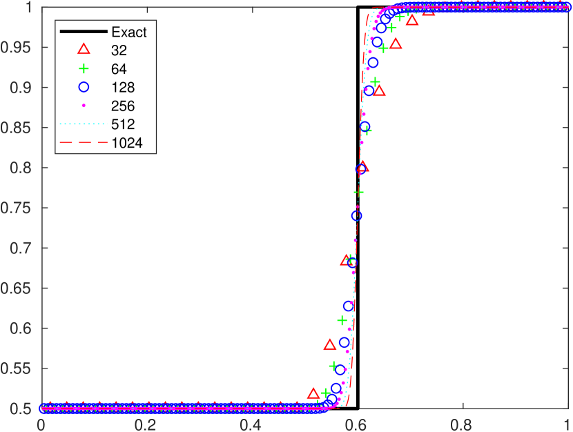
(a) Godunov - Contact

(b) Godunov - Rarefaction

(c) Godunov - Shock

(d) VFV - Contact

(e) VFV - Rarefaction

(f) VFV - Shock

Figure 1: Example 4.1: density $\varrho$ obtained by the Godunov method (top) and the VFV method (bottom).

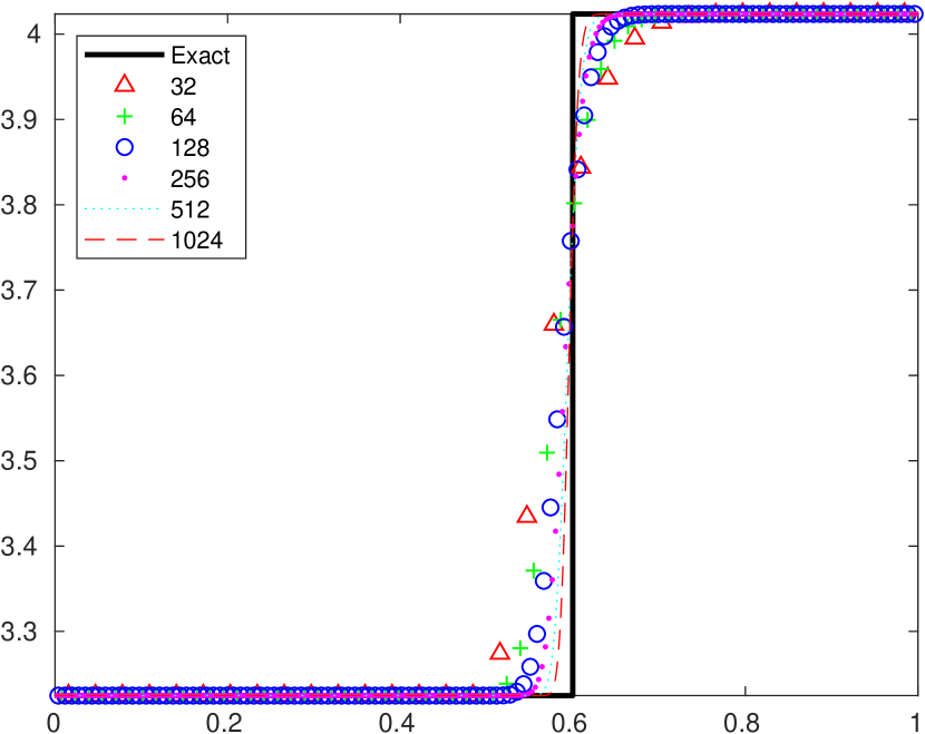
(a) Godunov - Contact

(b) Godunov - Rarefaction

(c) Godunov - Shock

(d) VFV - Contact

(e) VFV - Rarefaction

(f) VFV - Shock

Figure 2: Example 4.1: entropy $\eta$ obtained by the Godunov method (top) and the VFV method (bottom).

(a) Godunov - Contact

(b) Godunov - Rarefaction

(c) Godunov - Shock

(d) VFV - Contact

(e) VFV - Rarefaction

(f) VFV - Shock

Figure 3: Example 4.1: the errors obtained on different meshes.

Table 2: Example 4.1: errors and convergence rates of $\varrho,\eta,\mathbb{E}$ of the Godunov method.

$n=1/h$	Contact		Rarefaction		Shock
	error	order	error	order	error	order
Density
32	0.0569	-	0.0292	-	0.0459	-
64	0.0479	0.2497	0.0201	0.5380	0.0297	0.6252
128	0.0395	0.2753	0.0135	0.5743	0.0224	0.4072
256	0.0332	0.2504	0.0089	0.6098	0.0160	0.4886
512	0.0278	0.2565	0.0057	0.6398	0.0112	0.5183
1024	0.0234	0.2501	0.0036	0.6656	0.0080	0.4805
Entropy
32	0.1038	-	0.0150	-	0.0139	-
64	0.0869	0.2563	0.0105	0.5138	0.0085	0.7083
128	0.0719	0.2732	0.0073	0.5335	0.0054	0.6689
256	0.0603	0.2551	0.0049	0.5524	0.0034	0.6375
512	0.0504	0.2580	0.0033	0.5687	0.0021	0.6807
1024	0.0423	0.2522	0.0022	0.5818	0.0014	0.5978
Relative energy
32	0.069415	-	0.001640	-	0.004126	-
64	0.048272	0.5241	0.000752	1.1246	0.001771	1.2207
128	0.032676	0.5630	0.000330	1.1871	0.000998	0.8274
256	0.022931	0.5109	0.000139	1.2519	0.000504	0.9858
512	0.015997	0.5195	0.000056	1.3075	0.000247	1.0266
1024	0.011269	0.5054	0.000022	1.3554	0.000126	0.9697

Table 3: Example 4.1: errors and convergence rates of $\varrho,\eta,\mathbb{E}$ of the VFV method.

$n=1/h$	Contact		Rarefaction		Shock
	error	order	error	order	error	order
Density
32	0.0751	-	0.0440	-	0.0575	-
64	0.0619	0.2784	0.0307	0.5185	0.0391	0.5584
128	0.0507	0.2877	0.0205	0.5805	0.0268	0.5440
256	0.0418	0.2784	0.0131	0.6479	0.0178	0.5882
512	0.0345	0.2799	0.0081	0.7021	0.0120	0.5752
1024	0.0285	0.2759	0.0048	0.7436	0.0082	0.5465
Entropy
32	0.1356	-	0.0270	-	0.0214	-
64	0.1117	0.2791	0.0182	0.5696	0.0124	0.7956
128	0.0916	0.2862	0.0120	0.6043	0.0068	0.8582
256	0.0755	0.2792	0.0077	0.6295	0.0037	0.8719
512	0.0622	0.2799	0.0049	0.6510	0.0020	0.8713
1024	0.0513	0.2764	0.0031	0.6675	0.0011	0.8287
Relative energy
32	0.116107	-	0.004119	-	0.006390	-
64	0.078778	0.5596	0.001906	1.1118	0.003002	1.0899
128	0.052828	0.5765	0.000818	1.2196	0.001409	1.0911
256	0.035875	0.5583	0.000327	1.3248	0.000613	1.2011
512	0.024321	0.5608	0.000122	1.4157	0.000271	1.1768
1024	0.016577	0.5530	0.000044	1.4865	0.000123	1.1391

Example 4.3.

This experiment is used to further test our theoretical analysis. It describes left-going and right-going rarefaction waves, whose initial data are given by

$$(\varrho,u,p)(x,0)\;=\;\begin{cases}(1,\,-2,\,0.4),&x<0.5,\\ (1,\,2,\,0.4),&x>0.5.\end{cases}$$

Figure 4(a) and (c) show the density $\varrho$ obtained at $T=0.15$ by the Godunov method and the VFV method, respectively. Moreover, the corresponding $L^{2}$-error of $(\varrho,{\bf m},\eta)$ as well as the $L^{1}$-norm of $\mathbb{E}$ are shown in Figure  4(b) and (d), see also Table 4.

Our numerical results show that the converge rate is approximately $1/2$ (resp. $1$) for $(\varrho,{\bf m},\eta)$ (resp. $\mathbb{E}$), which is consistent with our theoretical analysis.

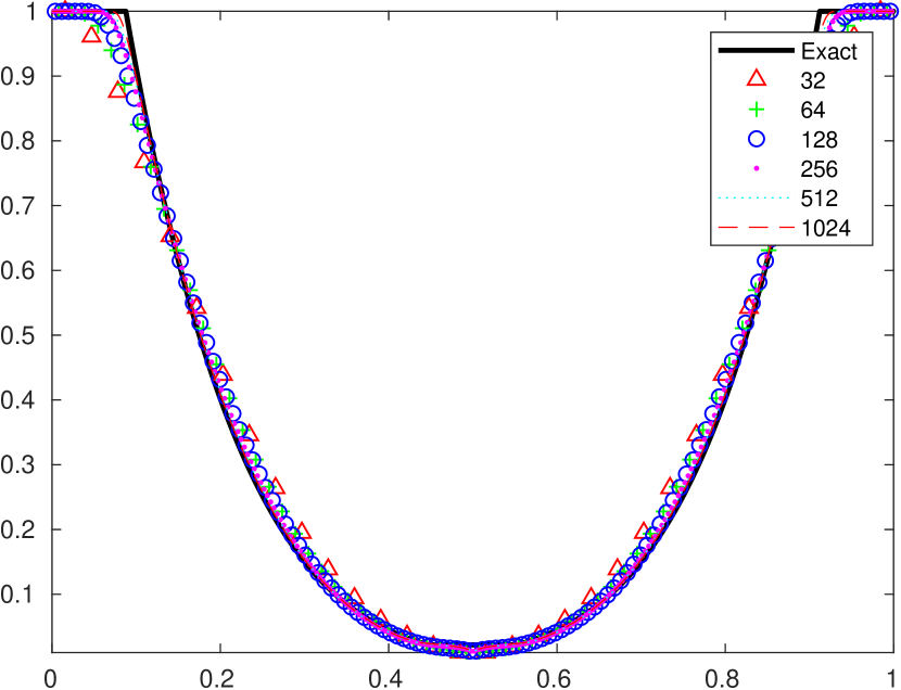
(a) Godunov - $\varrho$

(b) Godunov - error

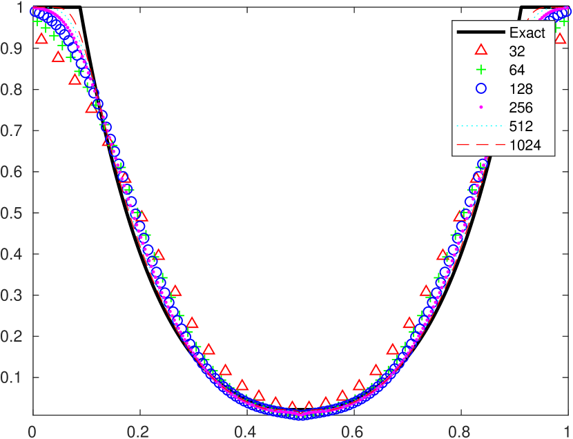
(c) VFV - $\varrho$

(d) VFV - error

Figure 4: Example 4.3: density $\varrho$ and errors at $T=0.15$ of the Godunov method and the VFV method.

Table 4: Example 4.3: errors and convergence rates of $\varrho,{\bf m},\eta,\mathbb{E}$ of the Godunov and VFV methods.

$n$	density		momentum		entropy		relative energy
	error	order	error	order	error	order	error	order
Godunov
32	0.0523	-	0.1299	-	0.1271	-	0.008792	-
64	0.0346	0.5987	0.0869	0.5803	0.0864	0.5566	0.003810	1.2064
128	0.0230	0.5865	0.0579	0.5853	0.0605	0.5135	0.001641	1.2148
256	0.0152	0.6012	0.0380	0.6090	0.0418	0.5354	0.000706	1.2162
512	0.0098	0.6303	0.0244	0.6392	0.0280	0.5755	0.000305	1.2101
1024	0.0062	0.6531	0.0153	0.6671	0.0186	0.5944	0.000134	1.1928
VFV
32	0.1019	-	0.2310	-	0.3146	-	0.047945	-
64	0.0639	0.6723	0.1602	0.5279	0.1824	0.7866	0.019004	1.3350
128	0.0433	0.5616	0.1126	0.5091	0.1153	0.6617	0.007298	1.3808
256	0.0307	0.4950	0.0792	0.5072	0.0807	0.5151	0.002798	1.3830
512	0.0213	0.5301	0.0543	0.5453	0.0560	0.5261	0.001086	1.3660
1024	0.0142	0.5878	0.0361	0.5904	0.0373	0.5884	0.000427	1.3453

Example 4.4.

This experiment is devoted to the 1D Sod problem, in order to test the convergence rate for the solution consisting of the left rarefaction, contact and right shock waves. Although the exact solution is not smooth we can still test corresponding convergence rates. In this example the final time is set to $T=0.15$ and the initial data are given by

$$(\varrho,u,p)(x,0)\;=\;\begin{cases}(1,\,0,\,1),&x<0.5,\\ (0.125,\,0,\,0.1),&x>0.5.\end{cases}$$

Figure 5(a) and (c) show the density obtained with the Godunov and VFV methods on different meshes. Moreover, errors of $(\varrho,{\bf m},\eta)$ and $\mathbb{E}$ are shown in Figure 5(b) and (d), respectively, see also Table 5 for more details.

These numerical results indicate that the convergence rates of $(\varrho,{\bf m},\eta)$ (resp. $\mathbb{E}$) seem to be between $1/4$ and $1/2$ (resp. between $1/2$ and $1$).

(a) Godunov - $\varrho$

(b) Godunov - error

(c) VFV - $\varrho$

(d) VFV - error

Figure 5: Example 4.4: density $\varrho$ and errors obtained on different meshes.

Table 5: Example 4.4: errors and convergence rates of $\varrho,{\bf m},\eta,\mathbb{E}$ of the Godunov and VFV methods.

$n$	density		momentum		entropy		relative energy
	error	order	error	order	error	order	error	order
Godunov
32	0.0378	-	0.0376	-	0.0615	-	0.005135	-
64	0.0273	0.4693	0.0269	0.4819	0.0484	0.3481	0.002642	0.9587
128	0.0203	0.4260	0.0206	0.3855	0.0400	0.2735	0.001561	0.7594
256	0.0151	0.4268	0.0154	0.4217	0.0328	0.2865	0.000913	0.7741
512	0.0114	0.4025	0.0117	0.4003	0.0268	0.2895	0.000554	0.7202
1024	0.0088	0.3773	0.0087	0.4153	0.0221	0.2831	0.000342	0.6978
VFV
32	0.0491	-	0.0525	-	0.0929	-	0.010427	-
64	0.0381	0.3658	0.0377	0.4779	0.0703	0.4023	0.005392	0.9514
128	0.0285	0.4183	0.0270	0.4802	0.0546	0.3641	0.002844	0.9231
256	0.0205	0.4774	0.0192	0.4958	0.0430	0.3441	0.001514	0.9090
512	0.0148	0.4650	0.0140	0.4524	0.0343	0.3274	0.000859	0.8176
1024	0.0110	0.4293	0.0104	0.4337	0.0276	0.3153	0.000508	0.7595

4.2 Two dimensional experiments

In this section we present four two-dimensional Riemann problems. The computational domain is taken as $[0,1]^{2}$. Here the exact solution $\widetilde{{\bf U}}$ used in the relative energy is taken as the reference solution computed on the uniform mesh of $4096^{2}$ cells.

Example 4.5.

The first 2D Riemann problem describes the interaction of four rarefaction waves. The initial data are given by

$$(\varrho,u,v,p)(x,0)\;=\;\begin{cases}(1,\,0,\,0,\,1),&x>0.5,\,y>0.5,\\ (0.5197,\,-0.7259,\,0,\,0.4),&x<0.5,\,y>0.5,\\ (1,\,-0.7259,\,-0.7259,\,1),&x<0.5,\,y<0.5,\\ (0.5197,\,0,\,-0.7259,\,0.4),&x>0.5,\,y<0.5.\end{cases}$$

In this example the final time is set to $T=0.2$. Figure 6(a) and (c) show the density $\varrho$ obtained by the Godunov and VFV method on a mesh with $1024^{2}$ cells. Moreover, Figure 6(b) and (d) show the $L^{2}$-errors of $\varrho,{\bf m},\eta$ and $L^{1}$-norm of $\mathbb{E}$ on different meshes, see also Table 6.

The numerical results show that the convergence rates of $\varrho,{\bf m},\eta$ (resp. $\mathbb{E}$) are slightly better than $1/2$ (resp. 1). This may indicate that our rigorous error estimates are suboptimal in the case of finitely many rarefaction waves.

(a) Godunov - $\varrho$

(b) Godunov - error

(c) VFV - $\varrho$

(d) VFV - error

Figure 6: Example 4.5: density on a mesh with $1024^{2}$ cells and errors at $T=0.2$.

Table 6: Example 4.5: errors and convergence rates of $\varrho,{\bf m},\eta,\mathbb{E}$ of the Godunov and VFV methods.

$n$	density		momentum		entropy		relative energy
	error	order	error	order	error	order	error	order
Godunov
16	0.0572	-	0.0749	-	0.0365	-	0.007821	-
32	0.0421	0.4408	0.0549	0.4475	0.0267	0.4482	0.004021	0.9597
64	0.0298	0.4975	0.0390	0.4950	0.0192	0.4808	0.001952	1.0430
128	0.0202	0.5636	0.0265	0.5567	0.0132	0.5354	0.000874	1.1594
256	0.0129	0.6402	0.0171	0.6316	0.0087	0.6026	0.000354	1.3038
512	0.0077	0.7434	0.0103	0.7353	0.0054	0.6973	0.000125	1.5033
VFV
16	0.0751	-	0.0946	-	0.0515	-	0.014156	-
32	0.0541	0.4729	0.0677	0.4823	0.0353	0.5451	0.007097	0.9962
64	0.0375	0.5276	0.0464	0.5454	0.0235	0.5868	0.003257	1.1237
128	0.0247	0.6061	0.0302	0.6195	0.0151	0.6347	0.001354	1.2666
256	0.0152	0.6976	0.0186	0.7026	0.0093	0.6997	0.000504	1.4263
512	0.0087	0.8063	0.0106	0.8093	0.0054	0.7938	0.000163	1.6287

Example 4.6.

The initial data of the second 2D Riemann problem are given by

$$(\varrho,u,v,p)(x,0)=\begin{cases}(0.5,\,0.5,\,-0.5,\,5),&x>0.5,\,y>0.5,\\ (1,\,0.5,\,0.5,\,5),&x<0.5,\,y>0.5,\\ (2,\,-0.5,\,0.5,\,5),&x<0.5,\,y<0.5,\\ (1.5,\,-0.5,\,-0.5,\,5),&x>0.5,\,y<0.5.\end{cases}$$

The exact solution consists of four interacting contact discontinuities yielding vortex sheets with negative signs. We simulate till $T=0.2$. Figure 7(a) and (c) show the density obtained by the Godunov method and the VFV method on a mesh with $1024^{2}$ cells. The $L^{2}$-errors of $(\varrho,{\bf m},\eta)$ as well as the $L^{1}$-norm of $\mathbb{E}$ are shown in Figure 7(b) and (d), see also Table 7.

Numerical results indicate that $(\varrho,{\bf m},\eta)$ converges with the convergence rate about $1/2$ and the convergence rate for $\mathbb{E}$ is approximately $1$. It seems that our theoretical results for the convergence rates obtained for the strong exact solutions practically holds also for some discontinuous (weak) solutions.

(a) Godunov - $\varrho$

(b) Godunov - error

(c) VFV - $\varrho$

(d) VFV - error

Figure 7: Example 4.6: density on a mesh with $1024^{2}$ cells and errors obtained on different meshes.

Table 7: Example 4.6: errors and convergence rates of $\varrho,{\bf m},\eta,\mathbb{E}$ of the Godunov and VFV methods.

$n$	density		momentum		entropy		relative energy
	error	order	error	order	error	order	error	order
Godunov
16	0.1534	-	0.2355	-	0.2045	-	0.311123	-
32	0.1177	0.3816	0.1780	0.4040	0.1599	0.3543	0.187175	0.7331
64	0.0958	0.2979	0.1419	0.3267	0.1283	0.3180	0.122058	0.6168
128	0.0757	0.3390	0.1096	0.3724	0.1012	0.3425	0.075685	0.6895
256	0.0578	0.3903	0.0816	0.4266	0.0773	0.3881	0.043366	0.8034
512	0.0414	0.4792	0.0569	0.5190	0.0556	0.4761	0.021832	0.9901
VFV
16	0.1932	-	0.3048	-	0.2854	-	0.505011	-
32	0.1547	0.3206	0.2380	0.3572	0.2199	0.3760	0.316830	0.6726
64	0.1241	0.3173	0.1861	0.3548	0.1714	0.3601	0.199627	0.6664
128	0.0970	0.3558	0.1422	0.3878	0.1323	0.3737	0.120510	0.7281
256	0.0729	0.4129	0.1051	0.4360	0.0994	0.4115	0.067199	0.8426
512	0.0514	0.5029	0.0731	0.5248	0.0708	0.4910	0.032644	1.0416

Example 4.7.

The initial data of third 2D Riemann problem are given by

$$(\varrho,u,v,p)(x,0)\;=\;\begin{cases}(1.5,\,0,\,0,\,1.5),&x>0.5,\,y>0.5,\\ (0.5323,\,1.206,\,0,\,0.3),&x<0.5,\,y>0.5,\\ (0.138,\,1.206,\,1.206,\,0.029),&x<0.5,\,y<0.5,\\ (0.5323,\,0,\,1.206,\,0.3),&x>0.5,\,y<0.5,\end{cases}$$

which describes the interaction of four shock waves. In this example the final time is set to $T=0.35$. Figure 8 shows the density on a mesh with $1024^{2}$ cells and errors of $(\varrho,{\bf m},\eta)$ and $\mathbb{E}$ obtained on different meshes. Table 8 lists the errors and convergence rate.

From these numerical results we see that $(\varrho,{\bf m},\eta)$ converges with a ratio between $1/4$ and $1/2$ and $\mathbb{E}$ converges to a ratio between $1/2$ and $1$.

(a) Godunov - $\varrho$

(b) Godunov - error

(c) VFV - $\varrho$

(d) VFV - error

Figure 8: Example 4.7: density on a mesh with $1024^{2}$ cells and errors obtained on different meshes.

Table 8: Example 4.7: errors and convergence rates of $\varrho,{\bf m},\eta,\mathbb{E}$ of the Godunov and VFV methods.

$n$	density		momentum		entropy		relative energy
	error	order	error	order	error	order	error	order
Godunov
16	0.1589	-	0.1764	-	0.2013	-	0.061809	-
32	0.1284	0.3077	0.1404	0.3292	0.1639	0.2964	0.038141	0.6965
64	0.0963	0.4160	0.1133	0.3098	0.1337	0.2940	0.022547	0.7584
128	0.0739	0.3806	0.0926	0.2917	0.1078	0.3106	0.014170	0.6701
256	0.0576	0.3590	0.0777	0.2523	0.0867	0.3137	0.009518	0.5740
512	0.0466	0.3084	0.0650	0.2577	0.0734	0.2409	0.006632	0.5212
VFV
16	0.2075	-	0.2018	-	0.2840	-	0.107017	-
32	0.1566	0.4063	0.1765	0.1938	0.2090	0.4420	0.061465	0.8000
64	0.1246	0.3290	0.1471	0.2626	0.1647	0.3441	0.038455	0.6766
128	0.0975	0.3546	0.1168	0.3325	0.1342	0.2957	0.022700	0.7605
256	0.0719	0.4397	0.0912	0.3576	0.1044	0.3614	0.012882	0.8173
512	0.0519	0.4707	0.0706	0.3689	0.0790	0.4018	0.007407	0.7985

Example 4.8.

The initial data of the fourth 2D Riemann problem are given by

$$(\varrho,u,v,p)(x,0)\;=\;\begin{cases}(0.5313,\,0,\,0,\,0.4),&x>0.5,\,y>0.5,\\ (1,\,0.7276,\,0,\,1),&x<0.5,\,y>0.5,\\ (0.8,\,0,\,0,\,1),&x<0.5,\,y<0.5,\\ (1,\,0,\,0.7276,\,1),&x>0.5,\,y<0.5.\end{cases}$$

This experiment describes the interaction of four discontinuities (the left and bottom discontinuities are two contact discontinuities and the top and right are two shock waves). The final time is set to $T=0.25$. Figure 9 shows the density obtained by the Godunov and VFV methods on a mesh with $1024^{2}$ cells, respectively. The $L^{2}$-errors of $\varrho,{\bf m},\eta$, and the $L^{1}$-norm of $\mathbb{E}$ obtained on different meshes are presented in Figure 9 and Table 9.

These numerical results indicate the convergence rate around $1/2$ for the $L^{2}$-errors in $(\varrho,{\bf m},\eta)$ and rates around $1$ for the $L^{1}$-norm in the relative energy $\mathbb{E}$. Similarly as in the previous experiments, it seems that the VFV method converges faster than the Godunov method.

(a) Godunov - $\varrho$

(b) Godunov - error

(c) VFV - $\varrho$

(d) VFV - error

Figure 9: Example 4.8: density on a mesh with $1024^{2}$ cells and errors obtained on different meshes.

Table 9: Example 4.8: errors and convergence rates of $\varrho,{\bf m},\eta,\mathbb{E}$ of the Godunov and VFV methods.

$n$	density		momentum		entropy		relative energy
	error	order	error	order	error	order	error	order
Godunov
16	0.0791	-	0.1351	-	0.0557	-	0.010648	-
32	0.0604	0.3891	0.1055	0.3567	0.0479	0.2184	0.006658	0.6775
64	0.0458	0.4012	0.0821	0.3619	0.0413	0.2134	0.004084	0.7050
128	0.0344	0.4103	0.0643	0.3538	0.0356	0.2145	0.002519	0.6971
256	0.0258	0.4152	0.0507	0.3426	0.0296	0.2664	0.001537	0.7128
512	0.0191	0.4382	0.0391	0.3724	0.0242	0.2932	0.000896	0.7786
VFV
16	0.1013	-	0.1992	-	0.1343	-	0.023507	-
32	0.0764	0.4069	0.1556	0.3559	0.1066	0.3340	0.014532	0.6938
64	0.0559	0.4522	0.1186	0.3921	0.0837	0.3493	0.008488	0.7757
128	0.0404	0.4676	0.0891	0.4126	0.0650	0.3647	0.004795	0.8240
256	0.0293	0.4640	0.0667	0.4174	0.0493	0.3992	0.002630	0.8664
512	0.0207	0.5035	0.0484	0.4632	0.0355	0.4719	0.001340	0.9725

5 Conclusion

In this paper we have analyzed a priori errors between numerical solutions obtained by the Godunov method and the strong exact solution for the multidimensional Euler system via the relative energy. Assuming that there exist a uniform lower bound on the density and an upper bound on the energy, we showed that the $L^{1}$-norm of the relative energy is equivalent to the $L^{2}$-norm of errors of the numerical solutions, see (2.16). Recalling the consistency formulation proved in [16] and applying Gronwall’s lemma, we have derived the estimates for the relative energy in Theorem 3.1. Specifically, the relative energy converges at least at the rate of $1/2$ in the $L^{1}$-norm. At the same time, the density, momentum and entropy converge at least at the rate of $1/4$ in the $L^{2}$-norm. Being inspired by the fact that the Godunov method for scalar conservation laws has bounded total variations we have formulated additional hypothesis (3.8). If we assume that (3.8) holds, the convergence rate of density, momentum and entropy (resp. relative energy) can be improved to at least $1/2$ (resp. $1$), see Theorem 3.3. Finally, we pointed out that our theoretical analysis rigorously holds only for strong solutions, e.g. for a solution that contains finitely many rarefaction waves.

We have experimentally computed convergence rates for several one- and two-dimensional Riemann problems. From Example 4.1 and Example 4.3 containing only rarefaction waves, we observed that the convergence rate of density, momentum and entropy (resp. relative energy) is slightly higher than $1/2$ (resp. $1$), which is consistent with the theoretical results presented in Theorem 3.3. Our numerical experiments for the Riemann problems with discontinuous solutions show that the convergence rate of the Godunov method are about $1/4$ for the contact wave and about $1/2$ for the shock wave. In future it will be interesting to analyze theoretically the convergence rates towards a weak exact solution containing shock and contact wave.

Funding

M.L. has been funded by the Deutsche Forschungsgemeinschaft (DFG, German Research Foundation) - Project number 233630050 - TRR 146 as well as by TRR 165 Waves to Weather. She is grateful to the Gutenberg Research College for supporting her research.

The research of B.S. leading to these results has received funding from the Czech Sciences Foundation (GAČR), Grant Agreement 21-02411S. The Institute of Mathematics of the Academy of Sciences of the Czech Republic is supported by RVO:67985840.

The research of Y. Y. was funded by Sino-German (CSC-DAAD) Postdoc Scholarship Program in 2020 - Project number 57531629.

Availability of data and materials

The datasets supporting the conclusions of this article are included within the article.

References

- [1] J. Březina and E. Feireisl. Measure-valued solutions to the complete Euler system. J. Math. Soc. Japan, 70(4):1227 - 1245, 2018.
- [2] B. Cockburn, F. Coquel, and P. G. LeFloch. An error estimate for finite volume methods for multidimensional conservation laws. Math. Comp., 63(207):77-103, 1994.
- [3] C. M. Dafermos. The second law of thermodynamics and stability. Arch. Ration. Mech. Anal., 70(2):167-179, 1979.
- [4] E. Feireisl, R. Hošek, D. Maltese, and A. Novotnỳ. Unconditional convergence and error estimates for bounded numerical solutions of the barotropic Navier-Stokes system. Numer. Methods Partial Differential Equations, 33(4):1208-1223, 2017.
- [5] E. Feireisl, M. Lukáčová-Medvid’ová, and H. Mizerová. A finite volume scheme for the Euler system inspired by the two velocities approach. Numer. Math., 144(1):89-132, 2020.
- [6] E. Feireisl, M. Lukáčová-Medvid’ová, and H. Mizerová. Convergence of finite volume schemes for the Euler Equations via dissipative measure-valued solutions. Found. Comput. Math., 20(4):923-966, 2020.
- [7] E. Feireisl, M. Lukáčová-Medvid’ová, H. Mizerová and B. She. Numerical analysis of compressible fluid flows. Volume 20 of MS&A series, Springer-Verlag, 2021.
- [8] E. Feireisl, M. Lukáčová-Medvid’ová, Š. Nečasová, A. Novotný, and B. She. Asymptotic preserving error estimates for numerical solutions of compressible Navier-Stokes equations in the low Mach number regime. Multiscale Modeling & Simulation, 16(1):150-183, 2018.
- [9] E. Feireisl and A. Novotný. Singular limits in thermodynamics of viscous fluids, Second edition. Birkhäuser/Springer, Cham, 2017.
- [10] M. Feistauer, J. Felcman, and I. Straškraba. Mathematical and computational methods for compressible flow. Oxford University Press, 2003.
- [11] S. K. Godunov. A difference method for numerical calculation of discontinuous solutions of the equations of hydrodynamics. Mat. Sb. (N.S.), 47(89):271-306, 1959.
- [12] V. Jovanović and Ch. Rohde. Error estimates for finite volume approximations of classical solutions for nonlinear systems of hyperbolic balance laws. SIAM J. Numer. Anal., 43(6):2423-2449, 2006.
- [13] N. N. Kuznetsov. Accuracy of some approximate methods for computing the weak solutions of a first-order quasi-linear equation. USSR Comput. Math. Math. Phys., 16:105-119, 1976.
- [14] R. J. LeVeque. Numerical methods for conservation laws, volume 132. Springer, 1992.
- [15] J. Li, T. Zhang, and S. Yang. The two-dimensional Riemann problem in gas dynamics, volume 98. CRC Press, 1998.
- [16] M. Lukáčová-Medvid’ová and Y. Yuan. Convergence of first-order finite volume method based on exact Riemann solver for the complete compressible Euler equations. arXiv:2105.02165, 2021.
- [17] H. Mizerová and B. She. Convergence and error estimates for a finite difference scheme for the multi-dimensional compressible Navier-Stokes system. J. Sci. Comput., 84(1):25, 2020.
- [18] C.-W. Shu and S. Osher. Efficient implementation of essentially non-oscillatory shock-capturing schemes. J. Comput. Phys., 77(2):439-471, 1988.
- [19] E. Tadmor and T. Tang. Pointwise error estimates for scalar conservation laws with piecewise smooth solutions. SIAM J. Numer. Anal., 36(6):1739-1758, 1999.
- [20] T. Tang and Z.-H. Teng. The sharpness of Kuznetsov’s -error estimate for monotone difference schemes. Math. Comp., 64(210):581-589, 1995.
- [21] T. Tang and Z.-H. Teng. Viscosity methods for piecewise smooth solutions to scalar conservation laws. Math. Comp., 66(218):495-526, 1997.
- [22] Z.-H. Teng and P. Zhang. Optimal -rate of convergence for the viscosity method and monotone scheme to piecewise constant solutions with shocks. SIAM J. Numer. Anal., 34(3):959-978, 1997.
- [23] E. F. Toro. Riemann solvers and numerical methods for fluid dynamics. A practical introduction. Third edition. Springer-Verlag, Berlin, 2009. xxiv+724 pp.
- [24] J.P. Vila. Convergence and error estimates in finite volume schemes for general multidimensional scalar conservation laws. I. explicite monotone schemes. ESAIM: Math. Model. Numer. Anal., 28(3):267-295, 1994.