Incremental Meta-Learning via Episodic Replay Distillation
for Few-Shot Image Recognition

Abstract

Most meta-learning approaches assume the existence of a very large set of labeled data available for episodic meta-learning of base knowledge. This contrasts with the more realistic continual learning paradigm in which data arrives incrementally in the form of tasks containing disjoint classes. In this paper we consider this problem of Incremental Meta-Learning (IML) in which classes are presented incrementally in discrete tasks. We propose an approach to IML, which we call Episodic Replay Distillation (ERD), that mixes classes from the current task with class exemplars from previous tasks when sampling episodes for meta-learning. These episodes are then used for knowledge distillation to minimize catastrophic forgetting. Experiments on four datasets demonstrate that ERD surpasses the state-of-the-art. In particular, on the more challenging one-shot, long task sequence incremental meta-learning scenarios, we reduce the gap between IML and the joint-training upper bound from 3.5% / 10.1% / 13.4% with the current state-of-the-art to 2.6% / 2.9% / 5.0% with our method on Tiered-ImageNet / Mini-ImageNet / CIFAR100, respectively.

Introduction

Meta-learning, also commonly referred to as “learning to learn”, is a learning paradigm in which a model gains experience over a sequence of learning episodes. This experience is optimized so as to improve the model’s future learning performance on unseen tasks (Hospedales et al. 2021). Meta-learning is one of the most promising techniques to learning models that can flexibly generalize, like humans, to new tasks and environments not seen during training. This capability is generally considered to be crucial for future AI systems. Few-shot learning has emerged as the paradigm-of-choice to test and evaluate meta-learning algorithms. It aims to learn from very limited numbers of samples (as few as just one), and meta-learning applied to few-shot image recognition in particular has attracted increased attention in recent years (Su, Maji, and Hariharan 2020; Bateni et al. 2020; Li et al. 2020; Yang, Liu, and Xu 2021).

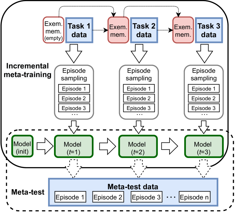
Figure 1: Incremental Meta-Learning (IML) with optional exemplar memories. Data from the previous tasks, unless in exemplar buffer, is unavailable in successive ones. Conventional meta-learning assumes a large number of base classes available for episodic training, while Incremental Meta-Learning requires the meta-learner to update incrementally when a new set of classes (a new task) arrives.

However, most few-shot learning methods are limited in their learning modes: they must train with a large number of classes, with a large number of samples per class, and then to generalize and recognize new classes from few samples. This can lead to poor performance in practical incremental learning situations where the training tasks arrive continually and there are insufficient categories at any given time to learn a performant and general meta-model. The study of learning from data that arrives in such a sequential manner is called continual or incremental learning (De Lange et al. 2021; Schwarz et al. 2018). Catastrophic forgetting is the main challenge of incremental learning systems (McCloskey and Cohen 1989). To address both the challenges of incremental and meta learning, Incremental Meta-Learning (IML, illustrated in Fig. 1) was recently proposed as a way of applying few-shot learning in such incremental learning scenarios (Liu et al. 2020a).

To address the IML problem, Liu et al. (2020a) propose the Indirect Discriminant Alignment (IDA) method. In this method, class centers from previous tasks are represented by anchors which are used to align (by means of a distillation process) the old and new discriminants. They show that this greatly reduces forgetting for short sequences of tasks. They also extended IDA with exemplars (EIML) from old tasks, but surprisingly results showed that this fails to outperform IDA without exemplars. This seems counter-intuitive, since exemplars usually boost performance in incremental learning. We identify the following drawbacks of IDA and EIML: (i) in IDA the anchors are fixed after obtaining them from their corresponding tasks, while semantic drift will gradually make prediction worse with successive tasks; (ii) in EIML exemplars are used only for distillation and computing class anchors, while they are not mixed with current tasks to make the training more robust; and (iii) evaluation is only performed on short sequences (maximally 3 tasks).

In this paper we propose Episodic Replay Distillation (ERD) to better exploit saved exemplars and achieve significant improvement in IML. ERD first divides episode construction into two parts: the exemplar sub-episodes containing only exemplars from past tasks, and the cross-task sub-episodes containing a mixture of previous task exemplars and current task data. Exemplar sub-episodes are then used to produce episode-level classifiers for distillation over the query set. Cross-task sub-episodes combine previous task exemplars with current task samples using a sampling probability $P$. Since the current task contains more samples, and thus higher diversity, a lower $P$ makes better use of the previous and the current samples – an interesting departure from conventional continual learning in which we would typically desire more replay from past tasks.

The main contributions of this paper are:

• Cross-task episodic training: with our proposed cross-task sub-episodes, in which the previous task exemplars and current task samples are mixed to work together to update the meta-learner.

• Episodic replay distillation: different from EIML, our episodic replay distillation is on the episode level and not on class anchors, which in EIML are recomputed with all saved class exemplars.

• State-of-the-art results on all benchmarks: ERD outperforms the state-of-the-art using both Prototypical Networks and Relation Networks. We are also the first to evaluate on long sequences of incremental meta-tasks.

Related work

Few-shot learning

Few-shot learning can be categorized into three main classes of approaches: data augmentation, model enhancement and algorithm-based methods (Wang et al. 2020). Among them, few-shot learning based on metrics or optimization-based approaches are the main directions of current research.

Metric-based methods.  These approaches use embeddings learned from other tasks as prior knowledge to constrain the hypothesis space. Since samples are projected into an embedding subspace, the similar and dissimilar samples can be easily discriminated. Among these techniques, ProtoNets (Snell, Swersky, and Zemel 2017) and RelationNets (Sung et al. 2018) are the most popular.

Optimization-based methods.  These use prior knowledge to search for the model parameters which best approximate the hypothesis in search space and use prior knowledge to alter the search strategy by providing good initialization. Representative methods are MAML (Finn, Abbeel, and Levine 2017) and Reptile (Nichol, Achiam, and Schulman 2018).

Continual learning

Continual learning methods can be divided into three main categories (De Lange et al. 2021): replay-based, regularization-based and parameter-isolation methods. We discuss the first two categories since they are most relevant.

Replay methods.  These prevent forgetting by incorporating data (real or synthetic) from previous tasks. There are two main strategies: exemplar rehearsal (Wu et al. 2019; Hou et al. 2019), which store a small number of training samples (called exemplars) from previous tasks, and pseudo-rehearsal (Hayes et al. 2020; Wu et al. 2018), use generative models learned from previous task data distributions to synthesize data. The classification model in continual learning is a joint classifier and exemplars are used to correct the bias or regularize the gradients. However, in IML there is no joint classifier (only a temporary classifier for each episode). Thus, exemplar-based continual learning methods require adaptation to be applicable to IML: replay for IML should be at the episode level instead of the image level.

Regularization-based methods.  These approaches add a regularization term to the loss function which impedes changes to parameters deemed relevant to previous tasks (Li and Hoiem 2017; Kirkpatrick et al. 2017). Knowledge distillation is popular in continual learning, which aims to either align the outputs at the feature level (Liu et al. 2020b) or the predicted probabilities after a softmax layer (Li and Hoiem 2017). However, aligning at the feature level has been shown to be ineffective (Liu et al. 2020a) and the lack of a unified classifier makes it impossible to align probabilities. Thus, we propose to adapt knowledge distillation to the IML setup.

Meta-learning for continual learning

In addition to the IML setting, there are a few continual learning works that exploit meta-learning, such as La-MAML (Gupta, Yadav, and Paull 2020) and OSAKA (Caccia et al. 2020). These methods focus on improving model performance on task-agnostic incremental classification. There are also some works focusing on dynamic, few-shot visual recognition systems, which aim to learn novel categories from only a few training samples while at the same time not forgetting the base categories (Gidaris and Komodakis 2018; Yoon et al. 2020). Another related setting is FSCIL (Tao et al. 2020), where the authors constrain the continual learning tasks using a few labeled samples.

Different from all these variants, the IML setting casts attention on the original intention of few-shot learning: to make the model generalize to unseen tasks even when training over incremental tasks. Since the seen classes are increasing, the model should gain more generalization ability instead of over-fitting to the current task.

Methodology

In this section, we first define the standard few-shot learning and introduce the incremental meta-learning (IML) setup. Then we describe our approach to IML.

Few-shot and meta-learning

After introducing conventional few-shot learning, we then describe the incremental meta-learning approach.

Conventional few-shot learning.  An approach to standard, non-incremental classification is to learn a parametric approximation $p(y|x;\theta)$ of the posterior distribution of the class $y$ given the input $x$. Such models are trained by minimizing a loss function over a dataset $D$ (e.g. the empirical risk). Few-shot learning, however, presents extra difficulties since the number of samples available for each class $y$ is very small (as few as one). In the meta-learning paradigm, training is divided into two phases: meta-training, in which the model learns how to learn few-shot recognition, and meta-testing where the meta-trained model is evaluated on unseen few-shot recognition tasks.

Meta-training for few-shot learning consists of $T$ episodes (meta-training task in few-shot learning terminology), where each episode $D^{\tau}$ is drawn from the train split of the entire dataset. Few-shot recognition problems consisting of $N$ classes with $K$ training samples per class are referred to $N$-way, $K$-shot recognition problems. Each episode is divided into support set $S$ and query set $Q$: $D^{\tau}=(S,Q)$, where $S=\{(x_{i},y_{i})\}_{i=1}^{NK}$ consists of $N$ training classes each with $K$ images, and $Q=\{(\hat{x}_{i},\hat{y}_{i})\}_{i=1}^{NK^{Q}}$ is a set of $K^{Q}$ images for each of the $N$ selected classes in the episode.

More specifically, we formulate our method based on ProtoNets in this section, and discuss its extension to Relation Networks later. ProtoNets consist of an embedding module $f_{\theta}$ and a classifier module $g$. First, the support set ${S}$ is fed into the embedding module $f_{\theta}$ to obtain class prototypes $\mathbf{c}_{k}$:

$$\mathbf{c}_{k}=\frac{1}{K}\!\!\sum_{(x_{i},k)\in S}\!\!f_{\theta}(x_{i}).$$ (1)

Then, an episode-specific classifier is applied to the query set, where the prediction for class $k$ of query image $\hat{x}$ is:

$$g_{k}(f_{\theta}(S),f_{\theta}(\hat{x}))=p({y}=k|\hat{x};\theta)=\frac{\exp(-d(f_{\theta}(\hat{x}),\mathbf{c}_{k}))}{\sum_{k^{\prime}}\exp(-d(f_{\theta}(\hat{x}),\mathbf{c}_{k^{\prime}}))}$$ (2)

where the summation in the denominator is over all classes $k^{\prime}$ in the support set. Then the meta-loss for updating $\theta$ is:

$$L_{meta}(\theta;S,Q)=-\sum_{(\hat{x},\hat{y})\in Q}[\log g_{\hat{y}}(f_{\theta}(S),f_{\theta}(\hat{x}))].$$ (3)

Incremental Meta-Learning (IML).  When performing incremental meta-learning, data arrives as a sequence of disjoint tasks: $T_{M}={X^{b}_{1},...,X^{b}_{t},...,X^{b}_{M}}$, where $M$ denotes the number of tasks , and $b$ the current training set . The aim of IML is to incrementally learn the parameters $\theta_{t}$ for task $t$ from the disjoint tasks:

$$\theta_{t}^{*}=\arg\min_{\theta_{t}}L(\theta_{t};\theta_{t-1},S_{t},Q_{t}),$$ (4)

Depending on whether we store exemplars from previous tasks, the support set $S_{t}$ and query set $Q_{t}$ can be constructed differently using samples in the current task and exemplars from previous tasks. These query and support sets are described in detail in the next section.

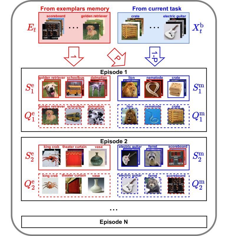
Figure 2: Proposed episode sampling. During episodic meta-learning we build two sets of few-shot problems: exemplar sub-episodes based on only exemplars from previous tasks ($S^{e}_{i}$ and $Q^{e}_{i}$) and cross-task sub-episodes with a mix of exemplars from previous tasks and samples from the current task ($S^{m}_{i}$ and $Q^{m}_{i}$).

Cross-task episodic training

Keeping exemplars from previous tasks is a successful approach to avoid catastrophic forgetting in conventional incremental learning. However, it is not obvious how to leverage exemplars for incremental meta-learning. We propose a novel way of using exemplars for this specific setup.

We consider two strategies for exemplars. The first strategy stores $N_{ex}$ exemplars ($N_{ex}=20$ by default) for each class for each previous task, which is standard in replay-based continual learning methods (UCIR, PODNet, etc.). In this case, the buffer is linearly increased by training sessions. The second strategy fixes the maximum buffer size to $BF$ exemplars ($BF$=1000 by default). We apply both settings in the ablation study and will use the increasing buffer strategy as default.

To fully exploit exemplars from previous tasks, for each episode during meta-learning we construct two sets of support and query images (see Fig. 2). Each episode is broken down into two sets of few-shot problems:

• In each episode we construct a cross-task sub-episode by sampling $N$ classes from the current task with probability $1-P$ and from previous tasks with probability $P$. Thus, we have on average $N*(1-P)$ classes from the current task and $N*P$ from the past. Then, for each class we randomly sample $K$ images as support set $S^{m}$ and $K_{Q}$ images as query set $Q^{m}$ ($m$ denotes that we mix the exemplars with current task samples here).

• We also construct an exemplar sub-episode by sampling $N$ classes from the only the exemplars from previous tasks, each with $K+K_{Q}$ images to form a support set $S^{e}$ and query set $Q^{e}$. Note that this episode is only composed of exemplars from previous tasks.

The reason we sample cross-task sub-episodes with probability $P$ is that exemplars are normally much fewer than samples in the current task, and thus the exemplars are not expected to be as varied as the samples from the current task. With a probability $P$, we can control the balance between current and previous classes in the cross-task sub-episode. And it doesn’t influence the update of the memory buffer.

Given $S^{m},Q^{m}$, the meta-training loss is defined as:

$$L_{meta}(\theta_{t};S^{m},Q^{m})=\sum_{(\hat{x},\hat{y})\in Q^{m}}[-\log g_{\hat{y}}(f_{\theta_{t}}(S^{m}),f_{\theta_{t}}(\hat{x}))].$$ (5)

This loss is only computed over $S^{m}$ and $Q^{m}$ since in $S^{m}$ we have samples from the previous and current tasks.

Episodic Replay Distillation (ERD)

In addition to cross-task episodic training, multiple distillation losses are applied to avoid forgetting when we update the current model (see Fig. 3). We first explore distillation using exemplar sub-episodes. This is computed as:

$$L_{dist}^{e}(\theta_{t};\theta_{t-1},S^{e},Q^{e})=\sum_{\hat{x}\in Q^{e}}\{KL[g(f_{\theta_{t-1}}(S^{e}),f_{\theta_{t-1}}(\hat{x}))$$ (6)

$$||\,g(f_{\theta_{t}}(S^{e}),f_{\theta_{t}}(\hat{x}))]\}$$

where $f_{\theta_{t-1}}$ is the embedding network from the previous task with parameters $\theta_{t-1}$. During training, only the current model $f_{\theta_{t}}$ is updated and $f_{\theta_{t-1}}$ is frozen.

Next, similar to Eq. 6, we also propose a distillation loss using cross-task sub-episodes. It is computed according to:

$$L_{dist}^{m}(\theta_{t};\theta_{t-1},S^{m},Q^{m})=\sum_{\hat{x}\in Q^{m}}\{KL[g(f_{\theta_{t-1}}(S^{m}),f_{\theta_{t-1}}(\hat{x}))$$ (7)

$$||\,g(f_{\theta_{t}}(S^{m}),f_{\theta_{t}}(\hat{x}))]\}$$

The only difference between this distillation loss function and Eq. 6 is the inputs. Finally, $\theta_{t}$ is updated by minimizing:

$$L(\theta_{t};\theta_{t-1},S^{e},Q^{e},S^{m},Q^{m}) =L_{meta}+\lambda_{m}\cdot L_{dist}^{m}+\lambda_{e}\cdot L_{dist}^{e}$$ (8)

$\lambda_{m}$ and $\lambda_{e}$ are trade-off parameters.

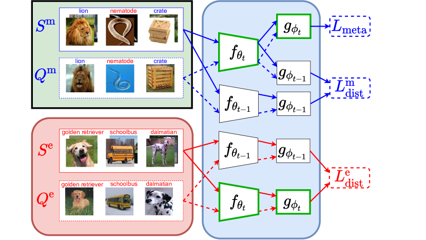
Figure 3: Proposed Episodic Replay Distillation framework. Modules in green are the current embedding model, which are updated with both cross-task and exemplar sub-episodes. Red lines and blue lines are data flows for exemplar sub-episode and cross-task sub-episode, respectively. Solid lines and dotted lines indicate the data flows from support set and query set respectively. When computing loss for ProtoNets, $g$ is a parametric-free operation, while for Relation Networks, $g$ consists of a set of parameters $\phi$.

Extension to Relation Networks

Episodic Replay Distillation is not limited to ProtoNets. It can also be extended to Relation Networks (Sung et al. 2018), which consist of a relation module with parameters $\phi$. Losses introduced in previous sections are adapted as:

$$L_{meta}(\theta_{t},\phi_{t};S^{m},Q^{m}) =$$ (9)

$$\sum_{({x},{y})\in S^{m},(\hat{x},\hat{y})\in Q^{m}} [g_{\phi_{t}}(\mathcal{C}(f_{\theta_{t}}(x),f_{\theta_{t}}(\hat{x})))-\mathbf{1}(y=\hat{y})]^{2},$$

where $\mathcal{C}$ is the concatenation of support set and query set embeddings, $\mathbf{1}$ is the Boolean function returning 1 when its argument is true and 0 otherwise. Distillation losses are updated as (MSE denotes mean squared error):

$$L_{dist}^{m}(\theta_{t},\phi_{t};\theta_{t-1},S^{m},Q^{m}) =$$ (10)

$$\sum_{{x}\in S^{m},\hat{x}\in Q^{m}}\{\mathrm{MSE} [g_{\phi_{t-1}}(\mathcal{C}(f_{\theta_{t-1}}(x),f_{\theta_{t-1}}(\hat{x}))),$$

$$g_{\phi_{t-1}}(\mathcal{C}(f_{\theta_{t}}(x),f_{\theta_{t}}(\hat{x})))]\}$$

$$L_{dist}^{e}(\theta_{t},\phi_{t};\theta_{t-1},\phi_{t-1},S^{e},Q^{e}) =$$

$$\sum_{{x}\in S^{e},\hat{x}\in Q^{e}}\{\mathrm{MSE}[ g_{\phi_{t-1}}(\mathcal{C}(f_{\theta_{t-1}}(x),f_{\theta_{t-1}}(\hat{x}))),$$

$$g_{\phi_{t}}(\mathcal{C}(f_{\theta_{t}}(x),f_{\theta_{t}}(\hat{x})))]\},$$

Although Relation Networks and ProtoNets adopt different ways to calculate the prediction probabilities for given query images, they share similar network architectures with embedding and classification modules. This type of architecture is widely used in metric-based few-shot learning and we believe that our method can be easily adapted to other methods with similar architectures.

Experiments

In this section we report on a range of experiments to quantify the contribution of each element of our proposed approach and to compare our performance against the state-of-the-art in continual few-shot image classification.

Experimental setup

Here we describe the datasets and experimental protocols in our experiments. Source code is in supplementary material.

	IML training tasks				Meta-test Images
Task #:	1	2	…	16
Classes per task:	5	5	…	5	20
Images in train split:	500	500		500	600
Images in test split:	100	100		100

Table 1: Our proposed 16-task split of Mini-ImageNet and CIFAR100 datasets for incremental few-shot learning.

Datasets.  We evaluate performance on four datasets: Mini-ImageNet (Vinyals et al. 2016), CIFAR100 (Krizhevsky 2009), CUB-200-2011 (Wah et al. 2011) and Tiered-ImageNet (Ren et al. 2018). Mini-ImageNet consists of 600 84$\times$84 images from 100 classes. We propose a split with 20 of these classes as meta-test set unseen in all training sessions. The other 80 classes are used to form the incremental meta-training set which is split into 4 or 16 tasks with equal numbers of classes for incremental meta-learning. Each class in each task is then divided into a meta-training split with 500 images, from which support and query sets are sampled for each episode, and a test split with 100 images that is set aside for task-specific evaluation. We select $N_{ex}=20$ exemplars per class before proceeding to the next task. Table 1 is an illustration of the 16-task setting data split.

CIFAR100 also contains 100 classes, each with 600 images, so we use the same splitting criteria as for Mini-ImageNet. The CUB dataset contains 11,788 images of 200 birds species. We split 160 classes into an incremental meta-training set and the other 40 are kept as a meta-test set of unseen classes. We divide the 160 classes into 4 or 16 equal incremental meta-learning tasks. Since there are fewer images per class, we choose $N_{ex}=10$ images per class as exemplars for each previous task and 20 images as test split for each task. On Tiered-ImageNet, We keep the same test split (8 categories, 160 classes) as in the original setup, then split the training and validation classes (26 categories, 448 classes) into 16 equal tasks. And since in this case, each task is with more classes than other datasets setup, it’s a much easier setting, we only test it under the 16-task setup.

Implementation details.  We use ProtoNets as our main meta-learner, but also verify ERD using Relation Networks. We evaluate both the widely used 4-Conv (Snell, Swersky, and Zemel 2017) and ResNet-12 (He et al. 2016) as feature extractors. We sample 200 and 50 episodes for 4-task and 16-task setups per task in each training epoch respectively. We train each meta-learning task for 200 epochs by Adam.

We evaluate on two widely used few-shot setups: 1-shot/5-way and 5-shot/5-way. We include results on both incremental training tasks and the unseen meta-test set. For each task (including the unseen set), we randomly construct $N_{ep}$ episodes to obtain the final performance of the meta-learner, which is computed as the mean and 95% confidence interval of the classification accuracy across $N_{ep}$ episodes. $N_{ep}$ is 10000 for the 4-task and 1000 for the 16-task setup. Here we only report the mean accuracy, but confidence intervals are reported in the supplementary material. For exemplar selection for ProtoNets, we use the Nearest-To-Center (NTC) criterion to select the samples closest to the class-mean. For Relation Networks, since the image embeddings are feature maps instead of feature vectors, we cannot obtain the class prototypes and therefore use random selection. By default, we set $\lambda_{m}=\lambda_{e}=0.5,P=0.2$.

Compared methods.  We compare our method with a finetuning baseline (FT), IDA (Liu et al. 2020a), and a variant of IDA with $N_{ex}$ exemplars per class (EIML). The meta-test upper bounds are obtained by jointly training on all training tasks and testing on the unseen meta-test split (i.e. the standard setting in non-incremental few-shot learning). We evaluate on two sets of tasks separately for comparison. At each training session, we evaluate on previously seen classes as way of measuring forgetting. This we call mean accuracy on seen classes. Performance on the meta-test set (all unseen classes) is to show the generalization ability.

Experiments results

Here we describe the experimental results on long/short task sequences and comparison with continual learning methods. Experiments on long task sequences.  In Fig. 4 we report results on 16-task 1-shot/5-shot 5-way incremental meta-learning for three datasets: CIFAR100, Mini-ImageNet and Tiered-ImageNet (Results on CUB dataset in supplementary). The first and third columns in Fig. 4 show mean accuracy on previous tasks, from which it is obvious that we achieve significantly less forgetting compared to other methods. From the second and fourth columns, the meta-test accuracy for ERD increases with more meta-training tasks due to seeing more diverse classes, while for IDA and EIML, in some training sessions, the performance drops significantly. This might be due to forgetting on previous tasks and overfitting on current task. Notably, for our method the meta-test accuracy after the last task is much closer to the joint training upper bound, which is learned using all training tasks.

Note also that EIML works much better than IDA after about the first 4 tasks. That might be for the same reason that, in the original IDA paper, they report similar results for both IDA and EIML, which is simply due to evaluating on only very short sequences of two or three tasks. This is likely due to anchor drift in IDA and the fact that in EIML exemplars could be used to re-calibrate them. In general, all methods work better in the 5-shot. The underlying reason for this is that the 5-shot is simpler compared to 1-shot.

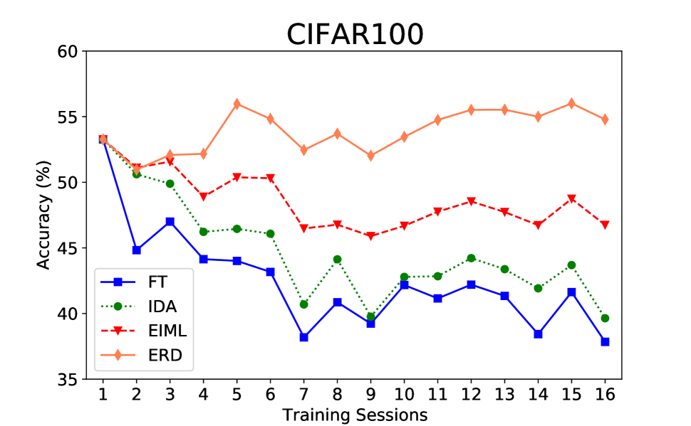
(a) 1-shot mean accuracy on seen

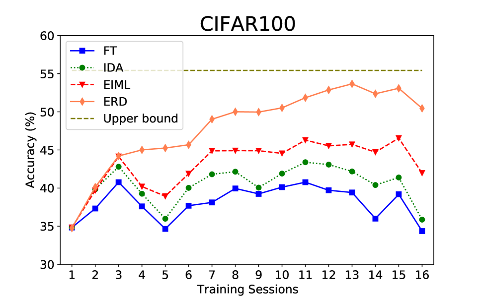
(b) 1-shot meta-test accuracy

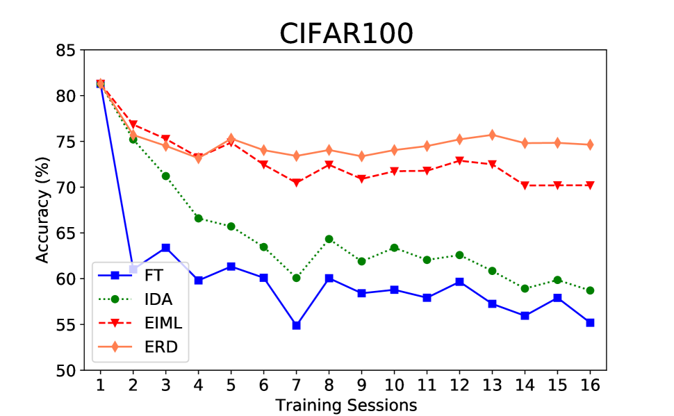
(c) 5-shot mean accuracy on seen

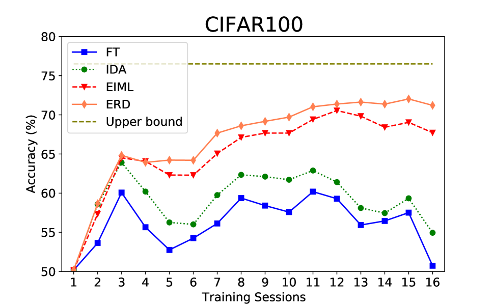
(d) 5-shot meta-test accuracy

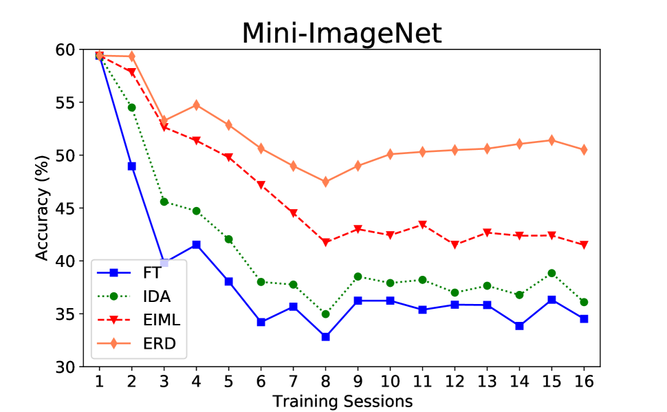
(e) 1-shot mean accuracy on seen

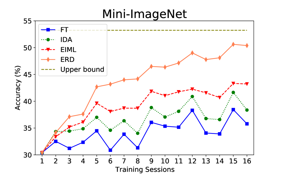
(f) 1-shot meta-test accuracy

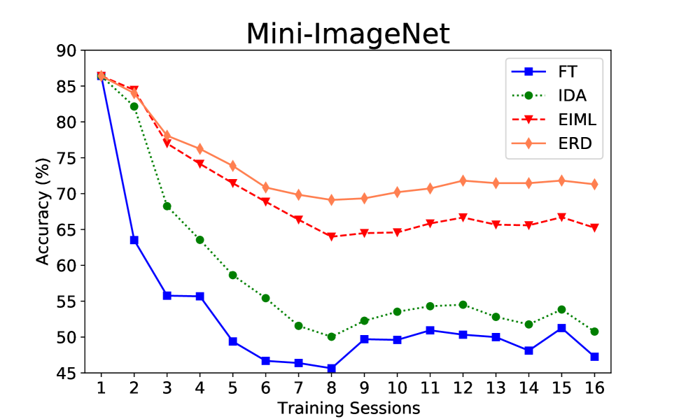
(g) 5-shot mean accuracy on seen

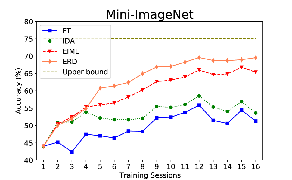
(h) 5-shot meta-test accuracy

(i) 1-shot mean accuracy on seen

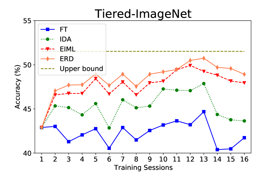
(j) 1-shot meta-test accuracy

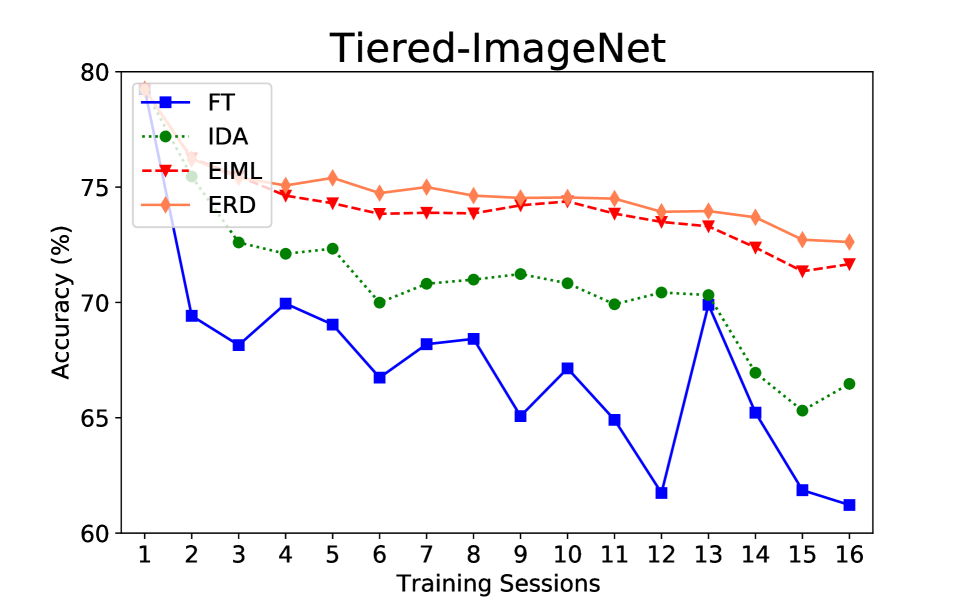
(k) 5-shot mean accuracy on seen

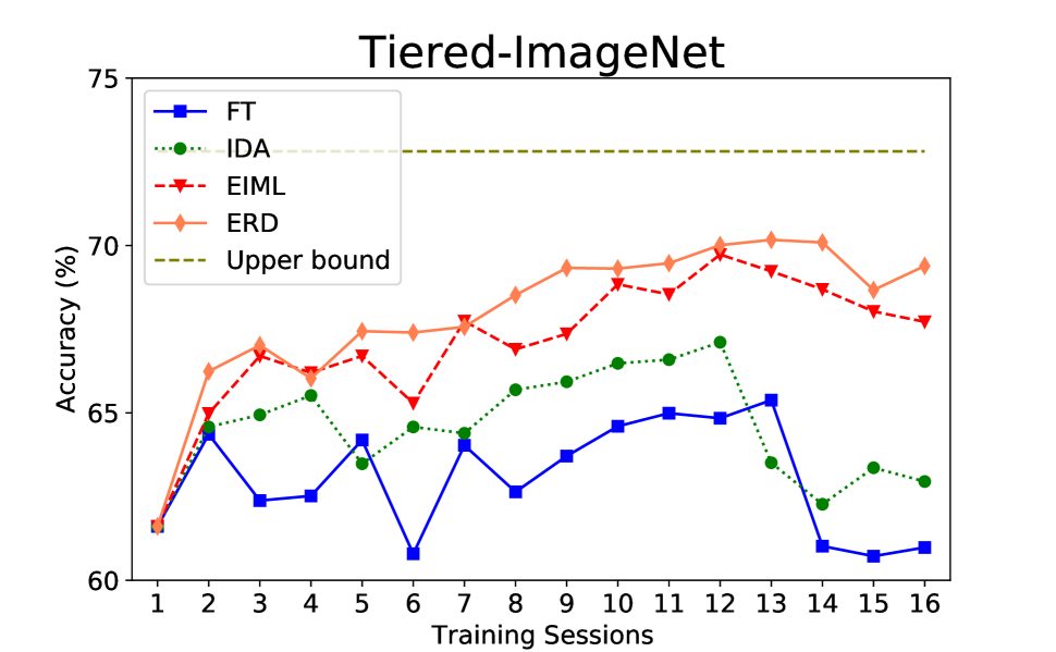
(l) 5-shot meta-test accuracy

Figure 4: Results on the 1- and 5-shot, 5-way 16-task setup with a 4-Conv backbone and ProtoNets meta-learner. Evaluations are on CIFAR100, Mini-ImageNet and Tiered-ImageNet datasets.

Experiments on short task sequences.

Learner:	ProtoNets
Dataset:	Mini-ImageNet				CIFAR100				CUB
Backbone:	4-Conv
	Upper bound: 53.2				Upper bound: 55.4				Upper bound: 61.1
Sessions:	1	2	3	4	1	2	3	4	1	2	3	4
FT	43.8	44.1	42.4	37.9	44.6	45.1	48.0	45.5	45.1	54.6	54.9	58.8
IDA	43.8	48.3	47.2	42.3	44.6	48.0	51.3	47.6	45.1	54.7	54.9	58.7
EIML	43.8	48.8	49.4	47.5	44.6	48.0	52.0	51.7	45.1	53.4	55.0	58.9
ERD	43.8	51.1	52.3	53.0	44.6	49.5	53.6	55.1	45.1	53.9	58.3	60.8
Backbone:	ResNet-12
	Upper bound: 59.9				Upper bound: 61.8				Upper bound: 74.8
Sessions:	1	2	3	4	1	2	3	4	1	2	3	4
FT	45.7	45.9	42.1	37.7	47.0	45.0	51.0	44.6	53.4	64.0	63.7	66.8
IDA	45.7	53.0	53.7	47.6	47.0	53.6	59.2	54.8	53.4	64.4	68.8	73.3
EIML	45.7	53.2	56.5	55.8	47.0	53.3	58.3	57.8	53.4	62.8	69.1	73.3
ERD	45.7	55.2	58.2	59.3	47.0	55.6	61.3	61.4	53.4	66.1	72.4	74.1

Table 2: Meta-test accuracy by training session in the 4-task setting. We evaluate 1-shot and 5-way few-shot recognition on three datasets using two different backbones.

We also compare our method with others on short sequences. In table 2, we first evaluate our model with a 4-Conv backbone on 1-shot/5-way few-shot on three datasets (5-shot results in supplementary). We see that FT suffers from catastrophic forgetting, and meta-test accuracy drops dramatically and exhibits overfitting to the current task. IDA is not able to improve meta-test accuracy on Mini-ImageNet, but improves performance on CIFAR100 and CUB. As for EIML, with exemplars it shows large improvement compared to IDA. However, our method ERD outperforms EIML by a large margin after learning all four tasks. These results further confirm the observations on the 16-task setting. ERD not only achieves the best performance with less forgetting, but also gets closer to the upper bound after the last task. Note also that CIFAR100 and Mini-ImageNet are coarse-grained datasets, compared to CUB, which makes few shot classification much harder due to intra-class variability.

Finally, we consider ResNet-12 as a backbone to show that ERD can be applied to different backbones. Our method achieves consistently better performance over other methods with much higher accuracy than using 4-Conv backbone.

Comparison with standard CL methods.  As shown in Table 3, we compare our method with three state-of-the-art CL methods: iCaRL (Rebuffi et al. 2017), PODNet (Douillard et al. 2020) and UCIR (Hou et al. 2019). For the evaluation on seen classes, we followed the same protocol as IDA, where the average classification accuracy is calculated over $N_{ep}$ episodes. Note that this is different from the evaluation in regular CL. Thus, these methods cannot be directly applied in this scenario. Instead, we use them to continually learn representations and then evaluate them with a nearest centroid classifier for few-shot learning. Observe how, on seen classes evaluation, UCIR works better than iCaRL and PODNet. But under meta-test evaluation, iCaRL works the best among them. PODNet performs similar to the FT baseline in both cases. Clearly, without episodic training, regular CL methods are inferior to our proposed ERD.

Dataset: CIFAR100 , Learner: ProtoNets, Backbone: 4-Conv
Evaluation:	Meta-test accuracy					Mean accuracy on seen classes
Sessions:	2	4	8	16	avg	2	4	8	16	avg
FT	37.3	37.6	40.0	34.4	38.1	44.8	44.1	40.9	37.8	42.5
IDA	39.8	39.3	42.2	35.9	40.3	50.6	46.2	44.1	39.6	44.7
EIML	39.7	40.2	44.9	42.0	43.1	51.1	48.9	46.8	46.7	48.6
ERD	40.1	45.0	50.0	50.5	48.1	51.0	52.2	53.7	54.8	53.9
iCaRL	39.0	42.0	43.4	45.2	43.1	50.1	47.2	46.5	48.0	48.5
UCIR	35.1	36.3	39.5	42.2	39.3	53.6	50.5	50.1	51.9	52.4
PODNet	36.0	37.0	37.1	36.4	37.0	52.9	43.8	41.0	41.1	44.6

Table 3: Meta-test accuracy and mean accuracy on seen classes by training session on the 16-task setting. We evaluate 1-shot/5-way few-shot recognition to compare with continual learning methods (5-shot results in supplementary).

Ablation study

In Fig. 5 we show the ablation study on CIFAR100 under the 16-task 1-shot/5-way setup with 4-Conv as the backbone. We plot meta-test accuracy curves to compare among variants since it is the most important evaluation metric in IML.

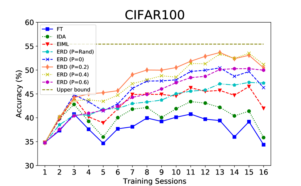
(a) Ablation on $P$

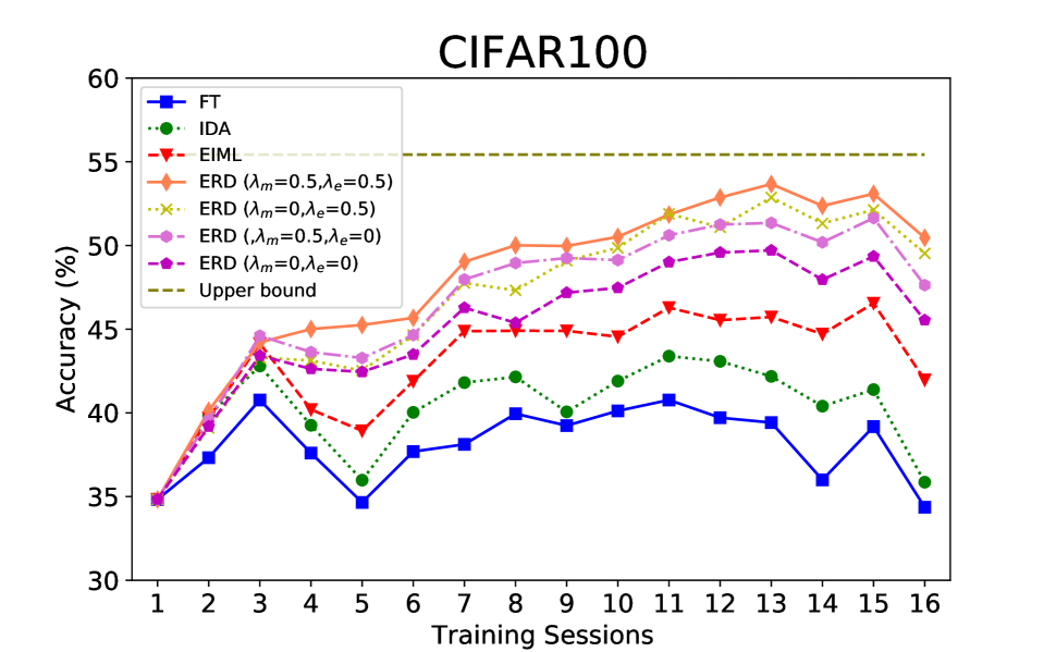
(b) Ablation on $\lambda_{e}$, $\lambda_{m}$

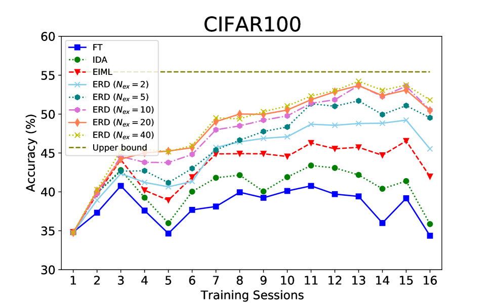
(c) Ablation on $N_{ex}$

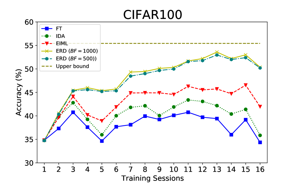
(d) Ablation on $BF$

Figure 5: Ablation study on 16-task 1-shot/5-way setup on CIFAR100 with 4-Conv. We plot the meta-test accuracy to compare.

Ablation on $P$ with $\lambda_{m}=\lambda_{e}=0.5$.  As shown in Fig. 5, ERD obtains the best performance with $P=0.2$. This is what we use by default for all previous experiments. When $P=0$, it means there are no previous classes in the cross-task sub-episode, which performs worse than our variants with higher probabilities, especially with $P=0.2$ and $P=0.4$. As $P$ decreases from 0.6 to 0.2, the performance consistently improves. The reason is that lower $P$ means having more current samples, which can ensure the diversity of training samples. This phenomenon is different from the conventional use of exemplars in incremental learning, where more balanced exemplar sampling is preferable. $P=\mbox{Rand}$ instead means $P$ is not fixed, but that classes in each cross-task sub-episode are randomly selected from all encountered classes up to now and $P$ is increasing with successive tasks. It achieves worse results because there are more and more previous classes with less diverse samples. Most of our variants outperform EIML by a large margin. We keep $P\geq 0.2$ to ensure that at least one previous class occurs in each episode for 5-way few-shot learning.

As a conclusion, the value of $P$ controls the number of previous classes used in the current episode, which is a key component of cross-task episodic training.

Ablation on $\lambda_{m}$ and $\lambda_{e}$ with $P=0.2$.  To understand the role of each distillation component in Eq (8), we ablate the distillation loss terms. As shown in Fig. 5, our method achieves the best with $\lambda_{m}=0.5$ and $\lambda_{e}=0.5$, which indicates both distillation terms playing a crucial role in overcoming forgetting and generalizing to unseen tasks. ERD with $\lambda_{m}=0.5$, $\lambda_{e}=0$ works similarly to ERD with $\lambda_{m}=0$, $\lambda_{e}=0.5$. They both achieve much better performance than without using distillations ($\lambda_{m}=0$ and $\lambda_{e}=0$).

Ablation on memory buffer with $P=0.2,\lambda_{m}=\lambda_{e}=0.5$.  In this experiment, we fix other hyper-parameters to show how different numbers of exemplars affect incremental learning performance. We give ablations on $N_{ex}$ and with bounded buffer size $BF$ which are both commonly used for exemplar rehearsal. From Fig. 5 we see that increasing $N_{ex}$ leads to a noticeable increase in performance going from 2 to 20 exemplars. However, the gain is marginal beyond 20 exemplars per class. From Fig. 5, we can observe that with a smaller bounded buffer with only $BF=500$ exemplars, ERD is still close to the joint training upper bound, showing the importance of proposed sub-episodes.

Extension to Relation Networks

Since in Relation Networks there is no embedding to exploit for computing prototypes as in ProtoNets, IDA and EIML cannot be directly applied. Therefore we only compare with FT in this experiment. As the experimental results shown in Table 4, our model not only surpasses the FT baseline significantly, but also gets close to the joint training upper bounds after the last task, especially on the CUB dataset.

Learner:	Relation Networks
Datasets:	Mini-ImageNet				CIFAR100				CUB
Backbone:	4-Conv				4-Conv				4-Conv
1-shot/5-way 16-task setting
	Upper bound: 52.0				Upper bound: 59.2				Upper bound: 51.6
Sessions:	2	4	8	16	2	4	8	16	2	4	8	16
FT	24.4	28.5	25.5	28.7	31.1	30.0	35.2	26.8	37.1	38.1	37.0	34.0
ERD	27.7	29.9	34.5	30.1	35.6	39.3	45.7	35.9	37.3	42.9	47.9	42.5
1-shot/5-way 4-task setting
	Upper bound: 52.0				Upper bound: 59.2				Upper bound: 51.6
Sessions:	1	2	3	4	1	2	3	4	1	2	3	4
FT	41.70	41.65	38.51	33.33	42.9	45.3	45.7	42.3	45.7	47.9	48.5	50.3
ERD	41.70	45.84	48.35	49.73	42.9	48.2	51.2	51.4	45.7	48.5	49.4	51.4

Table 4: Meta-test accuracy by training sessions on the 4-task and 16-task settings. We evaluate 1-shot/5-way few-shot recognition on Mini-ImageNet, CIFAR-100 and CUB.

Conclusions

In this paper we proposed Episodic Replay Distillation, an approach to incremental few-shot recognition that uses episodic meta-learning over episodes split into cross-task and exemplar sub-episodes. This division into two types of few-shot learning sub-episodes allows us to balance acquisition of new task knowledge with retention of knowledge from previous tasks and thus avoid catastrophic forgetting. Experiments on multiple few-shot learning datasets demonstrate the effectiveness of ERD. Our method is especially effective on long task sequences, where we significantly close the gap between incremental few-shot learning and the joint training upper bound.

Acknowledgments.  We acknowledge the support from Huawei Kirin Solution.

See pages ,- of figs/supp.pdf

References

- Bateni et al. (2020) Bateni, P.; Goyal, R.; Masrani, V.; Wood, F.; and Sigal, L. 2020. Improved few-shot visual classification. In Proceedings of the IEEE Conference on Computer Vision and Pattern Recognition, 14493–14502.
- Caccia et al. (2020) Caccia, M.; Rodriguez, P.; Ostapenko, O.; Normandin, F.; Lin, M.; Caccia, L.; Laradji, I.; Rish, I.; Lacoste, A.; Vazquez, D.; et al. 2020. Online fast adaptation and knowledge accumulation: a new approach to continual learning. In Advances in Neural Information Processing Systems.
- De Lange et al. (2021) De Lange, M.; Aljundi, R.; Masana, M.; Parisot, S.; Jia, X.; Leonardis, A.; Slabaugh, G.; and Tuytelaars, T. 2021. A continual learning survey: Defying forgetting in classification tasks. IEEE Transactions on Pattern Analysis and Machine Intelligence.
- Douillard et al. (2020) Douillard, A.; Cord, M.; Ollion, C.; Robert, T.; and Valle, E. 2020. Podnet: Pooled outputs distillation for small-tasks incremental learning. In European Conference on Computer Vision, 86–102. Springer.
- Finn, Abbeel, and Levine (2017) Finn, C.; Abbeel, P.; and Levine, S. 2017. Model-agnostic meta-learning for fast adaptation of deep networks. In International Conference on Machine Learning, 1126–1135. PMLR.
- Gidaris and Komodakis (2018) Gidaris, S.; and Komodakis, N. 2018. Dynamic few-shot visual learning without forgetting. In Proceedings of the IEEE Conference on Computer Vision and Pattern Recognition, 4367–4375.
- Gupta, Yadav, and Paull (2020) Gupta, G.; Yadav, K.; and Paull, L. 2020. La-MAML: Look-ahead Meta Learning for Continual Learning. In Advances in Neural Information Processing Systems.
- Hayes et al. (2020) Hayes, T. L.; Kafle, K.; Shrestha, R.; Acharya, M.; and Kanan, C. 2020. REMIND Your Neural Network to Prevent Catastrophic Forgetting. In European Conference on Computer Vision.
- He et al. (2016) He, K.; Zhang, X.; Ren, S.; and Sun, J. 2016. Deep residual learning for image recognition. In Proceedings of the IEEE Conference on Computer Vision and Pattern Recognition, 770–778.
- Hospedales et al. (2021) Hospedales, T.; Antoniou, A.; Micaelli, P.; and Storkey, A. 2021. Meta-learning in neural networks: A survey. IEEE Transactions on Pattern Analysis and Machine Intelligence.
- Hou et al. (2019) Hou, S.; Pan, X.; Loy, C. C.; Wang, Z.; and Lin, D. 2019. Learning a unified classifier incrementally via rebalancing. In Proceedings of the IEEE Conference on Computer Vision and Pattern Recognition, 831–839.
- Kirkpatrick et al. (2017) Kirkpatrick, J.; Pascanu, R.; Rabinowitz, N.; Veness, J.; Desjardins, G.; Rusu, A. A.; Milan, K.; Quan, J.; Ramalho, T.; Grabska-Barwinska, A.; et al. 2017. Overcoming catastrophic forgetting in neural networks. Proceedings of the national academy of sciences, 114(13): 3521–3526.
- Krizhevsky (2009) Krizhevsky, A. 2009. Learning multiple layers of features from tiny images.
- Li et al. (2020) Li, K.; Zhang, Y.; Li, K.; and Fu, Y. 2020. Adversarial feature hallucination networks for few-shot learning. In Proceedings of the IEEE Conference on Computer Vision and Pattern Recognition, 13470–13479.
- Li and Hoiem (2017) Li, Z.; and Hoiem, D. 2017. Learning without forgetting. IEEE Transactions on Pattern Analysis and Machine Intelligence, 40(12): 2935–2947.
- Liu et al. (2020a) Liu, Q.; Majumder, O.; Achille, A.; Ravichandran, A.; Bhotika, R.; and Soatto, S. 2020a. Incremental Few-Shot Meta-learning via Indirect Discriminant Alignment. In European Conference on Computer Vision, 685–701. Springer.
- Liu et al. (2020b) Liu, X.; Wu, C.; Menta, M.; Herranz, L.; Raducanu, B.; Bagdanov, A. D.; Jui, S.; and van de Weijer, J. 2020b. Generative Feature Replay For Class-Incremental Learning. In Proceedings of the IEEE/CVF Conference on Computer Vision and Pattern Recognition Workshops, 226–227.
- McCloskey and Cohen (1989) McCloskey, M.; and Cohen, N. J. 1989. Catastrophic interference in connectionist networks: The sequential learning problem. In Psychology of learning and motivation, volume 24. Elsevier.
- Nichol, Achiam, and Schulman (2018) Nichol, A.; Achiam, J.; and Schulman, J. 2018. On first-order meta-learning algorithms. arXiv preprint arXiv:1803.02999.
- Rebuffi et al. (2017) Rebuffi, S.-A.; Kolesnikov, A.; Sperl, G.; and Lampert, C. H. 2017. icarl: Incremental classifier and representation learning. In Proceedings of the IEEE Conference on Computer Vision and Pattern Recognition, 2001–2010.
- Ren et al. (2018) Ren, M.; Triantafillou, E.; Ravi, S.; Snell, J.; Swersky, K.; Tenenbaum, J. B.; Larochelle, H.; and Zemel, R. S. 2018. Meta-learning for semi-supervised few-shot classification. International Conference on Learning Representations.
- Schwarz et al. (2018) Schwarz, J.; Luketina, J.; Czarnecki, W. M.; Grabska-Barwinska, A.; Teh, Y. W.; Pascanu, R.; and Hadsell, R. 2018. Progress & compress: A scalable framework for continual learning. In International Conference on Machine Learning.
- Snell, Swersky, and Zemel (2017) Snell, J.; Swersky, K.; and Zemel, R. S. 2017. Prototypical networks for few-shot learning. Advances in Neural Information Processing Systems.
- Su, Maji, and Hariharan (2020) Su, J.-C.; Maji, S.; and Hariharan, B. 2020. When does self-supervision improve few-shot learning? In European Conference on Computer Vision, 645–666. Springer.
- Sung et al. (2018) Sung, F.; Yang, Y.; Zhang, L.; Xiang, T.; Torr, P. H.; and Hospedales, T. M. 2018. Learning to compare: Relation network for few-shot learning. In Proceedings of the IEEE Conference on Computer Vision and Pattern Recognition, 1199–1208.
- Tao et al. (2020) Tao, X.; Hong, X.; Chang, X.; Dong, S.; Wei, X.; and Gong, Y. 2020. Few-shot class-incremental learning. In Proceedings of the IEEE Conference on Computer Vision and Pattern Recognition, 12183–12192.
- Vinyals et al. (2016) Vinyals, O.; Blundell, C.; Lillicrap, T.; Kavukcuoglu, K.; and Wierstra, D. 2016. Matching networks for one shot learning. Advances in Neural Information Processing Systems.
- Wah et al. (2011) Wah, C.; Branson, S.; Welinder, P.; Perona, P.; and Belongie, S. 2011. The Caltech-UCSD Birds-200-2011 Dataset. Technical Report CNS-TR-2011-001, California Institute of Technology.
- Wang et al. (2020) Wang, Y.; Yao, Q.; Kwok, J. T.; and Ni, L. M. 2020. Generalizing from a few examples: A survey on few-shot learning. ACM Computing Surveys (CSUR), 53(3): 1–34.
- Wu et al. (2018) Wu, C.; Herranz, L.; Liu, X.; van de Weijer, J.; Raducanu, B.; et al. 2018. Memory replay gans: Learning to generate new categories without forgetting. Advances in Neural Information Processing Systems, 31: 5962–5972.
- Wu et al. (2019) Wu, Y.; Chen, Y.; Wang, L.; Ye, Y.; Liu, Z.; Guo, Y.; and Fu, Y. 2019. Large scale incremental learning. In Proceedings of the IEEE Conference on Computer Vision and Pattern Recognition, 374–382.
- Yang, Liu, and Xu (2021) Yang, S.; Liu, L.; and Xu, M. 2021. Free Lunch for Few-shot Learning: Distribution Calibration. International Conference on Learning Representations.
- Yoon et al. (2020) Yoon, S. W.; Kim, D.-Y.; Seo, J.; and Moon, J. 2020. XtarNet: Learning to Extract Task-Adaptive Representation for Incremental Few-Shot Learning. In International Conference on Machine Learning, 10852–10860. PMLR.