Solution to the Non-Monotonicity and Crossing Problems in Quantile Regression

Abstract

This paper proposes a new method to address the long-standing problem of lack of monotonicity in estimation of the conditional and structural quantile function, also known as quantile crossing problem. Quantile regression is a very powerful tool in data science in general and econometrics in particular. Unfortunately, the crossing problem has been confounding researchers and practitioners alike for over 4 decades. Numerous attempts have been made to find a simple and general solution. This paper describes a unique and elegant solution to the problem based on a flexible check function that is easy to understand and implement in R and Python, while greatly reducing or even eliminating the crossing problem entirely. It will be very important in all areas where quantile regression is routinely used and may also find application in robust regression, especially in the context of machine learning. From this perspective, we also utilize the flexible check function to provide insights into the root causes of the crossing problem.

I Introduction

Quantile regression, an approach to find different percentiles of a data set, has been used extensively since the initial concepts were developed in the late 1970’s and early 1980’s (Koenker and Bassett, 1978) [1]. However, it exhibits a perplexing feature of producing non-monotonic behavior that has been dubbed the crossing problem. Those who are new to quantile regression find it somewhat disconcerting since it violates the basic definition of percentiles. In fact, it is hard to explain what is the root cause of the problem, whether it be the kink in the check function, or the lack of a continuous first derivative, or the inability of linear programming to find a suitable minimum in a sea of hyperplanes defined by the linear constraint functions, or the desired quantile resolution, or perhaps a misspecification of the model. We attempt to answer this question in this paper through the use of a flexible check function and a series of examples.

In linear models with heteroscedastic errors, the crossing problem is often exhibited since the lines or planes may intersect if there is an unfavorable placement of observations in a small data set. It may also occur in data sets with a large number of observations, although perhaps not as pronounced depending on the resolution. If the desired resolution is very high, non-monotonic behavior will eventually appear. However, if the problem can be reduced or eliminated in most of these cases, the results will be more credible and acceptable.

It is important to compartmentalize the issue so that an effective solution can be developed and the root causes of non-monotonicity can be identified. In our view, there are two main components to the crossing problem: a systematic component and a random component. In the case of quantile regression, we contend that the systematic error is due to the formulation and method used to obtain the quantile estimates whereas the random error is due to the data itself or the resolution. If the systematic error can be removed, then the problem is reduced to addressing the localized random error.

We introduce an entirely new approach using a flexible check function to remove the systematic part of the error. Since the random error tends to be localized, simple techniques can be used to reduce any residual amount of non-monotonicity after the systematic error is removed. We also provide a new way to evaluate monotonicity of quantile regression estimators.

II Continuous Check Function

For readers already familiar with quantile regression, we begin by presenting a new quantile regression function. We postulate that the root cause of non-monotonicity in quantile regression originates with the piecewise-linear formulation of the check function. If an equivalent continuous check function can be devised, then many of the issues arising from the original check function can be avoided. The starting point is our continuous check function given by

$$\rho_{S}(r_{i},\tau)=\frac{1}{20}\text{log}(\text{cosh}(10r_{i}))+(\tau-\frac{1}{2})r_{i}$$ (1)

where $\tau\in(0,1)$ is the desired quantile and $r_{i}$ is the $i$th residual which is $y_{i}-\textbf{x}_{i}^{\prime}\boldsymbol{\beta}(\tau)$ for a linear regression model (including the intercept) with error $e_{i}$ given by

$$y_{i}=\textbf{x}_{i}^{\prime}\boldsymbol{\beta}(\tau)+e_{i}\,\,\,\,\,\,i=1,...,n.$$

The quantile regression estimates, $\boldsymbol{\hat{\beta}}(\tau)$, are obtained by minimizing an associated convex loss function which is the conditional quantile function for each $\tau$ given by

$$Q_{S}(Y|x,\tau)=\sum_{i=1}^{n}\rho_{S}(r_{i},\tau)$$ (2)

where $n$ is the number of observations or data points in the data set. At first glance, the equation for $\rho_{S}(r_{i},\tau)$ may not appear to be a check function but we demonstrate in a later section that it is, in fact, a continuous version of the well-known check function. It possesses continuous 1st and 2nd derivatives (as well as all other derivatives), which offers insights into the main reasons for the crossing problem. The smoothness and convexity of $Q_{S}(Y|x,\tau)$ makes it easier to minimize for any given $\tau$ and the solution is not limited to the set of choices available in a linear programming context (i.e. vertices of a polyhedron) but rather any point in the continuous space. Furthermore, any of the nonlinear optimizers in R and Python are suitable to minimize $Q_{S}(Y|x,\tau)$.

One caveat is that a function like log(cosh(x)) can overflow if not implemented correctly. However, it has been used in machine learning for many years and both R and Python have built-in library functions where this problem is rarely encountered. Also, there will be some additional runtime cost to compute the function but the results are greatly improved. We will spend the next few sections justifying the use of these two equations as a direct replacement to the standard quantile regression procedure, and provide results to support the new approach as well as our conjectures about the fundamental causes of the crossing problem.

III Background

III-A Quantile Regression

Quantile regression [2] is a procedure whereby a given set of data is partitioned into two parts depending on the value of a quantile parameter, $\tau\in(0,1)$. It can be viewed as a collection of related single or multiple linear regressions. Typically, the collections represent percentiles, deciles or quartiles based on the selected value of $\tau$ but, in general, any regular or irregular values of $\tau$ may be specified depending on the application. In particular, if $\tau=0.5$, the data is separated into two equal parts as this is the 50th percentile (or the second quartile). If $\tau=0.75$, then the data is partitioned into two parts, one which represents $3/4$ of the data and the other which represents the remaining $1/4$ of the data.

As a concrete example, consider in Fig. 1 which shows a scatter plot of the data and different regression lines representing different percentiles.

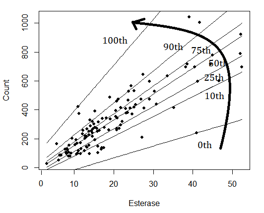
Figure 1: Quantile Regression.

The estimates from a quantile regression produce a separating line that divides the data based on the specified $\tau$. The 0th percentile is a line that is located just below all the data points. Similarly, the 100th percentile is a line that is located just above all the points. The 50th percentile falls in between and conveniently divides the data in half. Other lines shown are for the 10th, 25th, 75th and 90th percentile. Note that as $\tau$ increases from 0 to 1, the slope of the line gets steeper and steeper as it “captures” more and more of the points below it. Essentially, the line sweeps through the points in the radial direction indicated by the arrow.

One natural approach to monitor the quality of a quantile regression method is to simply count the number of data points below a given regression line (or hyperplane in multiple dimensions). The median line (50th percentile) should result in half the points below it. The 75th percentile should results in 75% of the data below that line, and so on. One rule that should be enforced is that a higher percentile will have more points below it than a lower percentile. That is, we should not have more points below the 75th percentile than we do at the 80th percentile. This would violate the basic definition of percentiles, which is not desirable. Unfortunately, this type of non-monotonic behavior can occur with quantile regression, called the crossing problem, as we will discuss shortly.

III-B The Check Function

The question of how to produce the desired regression lines (or hyperplanes) was first addressed by Koenker and Bassett in their seminal paper [1] using a formulation commonly referred to as the check function which can be written concisely as follows:

$$\rho_{\tau}(r_{i},\tau)=\begin{cases}-(1-\tau)r_{i}&\quad\text{if }r_{i}<0\\ \tau r_{i}&\quad\text{if }r_{i}\geq 0\end{cases}$$ (3)

where the scale $\tau\in(0,1)$ is the quantile of interest and $r_{i}$ is the $i$th residual. Different regression quantiles represented by lines or hyperplanes are obtained by selecting $\tau$ and minimizing the conditional quantile function

$$Q_{C}(Y|x,\tau)=\sum_{i=1}^{n}\rho_{\tau}(r_{i},\tau).$$ (4)

This approach will be referred to as RQ in this paper. A plot of $\rho_{\tau}(r_{i},\tau)$ for different values of $\tau$ is provided in Fig. 2. Suppose we are interested in the median, which is also the 50th percentile and the 2nd quartile.

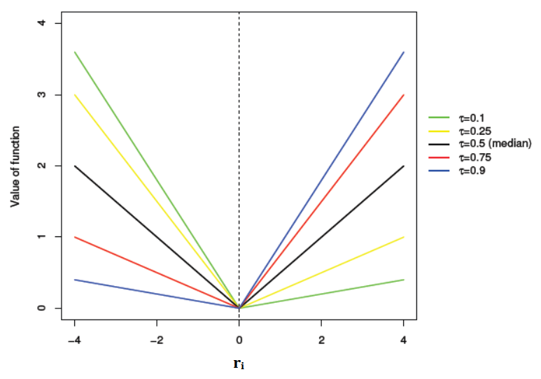
Figure 2: Check function.

We would set $\tau=0.5$ and use the following check function,

$$\rho_{\tau}(r_{i},0.5)=\begin{cases}-(0.5)r_{i}&\quad\text{if }r_{i}<0\\ 0.5r_{i}&\quad\text{if }r_{i}\geq 0.\end{cases}$$ (5)

This is equivalent to the least absolute deviation (LAD) function or the L1 loss function. We see from the figure (black line, $\tau=0.5$) that it is symmetric about $r_{i}=0$ but has a kink at 0. This is the same characteristic that causes problems with the L1 function. Because of this kink, the derivative of this function is discontinuous at 0. There are mathematical and numerical issues around using it. However, for quantile regression, the problem is somewhat exacerbated as there are many percentiles and quantiles to consider, other than just the 50th percentile, and they all have discontinuous 1st derivatives, and undefined 2nd derivatives.

For further illustration, suppose we are interested in the 3rd quartile or 75th percentile. Then we should set $\tau=0.75$ as follows:

$$\rho_{\tau}(r_{i},0.75)=\begin{cases}-(0.25)r_{i}&\quad\text{if }r_{i}<0\\ 0.75r_{i}&\quad\text{if }r_{i}\geq 0.\end{cases}$$ (6)

This produces the asymmetric plot that looks like a check mark as shown in red for $\tau=0.75$ in Fig. 2. This is where the function gets its name; the red lines resemble a check mark. For other percentiles or quantiles, it simply requires setting $\tau$ to a different value, as shown in the figure. Unfortunately, the functions are not smooth and their derivatives are not continuous. Every one of them has a kink and a resulting discontinuity in the first derivative. When minimizing a loss function constructed from this check function, one must resort to linear programming techniques such as the simplex-type or interior point methods to obtain a solution and unfortuantely this presents a problem as discussed in the next section.

III-C The Crossing Problem

There are countless papers written about the crossing problem and how to circumvent it, including [3][4][5][6][7][8][9][10][11][12], to name a few. The basic issue is shown in Fig. 3 and can be contrasted with Fig. 1. We see that the two lines shown intersect, i.e. cross, and this has implications in the resulting monotonicity of the percentiles. Not all cases where lines cross actually present a problem, but the implication is that when two lines cross in the convex hull of the data, something went wrong. A higher number of points may be captured by a lower quantile line as compared to the higher quantile line. Therefore, the crossing problem is manifested as a non-monotonicity problem as percentiles increase. But why would this occur?

We suspect that it is due, in part, to the original formulation of the check function and the techniques used to solve it. The constraints due to linear programming (a finite set of possible solutions) and limited options on small data sets as you increase the percentiles gives rise to a significant part of the crossing problem and, in particular, the systematic component of the error. Regions in the neighborhood of $\tau=0$ and $\tau=1.0$ are particularly prone to it, although the overall solution may exhibit the non-monotonic behavior in any region in between. There is also the possibility of infinite solutions.

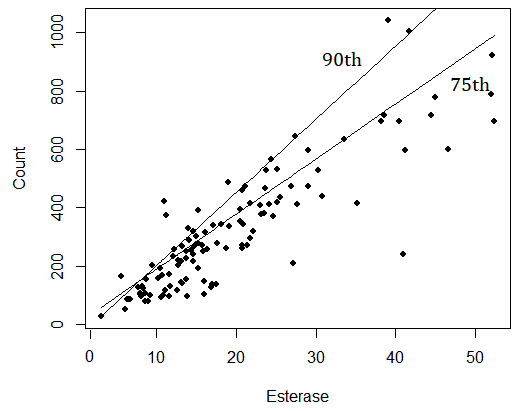
Figure 3: Crossing problem.

Our goal is to find a simple and general solution to avoid crossing. We emphasize here that the lines and hyperplanes from quantile regression will always intersect in some way if they are not parallel. Hence, two lines may cross but the estimated model can be still be viewed as acceptable if the crossing occurs outside the convex hull [2]. Lines crossing within the convex hull often leads to non-monotonicity, but not always, whereas if non-monotonicity is detected, there is implicitly a crossing problem. Therefore, we need a way to monitor any non-monotonic behavior in quantile regression to evaluate the performance of different approaches.

IV Systematic Regression Quantiles (SRQ)

IV-A Continuous L1 Function

The starting point for a new approach to quantile regression is to find a way to construct a continuous function with continuous derivatives to replace the check function which has discontinuous derivatives. Consider first how one might replace the L1 function with a continuous counterpart. This is shown in Fig. 4 using a variable, say $x$. The absolute value function, $|x|$, has a “V” shape. When we take its derivative, we obtain sgn($x$) which is discontinuous at $x=0$. We can construct a continuous version of it using tanh($10x$). To the naked eye, they look the same but one is discontinuous and the other is continuous. Then, by integrating the function, we obtain $\frac{1}{10}$log(cosh($10x$)) which does not have a kink although it may appear to have one in the figure. For robust regression, this function can be used as an alternative to LAD.

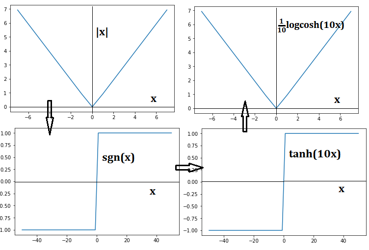
Figure 4: Developing a continuous L1 function.

IV-B Continuous Check Function

Now that a procedure is established to create continuous functions that look like their piecewise-linear counterparts, we merely repeat the process for the check function. First we take the check function of (3) and plot it as shown in Fig. 5 in the top left panel for 11 quantiles (0, 1, and all the deciles in between). Next we take its derivative to obtain

$$\rho_{\tau}^{\prime}(x,\tau)=\begin{cases}-(1-\tau)&\quad\text{if }x<0\\ \tau&\quad\text{if }x\geq 0.\end{cases}$$ (7)

This is shown in the bottom left panel. These are all discontinuous step functions. We need to create a continuous version of the derivative of the check function by first scaling the term tanh($10x$) by $1/2$ to match its range, that is,

$$f(x)=\frac{1}{2}\text{tanh}(10x).$$ (8)

Then we can translate it up or down using $\tau$ by adding $(\tau-\frac{1}{2})$,

$$f(x,\tau)=\frac{1}{2}\text{tanh}(10x)+(\tau-\frac{1}{2}).$$ (9)

This is plotted in the bottom right panel. Finally, we integrate this function to obtain the continuous check function of the form given earlier in (1):

$$F(x,\tau)=\frac{1}{20}\text{log}(\text{cosh}(10x))+(\tau-\frac{1}{2})x.$$ (10)

This is plotted in Fig. 5 in the top right panel. The use of (10) for quantile regression will be called systematic regression quantiles (SRQ) in this paper.

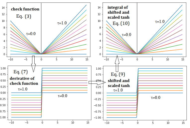
Figure 5: Developing a continuous check function.

IV-C Simple Linear Regression Example

We will now compare RQ and SRQ on a simple linear example from the anscombe data set in R. Using the $y1$ and $x2$ values, a scatter plot for the 11 points in the data set is shown at the top of Fig. 6 with the median line ($\tau=0.5$) shown for both RQ and SRQ. They are about the same, although on closer inspection, there is a slight difference. The programs used are rq from the quantreg library in R and srq, our own R program based on (10).

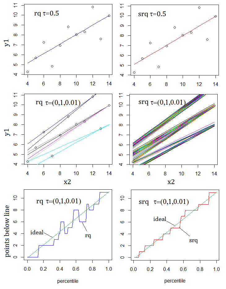
Figure 6: Comparison of RQ and SRQ on anscombe data.

In the middle panels, all 100 regression lines, one-per-percentile, are plotted. This is a surprising statement since the middle-left panel appears to only have 10 or 11 lines plotted, whereas the middle-right plot seems to have many lines plotted (and in fact 100 lines). It is clear that RQ does not produce 100 distinguishable lines for the 100 percentiles in this case because it is being hindered by the limited number of options from linear programming.

On the other hand, SRQ has the luxury of finding any solution in a continuous space and therefore produces 100 different lines for the 100 percentiles. This is the key benefit of SRQ over RQ. In a continuous space, any point is a potential solution, whereas in the space defined by a set of linear functions with linear constraints, solutions are permitted only at the vertices of the constraints, or perhaps an infinite number of solutions are possible which is also unsatisfactory. This is the major reason for the non-monotonicity problem encountered in standard quantile regression.

One issue with the linear plots of the middle panels is that it is difficult to observe the crossing problem directly because the lines are too close to each other. We propose a new way to assess the overall performance of a quantile estimator by simply counting the number of points below a given line. For example, the 0th percentile line should have 0 points below it, while the 100th percentile line should have all 11 points below it in this example. Then, as the percentile increases from 0 to 100, the number of points should increase monotonically from 0 to 11. If this does not happen, then the desired monotonicity property of percentiles is violated. Such a plot of “points below line” against $\tau$ is reminiscent of the Q-Q plot and can be interpreted in the same way. Hence, the ideal line is a diagonal line from corner to corner as in a typical Q-Q plot. We will use this type of Q-Q plot extensively to compare different methods in the remainder of this paper.

The third pair of plots at the bottom of Fig. 6 shows the Q-Q type results for RQ and SRQ using the quantiles $\tau=0.01,0.02,...,0.99$ which is represented as $\tau=(0,1,0.01)$ in the figure. We can observe the significant amount of non-monotonicity of RQ whereas SRQ closely tracks the ideal solution using an “uneven staircase”. The ideal line is the diagonal that connects (0,0) to (1.0,11), the two known solution points, which are interpolated as shown in green. SRQ is monotonic over the entire interval. RQ features 3 non-monotonic cycles over the same interval.

V Comparison with RRQ

A number of techniques for solving the crossing problem have been attempted in the past with varying degrees of success. Two different approaches have been taken: (1) Reduce the crossing problem by applying some constraints or restrictions on the problem, and (2) Apply some smoothing or fitting method for a number of quantiles over a given interval. See [5] for a summary of various methods.

We will first compare SRQ with a well-known approach referred to as the Restricted Regression Quantiles (RRQ) method [3][7]. RRQ as described in [3] is a three-step method as follows. Consider the linear heteroscedastic model given by:

$$y=x^{\prime}\beta+(x^{\prime}\gamma)e$$ (11)

where $e$ is any error distribution. For RRQ, first solve the quantile problem for the median case to obtain $\hat{\beta}$ and $r_{i}$. Next, regress $|r_{i}|$ on $x_{i}$ to obtain the median regression coefficients $\hat{\gamma}$ and the corresponding fitted values which are $s_{i}=x_{i}^{\prime}\hat{\gamma}$. Then, finally, we find $c_{\tau}$ by minimizing $\sum\rho_{C}(r_{i}-cs_{i})$ over $c$ to produce the $\tau$th hyperplane as $y=x^{\prime}(\hat{\beta}+c_{\tau}\hat{\gamma})$, which is the so-called RRQ estimator. This approach is implemented in a program called rrq in the Qtools library in R.

If we compare RRQ to SRQ on the esterase assay data set in R containing 113 observations and only 1 explanatory variable, we observe in the Q-Q plots of Fig. 7 where RRQ is locally non-monotonic in two instances (called spikes in this paper) whereas SRQ is monotonic for all quantiles shown. Hence, for this data set SRQ is the preferred option for quantile regression.

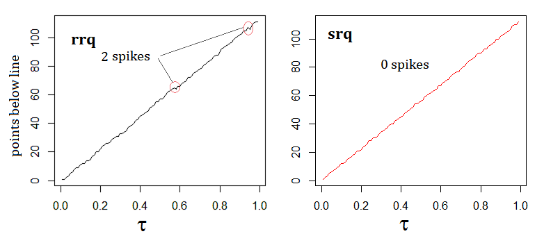
Figure 7: Comparison of RRQ and SRQ on esterase assay data.

VI Random Error Suppression

While the SRQ approach circumvents the need for linear programming, thus avoiding the systematic part of the crossing problem, unfortunately it does not remove the crossing problem entirely. This is partially due to the fact that random errors may arise from the data itself. However, these random errors tend to be localized by SRQ and can be removed in a variety of ways. Techniques for fitting and local smoothing are now tractable since most of the errors are single-event errors (called spikes and pulses) whereas these techniques are not as effective on the non-monotonic behavior of RQ or RRQ, which can be global in nature, especially in small data sets.

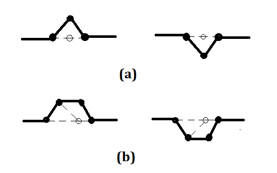
Figure 8: Non-monotonic event suppression: (a) spikes (b) pulses

There are two types of local non-monotonic events that can be handled easily as shown in Fig. 8. The single-event positive or negative spikes (solid lines) of Fig. 8(a) can be suppressed (dotted lines) by examining 2 neighboring quantiles. The single-event positive or negative pulses (solid lines) of Fig. 8(b) can be converted to spikes, as shown (dotted lines), or removed by considering multiple neighboring quantiles. The details are not important here but the process of suppressing these events is tractable. If the pulse width exceeds 2 quantiles, more advanced methods are required. The kernel-based and other fitting approaches [8] would be effective in those cases.

To demonstrate this approach, consider the swiss data set with $n=47$ observations and $p=5$ explanatory variables. We show the Q-Q plots from quantile regression using RQ, RRQ and SRQ in the top two panels and bottom-left panel, respectively, in Fig. 9. Notice the severity of the non-monotonic behavior for RQ. It is reduced using RRQ, and further reduced using SRQ, but not eliminated. Both RQ and RRQ exhibit “global” non-monotonicity, i.e. something that cannot be fixed by examining a local region alone. There are 6 spikes in SRQ that can be removed by simply examining the nearest quantile neighbors and suppressing them to avoid crossing planes. This is shown in the bottom-right panel of Fig. 9 which is referred to as SRQ-S since spike suppression has been applied here.

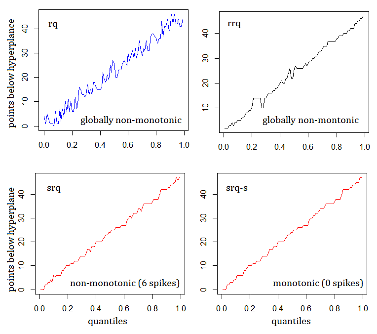
Figure 9: Comparison of RQ, RRQ, SRQ and SRQ-S on swiss data.

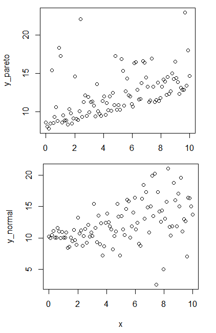
Figure 10: Examples of pareto and normally distributed noise for data with 100 points.

TABLE I: Comparison of rq, rrq and srq on simple linear regression quantiles for different data sizes (pareto).

Data	Technique Used
Points	rq	rrq	srq
20	2/1	6/1	0/0
40	8/4	7/0	0/0
60	10/1	1/0	0/0
100	6/0	1/0	0/0
400	0/0	0/0	0/0

TABLE II: Comparison of rq, rrq and srq on simple linear regression quantiles for different data sizes (normal).

Data	Technique Used
Points	rq	rrq	srq
20	2/3	6/1	1/0
40	3/4	10/1	1/0
60	13/0	4/0	0/0
100	6/0	2/0	0/0
400	0/0	0/0	0/0

In the next series of comparisons, we use will use two cases that are particularly problematic for standard least squares linear regression. Synthetic data are created in two ways with heteroscedastic normal noise added and asymmetric pareto noise added, respectively, for different numbers of observations (i.e. 20, 40, 60, 100 and 400). Examples from each set using 100 data points are shown in Fig. 10.

The comparison of RQ, RRQ and SRQ involves counting the number of single-event spikes and pulses (of width two or more) over the range of quantiles, $\tau=(0,1,0.01)$. In Tables I and II comparing rq, rrq and srq, the first number for each is the number of spikes while the second is the number of pulses. We can observe that rq and rrq have a larger number of such events for small data sets but it is reduced as the size increases. For srq, the performance is near-perfect in all cases shown, and can be made perfect using suppression since they are all single-event spikes, and very few in number.

VII Smoother Check Functions

While the results thus far are interesting, it can be improved further through the use of a smoother check function, as described in this section. It is particularly effective in removing non-monotonicity that has to do with resolution and sensitivity [5]. In particular, if quantiles are spaced 0.001 units apart, then a total of 1000 quantiles are required in the range $(0,1)$. The estimation process may not have the resolution to produce monotonic behavior using SRQ.

Consider the swiss data set once again. We show the results of 1000 quantile regressions in Fig. 11. The effects of the fine resolution has exacerbated the effects of non-monotonicity compared to Fig. 9 which was based on 100 quantile regressions using spacings of 0.01. RQ and RRQ now exhibit much more non-monotonicity. The root cause of this excessive non-monotonic behavior is the quantile spacing. The kink is the source of much of the crossing problem in classical quantile regression. Although SRQ rounded the kink out to make the function continuous, that is still not sufficient for high resolution quantile regression. Therefore, an adjustment is required to further smoothen the kinks for the cases where very fine-grain results are desired.

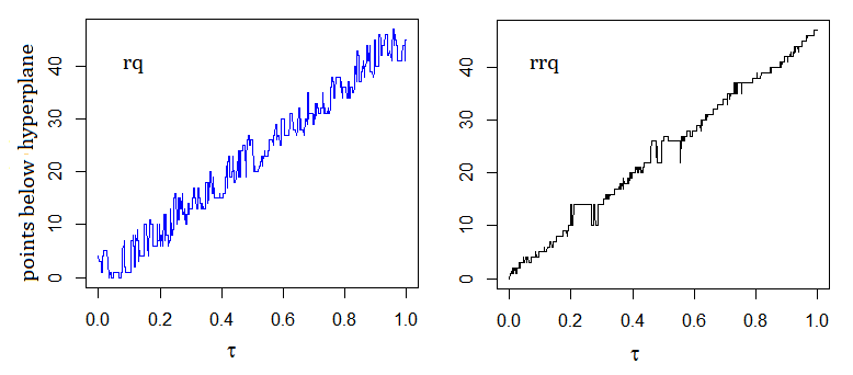
Figure 11: Effect of closely spaced quantiles using swiss data.

VII-A Flexible Check Function

In this section, we introduce a new approach that smooths out the loss function. We described the use of the logcosh function to replicate the original check function to round out the kink. We use the same type of equation to allow more smoothing. Its most general form is the key contribution of our paper as shown in Fig. 12 and given by:

$$F(x,\tau)=\frac{1}{2c}\text{log}(\text{cosh}(c(x-h)))+(\tau-s)x+v$$ (12)

where $c$ is the desired curvature of the function (i.e. the severity of the kink), $v$ controls vertical shift, $h$ controls the horizontal shift and $\tau-s$ is used to produce the desired slopes on the two sides of the check function itself.

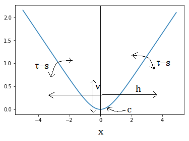
Figure 12: Parameters of flexible check function.

In the case of the continuous check function, we set $c=10,h=0,s=0.5$ and $v=0$. However, for a smoother check function, we can use $c=0.7,h=0,s=0.5$ and $v=0.4$ which produces the following

$$\rho_{SM}(r_{i},\tau)=\frac{5}{7}\text{log}(\frac{7}{10}\text{cosh}(r_{i}))+(\tau-\frac{1}{2})r_{i}+\frac{2}{5}$$ (13)

where $r_{i}$ is the $i$th residual as before. The method using the above equation is referred to here as SMRQ for ‘smoother quantiles’. Fig. 13 shows five different cases of (12) by varying parameters $c$ and $v$ (while holding $s=0.5$ and $h=0$ fixed), including SRQ of (1) and SMRQ of (13) for $\tau=0.5$ and $\tau=0.7$. One can observe the different levels of smoothness offered by the flexible check function, which can be varied easily as the need arises.

Figure 13: Loss functions for SRQ and SMRQ for $\tau=0.5$ and $\tau=0.7$ cases.

Recently, a technique was published that utilizes convolutional smoothing applied to the loss function (He et. al., 2020) and is implemented in the conquer library in R [12]. Convolutional smoothing provides a different approach to reducing the crossing problem. A comparison of conquer against smrq is shown in Fig. 14. It is the swiss example with $n=47,p=5$ and quantile spacing of 0.01 and 0.001, respectively. We can observe 1 non-monotonic event for the 100 quantile case and 3 non-monotonic events in the 1000 quantile case for conquer, whereas there are none in either case for smrq. We find that smrq is generally monotonic in small sample data for all quartiles, deciles and percentiles.

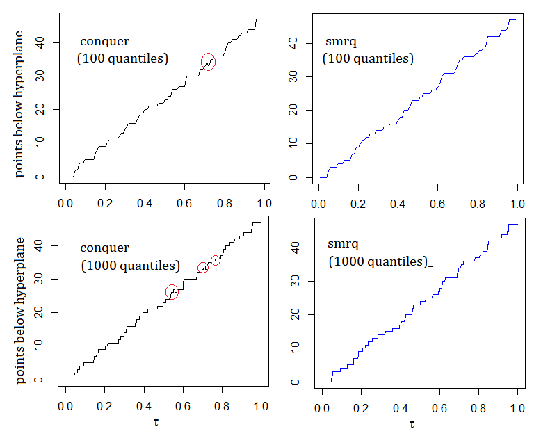
Figure 14: Comparison of conquer and smrq on swiss data. Red indicates a non-monotonic spike event. No pulse events occur.

We now illustrate large-sample data and high-resolution cases using the diabetes data with 442 observations and 10 variables, and the Boston housing data [5] set with 506 observations and 15 variables. The number of non-monotonic events (both spikes and pulses) are fewer for conquer compared to smrq. However, if noise supression is applied to smrq, as described earlier, then smrq-s is superior to conquer.

TABLE III: Comparison of conquer, smrq and smrq-s on diabetes data for different quantile sizes.

No. of	Technique Used
Quantiles	conquer	smrq	smrq-s
100	0/0	0/0	0/0
200	0/0	8/0	1/0
300	20/1	37/5	3/0
400	35/2	90/12	12/1
500	48/3	108/19	19/4

TABLE IV: Comparison of conquer, smrq and smrq-s on Boston Housing data for different quantile sizes.

No. of	Technique Used
Quantiles	conquer	smrq	smrq-s
100	0/0	0/0	0/0
200	0/0	8/2	1/0
300	2/0	17/3	3/1
400	6/0	38/10	4/1
500	4/0	65/14	15/2

VIII Conclusions

In this paper, we have addressed the non-monotonicity problem due to line and hyperplane crossing in quantile regression. We introduced a unique flexible check function and used standard nonlinear optimization to obtain quantile estimates rather than linear programming. The new method is a simple way of undoing the crossing problem. We compared the baseline method called SRQ with RQ and RRQ to demonstrate that it is substantially better. Next, we developed a smoothing and suppression approach, called SMRQ-S, to further reduce the crossing problem. It was shown to outperform the convolutional smoothing approach used in conquer. Finally, we provided cogent explanations of the root causes of the crossing problem. In summary, smoothing out the kinks and suppressing spikes reduces the crossing problem significantly in quantile regression. A portion of our R code is provided in the Appendix using the swiss data set for evaluation purposes.

IX Appendix: R code for Swiss data

####################################################### This contains the Swiss data sets for quantile     ## regression comparing rq, rrq, conquer and smrq     #######################################################library(quantreg)library("limma")library("Qtools")library("conquer")swiss <- datasets::swissx <- model.matrix(Fertility~., swiss)[,-1]y <- swiss$FertilityX <- cbind(x,rep(1,nrow(x)))minimize.logcosh <- function(par, X, y, tau) {  diff <- y-(X %*% par)  check <- (tau-0.5)*diff+(0.5/0.7)*logcosh(0.7*diff)+0.4  return(sum(check))}smrq <- function(X, y, tau){  p = ncol(X)  op.result <- optim(rep(0, p),            fn = minimize.logcosh,            method = ’BFGS’,            X = X,            y = y,            tau = tau)    beta <- op.result$par    return (beta)}n <- 99             #choose 99 or 999p = ncol(X)vals0 <- rep(0,n)vals1 <- rep(0,n)vals2 <- rep(0,n)vals3 <- rep(0,n)alphas <- rep(0,n)for (i in 1:n) {    alpha = i/(n+1)    alphas[i] = alpha    betas <- smrq(X,y,tau=alpha)    vals0[i] <- sum(y<(X %*% betas))    model_qr<-rq(Fertility~.,data = swiss,tau=alpha)    vals1[i] <- sum(swiss$Fertility <              model_qr$fitted.values)    fitr <- rrq(Fertility ~ ., data = swiss, tau = alpha)    vals2[i] <- sum(y < predict(fitr))    alpha1 <- 1.0 - alpha    fitc <- conquer(x,y,tau = alpha1)    vals3[i] <- sum(0 <fitc$residual)}par(col=1,mfrow = c(2, 2))plot(alphas, vals1, type = "l", col = 2,main=’rq’)plot(alphas, vals2, type = "l", col = 1,main=’rrq’)plot(alphas, vals3, type = "l", col = 1,main=’conquer’)plot(alphas, vals0, type = "l", col = 4,main=’smrq’)

References

- [1] Koenker, R., and Bassett, “Regression Quantiles,” Econometrica 46, 33-50 (1978).
- [2] Koenker, R., Quantile Regression, Cambridge University Press, 2005.
- [3] He, X., “Quantile Curves without Crossing”, The American Statistician 51, 186-192 (1997).
- [4] Bondell, H.D., B.J. Reich and X. Wang, 2010, “Noncrossing quantile regression curve estimation”, Biometrika, 97: 825-838.
- [5] Amerise, I., “Quantile Regression Estimation Using Non-Crossing Constraints”, Journal of Mathematics and Statistics, Volume 14: 107-118, 2018.
- [6] Wu, Y. and Liu, Y. “Stepwise multiple quantile regression estimation using non-crossing constraints” Statistics Interface, 2: 299-310, 2009.
- [7] Zhao, Q., “Restricted regression quantiles”. Journal of Multivariate Analysis, 72: 78-99, 2000.
- [8] Yu, K. and Jones, M. C. “Local linear quantile regression” Journal of the American Statistical Association, 93: 228-237, 1998.
- [9] Neocleous, T. and Portnoy, S. “On Monotonicity of Regression Quantile Functions”, Statistics and Probability Letters, 78: 1226-1229, 2007.
- [10] Bassett, G. and R. Koenker, “An empirical quantile function for linear models with iid errors”, Journal of the American Statistical Association, 77: 407-415, 1982.
- [11] Chernozhukov, V. and Fernandez-Val, I. and Galichon, A., “ Quantile and probability curves without crossing”, Econometrica 78, 1093-1125, 2010.
- [12] He, X., Pan, X., Tan, K. M., and Zhou, W., “Smoothed Quantile Regression with Large-Scale Inference”, arXiv:202.05187v1, 2020.