Abstract

Benefiting from expanding cloud infrastructure, today’s deep neural networks (DNNs) have increasingly high performance when trained in the cloud. Researchers spend months of effort competing for an extra few percentage points of model accuracy. However, when these models are actually deployed on edge devices in practice, very often, the performance can abruptly drop over 10% without obvious reasons. The key challenge is that there is not much visibility into ML inference execution on edge devices, and very little awareness of potential issues during the edge deployment process. We present ML-EXray, an end-to-end framework which provides visibility into layer-level details of the ML execution, and helps developers analyze and debug cloud-to-edge deployment issues. More often than not, the reason for sub-optimal edge performance does not only lie in the model itself, but every operation throughout the data flow and the deployment process. Evaluations show that ML-EXray can effectively catch deployment issues, such as pre-processing bugs, quantization issues, suboptimal kernels, etc. Using ML-EXray, users need to write less than 15 lines of code to fully examine the edge deployment pipeline. Eradicating these issues, ML-EXray can correct model performance by up to 30%, pinpoint error-prone layers, and guide users to optimize kernel execution latency by two orders of magnitude. Code and APIs will be released as an open-source multi-lingual instrumentation library and a Python deployment validation library.

1 Introduction

Driven by continuous advances in machine learning (ML) techniques, ML-based systems have been increasingly deployed to accomplish a variety of tasks. With the rise of the Internet of Things (IoT), the endless sensory data stream from edge devices to the cloud helps train ML models to achieve higher and higher performance. In addition to sitting on the cloud serving inference requests, recent years have seen these high-performance models widely deployed back on actual devices at the edge, to enable low-latency, low-power, privacy-sensitive applications (e.g., autonomous vehicles, personal assistants, video analytics etc.).

However, deploying these ML applications on the edge poses new challenges, specifically due to compute hardware heterogeneity, environmental variations, and sensor variations Cidon et al. (2021). These issues are not well addressed, partly because there is a disconnect between the people who develop the models in the cloud and those who deploy the model on edge devices. This disconnect is deeply rooted because the design goals are not exactly the same: the objective of training is heavily focused on accuracy whereas the deployment prioritizes efficiency and end-to-end system performance. There are a lot of design choices being made when people are training and improving the model in the cloud that are not well documented and are lost in the handoff to the app development and deployment team. Even if there was a good handoff, the heterogeneity at the edge can be in conflict with those design choices.

This disconnect can be critical to efficient and successful deployment. For example, a popular internet search company has been experiencing significantly degraded performance (see §4.3) when they deploy their vision-based ML applications using popular models (e.g., MobileNet Howard et al. (2017)). A large social media company finds that some well-trained neural networks, when quantized and deployed on their app, are not working for particular chips (see §4.4). It is very hard to pinpoint where the problem lies. More often than not, not only the operations (Ops) in the model could be error-prone when executed on heterogeneous devices, but also bugs throughout the whole pipeline (e.g., preprocessing, postprocessing, model optimization, quantization).

What exacerbates the situation is that it is very challenging to debug the problems caused by this disconnect. There is neither any visibility into, nor any reference of, what is happening when models are executed at the edge. Without proper deployment benchmarks, many of these issues will just slip by silently. Take image classification models (e.g., Keras classification models ker ) as an example. A MobileNet model takes an RGB image of $[-1.0,1.0]$ as input, whereas a VGG Simonyan & Zisserman (2014) model takes a BGR image, and a DenseNet Huang et al. (2017) model takes $[0.0,1.0]$ inputs. These input mismatches will not trigger any run-time errors, but can affect model performance silently( §4.3). Even for those issues caught belatedly, due to the lack of visibility, and the asymmetric information/assumptions from the disconnect, it takes weeks and even months to debug. The engineers have to manually log the output from any ops they suspect from the complicated neural network graph. Then they verify these logs against a correct pipeline, often developed by themselves as well. The process is extremely laborious and cumbersome.

To provide visibility and help facilitate debugging edge ML systems, we present ML-EXray, a cloud-to-edge deployment validation framework. ML-EXray enables app developers to discover and locate possible issues faster and provide root-cause analysis when possible. Specifically, ML-EXray 1) scans model execution in edge ML apps by logging intermediate outputs, 2) provides a faithful replay of the same data using a reference pipeline, 3) compares performance differences and per-layer output discrepancies, and 4) enables users to define logging around custom functions, write custom reference pipelines, and write custom assertions to verify suspicious model behaviors.

We implement ML-EXray as a suite of instrumentation APIs and a Python library. Evaluations are conducted across image, audio, and text-based ML applications using widely deployed models and public benchmark datasets. Instrumenting and deploying these applications on mobile devices, we found that ML-EXray can effectively catch a variety of deployment issues that the industry has been suffering, including preprocessing bugs, model optimization and quantization issues, and abnormal execution latency. Some of these issues, such as malfunctioning quantization ops, were not previously discovered, and have been reported and are now on the developer teams’ road map to be fixed. To catch these issues using ML-EXray, users would only need to write less than 5 lines of code (LoC) of app instrumentation, and less than 10 LoC of assertion functions. The overhead of ML-EXray during runtime is only up to 3ms per frame (2.3% if running the model on CPU, 15% if on GPU), consuming up to 4 MB memory (compared to a typical ML model footprint of 15 to 100 MB).

A major usage of ML-EXray is to trigger per-layer examination and check user-defined assertions to quickly and effectively catch the issues mentioned above. For example, comparing against the reference pipeline step by step, a difference after normalization op can verify if the scaling is correct, a difference after a quantized layer can alert a quantization issue, a comparison after permuting the channels of the preprocessing output can verify if RGB channel was arranged as BGR. All of the per-layer logging and assertions can be run offline efficiently. Resolving these issues, our evaluations show that ML-EXray can help users 1) significantly correct app performance (e.g., improving model accuracy by up to 30%), 2) pinpoint buggy ML operations (e.g., quantized depthwise convolution layer, quantized average pooling layer), and 3) shorten execution latency.

In summary, we make the following contributions:

• We introduce edge ML instrumentation APIs, providing visibility into layer-level details on edge devices.

• We provide an end-to-end edge deployment validation as an abstraction, giving users an interface to design custom assertions for deployment verification.

• We show that ML-EXray can catch various deployment issues in large-scale industrial production pipelines across tasks of different data modalities.

• We demonstrate the impact of these previously invisible issues, and how ML-EXray makes it easy to catch these issues, raising the awareness of deployment debugging.

Code and APIs will be open-sourced to the community.

2 ML Deployment on the Edge

In this section, we describe the Edge ML deployment process and challenges experienced by our industrial partners during their large-scale deployment. We use these critical deployment issues as case studies throughout the paper. Deploying pre-trained ML models usually involves three major steps: 1) develop an ML inference pipeline on the target edge platform, 2) convert ML checkpoints to executable versions, and, when necessary, quantize models to fit hardware specifications, and 3) validate model performance and debug potential deployment issues.

ML Inference Pipeline on the Edge. At the core of an ML application is an inference pipeline, which applies edge device sensory data to a pre-trained ML model to perform an automated task. A typical pipeline includes sensor capture (e.g., image, audio, text, point cloud, etc.), data pre-processing (e.g., resizing, normalization, voxelization), invoking the ML model, and finally post-processing results.

Take an android image classification app as an example. The app captures images from the camera, extracts RGB channels from the image byte array, resizes it to the model’s input size, converts the input to the numerical format expected by the model, forwards the data to the input tensor, invokes the model, gets the output class of the highest score, and finally reports the corresponding image category.

It is extremely challenging for app developers to write such a pipeline without any bugs, especially for the data preprocessing stage. Essentially, they have to create new code that emulates what happens in the training pipeline exactly, with no easy way to check that they’re doing it correctly.

From conversations with engineers in industry responsible for shipping on-device ML products, we’ve identified several categories of errors that are common in real products and are currently hard to detect. These can most easily be illustrated using examples from the Android image classification example described above.

Channel extraction. Images are natively stored according to a channel arrangement (e.g., YUV, BGR, etc.) that differs from that expected by the DNN. Bugs in the conversion process can affect the results. Even if the channel is arranged correctly, the library being used to extract the RGB values can be important, since there can be differences in color space and gamma conversions Wallace (1992).

Resizing. Camera captured images are almost certainly not the right size for the network’s input, and will probably need to be scaled down. In the early days, instead of an area-averaging downsampler, a lot of researchers just used a default of bilinear resampling, which can introduce a lot of aliasing Savsunenko (2018). This mismatch proved to lose a decent amount of top-1 accuracy, as we show in §4.3.

Numerical conversion. Color values are usually expressed as unsigned integers, but DNNs usually want floating point values in the training environment. This conversion usually happens deep in the internals of the training framework, of which the model author is unlikely to be aware, and so isn’t able to pass along the information to the mobile app developer even if they wanted to. It is tricky to detect such a mismatch. For example, if the network expects $[-1.0,1.0]$ and the conversion produces $[0.0,1.0]$, it will just appear as a washed-out image and so recognition will somewhat appear to work, just with a big loss of accuracy (see §4.3).

Orientation. The input image, either landscape or portrait, always has the correct orientation during training. However, when edge devices capture image data, the orientation can change. Some networks may be trained with data augmentation, such as random rotations or horizontal/vertical flips. Our evaluation (§4.3) shows that many popular classification models suffer from a 90 degree rotation of the input.

The same challenges also exist in apps with other input types such as audio, accelerometers, point clouds, RF signals. These sensor modalities typically require a lot more explicit feature generation in the preprocessing stage, such as FFTs yam , voxelization Zhou & Tuzel (2018), etc. Usually, this feature generation work, implemented outside of the ML model graph, is not available to app developers.

Model Optimization and Quantization. The most important module in the edge ML inference pipeline is the neural network itself. When deploying these models on edge devices, it is crucial to optimize Han et al. (2016); tfm these models for inference purposes as they come typically from a training pipeline. In contrast to a training environment, edge devices often have limited compute resources and memory. Fortunately, app developers have a plethora of choices to optimize the model. For example, to invoke these pre-trained DNNs efficiently on edge devices, training-related features and operations are removed and the network is optimized with techniques such as constant folding (including batch normalization folding) and fusion (including fusion of activation function, such as ReLU). Additionally, edge ML systems usually use light-weight interpreters to replace the full TensorFlow run-time David et al. (2021).

One of the most common optimizations is model quantization Jacob et al. (2017); Krishnamoorthi (2018): converting model weights and biases from 32-bit floats to lower precision values (e.g., 16-bit floats for GPUs, 8-bit integers for Edge TPUs). Quantization offers faster arithmetic, reduces memory, disk, network, and battery consumption, and enables running models on hardware accelerators, some of which do not support floating-point operations. Quantization has been successfully applied to many model operations Shangguan et al. (2019) and architectures Li & Alvarez (2021). In the most simple format (asymmetric, per-tensor quantization), the equation to quantize 32-bit floats to unsigned integers and reconstruct back is:

$$quantized=uint8\left(\frac{original-min}{max-min}\times 255\right)$$ (1)

$$reconstructed=\frac{quantized}{255.0}\times(max-min)+min$$ (2)

where $max$ and $min$ are the profiled range of the tensor value. In reality, the details are much more complicated than the equations and we select a few outstanding reasons:

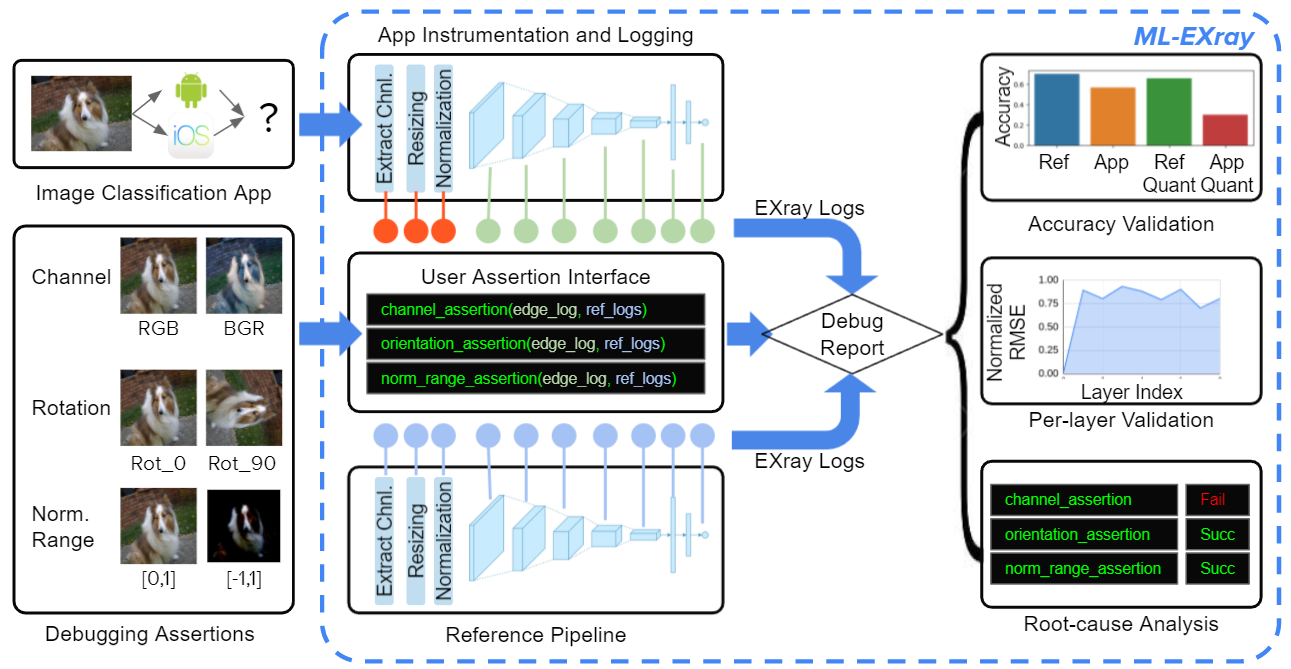
Figure 1: An Overview of the ML-EXray System. (1) App developers use ML-EXray APIs (§3.2) to instrument mobile apps (e.g., an image classification app) to produce EXray logs (default logs (green) and custom logs (red)). (2) ML-EXray plays back the same data using a reference pipeline (§3.3) and produces the same user-defined logs. (3) Users define debugging assertions (§3.4) like input channel arrangement, orientation, and normalization range. (4) ML-EXray compares edge logs with reference logs (§3.4), and reports potential issues like accuracy degradation, per-layer output drift, as well as root-cause assertion results.

Scale calibration. The $min$ and $max$ from Eqn. 1, 2 for each tensor is unknown to app developers. Quantization tools typically require example input data for calibration. In this case, an outlier in the representative dataset could inflate the scale such that quantized integers do not have enough resolution to tell the difference generated by normal input data. In contrast, a small example dataset could render the scale too small such that values generated by normal input data are clipped by integers 0 and 255.

Symmetric quantization. For a given tensor, asymmetric quantization utilizes the full int8 range while symmetric quantization uses a fraction when data is skewed. However, in practice, symmetric quantization is widely used, allows better optimization on ARM CPUs, and the absence of zero point translates to better performance Nagel et al. (2021).

Per-tensor vs per-channel quantization. The weight distribution in a tensor plays a key role in the accuracy of the model. After batch normalization weight folding, the weight in a convolution or a fully-connected (FC) layer can sometimes be very different from channel to channel. In this case, per-tensor quantization can squash the entire channel to 0 due to the scale difference, whereas per-channel quantization allows each channel to have its own scale and zero point.

Debugging ML Deployment on the Edge. Depending on the severity of these issues described above, model performance can vary from somewhat working (with much lower precision) to not working at all, i.e., outputting constant values (see §4). At the same time, multiple issues can exist together, leaving app developers clueless to debug. Moreover, even though there are run-time ML benchmarking Reddi et al. (2020a; b) and debugging Kang et al. (2018) tools assuming a correct deployment, there are few tools to help figure out if there is any problem lying in the deployment process. App developers would have to manually log and inspect specific tensors, e.g., function outputs, quantized model weights and operation outputs, and check them with the original model given the same input. This process is extremely tedious and laborious, and demands significant deployment experience and domain knowledge.

3 ML-EXray

To provide visibility into and solve edge ML deployment issues, we propose ML-EXray, an edge ML deployment validation and debugging framework.

3.1 System Overview

ML-EXray consists of three components: 1) a cross-platform API for instrumentation and logging (§3.2) for ML running on the edge and cloud, 2) a reference pipeline (§3.3) for data playback and establishing baselines, and 3) a deployment validation framework (§3.4) to identify issues and analyze root-causes. In addition, ML-EXray is fully customizable to user-defined verification.

Figure 1 shows a system overview. We continue to use the image classification app as an example to describe the ML-EXray system. For example, to verify whether the app has any preprocessing issues, an app developer (user) can use ML-EXray APIs to instrument around preprocessing functions (red dots) in the ML inference pipeline. While running the app, ML-EXray will collect both default inference logs (green dots) as well as custom logs (red dots). In order to validate if there are any preprocessing issues, app developers can insert specific assertions that they suspect. For example, users can write simple debugging assertion functions, such as checking whether the channel arrangement is correct, whether the input orientation is correct, or whether the normalization range is correct. Taking these assertion functions, ML-EXray runs an instrumented reference pipeline and compares the logs. In the example shown in Figure 1, ML-EXray first checks the accuracy (accuracy validation). If there is an accuracy drop, ML-EXray then performs per-layer error analysis to locate the discrepancy (per-layer validation). Finally, it runs all built-in and user-defined assertions (root-cause analysis).

Figure 2 shows a generic debugging flowchart. ML-EXray takes as input the model, the benchmark dataset, and produces the edge logs via instrumentation (§3.2). It runs the reference pipeline (§3.3) using the same model on the same dataset in a non-edge environment (e.g., cloud). A degraded accuracy from the edge logs indicates potential deployment issues. ML-EXray then compares the logs from the mobile and cloud to locate the error-prone ops (§3.4).

For novel tasks or domain-specific verification, ML-EXray provides a user interface to insert domain knowledge via a) adding custom logs, b) writing custom assertion functions, c) providing user-defined reference pipelines as baselines. Taking lane detection as an example, users can add lane location to logs, define lane distance as assertions, and provide special post-processing functions to the inference and reference pipelines. Finally, ML-EXray runs user-defined assertions to incorporate expert domain knowledge for root cause analysis. Next, we detail the three core components.

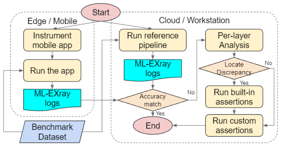
Figure 2: ML-EXray generic deployment validation flowchart. ML-EXray collects logs from instrumented app and reference pipelines and compares them for deployment validation: 1) match the accuracy between two pipelines, 2) If accuracy drops, scrutinize layer-level details and locate the discrepancy. 3) run assertion functions for root-cause analysis.

3.2 API for Instrumentation and Logging

To enable instrumentation on both the edge pipeline as well as the reference pipeline (§3.3), ML-EXray needs to handle the heterogeneity of edge devices. Therefore, ML-EXray provides three sets of APIs: a cross-platform edge API (e.g., c++ for Android, iOS, EdgeTPU), a platform specific API (e.g., Java for Android), and an API for reference pipelines (Python). All the APIs follow the same data model (detailed below), focusing on three types of telemetry data.

As a concrete example, to invoke ML-EXray in a Tensorflow Lite app, a developer may write (in C++):

⬇

MLEXray->on_inf_start();

TfLiteStatus s = m_interpreter->Invoke();

MLEXray->on_inf_stop(&m_interpreter);

Users can also use ML-EXray APIs to log the input and output of any custom functions and peripharal sensors (see appendix §B). For example, to verify if the channels are extracted correctly, users can log the output of the extraction function from the edge pipeline as well as the reference pipeline (denoted as edge_out, ref_out).

We now formulate the data model for logging and give an example of designing assertion functions using the data.

Data model. The API focuses on logging three sets of data:

• Input/Output: including model input/output, per-layer input/output, the input/output of preprocessing and postprocessing functions, as well as the input/output of any user-defined functions in the inference pipeline.

• Performance metrics: including ML inference end-to-end latency, per-layer latency, and memory footprint.

• Peripheral sensors: including the sensors available on the devices, such as orientation, motion, ambient lighting conditions, etc., that may affect input data quality and therefore degrade ML performance.

Each of these can be expressed as a key-value pair.

Assertion function. An assertion function is an arbitrary function that can indicate whether a bug exists or an error happens in the deployed edge pipeline. For various purposes of validation, an assertion function can query different keys in the log of the same pipeline or same keys of two or more different pipelines. For example, the MobileNet model assumes an image input of RGB channel arrangement whereas Inception model assumes BGR. To validate the input channel against a correct reference pipeline for a particular model, an app developer may write (in Python):

⬇

def channel_assertion(edge_out, ref_out) {

if not np.allclose(edge_out, ref_out):

edge_out = cv2.cvtColor(edge_out, cv2.COLOR_BGR2RGB)

if np.allclose(edge_out, ref_out):

raise AssertionError(’BGR->RGB’)}

3.3 Reference ML pipelines and Data Playback

To identify issues of edge ML deployment, we need a correct reference pipeline as the baseline for comparison. However, establishing such baselines can be tricky.

From training an ML model to deployment, the actual model can have multiple versions throughout the entire process. Consider deploying a Tensorflow model to an android app as an example. First, the model presents as several checkpoint files during the training stage. Then, it is converted to one FlatBuffer file to run on the edge devices, while the conversion operation optimizes for inferences. Finally, out of the several quantization schemes Jacob et al. (2017), we consider post-training full-integer quantization, which converts model weights and biases from 32-bit floats to 8-bit and 32-bit integers, suitable for edge deployment.

To establish reference baselines, a first challenge is to have reference pipelines that can faithfully replay data using all these diverse versions of the model described above. For example, a comparison between a checkpoint model and a quantized model can potentially identify issues that happen during the conversion, while a comparison between a reference op and optimized op for the same quantized model can check if the optimized operation kernels are executed on the edge devices correctly. However, at the deployment and debugging stage, app developers may not have access to all versions of the model. This limits the baselines we can establish and may in turn restrict the debugging scope.

A second challenge is that reference pipelines are often not available to app developers so they have to design them from scratch. Here is where the disconnect between model and app developers can cause mismatching assumptions again. For example, the assumption of input preprocessing (e.g., resizing, normalization, etc. §2) is unknown to app developers, which can degrade the reference pipeline performance, hence making the issue harder to uncover.

To solve this, we designed a suite of correct reference pipelines for well-defined tasks and widely used models (e.g., Mobilenet for image classification). These pipelines include preprocessing functions respecting model assumptions, reference model checkpoints, and various versions of the same model for edge devices. In addition to providing as many correct baselines as possible, ML-EXray also allows user-defined baselines. We will open-source the code to the community and build up the reference pipelines.

3.4 Deployment Validation and Assertions

Given the logs from both the edge and the cloud reference pipeline, ML-EXray performs an initial accuracy validation (Figure 1). If there is a clear indicator of optimization issues (e.g., accuracy drop), ML-EXray next checks per layer output differences to further diagnose the root cause. We evaluate, for each layer, the root-mean-square-error (rMSE) normalized by the layer output scale, denoted as $\widehat{rMSE}={rMSE}/({max_{i}{(e_{i})}-min_{i}{(e_{i})}})$, where $\vec{e}$ is the layer output vector. Based on our past observation, rMSE normalized by scale tends to have a positive correlation with numerical deviation. Beyond rMSE, the ML-EXray framework allows easy extension to other error functions.

$\widehat{rMSE}$ can be a fast indicator to locate potential issues. For example, given the same input to two different pipelines, a jump of $\widehat{rMSE}$ after a particular op can indicate an error in that op. If the error happens at the model input, the problem resides in the preprocessing functions. Common preprocessing errors (§2) includes bugs in channel extraction, normalization scale, resizing functions, orientation, etc. These errors can easily degrade model accuracy by up to 30% (§4.3 details the impact of these bugs on classification accuracy). ML-EXray includes built-in assertions for each of these bugs, so that a simple automated validation can easily catch these bugs in user application code. If the error happens at a specific layer in the model, this indicates ML operations that happen at that layer are error-prone. This can happen because of model quantization, or ML op optimization on particular edge devices. We identify two of these issues and discuss them in our evaluation (§4.4).

Similarly, following the pattern of validating per-layer output, ML-EXray can also perform per-layer latency validation. ML-EXray can go over the latency of each layer and identify straggler layers in the model (see §4.5).

4 Evaluation

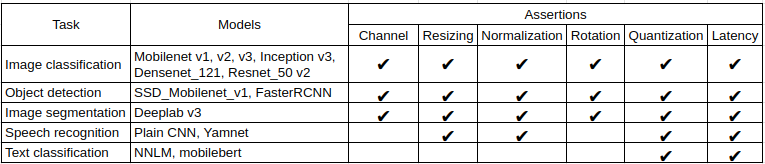
Figure 3: Summary of tasks, models and assertions in our evaluation. ML-EXray applies to a wide range of tasks and can identify deployment issues across multiple dimensions including input processing, quantization, and system performance such as abnormal latency.

We evaluate ML-EXray by deploying various ML-based applications on mobile devices, referring to public deployment tutorials and open-source application repositories. To examine the efficacy of ML-EXray, we instrument these applications using ML-EXray APIs, and catch deployment issues by evaluating built-in as well as custom assertions. Our evaluation is designed to support the following claims:

* ML-EXray catches a wide range of edge deployment issues in industrial production systems across different ML applications. Using ML applications of different sensor modalities (e.g., image, audio, text), we show that ML-EXray can quickly identify a variety of input preprocessing bugs in the inference pipeline (§4.3), quantization issues of the model (§4.4), and latency issues due to sub-optimal operations on target hardware (§4.5).

* ML-EXray is lightweight and easy to use. We measure the efficiency and system overhead that ML-EXray incurs, e.g., extra latency, memory usage, etc. We also show that ML-EXray significantly reduced the line-of-code (LoC) needed to catch deployment issues, lowering the barrier for debugging and demonstrating its capability of providing visibility into the deployment process.

* ML-EXray improves app performance. We quantify the impact of the identified deployment issues for various ML applications. Our evaluations show that, just by eradicating these issues found by assertions of a few LoC, ML-EXray can improve model performance on the edge by a significant margin. The evaluation raises awareness of these problems, and ML-EXray offers a systematic solution.

Specifically, we write and deploy widely-used ML applications in everyday life, such as image classification (automated grocery store), object detection (surveillance, security camera), segmentation (autonomous driving), speech recognition (home assistant), text classification (sentiment analysis), etc. For each task, we use one or more off-the-shelf pretrained models, such as different versions of MobileNet Howard et al. (2017), Densenet Huang et al. (2017), SSD Liu et al. (2016), Deeplab Chen et al. (2017), MobileBert Sun et al. (2020). To evaluate ML-EXray, we deploy these apps on a Pixel 4 and Pixel 3 with 64-bit octa-core CPU (2.84GHz, 2.5GHz), and mobile GPUs (Adreno 640, 630). To benchmark performance, these apps are instrumented, using our APIs, in a way that they can accept data from an SD card in addition to the original sensor streams. We use standard task-specific datasets (e.g., ImageNet Deng et al. (2009), COCO Lin et al. (2014), speech commands Warden (2018) for the evaluation.

Our reference pipelines are adapted from the original training pipelines source code of each of the models evaluated. We run the reference pipelines on a workstation with a 2.2 GHz Intel Core i7 6-Core CPU and a GeForce 3070 GPU.

4.1 ML-EXray can Identify a Wide Range of Deployment Issues across Various Tasks

Figure 3 shows a summary of our evaluation. As shown in the figure, ML-EXray is generic and can be applied to a variety of different models of different tasks for edge deployment. These tasks range from image-based, to audio- and text-based applications. The architecture of models varies from convolutional neural networks Howard et al. (2017) to language embeddings Bengio et al. (2003) and transformers Devlin et al. (2018); Dosovitskiy et al. (2020). The instrumentation and logging using ML-EXray APIs are universal around different models and their edge inference pipelines. Some of the assertions such as quantization validation and system metrics check (such as latency and memory usage) are also task and model agnostic. When it comes to task-specific assertions, for example, image preprocessing assertions, they are applicable to a range of tasks, such as classification, detection, segmentation, pose estimation, etc. These preprocessing assertions include, but are not limited to, the following (see details in §2): validating channel extraction, resizing functions, normalization scale, as well as input orientation. A few of them, such as normalization and resizing function validation, are also applicable to other input modalities of multi-dimensional arrays, such as audio spectrograms. Our evaluation shows that ML-EXray is capable of catching these issues among all these different applications. In the following sections, we show that ML-EXray is easy to use (§4.2). Also, we detail the issues we found on some of these deployed inference pipelines, and quantify their impact (§4.3, §4.4, §4.5)

4.2 ML-EXray is Light and Easy to Use

In this section, we quantify the overhead of using ML-EXray to validate edge deployment. There are three steps that incur overhead: 1) app instrumentation and writing assertion functions, 2) extra run-time latency, memory, and storage, and 3) offline validation procedures and assertions.

App instrumentation and assertion functions. Without ML-EXray, app developers have to write a significant chunk of code to get the inference logs and compose assertion functions. Table 1 shows how much easier it is to use ML-EXray for both instrumentations as well as assertions, compared to writing everything from scratch. Extracting and asserting output from custom preprocessing functions is easier (25 LoC), ML-EXray abstracts these to under 5 LoC. It is harder to check and validate per-layer details. For example, asserting per-layer output can verify the correctness of model optimization and quantization, per-layer latency can verify the efficiency of optimized operation on different hardware. ML-EXray abstracts per-layer logging, log parsing, and per-layer metric comparisons, of which the code can easily go over 100 LoC. With ML-EXray, users only need up to 15 LoC to scrutinize per-layer details.

	Line of Code
Debugging	W/ ML-EXray			W/O ML-EXray
Target	Inst	Asrt	Total	Inst	Asrt	Total
Preprocessing	1	3	4	18	7	25
Quantization	4	9	13	82	183	265
Lat. & Mem.	4	4	8	14	8	22
Per-layer Lat.	2	6	8	14	90	104

Table 1: Line-of-code (LoC) of instrumentation and assertion to write for each debugging target. With ML-EXray APIs, app instrumentation can be cut down to less than 5 LoC. The ML-EXray assertion interface abstracts away log parsing, making assertions functions simpler and easier to write.

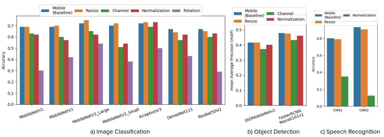
Figure 4: ML application performance across three different tasks degraded by preprocessing bugs found in industry deployment: erroneous channel arrangement, different resizing functions, mismatching normalization scale, and disoriented input.

App run-time overhead. We next ask how much overhead ML-EXray incurs during app run-time. Table 2 shows the latency, memory, and storage needed to run an instrumented app with ML-EXray. We instrumented and deployed an image classification app on Android Phones. The app runs MobileNet v2 over 100 images from the ImageNet test split. By default, we use 4 threads to run the ML model. As shown in Table 2, ML-EXray run-time logging only incurs up to 3 ms (15%) latency when using Adreno mobile GPUs. Latency overhead is negligible (2.3%) when using CPU. It also consumes about 3.7MB memory. Run-time logs are saved on an SDcard, and are as small as 0.41 KB per frame.

	Lat (ms)	Lat (ms)	Mem	Disk
	CPU only	GPU enabled	(MB)	(KB/Frm)
Pixel 4	128.2±6.1	16.7±0.3	6.42	-
P4(Inst)	129.6±5.0	19.1±0.6	10.12	0.41
Pixel 3	157.0±6.7	28.4±0.4	9.26	-
P3(Inst)	158.3±7.3	30.0±0.5	12.37	0.41

Table 2: Run-time instrumentation overhead: latency, memory, and external storage. Numbers are from deploying an image classification app using Mobilenet v2 on Pixel 4 and Pixel 3 phones.

Validation and assertion overhead. As shown in the debugging flow chart Figure 2, when ML-EXray finds an indication of deployment issues (e.g., accuracy degradation) from the run-time logs, it triggers a fine-grained offline validation. This step involves logging per-layer output from both the edge and the reference pipeline. Depending on the complexity of the model deployed, the log size and the latency can vary a lot. To show the difference, we pick models with increasing layers (from 92 to 429) and the number of parameters of different magnitudes (from 3.5M to 25M).

	Layer	Param	Lat	Mem	Disk
	#	#	(sec)	(MB)	(MB)
Mobilenet v1	92	4.2M	14	2	44
Mobilenet v2	156	3.5M	16	1	51
Resnet50 v2	192	25.6M	67	24	176
Inception v3	313	23.9M	57	46	150
Densenet 121	429	8M	70	74	177

Table 3: Offline validation overhead: latency, memory, and external storage (quantized 8-bit integer model).

Table 3 shows the latency, memory and storage space needed for these models, in the quantized 8-bit integer version (see Table 5 in appendix for 32-bit float version). The evaluation shows that logging per-layer details can incur 14 to over 100 seconds (linear to model complexity) on edge devices (e.g., Pixel 4). The memory footprint of these models varies from a few to hundreds of MB. The per-layer logs range from 44 MB to over 400 MB. The logs from the reference pipelines of the same model are of the same magnitude. Fortunately, comparing these two logs takes only a few seconds on commodity workstations, which is negligible given the logging latency (two orders of magnitude longer).

4.3 Preprocessing Bugs and Impact

ML applications usually involve a few standard, yet error-prone, preprocessing steps for sensor input (§2), including, but not limited to, channel extraction, resizing, numerical conversion, and orientation. ML-EXray catches bugs in these functions by comparing the output of these functions to correct reference processing pipelines using user-defined assertions. To benchmark the impact of these bugs, we instrument Android ML apps to take input data from external storage instead of sensor streams, and run the app over publicly available task-specific benchmark datasets.

Figure 4 (a) shows the image classification accuracy of various models when one erroneous preprocessing function is applied. These preprocessing bugs, ranked by the severity of impact on Top-1 accuracy, include using 1) a different resizing function (Resize, orange), 2) an erroneous channel arrangement (Channel, green), 3) a mismatching normalization scale (Normalization, red), and 4) a disoriented input (Rotation, purple). For all models, the baseline (optimized 32-bit float model, denoted as Mobile, blue) always uses the same preprocessing functions from their training pipeline (e.g., resizing using area averaging, arranging channel order as RGB, normalizing input to [-1.0,1.0], and using the original image orientation for Mobilenet v2). Each bar independently introduces one and only one erroneous preprocessing function without inheriting from other bars.

Compared to the baseline: a) using a different resizing function in the inference pipeline (e.g., bilinear resampling vs. area averaging), the Top-1 accuracy can vary by 1-3%; b) using a different channel arrangement order (e.g., RGB vs. BGR), the model accuracy can degrade by 7-19%, depending on how much the models care about the structural features versus the absolute pixel values; c) using a different normalization scale (e.g., [0.0,1.0] vs. [-1.0,1.0]), the model accuracy can drop by up to 20% easily; d) rotating the image by 90 degrees (to emulate a disoriented image captured from mobile devices) can immediately break the app with the most severe 21-39% accuracy drop, even though most of these models are trained with data augmentations Shorten & Khoshgoftaar (2019), such as random rotation and flipping.

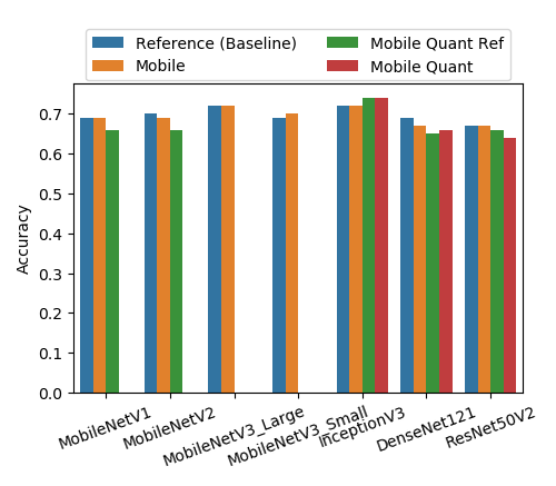
Figure 5: Model top-1 accuracy affected by optimization and quantization.

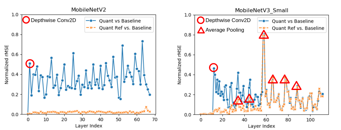
Figure 6: Normalized root-mean-square-error (rMSE) between quantized model vs. reference baseline for MobileNet v2 and v3.

Other tasks. We also evaluate the impact of preprocessing bugs on other ML applications, including object detection, segmentation, speech recognition, and text classification, etc. Intuitively, the preprocessing bugs can affect other image-based applications. Figure 4 (b) shows an example of degraded mean average precision of object detection models on COCO Lin et al. (2014) validation set for SSD Liu et al. (2016) and FasterRCNN Ren et al. (2015). Channel misarrangement and erroneous normalization can lower mAP by up to 4%, while a different resizing function changes mAP by only 0.1%. Preprocessing bugs can also impact tasks of different sensor modalities. Figure 4 (c) shows lower audio recognition accuracy on a speech command dataset Warden (2018). In Figure 4, we use two speech models from different training pipelines spe . Mismatching spectrogram normalization can significantly hurt these speech models. We have also evaluated segmentation and text sentiment classification tasks, where the impact of these preprocessing bugs is less significant (see Appendix §A).

4.4 Quantization Issues and Impact

In order to validate model optimization and quantization, we leverage the per-layer details from ML-EXray logs. In addition to verifying the performance of the optimized model against the original one, ML-EXray also scrutinizes, layer by layer, to identify small output drifts or huge discrepancies. The former of which indicates arithmetic resolution issues, while the latter indicates incorrect operations.

Figure 6 shows the image classification accuracy of various models in increasingly optimized versions during the deployment process. For each model, here the baseline (Reference, blue) is the original checkpoint format from the training pipeline. The other bars represent 1) an optimized 32-bit float model (Mobile, orange), 2) a quantized 8-bit integer model using OpResolver OpR (Mobile Quant, red), a built-in operation resolver that invokes an “optimized kernel” for production, and 3) the same fully quantized 8-bit integer model using RefOpResolver Ref (Mobile Quant Ref, green), a built-in reference operation resolver that invokes a “reference kernel” for debugging (to rule out the possibility of issues caused by optimization). Optimization for OpResolver could cause small discrepancies on float models due to the non-associativity of floating point arithmetic. So any accuracy discrepancies in int8 fully-quantized model between builtin op and builtin reference op should be treated as a bug, which could mainly come from different overflow behavior in the optimized kernel and the reference kernel. From a user perspective, the major difference between RefOpResolver and OpResolver is execution speed, and ML-EXray can leverage the two OpResolvers to provide debugging insights. Beyond the two built-in op resolvers, advanced users have the option to create their own OpResolver which could invoke their custom ops and kernels, which may or may not deviate from built-in behaviors.

We now summarize the results and dive deeper into the root causes. Compared to the baseline: a) even without any quantization, running the converted 32-bit float model on mobile phones can already have a 1-2% accuracy drop (Baseline vs. Mobile) (in that the specific arithmetic operations are not entirely the same), b) correctly executed quantized models using RefOpResolver can further incur $\pm 3\%$ accuracy change for MobileNet v1, v2, Inception v3, and Resnet 50 v2 (Mobile vs. Mobile Quant Ref). However, it can result in 0% accuracy (MobileNetv3) with invalid or constant output. In cases where RefOpResolver does not have a significant accuracy drop (e.g., MobileNet v1, v2), quantized models using optimized kernel can be error-prone to specific operations, yielding invalid or constant output (Mobile Quant Ref vs. Mobile Quant).

To reason about getting 0% accuracy from quantized models on MobileNet (Figure 6), we show the per-layer diagnosis result of two examples (v2 and v3) that reveal different issues (b) and c) above. Figure 6 depicts the normalized rMSE of each layer output when comparing Mobile Quant (blue), and Mobile Quant Ref (orange) against the baseline. The numbers are drawn from running a MobileNet v2 (left) and v3 (right) model on a Pixel 4.

In the case of v2, using RefOpResolver, the $\widehat{rMSE}$ is always below 10%, which explains the 1-3% accuracy drop. However, the quantized model using the built-in op resolver shows a jump of rMSE at the second layer (red circle) of MobileNet v2 (also the 13th layer of v3). Further inspection of the model architecture reveals that these are DepthwiseConv2D layers, which indicates that the optimized op resolver has a bug on the depthwise convolution op.

Ruling out the factor of the op resolver, we take another look at the case of Mobile Quant Ref on MobileNet v3, which, despite the correct execution of depthwise convolution, still has 0% accuracy. The right figure of Figure 6 shows that the normalized rMSE is having several peaks (red triangles) at layer 33, 44, 57, 64, 77, 87, etc. These peaks respond to the average pooling layer, which is an addition from v2 to v3, in each residual block.

At this point, ML-EXray can confidently report the error-prone layers and direct the user to further inspect the op implementation of these layers. In fact, ML-EXray is the first to uncover these two issues. Thanks to ML-EXray, they are now under the radar of the Tensorflow developers.

4.5 Sub-optimal Kernels and Latency

Depending on run-time optimization, ML operations executed on different platforms can have drastically different latency. For example, although reference op resolver may guarantee a correct execution, it can incur over 200$\times$ longer latency on mobile devices. Table 4 summarizes ML-EXray total per-layer latency by layer type of MobileNetv2.

Layer	Mobile	Mobile	Mobile	Emulator(x86)
Type		Quant	Quant	Mobile
(Count)	(ms)	(ms)	Ref (ms)	(ms)
D-Conv(17)	95.4	22.7	2885.2	120.0
Conv(35)	23.5	32.3	18662.3	1409.8
FC(1)	7.4	7.1	7.0	71.2
Mean(1)	6.1	5.6	5.0	2.5
Pad(4)	1.6	18.7	60.8	104.8
Add(10)	1.5	7.7	99.8	7.0
Softmax(1)	0.4	0.0	0.0	0.2
Quantize(1)	-	3.3	0.7	-
Total	136.26	97.816	21721.2	1715.7

Table 4: Latency by layer type of MobileNetv2 executed on Pixel 4 and android emulator for Pixel 4.

The latency differences of each layer type are very interesting. a) Quantized 2D convolution layer is slower than the unquantized one using optimized op resolver. b) Each depth-wise 2D convolution is 8$\times$ heavier than normal 2D convolution layer on 32-bit float model, whereas quantized depthwise convolution is faster than normal convolution layer. c) Unoptimized reference op resolve is three orders of magnitude slower than the optimized one: it significantly slows down convolution, depth-wise convolution, padding and addition. d) operations are ARM-specific, which cannot benefit on x86 emulators. The 32-bit float model on an emulator has comparable depth-wise convolution layer latency, but is 44x slower on normal convolution layers. It remains a challenge to faithfully emulate edge device performance metrics on platforms with more compute but different architecture, because op optimizations are architecture-specific.

5 Related Work

ML inference at the edge. Recent years have seen growing demand for running ML applications with latency, bandwidth, and privacy constraints on edge devices. These edge devices are equipped with special low-power hardware (e.g., Qualcomm Adreno GPUs adr , Coral edge TPUs edg , Intel VPUs vpu , micro-controllers ard and DSPs). To push ML to the edge, the research and industry community have put significant effort (e.g., TinyML Warden & Situnayake (2019), Tflite Lee et al. (2019), TfliteMicro David et al. (2021), PyTorchMobile tor ) in optimizing the ML execution on these heterogeneous hardware devices.

ML profiling and benchmarks. Previous work has focused on profiling ML training Mattson et al. (2019), inference performance Reddi et al. (2020a) in the cloud Wang et al. (2020). Recent work looks at profiling kernel operations (DeepBench dee ) of different ML frameworks Luo et al. (2020) with respect to different hardware Tang et al. (2021); Zhang et al. (2021); Tao et al. (2017) at the edge. However, there is very little work on validating and debugging the deployment process.

ML Validation. Recent work raises the awareness of model performance validation by introducing model assertions Kang et al. (2018) to check inconsistent outputs from models, or being run across different devices Cidon et al. (2021). Our work looks beyond the output and provides visibility inside the model, and focuses on the system issues of edge deployment Paleyes et al. (2021).

6 Conclusion

In this work, we introduce ML-EXray, a validation framework for edge ML deployment. ML-EXray enables app developers to catch complicated deployment issues just by writing a few lines of instrumentation and assertion code. We implemented ML-EXray as a suite of multi-lingual instrumentation APIs and an end-to-end deployment validation library, which will be open-sourced. Using different ML models for image, audio, and text-based applications, we showed that ML-EXray can help catch a variety of issues including preprocessing bugs, model optimization and quantization issues, and suboptimal kernel execution. Eradicating these issues can substantially improve edge application accuracy and latency. Code and APIs will be open-sourced to the community as a multi-lingual instrumentation library and a Python deployment validation library.

Appendix A Addtional Evaluation Results

Deployment issues and impact on other tasks. In addition to image classification, object detection, and speech recognition shown in §4, we have also deployed a text sentiment classification app using MobileBert Sun et al. (2020), and NNLM embeddings Bengio et al. (2003) as well as image segmentation apps using Deeplab v3 Chen et al. (2017). We observe that even per-layer output values can be different in these models, the output accuracy is not significantly changed. For example, when NNLM takes raw texts versus the same text but with lower case, the embedding output is drastically different. However, the sentiment classification accuracy on the IMDB movie review dataset Maas et al. (2011) is exactly the same. Further, some models, such as EfficientDet Tan et al. (2020), incorporate the input preprocessing functions into the model graph, which reduces the chance of having preprocessing bugs during deployment.

Offline validation overhead. We show the offline validation overhead (Table 5) for floating-point models. This is in correspondence to Table 3 in §4.2

	Layer	Param	Lat	Mem	Disk
	#	#	(sec)	(MB)	(MB)
Mobilenet v1	92	4.2M	21	53	87
Mobilenet v2	156	3.5M	21	6	93
Resnet50 v2	192	25.6M	104	60	478
Inception v3	313	23.9M	85	155	333
Densenet 121	429	8M	114	298	426

Table 5: Offline validation overhead: latency, memory, and external storage (original 32 bit float model).

Appendix B Additional Design Details

Figure 7 shows a system diagram. A general workflow is as follows. Both the instrumented mobile app (§3.2) and the reference pipelines (§3.3) will instantiate the EdgeML Monitor (§3.2) to collect telemetry data of ML inferences. ML-EXray uses these data to compare and validate the mobile ML pipeline against the reference pipeline (§3.4). For well-defined tasks, such as image classification, object detection, audio recognition, ML-EXray provides built-in assertions on critical error-prone points (e.g., preprocessing) where bugs are common.

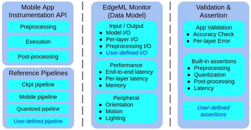
Figure 7: ML-EXray system diagram. ML-EXray includes app intrumentation APIs (§3.2), reference ML inference pipelines (§3.3), and deployment validation framework (§3.4). Both the APIs and reference pipelines use an underlying EdgeML Monitor to log ML inference traces for validation and assertion. Users can customize logs and assertion functions, and provide user-defined pipelines as reference baselines.

To invoke ML-EXray in Java, users can write:

⬇

MLEXray.on_inf_start();

// invoke tflite...

MLEXray.on_inf_stop();

To log the peripheral sensors during the camera shuttering, the developer may write (in Java):

⬇

void onImageAvailable(ImageReader reader) {

MLEXray.on_sensor_stop();

// process image ...

MLEXray.on_sensor_start();}

References

- (1) Tensorflow lite built-in op resolver. URL https://github.com/tensorflow/tensorflow/blob/master/tensorflow/lite/kernels/register.h.
- (2) Tensorflow lite built-in reference op resolver. URL https://github.com/tensorflow/tensorflow/blob/master/tensorflow/lite/kernels/register_ref.h.
- (3) Qualcomm adreno mobile gpu. URL https://www.qualcomm.com/products/features/adreno.
- (4) Arduino platform. URL https://www.arduino.cc/.
- (5) Benchmarking deep learning operations on different hardware. URL https://github.com/baidu-research/DeepBench.
- (6) Intel vpu. URL https://cloud.google.com/edge-tpu.
- (7) Tensorflow keras application module: tf.keras.applications. URL https://www.tensorflow.org/api_docs/python/tf/keras/applications.
- (8) Simple audio recognition tutorial. URL https://www.tensorflow.org/tutorials/audio/simple_audio.
- (9) Tensorflow model optimization. URL https://www.tensorflow.org/model_optimization/guide.
- (10) Pytorch mobile. URL https://pytorch.org/mobile/.
- (11) Intel vpu. URL https://www.intel.com/content/www/us/en/products/details/processors/movidius-vpu.html.
- (12) Yamnet: a speech recognition model. URL https://tfhub.dev/google/yamnet/1.
- Bengio et al. (2003) Bengio, Y., Ducharme, R., Vincent, P., and Janvin, C. A neural probabilistic language model. The journal of machine learning research, 3:1137–1155, 2003.
- Chen et al. (2017) Chen, L.-C., Papandreou, G., Kokkinos, I., Murphy, K., and Yuille, A. L. Deeplab: Semantic image segmentation with deep convolutional nets, atrous convolution, and fully connected crfs. IEEE transactions on pattern analysis and machine intelligence, 40(4):834–848, 2017.
- Cidon et al. (2021) Cidon, E., Pergament, E., Asgar, Z., Cidon, A., and Katti, S. Characterizing and taming model instability across edge devices. In Smola, A., Dimakis, A., and Stoica, I. (eds.), Proceedings of Machine Learning and Systems, volume 3, pp. 624–636, 2021. URL https://proceedings.mlsys.org/paper/2021/file/b53b3a3d6ab90ce0268229151c9bde11-Paper.pdf.
- David et al. (2021) David, R., Duke, J., Jain, A., Janapa Reddi, V., Jeffries, N., Li, J., Kreeger, N., Nappier, I., Natraj, M., Wang, T., Warden, P., and Rhodes, R. Tensorflow lite micro: Embedded machine learning for tinyml systems, 2021.
- Deng et al. (2009) Deng, J., Dong, W., Socher, R., Li, L.-J., Li, K., and Fei-Fei, L. Imagenet: A large-scale hierarchical image database. In 2009 IEEE Conference on Computer Vision and Pattern Recognition, pp. 248–255, 2009. doi: 10.1109/CVPR.2009.5206848.
- Devlin et al. (2018) Devlin, J., Chang, M.-W., Lee, K., and Toutanova, K. Bert: Pre-training of deep bidirectional transformers for language understanding. arXiv preprint arXiv:1810.04805, 2018.
- Dosovitskiy et al. (2020) Dosovitskiy, A., Beyer, L., Kolesnikov, A., Weissenborn, D., Zhai, X., Unterthiner, T., Dehghani, M., Minderer, M., Heigold, G., Gelly, S., et al. An image is worth 16x16 words: Transformers for image recognition at scale. arXiv preprint arXiv:2010.11929, 2020.
- Han et al. (2016) Han, S., Mao, H., and Dally, W. J. Deep compression: Compressing deep neural networks with pruning, trained quantization and huffman coding, 2016.
- Howard et al. (2017) Howard, A. G., Zhu, M., Chen, B., Kalenichenko, D., Wang, W., Weyand, T., Andreetto, M., and Adam, H. Mobilenets: Efficient convolutional neural networks for mobile vision applications. arXiv preprint arXiv:1704.04861, 2017.
- Huang et al. (2017) Huang, G., Liu, Z., Van Der Maaten, L., and Weinberger, K. Q. Densely connected convolutional networks. In 2017 IEEE Conference on Computer Vision and Pattern Recognition (CVPR), pp. 2261–2269, 2017. doi: 10.1109/CVPR.2017.243.
- Jacob et al. (2017) Jacob, B., Kligys, S., Chen, B., Zhu, M., Tang, M., Howard, A., Adam, H., and Kalenichenko, D. Quantization and training of neural networks for efficient integer-arithmetic-only inference, 2017.
- Kang et al. (2018) Kang, D., Raghavan, D., Bailis, P., and Zaharia, M. Model assertions for debugging machine learning. In NeurIPS MLSys Workshop, 2018.
- Krishnamoorthi (2018) Krishnamoorthi, R. Quantizing deep convolutional networks for efficient inference: A whitepaper. arXiv preprint arXiv:1806.08342, 2018.
- Lee et al. (2019) Lee, J., Chirkov, N., Ignasheva, E., Pisarchyk, Y., Shieh, M., Riccardi, F., Sarokin, R., Kulik, A., and Grundmann, M. On-device neural net inference with mobile gpus, 2019.
- Li & Alvarez (2021) Li, J. and Alvarez, R. On the quantization of recurrent neural networks. arXiv preprint arXiv:2101.05453, 2021.
- Lin et al. (2014) Lin, T.-Y., Maire, M., Belongie, S., Hays, J., Perona, P., Ramanan, D., Dollár, P., and Zitnick, C. L. Microsoft coco: Common objects in context. In European conference on computer vision, pp. 740–755. Springer, 2014.
- Liu et al. (2016) Liu, W., Anguelov, D., Erhan, D., Szegedy, C., Reed, S., Fu, C.-Y., and Berg, A. C. Ssd: Single shot multibox detector. In European conference on computer vision, pp. 21–37. Springer, 2016.
- Luo et al. (2020) Luo, C., He, X., Zhan, J., Wang, L., Gao, W., and Dai, J. Comparison and benchmarking of ai models and frameworks on mobile devices, 2020.
- Maas et al. (2011) Maas, A. L., Daly, R. E., Pham, P. T., Huang, D., Ng, A. Y., and Potts, C. Learning word vectors for sentiment analysis. In Proceedings of the 49th Annual Meeting of the Association for Computational Linguistics: Human Language Technologies, pp. 142–150, Portland, Oregon, USA, June 2011. Association for Computational Linguistics. URL http://www.aclweb.org/anthology/P11-1015.
- Mattson et al. (2019) Mattson, P., Cheng, C., Coleman, C., Diamos, G., Micikevicius, P., Patterson, D., Tang, H., Wei, G.-Y., Bailis, P., Bittorf, V., et al. Mlperf training benchmark. arXiv preprint arXiv:1910.01500, 2019.
- Nagel et al. (2021) Nagel, M., Fournarakis, M., Amjad, R. A., Bondarenko, Y., van Baalen, M., and Blankevoort, T. A white paper on neural network quantization, 2021.
- Paleyes et al. (2021) Paleyes, A., Urma, R.-G., and Lawrence, N. D. Challenges in deploying machine learning: a survey of case studies, 2021.
- Reddi et al. (2020a) Reddi, V. J., Cheng, C., Kanter, D., Mattson, P., Schmuelling, G., Wu, C.-J., Anderson, B., Breughe, M., Charlebois, M., Chou, W., et al. Mlperf inference benchmark. In 2020 ACM/IEEE 47th Annual International Symposium on Computer Architecture (ISCA), pp. 446–459. IEEE, 2020a.
- Reddi et al. (2020b) Reddi, V. J., Kanter, D., Mattson, P., Duke, J., Nguyen, T., Chukka, R., Shiring, K., Tan, K.-S., Charlebois, M., Chou, W., et al. Mlperf mobile inference benchmark. arXiv preprint arXiv:2012.02328, 2020b.
- Ren et al. (2015) Ren, S., He, K., Girshick, R., and Sun, J. Faster r-cnn: Towards real-time object detection with region proposal networks. Advances in neural information processing systems, 28:91–99, 2015.
- Savsunenko (2018) Savsunenko, O. How tensorflow’s tf.image.resize stole 60 days of my life, 2018. URL https://medium.com/hackernoon/how-tensorflows-tf-image-resize-stole-60-days-of-my-life-aba5eb093f35.
- Shangguan et al. (2019) Shangguan, Y., Li, J., Liang, Q., Alvarez, R., and McGraw, I. Optimizing speech recognition for the edge. arXiv preprint arXiv:1909.12408, 2019.
- Shorten & Khoshgoftaar (2019) Shorten, C. and Khoshgoftaar, T. M. A survey on image data augmentation for deep learning. Journal of Big Data, 6(1):1–48, 2019.
- Simonyan & Zisserman (2014) Simonyan, K. and Zisserman, A. Very deep convolutional networks for large-scale image recognition. arXiv preprint arXiv:1409.1556, 2014.
- Sun et al. (2020) Sun, Z., Yu, H., Song, X., Liu, R., Yang, Y., and Zhou, D. Mobilebert: a compact task-agnostic bert for resource-limited devices. arXiv preprint arXiv:2004.02984, 2020.
- Tan et al. (2020) Tan, M., Pang, R., and Le, Q. V. Efficientdet: Scalable and efficient object detection, 2020.
- Tang et al. (2021) Tang, X., Han, S., Zhang, L. L., Cao, T., and Liu, Y. To bridge neural network design and real-world performance: A behaviour study for neural networks. In Smola, A., Dimakis, A., and Stoica, I. (eds.), Proceedings of Machine Learning and Systems, volume 3, pp. 21–37, 2021.
- Tao et al. (2017) Tao, J., Du, Z., Guo, Q., Lan, H., Zhang, L., Zhou, S., Xu, L., Liu, C., Liu, H., Tang, S., Rush, A., Chen, W., Liu, S., Chen, Y., and Chen, T. Benchip: Benchmarking intelligence processors, 2017.
- Wallace (1992) Wallace, G. K. The jpeg still picture compression standard. IEEE transactions on consumer electronics, 38(1):xviii–xxxiv, 1992.
- Wang et al. (2020) Wang, Y. E., Wei, G.-Y., and Brooks, D. A systematic methodology for analysis of deep learning hardware and software platforms. In The 3rd Conference on Machine Learning and Systems (MLSys), 2020.
- Warden (2018) Warden, P. Speech Commands: A Dataset for Limited-Vocabulary Speech Recognition. ArXiv e-prints, April 2018. URL https://arxiv.org/abs/1804.03209.
- Warden & Situnayake (2019) Warden, P. and Situnayake, D. Tinyml: Machine learning with tensorflow lite on arduino and ultra-low-power microcontrollers. O’Reilly Media, 2019.
- Zhang et al. (2021) Zhang, L., Han, S., Wei, J., Zheng, N., Cao, T., Yang, Y., and Liu, Y. nn-meter: towards accurate latency prediction of deep-learning model inference on diverse edge devices. In 2021 International Conference on Mobile Systems, Applications, and Services, pp. 81–93. ACM, June 2021.
- Zhou & Tuzel (2018) Zhou, Y. and Tuzel, O. Voxelnet: End-to-end learning for point cloud based 3d object detection. In Proceedings of the IEEE conference on computer vision and pattern recognition, pp. 4490–4499, 2018.