Coupled-channel analysis of pion- and eta-electroproduction with the Jülich-Bonn-Washington model

Abstract

Pion and eta electroproduction data are jointly analyzed for the first time, up to a center-of-mass energy of 1.6 GeV. The framework is a dynamical coupled-channel model, based on the recent Jülich-Bonn-Washington analysis of pion electroproduction data for the same energy range. Comparisons are made to a number of single-channel eta electroproduction fits. By comparing multipoles of comparable fit quality, we find some of these amplitudes are well determined over the near-threshold region, while others will require fits over an extended energy range.

I Introduction

Early progress in baryon spectroscopy was driven by the analysis of meson-nucleon scattering data, such as pion-nucleon scattering ($\pi N\to\pi N$, $\pi N\to\pi\pi N$); see, e.g., Refs Höhler (1983); Cutkosky et al. (1979); Arndt et al. (2006, 2009); Shrestha and Manley (2012). A viable alternative to this, specifically advantageous for detecting unstable intermediate states with small branching ratios to the $\pi N$ channel, are photon-induced reactions Ireland et al. (2020). Large data bases have been accumulated for these reactions as part of the extensive experimental programs at Jefferson Laboratory, MAMI, ELSA and other facilities Aznauryan et al. (2009); Achenbach et al. (2017); Carman et al. (2020); Beck and Thoma (2017); Shiu et al. (2018); Akondi et al. (2019); Ho et al. (2018); Ohnishi et al. (2020); Alef et al. (2020); Zachariou et al. (2021); Shrestha et al. (2021); Markov et al. (2020).

On the theory side, many approaches have been developed to describe these reactions. Specifically for pion electroproduction, chiral perturbation theory (ChPT) has been successfully applied in the analysis of the threshold region Bernard et al. (1992, 1993, 1994, 1996); Hilt et al. (2013). In building on ChPT, chiral unitary models (see, e.g., the recent review Mai (2021)) have also become quite successful in accessing the resonance region. Such models provide the hadronic structure of many gauge-invariant chiral unitary formalisms Ruić et al. (2011); Mai et al. (2012); Bruns (2020); Döring and Nakayama (2010a, b); Borasoy et al. (2007); Meißner and Oller (2000). For an in-depth discussion of the manifest implementation of gauge invariance see Ref. Haberzettl (2021). For even larger kinematical ranges, and large data bases, many phenomenological models have been developed. Major classes of those are: (1) isobar models Chiang et al. (2002); Aznauryan (2003); Drechsel et al. (2007); Tiator et al. (2018) with unitarity constraints at lower energies; (2) $K$-matrix-based formalisms with built-in cuts associated with opening inelastic channels, and dispersion-relation constraints Aznauryan (2003); Hanstein et al. (1998); Workman et al. (2012). Multi-channel analyses have analyzed data and, in some cases, amplitudes from hadronic scattering data together with the photon-induced channels Briscoe et al. (2015) by the Gießen Shklyar et al. (2007), Bonn-Gatchina Anisovich et al. (2012a), Kent State Shrestha and Manley (2012), ANL-Osaka Kamano et al. (2013), Jülich-Bonn (JüBo) Rönchen et al. (2015) and JPAC Nys et al. (2017) groups. For more details, see the introduction of our recent paper Mai et al. (2021).

Dynamical coupled-channel approaches Rönchen et al. (2018); Kamano et al. (2016); Rönchen et al. (2015); Kamano et al. (2013); Rönchen et al. (2014); Kamano et al. (2010); Tiator et al. (2010) (DCC) have led to the discovery and confirmation of many new states Zyla et al. (2020) by extracting universal resonance parameters in terms of pole positions and residues of the transition amplitude in the complex-energy plane. In many analyses of pion- and photon-induced reactions, mass scans and $\chi^{2}$ arguments are used to identify new states Crede et al. (2011); Anisovich et al. (2017) but recently model selection has also been explored Landay et al. (2019, 2017).

Furthermore, by extracting Drechsel et al. (1999); Arndt et al. (2002); Chiang et al. (2002); Tiator et al. (2003, 2004); Aznauryan et al. (2005a, b); Corthals et al. (2007); Drechsel et al. (2007); Aznauryan et al. (2009); Aznauryan and Burkert (2012a); Tiator et al. (2011); Aznauryan et al. (2013); Vrancx et al. (2014); Maxwell (2014); Mokeev et al. (2016); Isupov et al. (2017); Burkert et al. (2019); Hiller Blin et al. (2019); Mart et al. (2002); Mokeev et al. (2020) the $Q^{2}$ dependence of resonance couplings, a link between perturbative QCD and the region where quark confinement sets in can be established that serve as point of comparison for many quark models Isgur and Karl (1978); Capstick and Isgur (1985); Capstick (1992); Capstick and Roberts (1994); Ronniger and Metsch (2011); Ramalho and Pena (2011); Jayalath et al. (2011); Aznauryan and Burkert (2012b); Golli and Širca (2013); Obukhovsky et al. (2019); Ramalho et al. (2020); Ramalho and Peña (2020) and Dyson-Schwinger equations Roberts and Williams (1994); Roberts (2008); Eichmann et al. (2010); Wilson et al. (2012); Chen et al. (2012); Eichmann and Fischer (2013); Xu et al. (2015); Segovia et al. (2015); Eichmann et al. (2016a, b); Burkert and Roberts (2019); Chen et al. (2019a); Qin et al. (2018, 2019); Chen et al. (2019b); Lu et al. (2019).

However, so far, no unified coupled-channel analysis of photo- and electroproduction experiments exists that simultaneously describes the $\pi N$, $\eta N$ and $K\Lambda$ final states. The present study provides a first step in this direction in the form of a coupled-channel analysis of pion and eta electroproduction data, extending our recent analysis of pion electroproduction data Mai et al. (2021). It is based on the JüBo approach Rönchen et al. (2015) which fits an extensive scattering and photoproduction data base in the resonance region.

This study is organized as follows. Section II outlines formal aspects of the Jülich-Bonn-Washington (JBW) approach to pseudo-scalar meson electroproduction. These include the generalization to electroproduction of different final states and the influence of kinematic limits ($Q^{2}=0$, thresholds for channel openings, and pseudo-thresholds associated with Siegert’s theorem Siegert (1937); Tiator (2016)). Furthermore, we define the parametrization of the $Q^{2}$ dependence from the photon point at $Q^{2}=0$, where the underlying JüBo model describes photon- and meson-induced reactions, to electroproduction.

Section III reviews the results of previous single-channel fits to eta electroproduction data. Section IV describes the data used in our fits, strategies to find $\chi^{2}$ minima, and a modified $\chi^{2}$ which more evenly weights the contributions of observables with different abundances. Section V compares our fits to data. Eta electroproduction multipoles are also compared, with etaMAID results displayed for reference.

Section VI compares the single- and coupled-channel results, with qualitative features discussed based on data quality/consistency. Finally, prospects for expanded analyses are considered.

II Formalism

The multichannel meson electroproduction process in question reads

$$\gamma^{*}(\bm{q})+p(\bm{p})\to M(\bm{k}^{\prime}_{i})+B(\bm{p}^{\prime}_{i})\,,$$ (1)

where bold symbols denote three-momenta throughout the manuscript. The meson and baryon in the final state, with the index $i$, are denoted by $M$ and $B$, respectively. As shown in Fig. 1, the process occurs in two steps, with a virtual photon $\gamma^{*}(\bm{q})$ being produced via $e_{\rm in}(\bm{k}_{e})\to e_{\rm out}(\bm{k}^{\prime}_{e})+\gamma^{*}(\bm{q})$, which then scatters off of the proton to a final meson-baryon state. The momentum transfer $Q^{2}=-\omega^{2}+\bm{q}^{2}$, where $\omega$ is the photon energy, is non-negative for spacelike processes, and acts as an independent kinematical variable in addition to the total energy in the center-of-mass (cms) frame, $W$. In this frame, the magnitude of the three momentum of the photon ($q=|\bm{q}|$) and produced meson ($k^{\prime}=|\bm{k}^{\prime}|$) read

$$q=\frac{\sqrt{\lambda(W^{2},m_{p}^{2},-Q^{2})}}{2W}\,,~{}k_{i}^{\prime}=\frac{\sqrt{\lambda(W^{2},m_{i}^{2},M_{i}^{2})}}{2W}\,,$$ (2)

where $\lambda(x,y,z)=x^{2}+y^{2}+z^{2}-2xy-2yz-2zx$ denotes the usual Källén triangle function. The meson and baryon masses are denoted throughout this manuscript by $M_{i}$ and $m_{i}$, respectively. With two incoming and three outgoing states there are $(3+2)\times 3-10=5$ independent kinematic variables. The canonical choice for the remaining three (in addition to $W$ and $Q^{2}$) variables is illustrated in Fig. 1. The quantity $\epsilon=1+2({q_{L}^{2}}/{Q^{2}})\tan^{2}{\theta_{e}}/{2}$ contains the electron scattering angle $\theta_{e}$ and $q_{L}$ denotes the photon three-momentum in the laboratory frame. The angle of the reaction plane to the scattering plane is given by $\phi$ and $\theta$ is the c.m. meson scattering angle in the latter plane. The experimental data discussed in the Sec. IV are represented with respect to these five variables $\mathcal{O}(Q^{2},W,\phi,\theta,\epsilon)$.

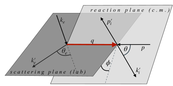
Figure 1: Kinematics of an electroproduction experiment with the final meson-baryon state $i$. The scattering plane is defined by the respective in/outgoing electron momenta $k_{e}/k_{e}^{\prime}$ with the electron scattering angle $\theta_{e}$. The reaction plane is spanned by the virtual photon and the outgoing meson, scattered by an angle $\theta$.

As discussed in the previous paper Mai et al. (2021) based on the seminal papers Chew et al. (1957); Dennery (1961); Berends et al. (1967); Ciofi Degli Atti (1978), the process of a photon-induced production of a meson off a nucleon is encoded in the transition amplitude. In the one-photon approximation, and considering the continuity equation for the current, the latter can be expressed in terms of three independent multipoles for a fixed quantum number $\ell_{\pm}$ of the final meson-baryon state. We chose those to be electric, magnetic and longitudinal multipoles $E_{\ell\pm}(W,Q^{2})$, $M_{\ell\pm}(W,Q^{2})$ and $L_{\ell\pm}(W,Q^{2})$ with the latter related to the often-used Coulomb multipole as $\omega C_{\ell\pm}(W,Q^{2})=qL_{\ell\pm}(W,Q^{2})$. Each of the introduced multipoles carry a discrete index corresponding to the total angular momentum $J=\ell\pm 1/2$ and final-state index $\mu$, e.g., $E^{\eta p}_{0+}$.

We construct the electroproduction multipoles on the basis of the dynamical coupled-channel Jülich-Bonn (JüBo) approach Rönchen et al. (2013, 2014) that provides the boundary condition at $Q^{2}=0$, incorporating the experimental information from real-photon and pion-induced reactions. In this approach, two-body unitarity and analyticity are respected and the baryon resonance spectrum is determined in terms of poles in the complex energy plane on the second Riemann sheet Döring et al. (2009a, b).

Extending the ansatz of the JüBo approach, we begin by introducting a generic function ($\bar{\cal{M}}$) for each electromagnetic multipole (${\cal M}_{\mu\gamma^{*}}\in\{E_{\mu},L_{\mu},M_{\mu}\}$) as

$$\mkern 1.5mu\overline{\mkern-1.5mu\cal M\mkern-1.5mu}\mkern 1.5mu_{\mu\gamma^{*}} (k,W,Q^{2})=V_{\mu\gamma^{*}}(k,W,Q^{2})$$ (3)

$$+ \sum_{\kappa}\int\limits_{0}^{\infty}dp\,p^{2}\,T_{\mu\kappa}(k,p,W)G_{\kappa}(p,W)V_{\kappa\gamma^{*}}(p,W,Q^{2})\,,$$

where the summation extends over intermediate meson-baryon channels $\kappa\in\{\pi N,\eta N,K\Lambda,K\Sigma,\pi\Delta,\rho N\}$. Note that the $\sigma N$ channel is not part of this list. The $\sigma N$ channel is part of the final-state interaction, but neither the hadronic resonance vertex functions nor the photon is directly coupled to it; once two-pion photon or electroproduction data are analyzed, such couplings will become relevant and will be included.

The electroproduction kernel $V_{\mu\gamma^{*}}$ in Eq. (3) is parametrized as

$$V_{\mu\gamma^{*}}(p,W,Q^{2})= \alpha^{NP}_{\mu\gamma^{*}}(p,W,Q^{2})$$ (4)

$$+\sum_{i=1}^{i_{\text{max}}}\frac{\gamma^{a}_{\mu;i}(p)\gamma^{c}_{\gamma^{*};i}(W,Q^{2})}{W-m^{b}_{i}}\,,$$

introducing the $Q^{2}$-dependence via a separable ansatz,

$$\alpha^{NP}_{\mu\gamma^{*}}(p,W,Q^{2}) ={\tilde{F}}_{\mu}(Q^{2})\alpha^{NP}_{\mu\gamma}(p,W)\,,$$

$$\gamma^{c}_{\gamma^{*};i}(W,Q^{2}) ={\tilde{F}}_{i}(Q^{2})\gamma^{c}_{\gamma;i}(W)\,.$$ (5)

The $Q^{2}$-independent pieces on the right hand side of both equations represent the input from the JüBo2017 solution Rönchen et al. (2018). Specifically, $\gamma^{c}_{\gamma;i}$ describes the interaction of the photon with the resonance state $i$ with bare mass $m_{i}^{b}$ and $\alpha^{NP}_{\mu\gamma}$ accounts for the coupling of the photon to the so-called background or non-pole part of the amplitude. Both quantities are parametrized by energy-dependent polynomials, see Ref. Rönchen et al. (2014).

The $Q^{2}$ dependence is encoded entirely in the channel-dependent form-factor ${\tilde{F}}_{\mu}(Q^{2})$ and another channel-independent form-factor ${\tilde{F}}_{i}(Q^{2})$ that depends on the resonance index $i$. We emphasize that this structure is inherited from the JüBo photoproduction ansatz, which separates the photon-induced vertex ($\gamma^{c}$) from the decay vertex of a resonance to the final meson-baryon pair ($\gamma_{\mu}^{a}$). Both ${\tilde{F}}_{\mu}(Q^{2})$ and ${\tilde{F}}_{i}(Q^{2})$ are chosen as

$${\tilde{F}}_{\mu}(Q^{2}) ={\tilde{F}}_{D}(Q^{2})\,e^{-\beta_{\mu}^{0}Q^{2}/m^{2}}\,P^{N}(Q^{2}/m^{2},\vec{\beta}_{\mu})\,,$$

$${\tilde{F}}_{i}(Q^{2}) ={\tilde{F}}_{D}(Q^{2})\,e^{-\delta_{i}^{0}Q^{2}/m^{2}}\,P^{N}(Q^{2}/m^{2},\vec{\delta}_{i})\,,$$ (6)

where $P^{N}(x,\vec{y})=1+xy_{1}+...+x^{N}y_{N}$ is a general polynomial with free parameters to be fitted together with $\delta_{i}^{0}$ and $\beta^{0}_{\mu}$ to experimental electroproduction data. The parameter-free form factor ${\tilde{F}}_{D}(Q^{2})$ encodes the empirical dipole behavior, usually implemented in such problems, as well as a Woods-Saxon form factor which ensures suppression at large $Q^{2}$. It reads

$${\tilde{F}}_{D}(Q^{2})=\frac{1}{(1+Q^{2}/b^{2})^{2}}\,\frac{1+e^{-Q_{r}^{2}/Q_{w}^{2}}}{1+e^{(Q^{2}-Q_{r}^{2})/Q_{w}^{2}}}$$ (7)

with $b^{2}=0.71$ GeV², $Q_{w}^{2}=0.5~{}{\rm GeV}^{2}$ and $Q_{r}^{2}=4.0~{}{\rm GeV}^{2}$, see Ref. Mai et al. (2021) for more details

As stated above, this procedure relies heavily on the input from the photoproduction, i.e., the functions $\alpha^{NP}_{\mu\gamma}(p,W)$ and $\gamma^{c}_{\gamma;i}(W)$. Obviously, such an input cannot exist for the longitudinal multipoles as their contribution vanishes exactly at the photon-point. In this case we employ a strategy similar to that of Ref. Mai et al. (2012):

1) We recall that at the pseudo-threshold ($q=0$) the electric and longitudinal multipoles relate according to the Siegert’s condition as

$$\frac{E_{\ell+}}{L_{\ell+}}\Big{|}_{q=0}=1\,,\qquad\frac{E_{\ell-}}{L_{\ell-}}\Big{|}_{q=0}=\frac{\ell}{1-\ell}\,.$$ (8)

For more details, see Sec. 2.2-2.3 of Ref. Mai et al. (2012), or the original derivations in Refs. Ciofi Degli Atti (1978); Tiator (2016). Therefore, we apply at the nearest pseudo-threshold point, $Q^{2}_{\rm PT}=-(W-m)^{2}$,

$$\alpha^{NP,L_{\ell\pm}}_{\mu\gamma^{*}}(p,W,Q^{2}) =\frac{\omega}{\omega_{\rm PT}}\frac{{\tilde{F}}_{D}(Q^{2})}{{\tilde{F}}_{D}(Q^{2}_{\rm PT})}$$ (9)

$$\times D_{\mu}^{\ell\pm}(W,Q^{2})\alpha^{NP,E_{\ell\pm}}_{\mu\gamma^{*}}(p,W,Q^{2}_{\rm PT})\,,$$

and

$$\gamma^{c,L_{\ell\pm}}_{\gamma^{*};i}(W,Q^{2})=\frac{\omega}{\omega_{\rm PT}} \frac{{\tilde{F}}_{D}(Q^{2})}{{\tilde{F}}_{D}(Q^{2}_{\rm PT})}$$ (10)

$$\times\tilde{D}_{i}^{\ell\pm}(W,Q^{2})\gamma^{c,E_{\ell\pm}}_{\gamma^{*};i}(W,Q^{2}_{\rm PT})\,.$$

The photon energy is $\omega_{\rm PT}=(W^{2}-m^{2}-Q_{\rm PT}^{2})/(2W)$. The new functions $D^{\ell\pm}(Q^{2})$ ensure Siegert’s condition and consistent falloff behavior in $Q^{2}$ as

$$D_{\mu}^{\ell+}(W,Q^{2}) =e^{-\beta_{\mu}^{0}q/q_{\gamma}}\,P^{N}(q/q_{\gamma},\vec{\beta}_{\mu})\,,$$ (11)

$$\tilde{D}_{i}^{\ell+}(W,Q^{2}) =e^{-\delta_{i}^{0}q/q_{\gamma}}\,P^{N}(q/q_{\gamma},\vec{\delta}_{i})\,,$$

$$D_{\mu}^{\ell-}(W,Q^{2}) =-\frac{\ell-1}{\ell}e^{-\beta_{i}^{0}q/q_{\gamma}}\,P^{N}(q/q_{\gamma},\vec{\beta}_{\mu})\,,$$

$$\tilde{D}_{i}^{\ell-}(W,Q^{2}) =-\frac{\ell-1}{\ell}e^{-\delta_{i}^{0}q/q_{\gamma}}\,P^{N}(q/q_{\gamma},\vec{\delta}_{i})\,,$$

respectively to the pole and non-pole part for $q_{\gamma}=q(Q^{2}=0)$.

2) In two specific cases ($(\ell\pm,I)=(1-,1/2)$ and $(\ell\pm,I)=(1-,3/2)$) the electric multipole vanishes due to selection rules, rendering the implementation of Siegert’s theorem nonsensical. In these cases, we obtain the longitudinal multipole from the magnetic one using a new real-valued normalization constants $\zeta^{NP}$ to be determined from the fit,

$$\alpha^{NP,L_{\ell\pm}}_{\mu\gamma^{*}}(p,W,Q^{2}) =\zeta^{NP}_{\mu}\frac{\omega}{\omega_{\rm PT}}{\tilde{F}}^{\mu}(Q^{2})$$ (12)

$$\qquad\times\alpha^{NP,M_{\ell\pm}}_{\mu\gamma^{*}}(p,W)\,,$$

$$\gamma^{c,L_{\ell\pm}}_{\gamma^{*};i}(W,Q^{2}) =\zeta_{i}\frac{\omega}{\omega_{\rm PT}}{\tilde{F}}^{\mu}(Q^{2})\gamma^{c,M_{\ell\pm}}_{\gamma;i}(W)\,.$$

Before writing down the final relation between the generic multipole functions ($\bar{E}_{\ell\pm}$, $\bar{M}_{\ell\pm}$, $\bar{L}_{\ell\pm}$) and corresponding multipoles, we note that the latter obey a certain behavior at the pseudo- ($q=0$) and production threshold ($k=0$)

$$\ell\geq 0:\quad\lim_{k\to 0}E_{\ell+}=k^{\ell}~{}, \lim_{q\to 0}E_{\ell+}=q^{\ell}~{},$$

$$\ell\geq 0:\quad\lim_{k\to 0}L_{\ell+}=k^{\ell}~{}, \lim_{q\to 0}L_{\ell+}=q^{\ell}~{},$$

$$\phantom{\ell=1:}\quad\lim_{k\to 0}L_{1-}=k~{}, \lim_{q\to 0}L_{1-}=q~{},$$

$$\ell\geq 1:\quad\lim_{k\to 0}M_{\ell\pm}=k^{\ell}~{}, \lim_{q\to 0}M_{\ell\pm}=q^{\ell}~{},$$

$$\ell\geq 2:\quad\lim_{k\to 0}E_{\ell-}=k^{\ell}~{}, \lim_{q\to 0}E_{\ell-}=q^{\ell-2}~{},$$

$$\ell\geq 2:\quad\lim_{k\to 0}L_{\ell-}=k^{\ell}~{}, \lim_{q\to 0}L_{\ell-}=q^{\ell-2}~{}.$$ (13)

We incorporate these conditions using

$${\cal M}_{\mu\gamma^{*}}(k,W,Q^{2})=R_{\ell^{\prime}}(\lambda,q/q_{\gamma})\mkern 1.5mu\overline{\mkern-1.5mu\cal M\mkern-1.5mu}\mkern 1.5mu_{\mu\gamma^{*}}(k,W,Q^{2})$$ (14)

for each multipole type and total angular momentum individually. Here,

$$R_{\ell^{\prime}}(\lambda,r) =\frac{B_{\ell^{\prime}}(\lambda r)}{B_{\ell^{\prime}}(\lambda)}$$ (15)

$$\text{with}\quad\ell^{\prime}=\left\{\begin{matrix}\ell,~{}~{}\text{for}~{}E_{\ell+},L_{\ell\pm},M_{\ell\pm}~{},~{}~{}~{}\\ \ell-2,~{}~{}\text{for}~{}E_{\ell-},L_{\ell-}\text{ and }\ell\geq 2\,,\end{matrix}\right.$$

using Blatt-Weisskopf barrier-penetration factors Blatt and Weisskopf (1952); Manley et al. (1984),

$$B_{0}(r)=1\,,$$ (16)

$$B_{1}(r)=r/\sqrt{1+r^{2}}\,,$$

$$B_{2}(r)=r^{2}/\sqrt{9+3r^{2}+r^{4}}\,,$$

$$B_{3}(r)=r^{3}/\sqrt{225+45r^{2}+6r^{4}+r^{6}}\,,$$

$$B_{4}(r)=r^{4}/\sqrt{11025+1575r^{2}+135r^{4}+10r^{6}+r^{8}}\,.$$

New free parameters $\lambda$ need to be determined from a fit to experimental data. For simplicity and to keep the number of parameters low, the $\lambda$s are chosen as channel independent.

In summary, for every partial wave, the multipoles $E_{\mu\gamma^{*}}$, $M_{\mu\gamma^{*}}$ and $L_{\mu\gamma^{*}}$ are fully determined up to: (1) $(1+N)$ channel-dependent fit parameters $\beta^{0}_{\mu},...,\beta^{N}_{\mu}$ for the non-pole part; (2) $(1+N)$ channel-independent parameters $\delta^{0}_{i},...,\delta^{N}_{i}$ for each of the $i_{\text{max}}$ resonances; (3) one channel-independent threshold behavior regulating parameter $\lambda$; (4) channel-(in)dependent normalization factors $\zeta^{NP}_{\mu}(\zeta_{i})$. Finally, any observable can be constructed from the described multipoles using a standard procedure involving CGLN and helicity amplitudes Chew et al. (1957). For explicit formulas we refer the reader to the previous publication Mai et al. (2021).

III Previous single-channel fits

Before discussing our findings for the coupled-channel case, we review what has been learned from fits to the eta electroproduction data alone. The etaMAID model Chiang et al. (2002) is similar to the MAID2007 analysis Drechsel et al. (2007) of pion production, with the fit including both eta photo- and electroproduction data. It differs from MAID2007 by a phase factor which was adjusted to the corresponding pion-nucleon phase. For eta photo- and electroproduction this was not found to be feasible, due to the quality and range of available $\eta N$ production data. As a result, there exists an overall phase ambiguity, in comparisons of different eta photoproduction fits, which cannot be determined experimentally. Comparing the eta photoproduction fits of etaMAID and the Jülich-Bonn approach, overall qualitative agreement is improved by applying a simple overall sign. This is illustrated in Fig. 2.

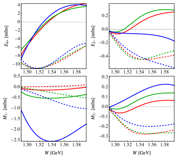
Figure 2: Selected eta photoproduction multipoles in the isospin basis from JüBo Rönchen et al. (2018) (blue), etaMAID Chiang et al. (2002) (red) and Bonn-Gatchina Anisovich et al. (2012b) (green) approaches. Real and imaginary parts are depicted by full and dashed lines, respectively. A phase factor $(-1)$ is applied to the etaMAID solution.

The overall phase, applied to etaMAID, yeilds a quantitative agreement between the JüBo, etaMAID, and Bonn-Gatchina determinations of the $E_{0+}$ multipole. The $M_{2-}$ multipole shows qualitative agreement, while the $M_{1-}$ and $E_{2-}$ multipoles show differences in sign and scale that hinder a comparison of electroproduction results extrapolated to $Q^{2}=0$.

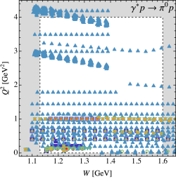
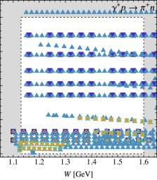
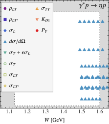
Figure 3: Experimental data Mertz et al. (2001); Elsner et al. (2006); Joo et al. (2003); Sparveris et al. (2003); Kelly et al. (2005); Bartsch et al. (2002); Bensafa et al. (2007); Laveissiere et al. (2004); Ungaro et al. (2006); Gayler (1971); May (1971); Hill (1977); Joo et al. (2002); Frolov et al. (1999); Siddle et al. (1971); Haidan (1979); Kalleicher et al. (1997); Baetzner et al. (1974); Latham et al. (1979, 1981); Stave (2006); Sparveris et al. (2007); Alder et al. (1976); Afanasev et al. (1975); Shuttleworth et al. (1972); Blume et al. (1983); Rosenberg (1979); Gerhardt (1979); Kunz et al. (2003); Stave et al. (2006); Sparveris et al. (2005); Warren et al. (1998); Pospischil et al. (2001); Joo et al. (2004); K. Park, private communication (2007); Gaskell et al. (2001); Egiyan et al. (2006); Breuker et al. (1978a); Bardin et al. (1975, 1977); Davenport (1980); Vapenikova et al. (1988); Alder et al. (1975); Evangelides et al. (1974); Breuker et al. (1982, 1983); Alder et al. (1975); Armstrong et al. (1999); Denizli et al. (2007); Thompson et al. (2001) used in the present analysis (aggregated values of $\theta,\,\phi,\,\epsilon$). The white dashed rectangles represent the considered fitting window $(0<Q^{2}/{\rm GeV}^{2}<4,1.13<W/{\rm GeV}<1.6)$.

The eta electroproduction fit of etaMAID requires a determination of the $Q^{2}$ dependence, which is chosen to be simpler than what was used for pion electroproduction (MAID2007). The dominant S-wave multipole near threshold, in principle, includes both the $N(1535)$ and $N(1650)$ resonance contributions. These have been combined using a single-quark transition model Burkert and Li (1993). For the $N(1535)$ multipole, the $Q^{2}$ dependence is assumed to be proportional to a dipole form factor multiplied by a ratio of linear functions of $Q^{2}$. Other resonance multipoles have $Q^{2}$ dependence approximated by a simple dipole factor multiplied by a ratio of kinematic factors.

Included in etaMAID are the above mentioned $N(1535)$ and $N(1650)$, together with the $N(1520)$, $N(1675)$, $N(1700)$, $N(1710)$, and $N(1720)$. Of these, the $N(1650)$, $N(1675)$, $N(1710)$, and $N(1720)$ were found to have $\eta N$ branching ratios at the 3 - 26% level; the $N(1520)$, $N(1680)$, and $N(1700)$ contributed with branching ratios less than 1%. The $N(1535)$ had a 50% branching to the $\eta N$ channel; there is universal agreement on this branching to the 10% level. Included in the fit were data available as of 2001, the cross section measurements of Ref. Armstrong et al. (1999) and Ref. Thompson et al. (2001).

The data of Ref. Armstrong et al. (1999) were taken for $Q^{2}$ values of 2.4 and 3.6 GeV², and for c.m. energies between approximately 1.5 and 1.6 GeV. Cross sections show, within uncertainties, a flat angular distribution, independent of the angle $\phi$. Based on this and a relativistic quark model expectation Ravndal (1971) that longitudinal contributions should be small, a Breit-Wigner-plus-background fit was done to extract the $N(1535)$ contribution. The authors of Ref. Ravndal (1971) concluded that the background was consistent with zero and terms beyond an S-wave approximation amounted to less than 7%. The size of longitudinal contributions had also been explored experimentally Brasse et al. (1978); Breuker et al. (1978b) by varying $\epsilon$ in order to extract the ratio of longitudinal and transverse cross sections. This ratio for $Q^{2}$ values between 0.4 and 1.0 GeV², and c.m. energies corresponding to the $N(1535)$, was found to be about 20% with 100% uncertainties. Cross sections up to a c.m. energy of 1.9 GeV, for $Q^{2}$ between 0.15 to 1.5 GeV², were measured in Ref Thompson et al. (2001). Here, the cross section was fitted to an expansion in multipoles up to $J=3/2$. Unlike Ref. Armstrong et al. (1999), evidence for significant interference between S- and P-wave contributions was found with cross sections displaying $\theta$ dependence also at a c.m. energy corresponding to the $N(1535)$.

Data from Ref. Denizli et al. (2007) have the benefit of a wide kinematic range, with c.m. energies between 1.5 and 2.3 GeV, and $Q^{2}$ values from 0.13 to 3.3 GeV². Cross sections were expanded in terms of Legendre polynomials. Here too, the angular behavior was concluded to be mainly due to interference between S- and P-wave contribution, though they could not distinguish between the $N(1710)$ and $N(1720)$ as a source. Fits to this data set tended to show more $\phi$ dependence in the cross section near the $N(1535)$ than was given in the etaMAID result – though these data were not included in the etaMAID solution.

Data from Ref. Dalton et al. (2009) covers the c.m. energy range from threshold to 1.8 GeV for $Q^{2}$ values of 5.7 and 7.0 GeV². Angular behavior is again attributed to S- and P-wave interference. There is evidence that this interference may change sign in going from lower to higher values of $Q^{2}$. EtaMAID appears to give a reasonable qualitative description of the data even at these high $Q^{2}$ values, even though these data were not included in the fit.

IV Data and fits

By design, the introduced framework is capable of addressing the electroproduction multipoles and observables simultaneously in all considered channels $\{\pi N,\eta N,K\Lambda,K\Sigma,\pi\Delta,\rho N\}$. Experimentally, the most extensively explored final-state channels are $\pi N$, $\eta N$, and $K\Lambda$. Therefore, and also extending upon the already available single channel JBW analysis of Ref. Mai et al. (2021), we first restrict the data base to pion and eta final states within the same kinematical range, i.e., $0<Q^{2}/{\rm GeV}^{2}<4$, $1.13<W/{\rm GeV}<1.6$. However, we emphasize that all two-body channels and all spin configurations of the three-body channels $\rho N$, $\pi\Delta$, and $p\sigma$ are considered in the intermediate states. The data coverage in this kinematical window is summarized in Fig. 3.

The new $\eta N$ data set consists entirely of differential cross sections, given by

$$\frac{d\sigma}{d\Omega_{e}^{\prime}dE_{\rm f}d\Omega} =\left(\frac{\alpha}{2\pi^{2}}\frac{E_{e}^{\prime}}{E_{e}}\frac{q_{L}}{Q^{2}}\frac{1}{1-\epsilon}\right)\frac{d\sigma^{v}}{d\Omega}\,,$$ (17)

where $\Omega$ refers to the angles of the final meson-baryon system ($\theta$, $\phi$) and $\Omega_{e}^{\prime}$ are the angles of the final electron at energy $E_{e}^{\prime}$. The energy of the initial electron is denoted by $E_{e}$. The differential cross section $d\sigma^{v}/d\Omega$ for the virtual photon sub-process is commonly further decomposed as

$$\frac{d\sigma^{v}}{d\Omega}= \sigma_{T}+\epsilon\sigma_{L}+\sqrt{2\epsilon(1+\epsilon)}\sigma_{LT}\cos{\phi}$$

$$+\epsilon\sigma_{TT}\cos{2\phi}+h\sqrt{2\epsilon(1-\epsilon)}\sigma_{LT^{\prime}}\sin{\phi}\,.$$ (18)

In contrast, in both $\pi N$ channels also polarization data have been measured which are connected to the multipoles as described explicitly in Ref. Mai et al. (2021). As discussed there, when both differential cross section data and structure functions ($\sigma_{T}$, $\sigma_{L}$, $\sigma_{TT}$, $\sigma_{LT}$, and $\sigma_{LT^{\prime}}$) were available from the same experiment at the same kinematics, double counting was avoided with preference given to the differential cross section data. This is statistically more sound, as correlations between separated contributions to the differential cross section data are typically not quoted.

Type	$N_{\rm data}^{\pi^{0}p}$	$N_{\rm data}^{\pi^{+}n}$	$N_{\rm data}^{\eta p}$
$\rho_{LT}$	45 Mertz et al. (2001); Elsner et al. (2006)	–	–
$\rho_{LT^{\prime}}$	2644 Joo et al. (2003); Sparveris et al. (2003); Kelly et al. (2005); Bartsch et al. (2002); Bensafa et al. (2007)	4354 Joo et al. (2004); K. Park, private communication (2007)	–
$\sigma_{L}$	–	2 Gaskell et al. (2001)	–
$d\sigma/d\Omega$	39942 Laveissiere et al. (2004); Ungaro et al. (2006); Gayler (1971); May (1971); Hill (1977); Joo et al. (2002); Frolov et al. (1999); Siddle et al. (1971); Haidan (1979); Sparveris et al. (2003); Kelly et al. (2005); Kalleicher et al. (1997); Baetzner et al. (1974); Latham et al. (1979, 1981); Stave (2006); Sparveris et al. (2007); Alder et al. (1976); Afanasev et al. (1975); Shuttleworth et al. (1972); Blume et al. (1983); Rosenberg (1979); Gerhardt (1979)	32813 Egiyan et al. (2006); Breuker et al. (1978a); K. Park, private communication (2007); Bardin et al. (1975, 1977); Gerhardt (1979); Davenport (1980); Vapenikova et al. (1988); Hill (1977); Alder et al. (1975); Evangelides et al. (1974); Breuker et al. (1982, 1983)	1874 Armstrong et al. (1999); Denizli et al. (2007); Thompson et al. (2001)
$\sigma_{T}+\epsilon\sigma_{L}$	318 Laveissiere et al. (2004); Mertz et al. (2001); Sparveris et al. (2003); Kunz et al. (2003); Stave et al. (2006); Sparveris et al. (2007, 2005); Alder et al. (1976)	144 Breuker et al. (1978a); Alder et al. (1975)	–
$\sigma_{T}$	10 Blume et al. (1983)	2 Gaskell et al. (2001)	–
$\sigma_{LT}$	312 Laveissiere et al. (2004); Sparveris et al. (2003); Mertz et al. (2001); Kunz et al. (2003); Stave et al. (2006); Sparveris et al. (2007, 2005); Alder et al. (1976)	106 Breuker et al. (1978a); Alder et al. (1975)	–
$\sigma_{LT^{\prime}}$	198 Joo et al. (2003); Kunz et al. (2003); Stave et al. (2006); Sparveris et al. (2007)	192 Joo et al. (2003)	–
$\sigma_{TT}$	266 Laveissiere et al. (2004); Stave et al. (2006); Sparveris et al. (2007, 2005); Alder et al. (1976)	91 Breuker et al. (1978a); Alder et al. (1975)	–
$K_{D1}$	1527 Kelly et al. (2005)	–	–
$P_{Y}$	–	2 Warren et al. (1998); Pospischil et al. (2001)	–

Table 1: Data used in the fit, separated by observable type and final state.

To study constraints of the experimental data on the present coupled-channel formalism, we employ the following fit strategies. First, starting with the fit results of the pion-electroproduction analysis Mai et al. (2021), including S-, P- and D-waves, while setting $N=2$ in Eq. (6), we allow for 40 new parameters,

$$\beta^{0}_{\eta N}\,,~{}\beta^{1}_{\eta N}\,,~{}\beta^{2}_{\eta N}~{}, \quad\text{for}\quad E_{\ell\pm},L_{\ell\pm},M_{\ell\pm}\text{~{}and~{}}\ell\leq 2\,,$$

$$\zeta^{NP}_{\eta N}~{}, \quad\text{for}\quad L_{1-}~{},$$ (19)

in addition to the 209 previously Mai et al. (2021) available parameters. Specifically, for all intermediate channels we chose again $\zeta^{NP}_{\mu\neq\eta N}\equiv\zeta^{NP}_{\pi N}$ and $\beta_{\mu\notin\{\pi N,\eta N\}}^{i\in\{0,1,2\}}=0$. Second, starting from any of the four best fit results of Ref. Mai et al. (2021) and holding all but the new parameters fixed, we minimize a regular $\chi^{2}$ function

$$\chi^{2}_{\rm reg}=\sum_{i=1}^{N_{\rm all}}\left(\frac{\mathcal{O}_{i}^{\rm exp}-\mathcal{O}_{i}}{\Delta_{i}^{\rm stat}+\Delta^{\rm syst}_{i}}\right)^{2}\,,$$ (20)

with respect to the $\pi^{0}p,\pi^{+}n,\eta p$ channels simultaneously. The data, as taken from SAID, contain also systematic uncertainties $\Delta^{\rm syst}$ that are separately quoted in the data base GWU, SAID website (2021). We note that the database sizes are vastly different in these channels. Thus, this simple choice of the $\chi^{2}$ function might marginalize the influence of the smaller $\eta N$ dataset. To test this hypothesis, we additionally perform a minimization with respect to a commonly used weighting scheme (for a typical application see, e.g.,  Mai and Meißner (2013)),

$$\chi^{2}_{\rm wt}=\sum_{j\in\{\pi^{0}p,\pi^{+}n,\eta p\}}\frac{N_{\rm all}}{3N_{j}}\sum_{i=1}^{N_{j}}\left(\frac{\mathcal{O}_{ji}^{\rm exp}-\mathcal{O}_{ji}}{\Delta_{ji}^{\rm stat}+\Delta^{\rm syst}_{ji}}\right)^{2}\,.$$ (21)

Third, after the minimization routine (utilizing MINUIT library James (1994)) has converged, all $209+40=249$ parameters are relaxed and the minimization is repeated leading to the eight different solutions $\{\mathfrak{F}^{\rm reg}_{1},...,\mathfrak{F}^{\rm reg}_{4},\mathfrak{F}^{\rm wt}_{1},...,\mathfrak{F}^{\rm wt}_{4}\}$, discussed in the next section.

V Results

	$\chi^{2}/{\rm dof}$	$\chi^{2}_{\pi^{0}p/\rm data}$	$\chi^{2}_{\pi^{+}n/\rm data}$	$\chi^{2}_{\eta p/\rm data}$
$\mathfrak{F}^{\rm reg}_{1}$	1.66	1.68	1.61	1.77
$\mathfrak{F}^{\rm reg}_{1}$	1.73	1.71	1.71	2.29
$\mathfrak{F}^{\rm reg}_{1}$	1.69	1.69	1.66	1.89
$\mathfrak{F}^{\rm reg}_{1}$	1.69	1.7	1.64	2.05
$\mathfrak{F}^{\rm wt}_{1}$	1.54	1.74	1.63	1.25
$\mathfrak{F}^{\rm wt}_{1}$	1.63	1.82	1.79	1.27
$\mathfrak{F}^{\rm wt}_{1}$	1.58	1.74	1.73	1.27
$\mathfrak{F}^{\rm wt}_{1}$	1.58	1.79	1.6	1.33

Table 2: Fit results of the coupled-channel JBW analysis with respect to $\pi N$ and $\eta N$ data. The second column shows results of a fit using standard (20) (’reg’) and weighted (21) (’wt’) $\chi^{2}$ functions, respectively, whereas the last three columns separate out contributions for individual final-state channels (per datum).

Each of the followed fit strategies led to a successful description of both considered channels. The fit results are collected in Table 2 including contributions separated out for each of the considered final-state channels ($\pi^{0}p$, $\pi^{+}n$, $\eta p$). As expected, fit results relying on the weighted version of the $\chi^{2}$ function (21) led to a much better description of the $\eta p$ data, which are much sparser than the $\pi N$ data. When comparing the individual contributions to those of the previous JBW single-channel study Mai et al. (2021) we note that the description of both $\pi N$ channels is similar in the present coupled-channel analysis. The same holds true for the contributions to subsets of data separated with respect to individual observable types. For more details on the $\pi N$ channels, see Ref. Mai et al. (2021) as well as the interactive JBW homepage JBW Interactive Scattering Analysis website (2021) (under development).

Taking a closer look on the fit results we find a relatively weak $\phi$-dependence in the data and corresponding fits, see Figs. 4 and 5. In the latter figure, there are two data points from Ref. Thompson (2000) for each angle $\theta$ at a fixed value of $\phi$. These were obtained from measurements at azimuthal angles $\phi$ and $(360-\phi)$, respectively. The cross sections were averaged in Ref. Thompson et al. (2001), but both values are retained in our database. In Fig. 6 we compare fits and data at nearby kinematic points for which the fit curves are nearly identical. This gives a visual comparison of the data consistency.

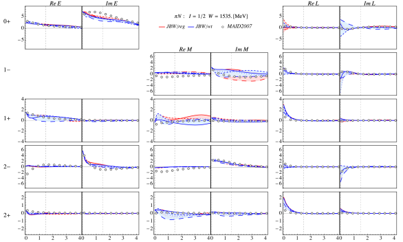
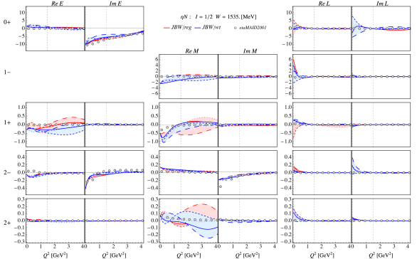
Figure 8: JBW coupled-channel results. Multipoles (in mfm) in the $\pi N$ and $\eta N$ $I=1/2$ channel at $W=1535~{}{\rm MeV}$ in comparison to the result of the MAID2007 Drechsel et al. (2007) and etaMAID2001 Chiang et al. (2002) analyses, respectively. The latter results are extracted from the MAID homepage and multiplied by $-1/\sqrt{3}$, adjusting for a phase- and isospin factor. The leftmost column shows the total angular momentum. Fits correspond to the results of Tab. 2 with the same line shape coding as in Ref Mai et al. (2021).

As for underlying multipoles, we found that in most cases longitudinal multipoles are subdominant to electric and magnetic ones. An overview of all considered multipoles is shown in Fig. 8 for the c.m. energy fixed to 1535 MeV. There, in most cases and within the systematic uncertainties of our approach — quantified by the spread of predictions from fits $\{\mathfrak{F}^{\rm reg}_{1},...,\mathfrak{F}^{\rm reg}_{4},\mathfrak{F}^{\rm wt}_{1},...,\mathfrak{F}^{\rm wt}_{4}\}$ — we observe an agreement with the MAID2007 ($\pi N$) and etaMAID ($\eta N$) multipole predictions. The isospin $I=1/2$ $\pi N$ multipoles are shown in the same figure with the pertinent comparison to the MAID2007 solution for convenience.

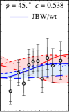
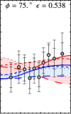
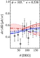
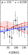
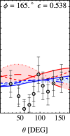
Figure 4: Selected subset of $\eta N$ data for $W=1.5~{}{\rm GeV}$, $Q^{2}=1.2~{}{\rm GeV}^{2}$ from Ref. Denizli et al. (2007). The four red and blue lines, respectively, correspond to the “reg” and “wt” solutions of Table 2.

Fixing the virtuality $Q^{2}$ to some values of interest the multipoles are shown in Figs. 9 and 10. There, we observe that the dominant $E_{0+}$ multipole agrees well with that of the etaMAID parametrization when correcting for the phase convention ($-1$) and isospin factor ($1/\sqrt{3}$). To be clear, we show our multipoles in the isospin basis, which make them smaller by a factor of $1/\sqrt{3}$ compared to the etaMAID multipoles which are quoted in the particle basis. As the results show, longitudinal multipoles seem indeed very small compared to the electric and magnetic ones. Interestingly, the $M_{2-}$ multipole seems to have a similar trend as that of the MAID solution, while the corresponding uncertainties seem to change with different $Q^{2}$ values. This can be attributed to the gaps in $\eta p$ data at some fixed $Q^{2}$ kinematics, see next section.

Finally, we demonstrate in Fig. 7 the full $Q^{2}$ vs $W$ dependence of the $E_{0+}$ and $M_{2-}$ multipoles, corresponding to quantum numbers of the $N(1535)1/2^{-}$ and $N(1520)3/2^{-}$. We observe that the systematic uncertainties discussed above are well under control. In particular, all fit solutions show a non-trivial $Q^{2}$ dependence. This supports our expectation that the helicity couplings will carry new physical information, when full $(W,Q^{2})$ information is extracted, being part of our future plans.

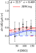
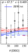
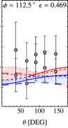
Figure 5: Selected subset of $\eta N$ data for $W=1.5~{}{\rm GeV}$, $Q^{2}=1.25~{}{\rm GeV}^{2}$ from Ref. Thompson et al. (2001); Thompson (2000). The four red and blue lines, respectively, correspond to the “reg” and “wt” solutions of Table 2.

VI Discussion and Conclusion

We have generalized our recent analysis of pion electroproduction Mai et al. (2021) to include eta electroproduction data. This allowed a coupled-channel fit up to $W=$1.6 GeV for $Q^{2}<4$ GeV². For both reactions, partial waves up to $\ell=2$ were included. Given that the pion and eta electroproduction databases are very different in size, we compared $\chi^{2}$ minimization without and with weighting factors to increase the influence of the smaller eta electroproduction dataset.

As in Ref. Mai et al. (2012), using different fit strategies, we found several solutions with nearly equivalent $\chi^{2}$/data values. The fits achieved $\chi^{2}$/data values near 1.7, similar to our previous fits to pion data alone. The fit to pion data and the resulting multipoles showed little change from the single-channel case. This result held in both weighted and unweighted fits.

Also, as in our pion electroproduction fits, the spread of results for multipoles provided a measure of systematic errors. As expected, the $E_{0+}$ multipole was reliably determined with a $Q^{2}$ dependence similar to that exhibited in etaMAID (once a phase ambiguity was accounted for).

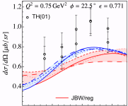
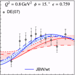
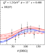
Figure 6: Selected subset of $\eta N$ data for $W=1.56~{}{\rm GeV}$ from Refs. TH(01) Thompson et al. (2001); Thompson (2000) and DE(07) Denizli et al. (2007) for similar kinematics. Result of the JBW coupled-channel fits are shown by red and blue lines corresponding to the eight best fit solutions.

The evidence for contributions from higher partial waves depends on the experiment. As mentioned, the data of Ref. Armstrong et al. (1999) are compatible with a Breit-Wigner contribution from the $N(1535)$, without any need for a background term, higher partial waves, or longitudinal multipoles, for a fit covering the energy range considered in the present analysis. The later experiment of Ref. Denizli et al. (2007), however, displays a clear forward-backward asymmetry (a sign of P-wave interference) and some evidence for D-wave interference producing a convex shape.

In our multipole solutions, there is evidence for sizeable P-wave contributions, but the spread implies the P-wave multipoles are not well determined. This is expected since the corresponding candidate states $N(1710)1/2^{+}$ and $N(1720)3/2^{+}$ are beyond the upper energy limit. Interestingly, the $M_{2-}$ multipoles are quite consistent, and appear to give a consistent value for this multipole, which also agrees with the etaMAID values away from the $Q^{2}=0$ photon point and the upper $Q^{2}$ limit of our fits.

We can understand the consistency of multipole determinations in Figs. 9 and 10, plotting multipoles versus center-of-mass energy for fixed $Q^{2}$ (0.2, 1, 2, and 3 GeV²), based on the data fitted and the constraint at $Q^{2}=0$. The lowest-$Q^{2}$ plot displays multipoles for a $Q^{2}$ value below the lower limit (0.3 GeV²) of fitted data and is close to the photoproduction point, where it was shown that the etaMAID and JüBo fits can be quite different. The behavior at $Q^{2}=3$ GeV² is supported by data from Ref. Armstrong et al. (1999) (2.4 and 3.6 GeV²) which can be fitted with only a Breit-Wigner contribution to $E_{0+}$ and shows no evidence for P- and D-waves.

The plots for intermediate $Q^{2}$ are supported by data from Refs. Thompson et al. (2001); Denizli et al. (2007), of which Ref. Denizli et al. (2007) is more precise. These plots show the most consistency for multipoles that can be determined over this narrow energy range. Note also that longitudinal multipoles are small (consistently among all our solutions) whereas this feature was built in in some earlier fits Armstrong et al. (1999).

In summary, this first coupled-channel fit to both pion and eta electroproduction data supports an expanded study. As a first step, the number of included partial-waves and the energy limits will be increased. Once completed, we will attempt an expansion to kaon electroproduction Carman et al. (2003); Ambrozewicz et al. (2007); Nasseripour et al. (2008); Carman et al. (2009, 2013); Gabrielyan et al. (2014); Achenbach et al. (2017), in the near-threshold region. We will also be in a position to explore resonance behavior at the pole as a function of $Q^{2}$ using tools developed to study the JüBo photoproduction amplitudes.

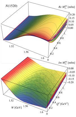
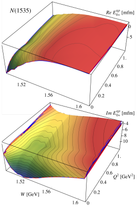
Figure 7: Predictions of $E_{0+}(W,Q^{2})$ corresponding to the quantum numbers of $N(1535)$. Different surfaces correspond to the best fit solutions obtained minimizing the regular (red boundary lines) and weighted (blue boundary lines) version of the $\chi^{2}$ function.

Acknowledgements

This work is supported by the U.S. Department of Energy, DOE Office of Science, Office of Nuclear Physics awards DE-SC0016582 and DE-SC0016583 and contract DE-AC05-06OR23177. It is also supported by the NSFC and the Deutsche Forschungsgemeinschaft (DFG, German Research Foundation) through the funds provided to the Sino-German Collaborative Research Center TRR110 “Symmetries and the Emergence of Structure in QCD” (NSFC Grant No. 12070131001, DFG Project-ID 196253076-TRR 110), by the Chinese Academy of Sciences (CAS) through a President’s International Fellowship Initiative (PIFI) (Grant No. 2018DM0034), by the VolkswagenStiftung (Grant No. 93562), and by the EU Horizon 2020 research and innovation programme, STRONG-2020 project under grant agreement No. 824093. The multipole calculation and parameter optimization are performed on the Colonial One computer cluster GWU, Colonial One High Performance Computing (2021). The authors gratefully acknowledge the computing time granted through JARA on the supercomputer JURECA Jülich Supercomputing Centre (2018) at Forschungszentrum Jülich that was used to produce the input at the photon point.

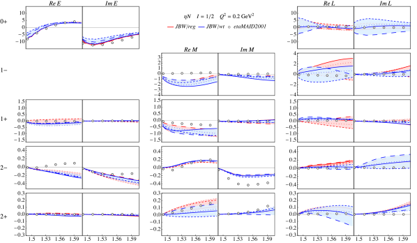
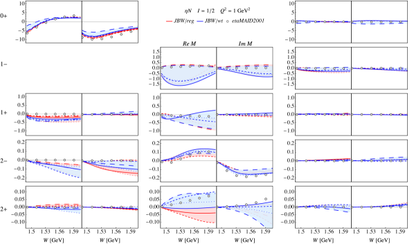
Figure 9: Eta electroproduction multipoles for lower fixed values of $Q^{2}$. Notation as given in Figure 8.

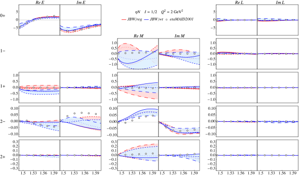
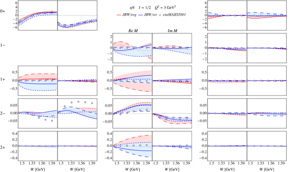
Figure 10: Eta electroproduction multipoles for higher fixed values of $Q^{2}$. Notation as given in Figure 8.

References

- Höhler (1983) G. Höhler, Methods and Results of Phenomenological Analyses / Methoden und Ergebnisse phänomenologischer Analysen, edited by H. Schopper, Landolt-Boernstein - Group I Elementary Particles, Nuclei and Atoms, Vol. 9b2 (Springer, 1983).
- Cutkosky et al. (1979) R. E. Cutkosky, R. E. Hendrick, J. W. Alcock, Y. A. Chao, R. G. Lipes, J. C. Sandusky, and R. L. Kelly, “PION - NUCLEON PARTIAL WAVE ANALYSIS,” Phys. Rev. D 20, 2804 (1979).
- Arndt et al. (2006) R. A. Arndt, W. J. Briscoe, I. I. Strakovsky, and R. L. Workman, “Extended partial-wave analysis of piN scattering data,” Phys. Rev. C 74, 045205 (2006), arXiv:nucl-th/0605082 .
- Arndt et al. (2009) R. A. Arndt, W. J. Briscoe, M. W. Paris, I. I. Strakovsky, and R. L. Workman, “Baryon Resonance Analysis from SAID,” Chin. Phys. C 33, 1063–1068 (2009), arXiv:0906.3709 [nucl-th] .
- Shrestha and Manley (2012) M. Shrestha and D. M. Manley, “Multichannel parametrization of scattering amplitudes and extraction of resonance parameters,” Phys. Rev. C 86, 055203 (2012), arXiv:1208.2710 [hep-ph] .
- Ireland et al. (2020) David G. Ireland, Eugene Pasyuk, and Igor Strakovsky, “Photoproduction Reactions and Non-Strange Baryon Spectroscopy,” Prog. Part. Nucl. Phys. 111, 103752 (2020), arXiv:1906.04228 [nucl-ex] .
- Aznauryan et al. (2009) I. G. Aznauryan et al. (CLAS), “Electroexcitation of nucleon resonances from CLAS data on single pion electroproduction,” Phys. Rev. C 80, 055203 (2009), arXiv:0909.2349 [nucl-ex] .
- Achenbach et al. (2017) P. Achenbach et al. (A1), “Beam helicity asymmetries in electroproduction off the proton at low Q2,” Eur. Phys. J. A 53, 198 (2017).
- Carman et al. (2020) D. S. Carman, K. Joo, and V. I. Mokeev, “Strong QCD Insights from Excited Nucleon Structure Studies with CLAS and CLAS12,” Few Body Syst. 61, 29 (2020), arXiv:2006.15566 [nucl-ex] .
- Beck and Thoma (2017) Reinhard Beck and Ulrike Thoma, “Spectroscopy of baryon resonances,” EPJ Web Conf. 134, 02001 (2017).
- Shiu et al. (2018) S. H. Shiu et al. (LEPS), “Photoproduction of and hyperons off protons with linearly polarized photons at GeV,” Phys. Rev. C 97, 015208 (2018), arXiv:1711.04996 [nucl-ex] .
- Akondi et al. (2019) C. S. Akondi et al. (A2), “Experimental study of the , , and reactions at the Mainz Microtron,” Eur. Phys. J. A 55, 202 (2019), arXiv:1811.05547 [nucl-ex] .
- Ho et al. (2018) D. H. Ho et al. (CLAS), “Beam-target helicity asymmetry in and photoproduction on the neutron,” Phys. Rev. C 98, 045205 (2018), arXiv:1805.04561 [nucl-ex] .
- Ohnishi et al. (2020) Hiroaki Ohnishi, Fuminori Sakuma, and Toshiyuki Takahashi, “Hadron Physics at J-PARC,” Prog. Part. Nucl. Phys. 113, 103773 (2020), arXiv:1912.02380 [nucl-ex] .
- Alef et al. (2020) S. Alef et al. (BGO-OD), “The BGOOD experimental setup at ELSA,” Eur. Phys. J. A 56, 104 (2020), arXiv:1910.11939 [physics.ins-det] .
- Zachariou et al. (2021) N. Zachariou et al. (CLAS), “Double polarisation observable for single pion photoproduction from the proton,” Phys. Lett. B 817, 136304 (2021).
- Shrestha et al. (2021) U. Shrestha et al. (CLAS), “Differential cross sections for using photoproduction at CLAS,” Phys. Rev. C 103, 025206 (2021), arXiv:2101.06134 [hep-ex] .
- Markov et al. (2020) N. Markov et al. (CLAS), “Exclusive electroproduction off protons in the resonance region at photon virtualities 0.4 GeV2 GeV2,” Phys. Rev. C 101, 015208 (2020), arXiv:1907.11974 [nucl-ex] .
- Bernard et al. (1992) Veronique Bernard, Norbert Kaiser, and Ulf G. Meißner, “On the low-energy theorems for threshold pion electroproduction,” Phys. Lett. B 282, 448–452 (1992).
- Bernard et al. (1993) Veronique Bernard, Norbert Kaiser, T. S. H. Lee, and Ulf G. Meißner, “Chiral symmetry and threshold pi0 electroproduction,” Phys. Rev. Lett. 70, 387–390 (1993).
- Bernard et al. (1994) V. Bernard, Norbert Kaiser, T. S. H. Lee, and Ulf-G. Meißner, “Threshold pion electroproduction in chiral perturbation theory,” Phys. Rept. 246, 315–363 (1994), arXiv:hep-ph/9310329 .
- Bernard et al. (1996) V. Bernard, Norbert Kaiser, and Ulf-G. Meißner, “Threshold neutral pion electroproduction in heavy baryon chiral perturbation theory,” Nucl. Phys. A 607, 379–401 (1996), [Erratum: Nucl.Phys.A 633, 695–697 (1998)], arXiv:hep-ph/9601267 .
- Hilt et al. (2013) M. Hilt, B. C. Lehnhart, S. Scherer, and L. Tiator, “Pion photo- and electroproduction in relativistic baryon chiral perturbation theory and the chiral MAID interface,” Phys. Rev. C 88, 055207 (2013), arXiv:1309.3385 [nucl-th] .
- Mai (2021) Maxim Mai, “Review of the (1405) A curious case of a strangeness resonance,” Eur. Phys. J. ST 230, 1593–1607 (2021), arXiv:2010.00056 [nucl-th] .
- Ruić et al. (2011) Dino Ruić, Maxim Mai, and Ulf-G. Meißner, “-Photoproduction in a gauge-invariant chiral unitary framework,” Phys. Lett. B 704, 659–662 (2011), arXiv:1108.4825 [nucl-th] .
- Mai et al. (2012) Maxim Mai, Peter C. Bruns, and Ulf-G. Meißner, “Pion photoproduction off the proton in a gauge-invariant chiral unitary framework,” Phys. Rev. D 86, 094033 (2012), arXiv:1207.4923 [nucl-th] .
- Bruns (2020) Peter C. Bruns, “A formalism for the study of photoproduction in the region,” (2020), arXiv:2012.11298 [nucl-th] .
- Döring and Nakayama (2010a) M. Döring and K. Nakayama, “On the cross section ratio sigma(n)/sigma(p) in eta photoproduction,” Phys. Lett. B 683, 145–149 (2010a), arXiv:0909.3538 [nucl-th] .
- Döring and Nakayama (2010b) M. Döring and K. Nakayama, “The Phase and pole structure of the N*(1535) in pi N — pi N and gamma N — pi N,” Eur. Phys. J. A 43, 83–105 (2010b), arXiv:0906.2949 [nucl-th] .
- Borasoy et al. (2007) B. Borasoy, P. C. Bruns, Ulf-G. Meißner, and R. Nissler, “A Gauge invariant chiral unitary framework for kaon photo- and electroproduction on the proton,” Eur. Phys. J. A 34, 161–183 (2007), arXiv:0709.3181 [nucl-th] .
- Meißner and Oller (2000) Ulf-G. Meißner and J. A. Oller, “Chiral unitary meson baryon dynamics in the presence of resonances: Elastic pion nucleon scattering,” Nucl. Phys. A 673, 311–334 (2000), arXiv:nucl-th/9912026 .
- Haberzettl (2021) Helmut Haberzettl, “Gauge invariance of meson photo- and electroproduction currents revisited,” Phys. Rev. D 104, 056001 (2021), arXiv:2105.11554 [hep-ph] .
- Chiang et al. (2002) Wen-Tai Chiang, Shin-Nan Yang, Lothar Tiator, and Dieter Drechsel, “An Isobar model for eta photoproduction and electroproduction on the nucleon,” Nucl. Phys. A 700, 429–453 (2002), arXiv:nucl-th/0110034 .
- Aznauryan (2003) I. G. Aznauryan, “Multipole amplitudes of pion photoproduction on nucleons up to 2-Gev within dispersion relations and unitary isobar model,” Phys. Rev. C 67, 015209 (2003), arXiv:nucl-th/0206033 .
- Drechsel et al. (2007) D. Drechsel, S. S. Kamalov, and L. Tiator, “Unitary Isobar Model - MAID2007,” Eur. Phys. J. A 34, 69–97 (2007), arXiv:0710.0306 [nucl-th] .
- Tiator et al. (2018) L. Tiator, M. Gorchtein, V. L. Kashevarov, K. Nikonov, M. Ostrick, M. Hadžimehmedović, R. Omerović, H. Osmanović, J. Stahov, and A. Švarc, “Eta and Etaprime Photoproduction on the Nucleon with the Isobar Model EtaMAID2018,” Eur. Phys. J. A 54, 210 (2018), arXiv:1807.04525 [nucl-th] .
- Hanstein et al. (1998) O. Hanstein, D. Drechsel, and L. Tiator, “Multipole analysis of pion photoproduction based on fixed t dispersion relations and unitarity,” Nucl. Phys. A 632, 561–606 (1998), arXiv:nucl-th/9709067 .
- Workman et al. (2012) Ron L. Workman, Mark W. Paris, William J. Briscoe, and Igor I. Strakovsky, “Unified Chew-Mandelstam SAID analysis of pion photoproduction data,” Phys. Rev. C 86, 015202 (2012), arXiv:1202.0845 [hep-ph] .
- Briscoe et al. (2015) William J. Briscoe, Michael Döring, Helmut Haberzettl, D. Mark Manley, Megumi Naruki, Igor I. Strakovsky, and Eric S. Swanson, “Physics opportunities with meson beams,” Eur. Phys. J. A 51, 129 (2015), arXiv:1503.07763 [hep-ph] .
- Shklyar et al. (2007) V. Shklyar, H. Lenske, and U. Mosel, “eta-photoproduction in the resonance energy region,” Phys. Lett. B 650, 172–178 (2007), arXiv:nucl-th/0611036 .
- Anisovich et al. (2012a) A. V. Anisovich, R. Beck, E. Klempt, V. A. Nikonov, A. V. Sarantsev, and U. Thoma, “Properties of baryon resonances from a multichannel partial wave analysis,” Eur. Phys. J. A 48, 15 (2012a), arXiv:1112.4937 [hep-ph] .
- Kamano et al. (2013) H. Kamano, S. X. Nakamura, T. S. H. Lee, and T. Sato, “Nucleon resonances within a dynamical coupled-channels model of and reactions,” Phys. Rev. C 88, 035209 (2013), arXiv:1305.4351 [nucl-th] .
- Rönchen et al. (2015) D. Rönchen, M. Döring, H. Haberzettl, J. Haidenbauer, U. G. Meißner, and K. Nakayama, “Eta photoproduction in a combined analysis of pion- and photon-induced reactions,” Eur. Phys. J. A 51, 70 (2015), arXiv:1504.01643 [nucl-th] .
- Nys et al. (2017) J. Nys, V. Mathieu, C. Fernández-Ramírez, A. N. Hiller Blin, A. Jackura, M. Mikhasenko, A. Pilloni, A. P. Szczepaniak, G. Fox, and J. Ryckebusch (JPAC), “Finite-energy sum rules in eta photoproduction off a nucleon,” Phys. Rev. D 95, 034014 (2017), arXiv:1611.04658 [hep-ph] .
- Mai et al. (2021) Maxim Mai, Michael Döring, Carlos Granados, Helmut Haberzettl, Ulf-G. Meißner, Deborah Rönchen, Igor Strakovsky, and Ron Workman (Jülich-Bonn-Washington), “Jülich-Bonn-Washington model for pion electroproduction multipoles,” Phys. Rev. C 103, 065204 (2021), arXiv:2104.07312 [nucl-th] .
- Rönchen et al. (2018) D. Rönchen, M. Döring, and U.-G. Meißner, “The impact of photoproduction on the resonance spectrum,” Eur. Phys. J. A 54, 110 (2018), arXiv:1801.10458 [nucl-th] .
- Kamano et al. (2016) H. Kamano, S. X. Nakamura, T. S. H. Lee, and T. Sato, “Isospin decomposition of transitions within a dynamical coupled-channels model,” Phys. Rev. C 94, 015201 (2016), arXiv:1605.00363 [nucl-th] .
- Rönchen et al. (2014) D. Rönchen, M. Döring, F. Huang, H. Haberzettl, J. Haidenbauer, C. Hanhart, S. Krewald, U.-G. Meißner, and K. Nakayama, “Photocouplings at the Pole from Pion Photoproduction,” Eur. Phys. J. A 50, 101 (2014), [Erratum: Eur.Phys.J.A 51, 63 (2015)], arXiv:1401.0634 [nucl-th] .
- Kamano et al. (2010) H. Kamano, S. X. Nakamura, T. S. H. Lee, and T. Sato, “Extraction of P11 resonances from pi N data,” Phys. Rev. C 81, 065207 (2010), arXiv:1001.5083 [nucl-th] .
- Tiator et al. (2010) L. Tiator, S. S. Kamalov, S. Ceci, G. Y. Chen, D. Drechsel, A. Svarc, and S. N. Yang, “Singularity structure of the scattering amplitude in a meson-exchange model up to energies GeV,” Phys. Rev. C 82, 055203 (2010), arXiv:1007.2126 [nucl-th] .
- Zyla et al. (2020) P. A. Zyla et al. (Particle Data Group), “Review of Particle Physics,” PTEP 2020, 083C01 (2020).
- Crede et al. (2011) V. Crede et al. (CBELSA/TAPS), “Photoproduction of Neutral Pions off Protons,” Phys. Rev. C 84, 055203 (2011), arXiv:1107.2151 [nucl-ex] .
- Anisovich et al. (2017) A. V. Anisovich, V. Burkert, J. Hartmann, E. Klempt, V. A. Nikonov, E. Pasyuk, A. V. Sarantsev, S. Strauch, and U. Thoma, “Evidence for from photoproduction and consequence for chiral-symmetry restoration at high mass,” Phys. Lett. B 766, 357–361 (2017), arXiv:1503.05774 [nucl-ex] .
- Landay et al. (2019) J. Landay, M. Mai, M. Döring, H. Haberzettl, and K. Nakayama, “Towards the Minimal Spectrum of Excited Baryons,” Phys. Rev. D 99, 016001 (2019), arXiv:1810.00075 [nucl-th] .
- Landay et al. (2017) J. Landay, M. Döring, C. Fernández-Ramírez, B. Hu, and R. Molina, “Model Selection for Pion Photoproduction,” Phys. Rev. C 95, 015203 (2017), arXiv:1610.07547 [nucl-th] .
- Drechsel et al. (1999) D. Drechsel, O. Hanstein, S. S. Kamalov, and L. Tiator, “A Unitary isobar model for pion photoproduction and electroproduction on the proton up to 1-GeV,” Nucl. Phys. A 645, 145–174 (1999), arXiv:nucl-th/9807001 .
- Arndt et al. (2002) R. A. Arndt, I. I. Strakovsky, and R. L. Workman, “Analysis of pion electroproduction data,” PiN Newslett. 16, 150–153 (2002), arXiv:nucl-th/0110001 .
- Tiator et al. (2003) L. Tiator, D. Drechsel, S. S. Kamalov, and S. N. Yang, “Electromagnetic form-factors of the Delta(1232) excitation,” Eur. Phys. J. A 17, 357–363 (2003).
- Tiator et al. (2004) L. Tiator, D. Drechsel, S. Kamalov, M. M. Giannini, E. Santopinto, and A. Vassallo, “Electroproduction of nucleon resonances,” Eur. Phys. J. A 19, 55–60 (2004), arXiv:nucl-th/0310041 .
- Aznauryan et al. (2005a) I. G. Aznauryan, V. D. Burkert, H. Egiyan, K. Joo, R. Minehart, and L. C. Smith, “Electroexcitation of the P(33)(1232), P(11)(1440), D(13)(1520), S(11)(1535) at Q**2 = 0.4 and 0.65 (GeV/c)**2,” Phys. Rev. C 71, 015201 (2005a), arXiv:nucl-th/0407021 .
- Aznauryan et al. (2005b) I. G. Aznauryan, V. D. Burkert, G. V. Fedotov, B. S. Ishkhanov, and V. I. Mokeev, “Electroexcitation of nucleon resonances at Q**2 = 0.65- (GeV/c)**2 from a combined analysis of single- and double-pion electroproduction data,” Phys. Rev. C 72, 045201 (2005b), arXiv:hep-ph/0508057 .
- Corthals et al. (2007) T. Corthals, T. Van Cauteren, P. Van Craeyveld, J. Ryckebusch, and D. G. Ireland, “Electroproduction of kaons from the proton in a Regge-plus-resonance approach,” Phys. Lett. B 656, 186–192 (2007), arXiv:0704.3691 [nucl-th] .
- Aznauryan and Burkert (2012a) I. G. Aznauryan and V. D. Burkert, “Electroexcitation of nucleon resonances,” Prog. Part. Nucl. Phys. 67, 1–54 (2012a), arXiv:1109.1720 [hep-ph] .
- Tiator et al. (2011) L. Tiator, D. Drechsel, S. S. Kamalov, and M. Vanderhaeghen, “Electromagnetic Excitation of Nucleon Resonances,” Eur. Phys. J. ST 198, 141–170 (2011), arXiv:1109.6745 [nucl-th] .
- Aznauryan et al. (2013) I. G. Aznauryan et al., “Studies of Nucleon Resonance Structure in Exclusive Meson Electroproduction,” Int. J. Mod. Phys. E 22, 1330015 (2013), arXiv:1212.4891 [nucl-th] .
- Vrancx et al. (2014) Tom Vrancx, Jan Ryckebusch, and Jannes Nys, “ electroproduction above the resonance region,” Phys. Rev. C 89, 065202 (2014), arXiv:1404.4156 [nucl-th] .
- Maxwell (2014) Oren V. Maxwell, “Recoil polarization observables in the electroproduction of K mesons and ’s from the proton,” Phys. Rev. C 90, 034605 (2014).
- Mokeev et al. (2016) V. I. Mokeev et al., “New Results from the Studies of the , , and Resonances in Exclusive Electroproduction with the CLAS Detector,” Phys. Rev. C 93, 025206 (2016), arXiv:1509.05460 [nucl-ex] .
- Isupov et al. (2017) E. L. Isupov et al. (CLAS), “Measurements of Cross Sections with CLAS at Gev GeV and GeV2 GeV2,” Phys. Rev. C 96, 025209 (2017), arXiv:1705.01901 [nucl-ex] .
- Burkert et al. (2019) V. D. Burkert, V. I. Mokeev, and B. S. Ishkhanov, “The Nucleon Resonance Structure from the Electroproduction Reaction off Protons,” Moscow Univ. Phys. Bull. 74, 243–255 (2019), arXiv:1901.09709 [nucl-ex] .
- Hiller Blin et al. (2019) A. N. Hiller Blin et al., “Nucleon resonance contributions to unpolarised inclusive electron scattering,” Phys. Rev. C 100, 035201 (2019), arXiv:1904.08016 [hep-ph] .
- Mart et al. (2002) T. Mart, C. Bennhold, and H. Haberzettl, “An isobar model for the photoproduction and electroproduction of kaons on the nucleon,” PiN Newslett. 16, 86–91 (2002).
- Mokeev et al. (2020) V. I. Mokeev et al., “Evidence for the Nucleon Resonance from Combined Studies of CLAS Photo- and Electroproduction Data,” Phys. Lett. B 805, 135457 (2020), arXiv:2004.13531 [nucl-ex] .
- Isgur and Karl (1978) Nathan Isgur and Gabriel Karl, “P Wave Baryons in the Quark Model,” Phys. Rev. D 18, 4187 (1978).
- Capstick and Isgur (1985) Simon Capstick and Nathan Isgur, “Baryons in a Relativized Quark Model with Chromodynamics,” AIP Conf. Proc. 132, 267–271 (1985).
- Capstick (1992) Simon Capstick, “Photoproduction and electroproduction of nonstrange baryon resonances in the relativized quark model,” Phys. Rev. D 46, 2864–2881 (1992).
- Capstick and Roberts (1994) Simon Capstick and Winston Roberts, “Quasi two-body decays of nonstrange baryons,” Phys. Rev. D 49, 4570–4586 (1994), arXiv:nucl-th/9310030 .
- Ronniger and Metsch (2011) M. Ronniger and B. C. Metsch, “Effects of a spin-flavour dependent interaction on the baryon mass spectrum,” Eur. Phys. J. A 47, 162 (2011), arXiv:1111.3835 [hep-ph] .
- Ramalho and Pena (2011) G. Ramalho and M. T. Pena, “A covariant model for the gamma N - N(1535) transition at high momentum transfer,” Phys. Rev. D 84, 033007 (2011), arXiv:1105.2223 [hep-ph] .
- Jayalath et al. (2011) C. Jayalath, J. L. Goity, E. Gonzalez de Urreta, and N. N. Scoccola, “Negative parity baryon decays in the expansion,” Phys. Rev. D 84, 074012 (2011), arXiv:1108.2042 [nucl-th] .
- Aznauryan and Burkert (2012b) I. G. Aznauryan and V. D. Burkert, “Nucleon electromagnetic form factors and electroexcitation of low lying nucleon resonances in a light-front relativistic quark model,” Phys. Rev. C 85, 055202 (2012b), arXiv:1201.5759 [hep-ph] .
- Golli and Širca (2013) B. Golli and S. Širca, “A chiral quark model for meson electroproduction in the region of D-wave resonances,” Eur. Phys. J. A 49, 111 (2013), arXiv:1306.3330 [nucl-th] .
- Obukhovsky et al. (2019) Igor T. Obukhovsky, Amand Faessler, Dimitry K. Fedorov, Thomas Gutsche, and Valery E. Lyubovitskij, “Transition form factors and helicity amplitudes for electroexcitation of negative- and positive parity nucleon resonances in a light-front quark model,” Phys. Rev. D 100, 094013 (2019), arXiv:1909.13787 [hep-ph] .
- Ramalho et al. (2020) G. Ramalho, M. T. Peña, and K. Tsushima, “Hyperon electromagnetic timelike elastic form factors at large ,” Phys. Rev. D 101, 014014 (2020), arXiv:1908.04864 [hep-ph] .
- Ramalho and Peña (2020) G. Ramalho and M. T. Peña, “Covariant model for the Dalitz decay of the resonance,” Phys. Rev. D 101, 114008 (2020), arXiv:2003.04850 [hep-ph] .
- Roberts and Williams (1994) Craig D. Roberts and Anthony G. Williams, “Dyson-Schwinger equations and their application to hadronic physics,” Prog. Part. Nucl. Phys. 33, 477–575 (1994), arXiv:hep-ph/9403224 .
- Roberts (2008) C. D. Roberts, “Hadron Properties and Dyson-Schwinger Equations,” Prog. Part. Nucl. Phys. 61, 50–65 (2008), arXiv:0712.0633 [nucl-th] .
- Eichmann et al. (2010) G. Eichmann, R. Alkofer, A. Krassnigg, and D. Nicmorus, “Nucleon mass from a covariant three-quark Faddeev equation,” Phys. Rev. Lett. 104, 201601 (2010), arXiv:0912.2246 [hep-ph] .
- Wilson et al. (2012) D. J. Wilson, I. C. Cloet, L. Chang, and C. D. Roberts, “Nucleon and Roper electromagnetic elastic and transition form factors,” Phys. Rev. C 85, 025205 (2012), arXiv:1112.2212 [nucl-th] .
- Chen et al. (2012) Chen Chen, Lei Chang, Craig D. Roberts, Shaolong Wan, and David J. Wilson, “Spectrum of hadrons with strangeness,” Few Body Syst. 53, 293–326 (2012), arXiv:1204.2553 [nucl-th] .
- Eichmann and Fischer (2013) Gernot Eichmann and Christian S. Fischer, “Nucleon Compton scattering in the Dyson-Schwinger approach,” Phys. Rev. D 87, 036006 (2013), arXiv:1212.1761 [hep-ph] .
- Xu et al. (2015) Shu-Sheng Xu, Chen Chen, Ian C. Cloet, Craig D. Roberts, Jorge Segovia, and Hong-Shi Zong, “Contact-interaction Faddeev equation and, inter alia , proton tensor charges,” Phys. Rev. D 92, 114034 (2015), arXiv:1509.03311 [nucl-th] .
- Segovia et al. (2015) Jorge Segovia, Bruno El-Bennich, Eduardo Rojas, Ian C. Cloet, Craig D. Roberts, Shu-Sheng Xu, and Hong-Shi Zong, “Completing the picture of the Roper resonance,” Phys. Rev. Lett. 115, 171801 (2015), arXiv:1504.04386 [nucl-th] .
- Eichmann et al. (2016a) Gernot Eichmann, Helios Sanchis-Alepuz, Richard Williams, Reinhard Alkofer, and Christian S. Fischer, “Baryons as relativistic three-quark bound states,” Prog. Part. Nucl. Phys. 91, 1–100 (2016a), arXiv:1606.09602 [hep-ph] .
- Eichmann et al. (2016b) Gernot Eichmann, Christian S. Fischer, and Helios Sanchis-Alepuz, “Light baryons and their excitations,” Phys. Rev. D 94, 094033 (2016b), arXiv:1607.05748 [hep-ph] .
- Burkert and Roberts (2019) Volker D. Burkert and Craig D. Roberts, “Colloquium : Roper resonance: Toward a solution to the fifty year puzzle,” Rev. Mod. Phys. 91, 011003 (2019), arXiv:1710.02549 [nucl-ex] .
- Chen et al. (2019a) Chen Chen, Ya Lu, Daniele Binosi, Craig D. Roberts, Jose Rodríguez-Quintero, and Jorge Segovia, “Nucleon-to-Roper electromagnetic transition form factors at large ,” Phys. Rev. D 99, 034013 (2019a), arXiv:1811.08440 [nucl-th] .
- Qin et al. (2018) Si-Xue Qin, Craig D. Roberts, and Sebastian M. Schmidt, “Poincar\’e-covariant analysis of heavy-quark baryons,” Phys. Rev. D 97, 114017 (2018), arXiv:1801.09697 [nucl-th] .
- Qin et al. (2019) Si-Xue Qin, Craig D Roberts, and Sebastian M Schmidt, “Spectrum of light- and heavy-baryons,” Few Body Syst. 60, 26 (2019), arXiv:1902.00026 [nucl-th] .
- Chen et al. (2019b) Chen Chen, Gastao Inacio Krein, Craig D Roberts, Sebastian M Schmidt, and Jorge Segovia, “Spectrum and structure of octet and decuplet baryons and their positive-parity excitations,” Phys. Rev. D 100, 054009 (2019b), arXiv:1901.04305 [nucl-th] .
- Lu et al. (2019) Ya Lu, Chen Chen, Zhu-Fang Cui, Craig D Roberts, Sebastian M Schmidt, Jorge Segovia, and Hong Shi Zong, “Transition form factors: , ,” Phys. Rev. D 100, 034001 (2019), arXiv:1904.03205 [nucl-th] .
- Siegert (1937) A. J. F. Siegert, “Note on the interaction between nuclei and electromagnetic radiation,” Phys. Rev. 52, 787–789 (1937).
- Tiator (2016) Lothar Tiator, “Pion Electroproduction and Siegert’s Theorem,” Few Body Syst. 57, 1087–1093 (2016).
- Chew et al. (1957) G. F. Chew, M. L. Goldberger, F. E. Low, and Yoichiro Nambu, “Relativistic dispersion relation approach to photomeson production,” Phys. Rev. 106, 1345–1355 (1957).
- Dennery (1961) Philippe Dennery, “Theory of the Electro- and Photoproduction of pi Mesons,” Phys. Rev. 124, 2000–2010 (1961).
- Berends et al. (1967) Frits A. Berends, A. Donnachie, and D. L. Weaver, “Photoproduction and electroproduction of pions. 1. Dispersion relation theory,” Nucl. Phys. B 4, 1–53 (1967).
- Ciofi Degli Atti (1978) Claudio Ciofi Degli Atti, “ELECTRON SCATTERING BY NUCLEI,” Prog. Part. Nucl. Phys. 3, 163–328 (1978).
- Rönchen et al. (2013) D. Rönchen, M. Döring, F. Huang, H. Haberzettl, J. Haidenbauer, C. Hanhart, S. Krewald, U.-G. Meißner, and K. Nakayama, “Coupled-channel dynamics in the reactions piN – piN, etaN, KLambda, KSigma,” Eur. Phys. J. A 49, 44 (2013), arXiv:1211.6998 [nucl-th] .
- Döring et al. (2009a) M. Döring, C. Hanhart, F. Huang, S. Krewald, and U.-G. Meißner, “Analytic properties of the scattering amplitude and resonances parameters in a meson exchange model,” Nucl. Phys. A 829, 170–209 (2009a), arXiv:0903.4337 [nucl-th] .
- Döring et al. (2009b) M. Döring, C. Hanhart, F. Huang, S. Krewald, and U.-G. Meißner, “The Role of the background in the extraction of resonance contributions from meson-baryon scattering,” Phys. Lett. B 681, 26–31 (2009b), arXiv:0903.1781 [nucl-th] .
- Blatt and Weisskopf (1952) J. Blatt and V. Weisskopf, Theoretical Nuclear Physics (John Wiley & Sons, New York, 1952).
- Manley et al. (1984) D. Mark Manley, Richard A. Arndt, Yogesh Goradia, and Vigdor L. Teplitz, “An Isobar Model Partial Wave Analysis of in the Center-of-mass Energy Range 1320-{MeV} to 1930-{MeV},” Phys. Rev. D 30, 904 (1984).
- Anisovich et al. (2012b) A. V. Anisovich, R. Beck, E. Klempt, V. A. Nikonov, A. V. Sarantsev, and U. Thoma, “Pion- and photo-induced transition amplitudes to , , and ,” Eur. Phys. J. A 48, 88 (2012b), arXiv:1205.2255 [nucl-th] .
- Mertz et al. (2001) C. Mertz et al., “Search for quadrupole strength in the electroexcitation of the delta(1232),” Phys. Rev. Lett. 86, 2963–2966 (2001), arXiv:nucl-ex/9902012 .
- Elsner et al. (2006) D. Elsner et al., “Measurement of the LT-asymmetry in pi0 electroproduction at the energy of the Delta(1232) resonance,” Eur. Phys. J. A 27, 91–97 (2006), arXiv:nucl-ex/0507014 .
- Joo et al. (2003) K. Joo et al. (CLAS), “Measurement of the polarized structure function sigma(LT-prime) for p(polarized-p, e-prime p) pi0 in the Delta(1232) resonance region,” Phys. Rev. C 68, 032201 (2003), arXiv:nucl-ex/0301012 .
- Sparveris et al. (2003) N. F. Sparveris et al. (OOPS), “Measurement of the R(LT) response function for pi0 electroproduction at Q**2 = 0.070 (GeV/c)**2 in the N — Delta transition,” Phys. Rev. C 67, 058201 (2003), arXiv:nucl-ex/0212022 .
- Kelly et al. (2005) J. J. Kelly et al. (Jefferson Lab Hall A), “Recoil polarization for delta excitation in pion electroproduction,” Phys. Rev. Lett. 95, 102001 (2005), arXiv:nucl-ex/0505024 .
- Bartsch et al. (2002) P. Bartsch et al., “Measurement of the beam helicity asymmetry in the p(polarized-e, e-prime p) pi0 reaction at the energy of the Delta(1232) resonance,” Phys. Rev. Lett. 88, 142001 (2002), arXiv:nucl-ex/0112009 .
- Bensafa et al. (2007) I. K. Bensafa et al. (MAMI-A1), “Beam-helicity asymmetry in photon and pion electroproduction in the Delta(1232) resonance region at Q**2 = 0.35 (GeV/c)**2,” Eur. Phys. J. A 32, 69–75 (2007), arXiv:hep-ph/0612248 .
- Laveissiere et al. (2004) G. Laveissiere et al. (JLab Hall A), “Backward electroproduction of pi0 mesons on protons in the region of nucleon resonances at four momentum transfer squared Q**2 = 1.0-GeV**2,” Phys. Rev. C 69, 045203 (2004), arXiv:nucl-ex/0308009 .
- Ungaro et al. (2006) M. Ungaro et al. (CLAS), “Measurement of the N — Delta+(1232) transition at high momentum transfer by pi0 electroproduction,” Phys. Rev. Lett. 97, 112003 (2006), arXiv:hep-ex/0606042 .
- Gayler (1971) Jorg Gayler, Electroproduction of mesons in the region of with momentum transfer fm-2, Tech. Rep. DESY-F21-71-2 (DESY, 1971).
- May (1971) Jürgen May, Koinzidenzmessungen zur Untersuchung der Reaktion beim Impulsübertrag im Massenbereich zwischen 1.136 und 1.316 GeV, Ph.D. thesis, Hamburg U. (1971).
- Hill (1977) Christopher T. Hill, Higgs Scalars and the Nonleptonic Weak Interactions, Other thesis, Caltech (1977).
- Joo et al. (2002) K. Joo et al. (CLAS), “Q**2 dependence of quadrupole strength in the gamma* p — Delta+(1232) — p pi0 transition,” Phys. Rev. Lett. 88, 122001 (2002), arXiv:hep-ex/0110007 .
- Frolov et al. (1999) V. V. Frolov et al., “Electroproduction of the Delta (1232) resonance at high momentum transfer,” Phys. Rev. Lett. 82, 45–48 (1999), arXiv:hep-ex/9808024 .
- Siddle et al. (1971) R. Siddle et al., “Coincidence electroproduction experiments in the first resonance region at momentum transfers of 0.3, 0.45, 0.60, 0.76 GeV/c2,” Nucl. Phys. B 35, 93–119 (1971).
- Haidan (1979) Rainer Haidan, Elektroproduktion pseudoskalarer Mesonen im Resonanzgebiet bei großen Impulsüberträgen, Ph.D. thesis, Hamburg U. (1979).
- Kalleicher et al. (1997) F. Kalleicher, U. Dittmayer, R. W. Gothe, H. Putsch, T. Reichelt, B. Schoch, and M. Wilhelm, “The determination of sigma(LT)/sigma(TT) in electropion production in the Delta resonance region,” Z. Phys. A 359, 201–204 (1997).
- Baetzner et al. (1974) K. Baetzner et al., “Pi0 electroproduction at the delta(1236) resonance at a four-momentum transfer of q-squared = 0.3(gev/c)-squared,” Nucl. Phys. B 76, 1–14 (1974).
- Latham et al. (1979) A. Latham et al., “Coincidence electroproduction of single neutral pions in the resonance region at q 2 = 0.5 (GeV/ c ) 2,” Nucl. Phys. B 156, 58–92 (1979).
- Latham et al. (1981) A. Latham et al., “Electroproduction of Mesons in the Resonance Region at -{GeV}/,” Nucl. Phys. B 189, 1–14 (1981).
- Stave (2006) Sean C. Stave, Lowest Measurement of the Reaction: Probing the Pionic Contribution, Ph.D. thesis, MIT (2006).
- Sparveris et al. (2007) N. F. Sparveris et al., “Determination of quadrupole strengths in the gamma* p — Delta(1232) transition at Q**2 = 0.20-(GeV/c)**2,” Phys. Lett. B 651, 102–107 (2007), arXiv:nucl-ex/0611033 .
- Alder et al. (1976) J. C. Alder, F. W. Brasse, W. Fehrenbach, Joerg Gayler, S. P. Goel, R. Haidan, V. Korbel, J. May, M. Merkwitz, and A. Nurimba, “Electroproduction of neutral pions in the resonance region,” Nucl. Phys. B 105, 253–271 (1976).
- Afanasev et al. (1975) N. G. Afanasev, A. S. Esaulov, A. M. Pilipenko, and Yu. I. Titov, “Separation of Transversal and Longitudinal Components of Cross-Section of Pion Electroproduction on Proton Near the Threshold,” Pisma Zh. Eksp. Teor. Fiz. 22, 400–402 (1975).
- Shuttleworth et al. (1972) W. J. Shuttleworth et al., “Coincidence electroproduction in the second resonance region,” Nucl. Phys. B 45, 428–448 (1972).
- Blume et al. (1983) H. Blume, R. Farber, N. Feldmann, K. Heinloth, D. Kramarczyk, F. Kuckelkorn, H. J. Michels, J. Pasler, and J. P. Dowd, “ELECTROPRODUCTION OF pi0 MESONS ON PROTONS AT W = 1400-MeV TO 2000-MeV, q**2 = 0.01-GeV**2 TO 0.1-GeV**2, AND t = 0.6-GeV**2 TO 2.2-GeV**2 CORRESPONDING TO Theta (CM) pi = 145-degrees TO 180-degrees,” Z. Phys. C 16, 283 (1983).
- Rosenberg (1979) Manfred Rosenberg, Electroproduction of Neutral Mesons in the Range of the Two Nucleon Resonance at 0.3 GeV2/c2 Momentum Transfer, Thesis, Bonn (1979).
- Gerhardt (1979) Veit Gerhardt, Pion-Elektroproduktion im Bereich der 2. und 3. Nukleonresonanz, Ph.D. thesis, Hamburg U. (1979).
- Kunz et al. (2003) C. Kunz et al. (MIT-Bates OOPS), “Measurement of the transverse longitudinal cross-sections in the p (polarized-e, e-prime p) pi0 reaction in the Delta region,” Phys. Lett. B 564, 21–26 (2003), arXiv:nucl-ex/0302018 .
- Stave et al. (2006) S. Stave et al., “Lowest Q**2 Measurement of the gamma* p — Delta Reaction: Probing the Pionic Contribution,” Eur. Phys. J. A 30, 471–476 (2006), arXiv:nucl-ex/0604013 .
- Sparveris et al. (2005) N. F. Sparveris et al. (OOPS), “Investigation of the conjectured nucleon deformation at low momentum transfer,” Phys. Rev. Lett. 94, 022003 (2005), arXiv:nucl-ex/0408003 .
- Warren et al. (1998) G. A. Warren et al. (M.I.T.-Bates OOPS, FPP), “Induced proton polarization for pi0 electroproduction at Q**2 = 0.126-GeV**2 / c**2 around the Delta (1232) resonance,” Phys. Rev. C 58, 3722 (1998), arXiv:nucl-ex/9901004 .
- Pospischil et al. (2001) Th. Pospischil et al., “Measurement of the recoil polarization in the p (polarized e, e-prime polarized p) pi0 reaction at the Delta(1232) resonance,” Phys. Rev. Lett. 86, 2959–2962 (2001), arXiv:nucl-ex/0010020 .
- Joo et al. (2004) K. Joo et al. (CLAS), “Measurement of the polarized structure function sigma(LT-prime) for p(polarized-e, e-prime pi+)n in the Delta(1232) resonance region,” Phys. Rev. C 70, 042201 (2004), arXiv:nucl-ex/0407013 .
- K. Park, private communication (2007) K. Park, private communication, (2007).
- Gaskell et al. (2001) D. Gaskell et al., “Longitudinal electroproduction of charged pions from H-1, H-2, He-3,” Phys. Rev. Lett. 87, 202301 (2001).
- Egiyan et al. (2006) H. Egiyan et al. (CLAS), “Single pi+ electroproduction on the proton in the first and second resonance regions at 0.25-GeV**2 Q**2 0.65-GeV**2 using CLAS,” Phys. Rev. C 73, 025204 (2006), arXiv:nucl-ex/0601007 .
- Breuker et al. (1978a) H. Breuker et al., “Forward pi+ Electroproduction in the First Resonance Region at Four Momentum Transfers q**2 = 0.15-(GeV/c)**2 and 0.3-(GeV/c)**2,” Nucl. Phys. B 146, 285–302 (1978a).
- Bardin et al. (1975) G. Bardin, J. Duclos, J. Julien, A. Magnon, B. Michel, and J. C. Montret, “A measurement of the longitudinal and transverse parts of the electroproduction cross-section at 1175 MeV pion-nucleon centre-of-mass energy.” Lett. Nuovo Cim. 13, 485–488 (1975).
- Bardin et al. (1977) G. Bardin, J. Duclos, A. Magnon, B. Michel, and J. C. Montret, “A Transverse and Longitudinal Cross-Section Separation in a pi+ Electroproduction Coincidence Experiment and the Pion Radius,” Nucl. Phys. B 120, 45–61 (1977).
- Davenport (1980) Martyn Davenport, Electroproduction of neutral and positive pions between the first and second resonance regions., Ph.D. thesis, Lancaster (1980).
- Vapenikova et al. (1988) O. Vapenikova et al., “ELECTROPRODUCTION OF SINGLE CHARGED PIONS FROM DEUTERIUM AT Q**2 APPROXIMATELY 1-GEV**2 IN THE RESONANCE REGION,” Z. Phys. C 37, 251–258 (1988).
- Alder et al. (1975) J. C. Alder, H. Behrens, F. W. Brasse, W. Fehrenbach, Joerg Gayler, S. P. Goel, R. Haidan, V. Korbel, J. May, and M. Merkwitz, “Electroproduction of pi+ Mesons in the Resonance Region,” Nucl. Phys. B 99, 1–12 (1975).
- Evangelides et al. (1974) E. Evangelides et al., “Electroproduction of mesons in the second and third resonance regions,” Nucl. Phys. B 71, 381–394 (1974).
- Breuker et al. (1982) H. Breuker et al., “Electroproduction of Mesons at Forward and Backward Direction in the Region of the 13 (1520) and 15F (1688) Resonances,” Z. Phys. C 13, 113 (1982).
- Breuker et al. (1983) H. Breuker et al., “Backward Electroproduction of Mesons in the Second and Third Nucleon Resonance Region,” Z. Phys. C 17, 121 (1983).
- Armstrong et al. (1999) C. S. Armstrong et al. (Jefferson Lab E94014), “Electroproduction of the S(11)(1535) resonance at high momentum transfer,” Phys. Rev. D 60, 052004 (1999), arXiv:nucl-ex/9811001 .
- Denizli et al. (2007) H. Denizli et al. (CLAS), “Q*2 dependence of the S(11)(1535) photocoupling and evidence for a P-wave resonance in eta electroproduction,” Phys. Rev. C 76, 015204 (2007), arXiv:0704.2546 [nucl-ex] .
- Thompson et al. (2001) R. Thompson et al. (CLAS), “The e p — e-prime p eta reaction at and above the S(11)(1535) baryon resonance,” Phys. Rev. Lett. 86, 1702–1706 (2001), arXiv:hep-ex/0011029 .
- Burkert and Li (1993) Volker Burkert and Zhu-jun Li, “What do we know about the Q**2 evolution of the Gerasimov-Drell-Hearn sum rule?” Phys. Rev. D 47, 46–50 (1993).
- Ravndal (1971) F. Ravndal, “Electroproduction of nucleon resonances in a relativistic quark model,” Phys. Rev. D 4, 1466–1474 (1971).
- Brasse et al. (1978) F. W. Brasse, W. Flauger, Joerg Gayler, V. Gerhardt, S. P. Goel, C. Gossling, R. Haidan, M. Merkwitz, D. Pock, and H. Wriedt, “Separation of Sigma-L and Sigma-T in eta-Electroproduction at the Resonance S11 (1535),” Nucl. Phys. B 139, 37–44 (1978).
- Breuker et al. (1978b) H. Breuker et al., “DETERMINATION OF R = SIGMA-l / sigma-t FROM ETA ELECTROPRODUCTION AT THE S11 (1535) RESONANCE,” Phys. Lett. B 74, 409–412 (1978b).
- Dalton et al. (2009) M. M. Dalton et al., “Electroproduction of Eta Mesons in the S(11)(1535) Resonance Region at High Momentum Transfer,” Phys. Rev. C 80, 015205 (2009), arXiv:0804.3509 [hep-ex] .
- GWU, SAID website (2021) GWU, SAID website, http://gwdac.phys.gwu.edu (2021).
- Mai and Meißner (2013) Maxim Mai and Ulf-G. Meißner, “New insights into antikaon-nucleon scattering and the structure of the Lambda(1405),” Nucl. Phys. A 900, 51 – 64 (2013), arXiv:1202.2030 [nucl-th] .
- James (1994) F. James, “MINUIT Function Minimization and Error Analysis: Reference Manual Version 94.1,” (1994).
- JBW Interactive Scattering Analysis website (2021) (under development) JBW Interactive Scattering Analysis website (under development), https://JBW.phys.gwu.edu (2021).
- Thompson (2000) Richard Thompson, Eta Electroproduction in the Region of the Isospin 1/2 1535 MeV Baryon Resonance, Ph.D. thesis, Pittsburgh (2000).
- Carman et al. (2003) D. S. Carman et al. (CLAS), “First measurement of transferred polarization in the exclusive polarized-e p — e-prime K+ polarized-Lambda reaction,” Phys. Rev. Lett. 90, 131804 (2003), arXiv:hep-ex/0212014 .
- Ambrozewicz et al. (2007) P. Ambrozewicz et al. (CLAS), “Separated structure functions for the exclusive electroproduction of K+ Lambda and K+ Sigma0 final states,” Phys. Rev. C 75, 045203 (2007), arXiv:hep-ex/0611036 .
- Nasseripour et al. (2008) R. Nasseripour et al. (CLAS), “Polarized Structure Function sigma(LT-prime) for p(polarized-e, e-prime K+) Lambda in the Nucleon Resonance Region,” Phys. Rev. C 77, 065208 (2008), arXiv:0801.4711 [nucl-ex] .
- Carman et al. (2009) D. S. Carman et al. (CLAS), “Beam-Recoil Polarization Transfer in the Nucleon Resonance Region in the Exclusive vec-ep — e-prime K+ vec-Lambda and vec-ep — e-prime K+ vec-Sigma0 Reactions at CLAS,” Phys. Rev. C 79, 065205 (2009), arXiv:0904.3246 [hep-ex] .
- Carman et al. (2013) D. S. Carman, K. Park, B. A. Raue, and Volker Crede (CLAS), “Separated Structure Functions for Exclusive and Electroproduction at 5.5 GeV with CLAS,” Phys. Rev. C 87, 025204 (2013), arXiv:1212.1336 [nucl-ex] .
- Gabrielyan et al. (2014) M. Gabrielyan et al. (CLAS), “Induced polarization of \Lambda(1116) in kaon electroproduction,” Phys. Rev. C 90, 035202 (2014), arXiv:1406.4046 [nucl-ex] .
- GWU, Colonial One High Performance Computing (2021) GWU, Colonial One High Performance Computing, https://colonialone.gwu.edu (2021).
- Jülich Supercomputing Centre (2018) Jülich Supercomputing Centre, “JURECA: Modular supercomputer at Jülich Supercomputing Centre,” Journal of large-scale research facilities 4 (2018), 10.17815/jlsrf-4-121-1.