Lipschitz regularization for fracture:
the Lip-field approach

Abstract

The Lip-field approach is a new regularization method for softening material material models. It was presented first in [25] providing one-dimensional simulations for damage and plasticity. The present paper focuses on a two-dimensional implementation for elasto-damage models (quasi-brittle fracture). The incremental potential used in the Lip-field approach is the non-regularized one. The regularization comes from the addition of a Lipschitz constraint on the damage field. In other words, the free energy does not depend on the damage gradient. The search of the displacement and damage fields from one time-step to the next is based on an iterative staggered scheme. The displacement field is sought for a given damage field. Then, a Lipschitz continuous damage field is sought for a given displacement field. Both problems are convex. The solution to the latter benefits from bounds proven in [25] and used in this paper. The paper details the implementation of the Lipschitz regularity on a finite element mesh and details the overall solution scheme. Four numerical examples demonstrate the capability of the new approach.

1 Introduction

Fracture mechanics started with the work of A.A. Griffith [10]. The Griffith’s crack model considers that a crack evolves as a point in 2D media or a curve in 3D media leaving behind crack faces across which displacements jumps are allowed. An energy is required for crack advance (toughness). The Griffith model is not able to predict crack initiation (an infinite load is predicted for a crack size going to zero) and is not able to predict branching cracks (one tip becoming two). The Griffith model was later improved/generalized in at least two major ways: cohesive zone models and diffuse damage models. Both models introduce a length scale in the fracture model which is absent in the Griffith model.

The cohesive zone model (CZM)[11, 6] recognizes that there exists a process zone ahead of the crack tip whose size may not always be neglected. For instance, it can up to 5 to 10 cm for concrete. The process zone introduces a length scale and size effect. The CZM is a quite popular model in computational mechanics. Cracks are allowed to initiate and propagate at finite element boundaries based on a traction-separation model. A major drawback of the CZM is that crack patterns are highly sensitive to mesh orientation, unless extensive adaptive remeshing is used [34, 37]. The main reason why the CZM fails to produce mesh-independent results is that it is based on a traction-separation model that needs a priori knowledge of the potential crack surfaces. Even inserting a potential crack on each element interface is not enough to avoid mesh orientation dependencies (see for instance [31]). Another drawback of the CZM is that the number of degrees of freedom evolves in time because nodes are doubled at separation (each element keeps a copy of the initially common node). This drawback disappears if all possible cohesive zone are pre-activated but this comes at the expense of a huge number of degrees of freedom. Finally, note that the CZM approach is however very efficient when the crack path is known in advance as shown in [21].

A second major improvement of the Griffith model is the concept of diffuse or regularized damage modeling. The strength of diffuse damage models is to handle complex crack patterns with possible nucleation, branching and coalescence while providing results rather independent on mesh orientation. Diffuse damage models consist in a local stress-strain relation affected by a damage variable. The local model is then regularized with a length-scale to avoid spurious localization. For the past thirty years, several types of regularization have been proposed in the literature as the non-local integral damage model [29, 22]; higher order, kinematically based gradient models [1, 30] or higher order, damage based, gradient models [13, 28, 27]. Fracture was also recast in a regularized energy minimization problem [12, 7] giving the so-called variational approach to fracture [8]. At about the same time, the phase-field approach was emanating from the physics community [19] and then developed for mechanics applications [4, 24, 20, 3]. Finally, we can add the peri-dynamics approach [33, 17] and the Thick Level Set approach [26].

This paper is about yet another diffuse approach to fracture based on a Lipschitz regularization of the variable responsible for softening in the material model. It was introduced in [25]. For an elastic softening material, it requires the damage variable field to be Lipschitz continuous. It means roughly that the slope of the damage between any two points in the domain is bounded. The Lip-field model is different from gradient-damage or phase-field models because the expression of the free energy of the material does not depend on the damage-gradient. It depends only on the strain and the damage (the classical local energy expression is basically kept). The Lip-field model is however close in its conception to variational fracture or phase-field because it may be formulated as a minimization of an incremental potential to go from one time instant to the next. The potential is identical to the one of the non-regularized (local) model. The idea of Lip-field is simply to enforce some specific regularity on the damage field.

Given the displacement and damage fields at some instant, a staggered scheme is used to find the fields at the next instant. The displacement update is a classical mechanical problem with an imposed damage field. Under small strain and displacement assumptions, the problem can be linear or nonlinear depending on the stress-strain relation. We consider in this paper both symmetric and asymmetric tension-compression evolution for the damage. The former leads to a linear problem and the latter to a non-linear one.

As already described in [25], the damage update in the Lip-field approach is rather different than the one used in phase-field or damage gradient approaches. We still have to find the damage field as the minimizer of a convex function, but this time under Lipschitz constraints. Once discretized, this lead to a standard convex minimization problem under convex constraints that can be solved using standard packages. The computational efforts to solve this problem can be drastically reduced by taking advantage of some properties of the constraints. In particular, upper and lower bound to the damage field can be computed at very low cost, starting from a purely local (without the Lipschitz constraints) minimization. From these bounds, the size of the zone on which the non-local update needs to be computed (enforcing the Lipschitz constraints) is dramatically reduced.

An original aspect of the Lip-field implementation is that damage irreversibly is automatically taken into account at no extra cost. Enforcing damage irreversibility is not straightforward for other type of diffuse approach as the phase-field for which it resorts to some approximation in the model. In [23], the variational inequality on damage growth is replaced by a variational equality in which the source term is replaced the maximum value of the source at previous times. The work [35] is a rare work on phase-field in which the variational inequality is solved. Another original possibility offered by the Lip-field approach is to leave the damage variable at the integration points of the element with the other internal variables. Thus, only displacement values are stored at the nodes.

The paper is organized as follows. The next section describes the classical damage mechanical formulation (non-regularized form) in the time-discrete setting. The Lipschitz regularization and its discretization is introduced in Section 3, followed by a discussion on an efficient strategy to construct the bounds mentioned above in Section 4. Four examples of simulations are then detailed in Section 5, demonstrating the capability of the approach. A discussion of the results and possible extensions to this work are discussed in the last section.

2 The mechanical model: non-regularized formulation

We consider the deformation of a body, initially occupying a domain ${\Omega}$, through a displacement field $u$. We assume small, quasi-static deformations. The Cauchy stress is denoted $\sigma$ and the strain $\epsilon$ is given by the symmetric displacement gradient

$$\mbox{\boldmath$\epsilon$}(\mbox{\boldmath$u$})=\frac{1}{2}(\nabla\mbox{\boldmath$u$}+(\nabla\mbox{\boldmath$u$})^{\mathrm{T}})$$ (1)

where $\nabla$ indicates the gradient operator. The displacement is imposed on a part of the boundary denoted ${\Gamma}_{u}$ assumed fixed in time. On the rest of boundary, zero traction forces are assumed (without loss of generality). The set of kinematically admissible displacement fields at time $t$, is denoted ${\cal U}(t)$:

$${\cal U}(t)=\{\mbox{\boldmath$u$}\in H^{1}({\Omega}):\mbox{\boldmath$u$}=\mbox{\boldmath$u$}_{d}(t)\text{\ on\ }{\Gamma}_{u}\}$$ (2)

where $\mbox{\boldmath$u$}_{d}(t)$ denotes the imposed displacement. In the absence of body forces, the equilibrium condition reads

$$\int_{{\Omega}}\mbox{\boldmath$\sigma$}:\mbox{\boldmath$\epsilon$}(\mbox{\boldmath$u$}^{*})\mbox{\, $\mathrm{d}$}{\Omega}=0,\quad\forall\mbox{\boldmath$u$}^{*}\in{\cal U}^{*},\quad{\cal U}^{*}=\{\mbox{\boldmath$u$}\in H^{1}({\Omega}):\mbox{\boldmath$u$}=0\text{\ on\ }{\Gamma}_{u}\}$$ (3)

Kinematics and equilibrium equations (2-3) must be complemented with the constitutive model. The formalism of generalized standard material introduced in [16, 14] is used. The sole internal variable is the damage denoted $d$. The model is characterized by a free energy potential $\varphi(\mbox{\boldmath$\epsilon$},d)$ and a dissipation potential $\psi(\dot{d},d)$.

We introduce an implicit time-discretization and use the energetic variational approach. Given the displacement and internal variables $(\mbox{\boldmath$u$}_{n},d_{n})$ known at some instant $t_{n}$, finding the pair $(\mbox{\boldmath$u$}_{n+1},d_{n+1})$ at some later instant $t_{n+1}=t_{n}+\Delta t$ amounts to a minimization problem

$$(\mbox{\boldmath$u$}_{n+1},d_{n+1})=\arg\min_{\begin{subarray}{c}\mbox{\boldmath$u$}^{\prime}\in{\cal U}_{n}\\ d^{\prime}\in{\cal A}_{n}\end{subarray}}F(\mbox{\boldmath$u$}^{\prime},d^{\prime};\mbox{\boldmath$u$}_{n},d_{n},\Delta t)$$ (4)

where ${\cal U}_{n}$ is a short-hand notation for ${\cal U}(t_{n+1})$ and ${\cal A}_{n}$ enforces irreversibility and damage boundedness:

$${\cal A}_{n}=\{d\in L^{\infty}(\Omega):d_{n}\leq d\leq 1\}$$ (5)

For simplicity, we shall consider time-independent material models. In this case, the $F$ expression does not depend explicitly on $\mbox{\boldmath$u$}_{n},d_{n}$ and $\Delta t$. The extension to time-dependent models does not introduce difficulties. Also, to simplify the notations, we drop the $n+1$ indices. The non-regularized problem is then

$$(\mbox{\boldmath$u$},d)=\arg\min_{\begin{subarray}{c}\mbox{\boldmath$u$}^{\prime}\in{\cal U}_{n}\\ d^{\prime}\in{\cal A}_{n}\end{subarray}}F(\mbox{\boldmath$u$}^{\prime},d^{\prime})$$ (6)

The objective function is given as the integral over the domain of some local material objective function (and an extra term linear in $u$ for non-zero body forces of surface tractions):

$$F(\mathbf{u},d)=\int_{\Omega}f(\mbox{\boldmath$\epsilon$}(\mathbf{u}),d)\mbox{\, $\mathrm{d}$}{\Omega}$$ (7)

The optimization problem it thus separable in $d$, meaning that knowing $u$, finding $d$ is a local process at every point (this explains the qualification ”internal” given to the $d$ variable). The material local objective function is composed of an strain energy term and a dissipation term:

$$\quad f(\mbox{\boldmath$\epsilon$}(\mathbf{u}),d)=\varphi(\mathbf{\mbox{\boldmath$\epsilon$}}(\mathbf{u}),d)+Y_{\mathrm{c}}h(d)$$ (8)

where $Y_{\mathrm{c}}$ is the critical energy release rate and $h(d)$ is chosen as $h(d)=2d+3d^{2}$. The dissipation part is linked to the time integration of a dissipation potential given by $\psi(d,\dot{d})=Y_{\mathrm{c}}h^{\prime}(d)\dot{d}$ where $h^{\prime}$ is the derivative of $h$ with respect to $d$. Regarding the free energy, we consider an assymetric tension-compression expression

$$\varphi({\boldmath\epsilon},d)=\mu\sum_{i=1}^{3}g(\alpha_{i}d)\epsilon_{i}^{2}+\frac{\lambda}{2}g(\alpha d)\text{Tr}({\boldmath\epsilon})^{2}$$ (9)

where constants $\mu$ and $\lambda$ are the Lamé coefficients, $\epsilon_{i}$, $i=1,2,3$, the eigenvalues of the strain tensor, $g(d)$ a convex function of $d$ describing the softening such as $g(0)=1$ and $g(1)=0$ and

$$\left\{\begin{array}[]{cccc}\alpha_{i}=&\beta&\text{if}&\epsilon_{i}<0\\ &1&\text{if}&\epsilon_{i}\geq 0\\ \alpha=&\beta&\text{if}&\text{Tr}({\boldmath\epsilon})<0\\ &1&\text{if}&\text{Tr}({\boldmath\epsilon})\geq 0\end{array}\right.$$ (10)

where $0\leq\beta\leq 1$ is a user defined parameter. If $\beta=1$, the behavior of the material is symmetrical in tension and compression. If $\beta=0$, the material recovers its stiffness in compression and damage can only grow in tension. In the plane strain case ($\epsilon_{3}=0$) and for $\beta=1$, we can rewrite the energy as

$$\varphi(\mathbf{\epsilon},d)=\phi_{0}(\mathbf{{\epsilon}})+g(d)\phi_{1}(\mathbf{{\epsilon}})+Y_{\mathrm{c}}h(d)$$ (11)

with

$$\phi_{0}(\mathbf{\epsilon}) =\begin{cases}0&\text{if }\epsilon_{1}\geq 0,\epsilon_{2}\geq 0\\ \mu(\epsilon_{1}^{2}+\epsilon_{2}^{2})&\text{if }\epsilon_{1}<0,\epsilon_{2}<0\\ \mu\epsilon_{1}^{2}&\text{if }\epsilon_{1}<0,\epsilon_{2}\geq 0\\ \end{cases}$$ (12)

$$\phi_{1}(\mathbf{\epsilon}) =\frac{\lambda}{2}(\epsilon_{1}+\epsilon_{2})^{2}+\begin{cases}\mu(\epsilon_{1}^{2}+\epsilon_{2}^{2})&\text{if }\epsilon_{1}\geq 0,\epsilon_{2}\geq 0\\ 0&\text{if }\epsilon_{1}<0,\epsilon_{2}<0\\ \mu\epsilon_{2}^{2}&\text{if }\epsilon_{1}<0,\epsilon_{2}\geq 0\\ \end{cases}$$ (13)

where $\epsilon_{1}$ and $\epsilon_{2}$ are such that $\epsilon_{1}<\epsilon_{2}$. A common choice for the softening function $g(d)$ is to take $g(d)=(1-d)^{2}$. In this work, we used a generalized version:

$$g(d) =(1-d)^{2}+\eta(1-d)d^{3}$$ (14)

The parameter $\eta$ must be chosen in $[0,1/3]$ to ensure convexity of $g$ for $d\in[0,1]$. The parameter $\eta$ allows to reach a damage of $1$ for a finite strain as indicated in figure 1. Damage starts to grow for a strain $\sqrt{\frac{2Yc}{\lambda+2\mu}}$ independent of $\eta$ whereas damage reaches $1$ for a strain of $4\sqrt{\frac{Y_{\mathrm{c}}}{(\lambda+2\mu)/\eta}}$. One can easily check that $f$ (and thus $F$) is convex separately in $u$ and $d$, but not in both, giving the well known damage softening effect.

Figure 1: Influence of the $\eta$ parameter on the stress/strain curve (left curves) and on the damage evolution with respect to strain (right curves).

3 Lipschitz regularization and discrete setting

The main idea of the Lip-field approach is to impose a Lipschitz regularity condition on the damage field. The regularity set is defined by

$$\mathcal{L}=\{d\in L^{\infty}({\Omega}):\lvert d(\mbox{\boldmath$x$})-d(\mbox{\boldmath$y$})\rvert\leq\frac{1}{l}\,\mathrm{dist}(\mbox{\boldmath$x$},\mbox{\boldmath$y$}),\quad\forall\mbox{\boldmath$x$},\mbox{\boldmath$y$}\in{\Omega}\}$$ (15)

where $l$ is the regularizing length and $\mathrm{dist}(\mbox{\boldmath$x$},\mbox{\boldmath$y$})$ is the minimal length of the path inside ${\Omega}$ joining $x$ and $y$ (the distance is considered infinite if the two points cannot be connected inside ${\Omega}$). The Lipschitz regularized problem is obtained by adding the Lipschitz constraint to the non-regularized problem (6)

$$(\mbox{\boldmath$u$},d)=\arg\min_{\begin{subarray}{c}\mbox{\boldmath$u$}^{\prime}\in{\cal U}_{n}\\ d^{\prime}\in{\cal A}_{n}\cap\mathcal{L}\end{subarray}}F(\mbox{\boldmath$u$}^{\prime},d^{\prime})$$ (16)

On the contrary to (6), the above optimization is no longer separable in $d$ because the Lip-constraint ties spatially damage. It is however still convex $u$ and $d$ separately (since the set $\mathcal{L}$ is convex).

3.1 Spatial discretization

The domain $\Omega$ is discretized into a geometrical mesh denoted $\Omega^{h}$. An example is depicted in blue for a plate with a hole in Figure 2. We then consider a classical finite element discrete space on $\Omega^{h}$. The displacement is linear over each element and continuous over the mesh. The strain is thus piecewise constant. The damage is stored at the centroid of each element (classical finite element approach for internal variables). To express the Lip constraint, we build an additional triangular mesh, called Lip-mesh and denoted $\Delta^{h}$, linking the centroids of the elements (red mesh in Figure 2). This mesh is built once and for all. The set of vertices, edges and elements of $\Delta^{h}$ are denoted $V$, $E$ and $T$, respectively. The Lip-mesh is embedded inside the displacement mesh ($\Delta^{h}\subset\Omega^{h}$). The domains covered by $\Delta^{h}$ and $\Omega^{h}$ have the same topology. The Lip-mesh does not add new holes and complies with the hole of the displacement mesh. The damage field is discretized in a piecewise linear continuous fashion over the Lip-mesh. The discrete damage space is denoted $D^{h}(\Delta^{h})$. The damage gradient is thus piecewise constant on the Lip-mesh.

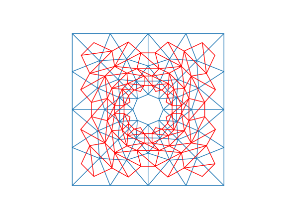
Figure 2: The finite element mesh (blue) and the Lip-mesh (red) built from the centroids of the blue mesh elements.

The continuum Lipschitz set (15) involves an infinite number of constraints since all pairs of points must be considered. We need to find a way to discretize this set. A first option is to bound the damage gradient on every element of the Lip-mesh (17). A second option is to enforce the Lipschitz constraint in between vertices (18-19) . The metric $\mathrm{dist}^{h}(\mbox{\boldmath$x$},\mbox{\boldmath$y$})$ is the shortest path between $x$ and $y$ lying inside $\Delta^{h}$, whereas the discrete metric $\mathrm{dist}^{h+}(\mbox{\boldmath$x$},\mbox{\boldmath$y$})$ forces the path to go along edges (and thus $\mathrm{dist}^{h}(\mbox{\boldmath$x$},\mbox{\boldmath$y$})\leq\mathrm{dist}^{h+}(\mbox{\boldmath$x$},\mbox{\boldmath$y$})$). Finally, another option is to enforce the Lipschitz constraint on each edges (20).

$$\mathcal{L}^{h} =\{d\in D^{h}(\Delta^{h}):\|\nabla d\|\mid_{t}\leq\frac{1}{l},\quad\forall t\in T\}$$ (17)

$$\mathcal{L}^{h1} =\{d\in D^{h}(\Delta^{h}):\lvert d(\mbox{\boldmath$x$})-d(\mbox{\boldmath$y$})\rvert\leq\frac{1}{l}\,\mathrm{dist}^{h}(\mbox{\boldmath$x$},\mbox{\boldmath$y$}),\quad\forall\mbox{\boldmath$x$},\mbox{\boldmath$y$}\in V\}$$ (18)

$$\mathcal{L}^{h2} =\{d\in D^{h}(\Delta^{h}):\lvert d(\mbox{\boldmath$x$})-d(\mbox{\boldmath$y$})\rvert\leq\frac{1}{l}\mathrm{dist}^{h+}(\mbox{\boldmath$x$},\mbox{\boldmath$y$}),\quad\forall\mbox{\boldmath$x$},\mbox{\boldmath$y$}\in V\}$$ (19)

$$\mathcal{L}^{h+} =\{d\in D^{h}(\Delta^{h}):\lvert d(\mbox{\boldmath$x$})-d(\mbox{\boldmath$y$})\rvert\leq\frac{1}{l}\lVert\mbox{\boldmath$x$}-\mbox{\boldmath$y$}\rVert,\quad\forall(\mbox{\boldmath$x$},\mbox{\boldmath$y$})\in E\}$$ (20)

The four options satisfy the following inclusions proven in appendix A:

$$\mathcal{L}^{h}\subset\mathcal{L}^{h1}\subset\mathcal{L}^{h2}=\mathcal{L}^{h+}$$ (21)

We choose the first option because it involves the least number of discrete constraints since the number of element in a mesh is much smaller than the number of edges (or pairs of vertices). Also, compared to $\mathcal{L}^{h+}$ it is less prone to mesh orientation effect because we are checking the Lipschitz constraint on all orientations and not only along along edges (see appendix B). The space-time discrete problem is thus to find at time $t_{n+1}$, the pair $(\mbox{\boldmath$u$},d)$ satisfying

$$(\mbox{\boldmath$u$},d)=\arg\min_{\begin{subarray}{c}\mbox{\boldmath$u$}^{\prime}\in{\cal U}^{h}_{n}\\ d^{\prime}\in{\cal A}^{h}_{n}\cap\mathcal{L}^{h}\end{subarray}}F(\mbox{\boldmath$u$}^{\prime},d^{\prime})$$ (22)

where ${\cal U}^{h}$ indicates the displacement finite element space and ${\cal A}^{h}_{n}$ is given by

$${\cal A}^{h}_{n}=\{d\in D^{h}(\Delta^{h}):d_{n}(\mbox{\boldmath$x$})\leq d(\mbox{\boldmath$x$})\leq 1,\forall\mbox{\boldmath$x$}\in V\}$$ (23)

3.2 Staggered scheme

The optimization problem (22) is not convex with respect to the pair $(u,d)$ but is convex with respect to each variable taken separately. As for the phase-field approach [23], a staggered scheme is used: solve for the displacement with given damage, then solve for damage with given displacement and iterate until convergence. The first minimization is rather standard. The second one is not. It reads

$$d=\arg\min_{\begin{subarray}{c}d^{\prime}\in{\cal A}^{h}_{n}\cap\mathcal{L}^{h}\end{subarray}}F(\mbox{\boldmath$u$},d^{\prime})$$ (24)

where $u$ is known (current iterate). It is a convex minimization problem with cone and second order cone inequality. To solve it we use the cvxopt [5] package, in particular the cp function that can find the minimizer of a general convex function with first and second order cone constraints. An example of Lipschitz projection is given in appendix B for a constructed damage field.

4 The use of bounds for the damage update

The previous section did detail the space discretization as well as the staggered scheme. The damage iterate consists in a convex optimization. It has been observed in the first Lip-field paper [25] that this optimization could be greatly simplified using so-called bounds on the solution. Below, we recall the bound concept and detail how it is implemented in the discrete setting.

4.1 Bounds in the continuum setting

Bounds on the damage solution $d$ have been proposed in the paper [25]. Consider the damage optimization problem

$$d=\arg\min_{\begin{subarray}{c}d^{\prime}\in{\cal A}_{n}\cap\mathcal{L}\end{subarray}}F(\mbox{\boldmath$u$},d^{\prime})$$ (25)

The idea is to first disregard the Lipschitz constraint and compute a local damage update denoted $d_{\mathrm{loc}}$:

$$d_{\mathrm{loc}}=\arg\min_{\begin{subarray}{c}d^{\prime}\in{\cal A}_{n}\end{subarray}}F(\mbox{\boldmath$u$},d^{\prime})\Rightarrow d_{\mathrm{loc}}(\mbox{\boldmath$x$})=\arg\min_{\begin{subarray}{c}d_{n}(\mbox{\boldmath$x$})\leq d^{\prime}\leq 1\end{subarray}}f(\mbox{\boldmath$\epsilon$}(\mbox{\boldmath$u$})\mid_{\mbox{\boldmath$x$}},d^{\prime}),\quad\forall\mbox{\boldmath$x$}\in{\Omega}$$ (26)

In the above, we have use the separability property of the non-regularized optimization with respect to the $d$ variable. The local damage at point $x$ only depends on the strain at that point. Upper and lower bounds are defined as

$$\underline{d}(\mbox{\boldmath$x$}) =\min_{\mbox{\boldmath$y$}\in{\Omega}}\;(d_{\mathrm{loc}}(\mbox{\boldmath$y$})+\frac{1}{l}\mathrm{dist}(\mbox{\boldmath$x$},\mbox{\boldmath$y$}))$$ (27)

$$\overline{d}(\mbox{\boldmath$x$}) =\max_{\mbox{\boldmath$y$}\in{\Omega}}\;(d_{\mathrm{loc}}(\mbox{\boldmath$y$})-\frac{1}{l}\mathrm{dist}(\mbox{\boldmath$x$},\mbox{\boldmath$y$}))$$ (28)

They satisfy

$$d_{n}\leq\underline{d}\leq d_{\mathrm{loc}}\leq\overline{d}\leq 1,\quad\underline{d}\leq d\leq\overline{d}$$ (29)

The proof may be found in [25]. The optimization for $d$ in (25) may thus be replaced by

$$d=\arg\min_{\begin{subarray}{c}d^{\prime}\in\overline{{\cal A}}_{n}\cap\mathcal{L}\end{subarray}}F(\mbox{\boldmath$u$},d^{\prime})$$ (30)

where

$$\overline{{\cal A}}_{n}=\{d\in L^{\infty}(\Omega):\underline{d}\leq d\leq\overline{d}\}\subset{\cal A}_{n}$$ (31)

It is clear that at any point for which the bounds are equal, the local damage update is optimal:

$$\underline{d}(\mbox{\boldmath$x$})=\overline{d}(\mbox{\boldmath$x$})\Rightarrow d(\mbox{\boldmath$x$})=d_{\mathrm{loc}}(\mbox{\boldmath$x$})$$ (32)

The bounds computation may thus potentially drastically reduce the effort for the damage optimization by locating the subdomain over which the local update needs to be further corrected. The subdomain is an upper-bound for the zone over which the Lipschitz constraint will be active.

4.2 Bounds in the discrete setting

First, a local update may be computed at each vertex

$$d_{\mathrm{loc}}(\mbox{\boldmath$x$})=\arg\min_{\begin{subarray}{c}d_{n}(\mbox{\boldmath$x$})\leq d^{\prime}\leq 1\end{subarray}}f(\mbox{\boldmath$\epsilon$}(\mbox{\boldmath$u$})\mid_{\mbox{\boldmath$x$}},d^{\prime}),\quad\forall\mbox{\boldmath$x$}\in V$$ (33)

Then, we propose to compute the following bounds

$$\underline{d}(\mbox{\boldmath$x$}) =\min_{\mbox{\boldmath$y$}\in V}\;(d_{\mathrm{loc}}(\mbox{\boldmath$y$})+\frac{1}{l}\mathrm{dist}^{h+}(\mbox{\boldmath$x$},\mbox{\boldmath$y$})),\quad\forall\mbox{\boldmath$x$}\in V$$ (34)

$$\overline{d}(\mbox{\boldmath$x$}) =\max_{\mbox{\boldmath$y$}\in V}\;(d_{\mathrm{loc}}(\mbox{\boldmath$y$})-\frac{1}{l}\mathrm{dist}^{h+}(\mbox{\boldmath$x$},\mbox{\boldmath$y$})),\quad\forall\mbox{\boldmath$x$}\in V$$ (35)

The definition above seems to indicate that $O(n^{2})$ operations are required, where $n$ is the number of vertices in $V$. Fortunately, an algorithm inspired from Dijkstra’s algorithm [9] reduces the effort to $O(n\log n)$ operations. It is detailed in the appendix C. At any vertex, the bounds satisfy similar inequalities than the bounds in the continuum setting (see proof in the appendix D):

$$d_{n}(\mbox{\boldmath$x$})\leq\underline{d}(\mbox{\boldmath$x$})\leq d_{\mathrm{loc}}(\mbox{\boldmath$x$})\leq\overline{d}(\mbox{\boldmath$x$})\leq 1,\quad\underline{d}(\mbox{\boldmath$x$})\leq d^{+}(\mbox{\boldmath$x$})\leq\overline{d}(\mbox{\boldmath$x$}),\quad\forall\mbox{\boldmath$x$}\in V$$ (36)

where

$$d^{+}=\arg\min_{\begin{subarray}{c}d^{\prime}\in{\cal A}^{h}_{n}\cap\mathcal{L}^{h+}\end{subarray}}F(\mbox{\boldmath$u$},d^{\prime})$$ (37)

Unfortunately, the bounds do not bracket the solution $d$ from we are after (24) but another solution defined by (37). The reason for this discrepancy is that we have chosen the metric $\mathrm{dist}^{h}$ instead of $\mathrm{dist}$ to compute the bounds because the former gives an extremely simple algorithm. To take into account the discrepancy, we use the following scheme.

• Step 1: Compute the bounds (34)-(35) using the algorithm given in the appendix C.

• Step 2: Initialize $V^{l}$ to the set of vertices for which $\underline{d}(\mbox{\boldmath$x$})=\overline{d}(\mbox{\boldmath$x$})$ and define $T^{l}$ as the set of elements connected to nodes only in $V^{l}$.

• Step 3: Solve

  $$d=\arg\min_{\begin{subarray}{c}d^{\prime}\in\overline{{\cal A}}^{h}_{n}\cap\overline{\mathcal{L}}^{h}\end{subarray}}F(\mbox{\boldmath$u$},d^{\prime})$$ (38)

  where

  $$\overline{{\cal A}}^{h}_{n} =\{d\in D^{h}(\Delta^{h}):d(\mbox{\boldmath$x$})=d_{\mathrm{loc}}(\mbox{\boldmath$x$}),\forall\mbox{\boldmath$x$}\in V^{l}\text{\ and\ }d_{n}(\mbox{\boldmath$x$})\leq d(\mbox{\boldmath$x$})\leq 1,\forall\mbox{\boldmath$x$}\in V\setminus V^{l}\}$$ (39)

  $$\overline{\mathcal{L}}^{h} =\{d\in D^{h}(\Delta^{h}):\|\nabla d\|\mid_{t}\leq\frac{1}{l},\quad\forall t\in T\setminus T^{l}\}$$ (40)

• Step 4: If $d\in\mathcal{L}^{h}$ end, else remove the element for which $\|\nabla d\|>1/l$ from $T^{l}$ and remove its node from $V^{l}$, go to Step 3.

If the bounds were associated to the true solution, step 4 would end directly. In the numerical experiments we have noticed that Step 3 was repeating itself only on rare occasions, showing that the discrepancy is not too detrimental.

5 Simulation results

All examples are computed using plane strain assumption. The meshes and the python scripts used for are all the examples are open-source and may be downloaded from https://gitlab.com/c4506/lipfield. All examples are treated with the symmetrical model ($\beta=0$) except for the shear test which is treated with both the symmetrical ($\beta=0$) and asymmetrical ($\beta=1$) models.

For all examples, the mesh is built using the open-source gmsh software [15]. Regarding the Lip-mesh, it is constructed using the open-source Triangle software [32] available at https://www.cs.cmu.edu/~quake/triangle.research.html along with a python interface available at https://github.com/pletzer/pytriangle.

5.1 Plate with a hole

As a first example, we pull the sides of a square domain with imposed displacement. The square is pierced at its center by with a circular hole. The geometric and material parameters used are reported on table 1. The material parameters are chosen generically for this first example since we are just trying here to assess the method qualitatively.

units $L$ $R$ mm 2 0.2

$E$ $\nu$ $l$ $Y_{\mathrm{c}}$ $\eta$ 1 MPa 0.2 0.2 mm 1 MPa 0.1

Table 1: Hole in a plate: geometrical parameters (left), material parameters (right).

The mesh is unstructured and parametrized by the size of $h$ the edge of the triangles on the boundary of the square and the circular hole. Results are reported on figure 3. On the top left, we have the load/displacement curve. We have first an elastic loading, until the stored energy is sufficient to trigger damage. We then have a short softening phase, where the damage start to grow gently at two symmetric locations at the top and bottom of the hole, followed by an abrupt release of strain energy during which the damage zones develop in two cracks propagating up to the boundary of the plate. This setting clearly shows a strong instability, and the equilibrium path is discontinuous under displacement loading. To improve on that, we could consider another control mechanism in order to follow the snap-back behavior.

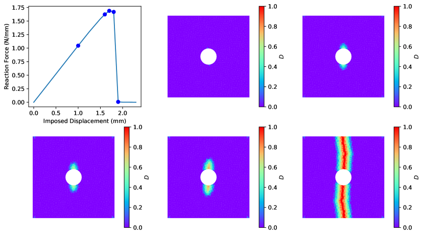
Figure 3: Load displacement curve and damage field for mesh 2.

mesh	$L/h$	vertices	faces
mesh 1	16	1524	2896
lip-mesh 1		2896	5476
mesh 2	32	5640	10980
lip-mesh 2		10980	21308
mesh 3	64	19333	38070
lip-mesh 3		38070	74947

Table 2: Mesh parameters for the convergence analysis.

Figure 4: Convergence analysis: top damage field, below $u_{x}$, $\epsilon_{xx}$ extracted from the white line for different meshes, at the end of the simulation.

Figure 4 reports on a convergence analysis. All the parameters are kept identical except for the mesh density which is increased as show on table 2. The damage field is plotted on the top row, with the finer mesh on the right. The two damage zones take the shape of a vertical band, of thickness close to $2l$ where the damage reach $1$ at the center of the band. The elements for which $d$ reaches $1$ have of course no stiffness and could be identified as cracks. On the coarsest mesh, the band is not perfectly straight due to the unstructured nature of the mesh. As the mesh is refined, while keeping $l$ constant, more and more elements fit into the thickness of the band which appears straighter and straighter while the damage field is described with more and more precision. On the middle row of the figure, we report the damage field, for each mesh, along the white line represented on the top row. The white line is perpendicular to the crack, and the damage field clearly reaches $1$ on the crack, and reduces at a slope fixed by the Lipschitz constraint away from the crack. The thickness of the damaged zone clearly converges quickly toward the value of $2l$. We plot for each mesh the damage field as seen by the mechanical problem (constant per mesh element) and the damage field as seen by the Lip-field problem (linear on each element of the Lip-Mesh). Note that both fit very well to the expected wedge shape imposed by the Lip-field constraint. This means that in absence of the constraint, the damage would be zero everywhere away from a strip of 1 element thickness, reproducing the classical mesh dependency of the result for a local damage model. The last row of the figure reports, along the same line, the displacement and the strain field. Notice how the displacement clearly displays a sharp jump over the thickness of a single element, reproducing the result that would have been obtained if we would have inserted a sharp crack in the mesh. The deformation component $\epsilon_{xx}$ is also plotted and the expected Dirac-like function shape is captured.

5.2 Comparison with a Griffith analysis

The geometry described in figure 5 is used to study crack propagation. This geometry is inspired from the classic TDCB (tapered double cantilever beam) shape that insures a stable crack growth relative to an increasing displacement loading.

Figure 5: TDCB geometry definition.

units	$L_{1}$	$L_{2}$	$L_{3}$	$L_{4}$	$H_{1}$	$H_{2}$	$H_{3}$	$H_{4}$	$R$
mm	100	12	20	24	70	90	24	5	4

Table 3: TDCB geometrical parameters.

$E$	$\nu$	$K_{I_{c}}$	$\eta$
3500 $\mathrm{MPa}$	0.32	1.4 $\mathrm{MPa\sqrt{m}}$	0.1

Table 4: TDCB material parameters.

The dimensions defining the geometry are given in table 3. The TDCB specimen is loaded by a linearized rigid body motion on the boundary of the two holes. The bottom hole has its center fixed, while it is free to rotate around the $z$ axis. The top hole is free to rotate around the $z$ axis, its center is fixed on the $x$ axis, while its motion on the $y$ axis is imposed and is the loading parameter $u$. We make the classical plane-strain and small-strain assumption. The material is described with the coefficients given in table 4, where $E$, $\nu$ and $K_{I_{c}}$ denote respectively, the Young Modulus, Poisson ratio and the critical mode I stress intensity factor. Upon loading, a crack is expected to develop at the notch tip, and propagate along the middle axis of the TDCB specimen, which will be called the crack path. For a first validation of the Lip-field approach for brittle damage we will compare our results with a linear elastic fracture mechanics analysis, using a Griffith criteria.

Griffith Analysis

According to the Griffith criterion, the crack should propagate if the elastic energy release rate per unit of crack length $G$ is equal to $G_{\mathrm{c}}$, where $G_{\mathrm{c}}$ is a material parameter: the critical energy release rate. Under plane strain assumption, for isotropic-elastic material, we have

$$G_{\mathrm{c}}=\frac{1-\nu^{2}}{E}{K_{I_{c}}}^{2}$$ (41)

In order to compute the load-displacement ($F(u)$) and the crack-length ($a(u)$) under Griffith assumption, we applied the following approach. The mesh is constructed in two symmetrical-part along the crack-path, so that the nodes on the crack-line are regularly spaced and we denote by $h$ the spacing between two nodes. The mesh of the upper part and the mesh of the lower part are disconnected, but the nodes of each part are at the same geometrical positions on the crack-path. The nodes are connected using a Lagrange multiplier to enforce the same displacement on both part at each of these node, on the section of the crack-path to the right of the actual crack. With this setting, we can easily compute the equilibrium displacement field $\mathbf{u}$ and the strain energy $e$ in the TDCB specimen using the standard finite element method, for different crack-length and a unit displacement $u$. For each crack length $a$, corresponding to a number of unconnected nodes on the crack path, we can compute the energy release-rate $G_{1}(u)$ for the unit displacement, by using a first order Taylor expansion:

$$G_{1}(a)=\frac{e_{1}(a+h)-e_{1}(a-h)}{2h}$$ (42)

where $e_{1}(a)$ is the strain energy at equilibrium for the crack of length $a$ and a imposed displacement $u=1$. Since $G$ is clearly a quadratic function of $u$, we can compute for each value of $a$ the value of $u_{c}$ and then $f_{c}$ for which $G=G_{c}$, and plot the $F(u)$ and $a(u)$ curves for the case of Griffith analysis.

Lip-field Analysis

In order to compare Griffith analysis and Lip-field, we need to set up the parameter of the damage model in order to be energetically equivalent to Griffith. Assuming that when the damage localize into a shape of a crack, and that $d$ saturates the Lipschitz constraint and reaches $1$ on the crack path. We can approximate the $d(y)$ function on a line perpendicular to the crack path with a triangular profile of slope $1/l$: $d(y)=\frac{\max(l-\lvert y\rvert,0)}{l}$, where $y$ is the distance to the crack path. We can then evaluate the energy dissipated per unit of crack advance by $G_{\mathrm{c}}=Y_{\mathrm{c}}\int_{-l}^{l}h(d(y))dy=4Y_{\mathrm{c}}l$. In the simulations, we set $l$ so that we have enough elements in the band to represent the crack (typically $l=5h$), and then set $Y_{\mathrm{c}}=G_{\mathrm{c}}/(4l)$.

The comparison between Griffith and Lip-field is given on figure 6 where we report the reaction on the anchoring circle and the crack length as a function of the imposed displacement, for both Griffith and Lip-field analysis.

Figure 6: Griffith/Lip-field comparison.

In both cases, after reaching a critical displacement, the reaction drops in a controlled way, while the crack advance at a pace proportional to the imposed displacement pace, until the crack length cover roughly three quarters of its maximum length. After that, the pace of crack progressively slows down, until it reaches the right boundary of the sample. The results compare well: we observe the same critical displacement, and the same speed between Griffith and Lip-field, even if we have a slight difference in dissipated energy and crack tip position. A more extensive study is beyond the scope of this paper, but we have already a good confirmation of the ability of Lip-field to reproduce Griffith physics.

5.3 Shear test

In the next example, we perform a shear test on the geometry given in figure 7. A square sample of length $2L=1\mathrm{mm}$ is initially cut by a line, from the left boundary to the center. This is meant to represent an initial crack. The bottom of the square is fixed, while the top has its displacement fixed to 0 in the $y$ direction and imposed in the $x$ direction. This benchmark is popular in the phase-field literature [36]. The material properties are given in table 5, and $Y_{\mathrm{c}}$ is computed to obtain energetic equivalence as discussed in previous subsection ($Y_{\mathrm{c}}=G_{c}/(4l)$). The parameter $\eta$ is set to $0.1$. The two parameters $h_{0}$ and $h_{1}$ are the target edge sizes for the meshing tool in the coarse and fine zone, respectively, as indicated in figure 7. The extent of the fine zone has been determined thanks to an initial run on a coarse mesh in order to identify the zone in which the damage localizes into a crack. The parameters for the two meshes used for this example are given in table 6.

$E$	$\nu$	$l$	$G_{c}$	$\eta$
210000 $\mathrm{MPa}$	0.2	0.015$\mathrm{mm}$	2.7 $\mathrm{MPa/mm}$	0.1

Table 5: Shear test material parameters.

Figure 7: From left to right : shear test geometry and boundary conditions definition, mesh parameter for the symmetric case and the asymmetric case

mesh	$h_{0}$	$h_{1}$	vertices	faces
symmetric	1/8 mm	1/128 mm	26656	53311
asymmetric	1/8 mm	1/128 mm	11343	22685

Table 6: Mesh parameters for the shear test.

We report on figure 8, the load/displacement curve, as well as the damage field, at different stages of the loading represented by dots on the curve.

Figure 8: Shear test: symmetric traction/compression. Top left: load displacement curve. From left to right and top to bottom, damage field at the corresponding dot on the curve.

After an elastic phase, damage starts to develop at the initial crack tip when $Y$ reach $Y_{\mathrm{c}}$. The reaction force on the top edge of the square then rapidly drops as two cracks develop in a symmetric pattern starting from the crack tip until the reaction reaches zero when the two cracks reach the right boundary. Notice how cracks gradually turn while advancing until they reach the right boundary. This result could not have been obtained with Griffith theory alone: one should have had some model to predict the crack advance direction. As in the phase field or in the TLS approach, no additional assumption is needed to account for crack direction change. It is the minimization of the energy that naturally drives the crack. This example also shows that the Lip-field approach is able to represent branching cracks. The crack pattern and the load/displacement curve is consistent with published results [36], [2]. These results are however unrealistic considering that the top crack develops in compression, so that when $d$ reaches $1$, we have overlapping of the lips of the crack. This issue is not new. In order to avoid this behavior, we need an asymmetric traction/compression model, where the damage function $g(d)$ only affects the traction part of the strain energy as discussed in part 2. The simulations have been re-run using this change in and on a mesh adapted for the expected crack path. The results are reported on figure 9.

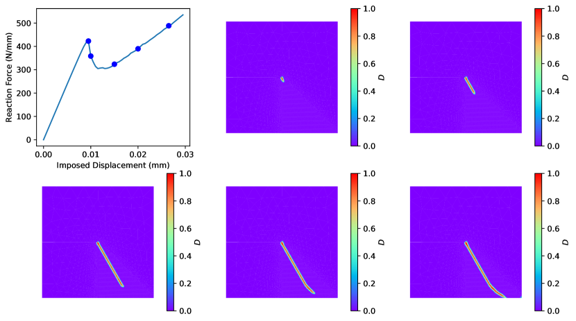
Figure 9: Shear test: Asymmetric traction/compression. Top left: load displacement curve. From left to right, top to bottom damage field at the corresponding dot on the curve.

Up to the point where the damage starts to localize at the initial crack tip, the results are similar to the symmetric case. Then, when the reaction force starts to decrease, the damage zone localizes in only one crack, on the bottom side of the square, propagating first along a straight line until it gets close to the bottom fixed boundary and the reaction force reaches a local minimum. Then it starts to turn while the reaction start growing again, in contrast with the previous case. Notice how the gradient of the damage in the normal direction to the boundary ($\mathbf{\nabla}d\cdot\mathbf{n}$) is not zero when the crack reaches the boundary. This is in sharp contrast with results obtained in the framework of the phase field theory where the strong form imposes $\mathbf{\nabla}d\cdot\mathbf{n}=0$.

5.4 Two edge cracks

For the last example, we reproduce another popular test case, two edge cracks, presented and solved for example in [18]. Starting from a square sample, two horizontal initial cracks are cut out of the sample, one on each side but at different heights (see figure 10).

Figure 10: Two edge cracks, geometric description, boundary condition and meshing parameters.

Table 7 reports the geometrical, material and mesh parameters used for the simulation. The damage model is here symmetric with regards to traction and compression. As in the previous case, we use two parameters $h_{0}$ and $h_{1}$ to control the mesh density. We have a finer mesh in the zone where the damage is expected to propagate (light gray on figure 10).

Geometrical parameters:	Mesh parameters:
$L$ $C$ $a$ mm 1 0.95 0.2	$h_{0}$ $h_{1}$ vertices faces 0.025mm 0.003125mm 26338 52675
	Material parameters:
	$E$ $\nu$ $l$ $Y_{\mathrm{c}}$ $\eta$ 1 MPa 0.2 0.01 mm 1 MPa 0.1

Table 7: Two edge cracks geometrical, mesh and material parameters.

The square is fixed at the bottom while the top edge is pulled in displacement control in the $y$ direction. Results are reported on figure 11.

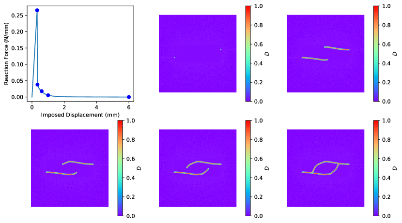
Figure 11: Two edge cracks, top left: load displacement curve. From left to right, damage field at the corresponding dot on the curve.

We first have a quasi elastic phase where the damage is confined to the two initial crack tips until we reach a critical load. Beyond the critical load, the two damaged zones start to grow, localizing into two cracks that start to propagate, forming a pattern that maintains a central symmetry with regard to the center of the square, while the reaction force on the top boundary quickly drops. The left crack propagates to the right with a slight angle toward the bottom while the right crack propagates to the left with a slight angle toward the top, until both reaches the vertical axis of symmetry of the square. After that, the path of both crack starts to curve toward the horizontal axis of symmetry of the square until both crack tips finally merge. Note that the damage at a distance larger that $l$ from the place where $d$ reaches its maximum is exactly zero. There is no damage away from the localization zone. The crack pattern obtained is similar to what is observed in previous work.

6 Conclusions and future work

The paper described a first two dimensional finite element implementation of the Lip-field approach for brittle fracture with symmetric and asymmetric damage models in tension/compression. This follows introduction of the Lip-field approach and its one dimensional implementation reported in [25].

A variety of examples have been treated demonstrating the independence of the crack path from the mesh, and good convergence properties. A comparison with the Griffith model has also been provided and shows good correlation.

The main originality of the Lip-field approach is to be found in the way the local equations are regularized. Instead of adding a damage gradient contribution to the incremental potential, as in the phase-field approach, the damage is constrained to be Lipschitz continuous under a given length. This approach has some advantages compared to phase-field. The main one is that we can use a local minimization as a starting point. Then, using the bounding technique, construct patches where the Lipschitz constraint needs to be enforced. This strongly reduces the number of elements where we must explicitly minimize under non local constraint the potential with respect to the $d$ field in the staggered scheme. This naturally leads to an algorithm where the cost of the minimization on $d$ can be much lower than the computation of the equilibrium at fixed $d$.

Encouraged by these results, we plan to extend the method in the following directions in the future:

• Softening plasticity. This would open a large array of potential applications. We previously demonstrated in the 1D case that the approach was sound and gave interesting results. Extending this approach to two dimensions should not be difficult and should be a low hanging fruit for the method.

• Mesh refinement. It is clear from the examples, that as well as phase field, quite fine meshes are necessary to capture the shape of the damaged zone. A logical step toward better results would be to allow automatic mesh refinement to capture the localized damage zone at low cost during a simulation. Strategies to transfer the $d$ field from one mesh to another, while fulfilling the Lipschitz constraints need to be developed.

• Improving the resolution step for the $d$ field. Even if the non-local part of the constrained minimization can be done on relatively small patches of the mesh, the resolution algorithm that we used so far might not be optimal. We indeed rely on interior point method which has the inconvenient to prevent easy use of good starting point for the minimization, because of the centering step typical of such family of methods. Considering that we could obtain good starting points, iterative projection methods might be a better choice for our specific problem. Taking more advantage of the fact that the objective function is separable in $d$ should also help finding a faster algorithm.

• Dynamics. It would be interesting to apply the method in a dynamical setting. That would be the occasion to study cases where the crack path become much more complicated.

• Finally, we could of course move to three-dimensional problem. The only difficulties are technical: the problems to solve will become big very quickly, and parallel implementation will be needed. A 3 dimensional implementation would need to take advantage of all the improvements cited previously in order to give results in a reasonable computational time.

Appendices

Appendix A Proof of (21) recalled below

$$\mathcal{L}^{h}\subset\mathcal{L}^{h1}\subset\mathcal{L}^{h2}=\mathcal{L}^{h+}$$ (43)

To prove the first inclusion, consider the shortest path inside $\Delta^{h}$ linking two vertices. This path is given by a continuous curve $\mbox{\boldmath$z$}(s),s\in[0,1]$. Suppose now $d\in\mathcal{L}^{h}$, we thus have

$$-\frac{1}{l}\lVert\frac{\mbox{\, $\mathrm{d}$}\mbox{\boldmath$z$}}{\mbox{\, $\mathrm{d}$}s}\rVert\leq\nabla d\cdot\frac{\mbox{\, $\mathrm{d}$}\mbox{\boldmath$z$}}{\mbox{\, $\mathrm{d}$}s}\leq\frac{1}{l}\lVert\frac{\mbox{\, $\mathrm{d}$}\mbox{\boldmath$z$}}{\mbox{\, $\mathrm{d}$}s}\rVert$$ (44)

Integrating the above with respect to $s\in[0,1]$ gives the result. The second inclusion in (21) is a direct consequence of the fact that

$$\mathrm{dist}^{h}(\mbox{\boldmath$x$},\mbox{\boldmath$y$})\leq\mathrm{dist}^{h+}(\mbox{\boldmath$x$},\mbox{\boldmath$y$}),\quad\forall\mbox{\boldmath$x$},\mbox{\boldmath$y$}\in V$$ (45)

Finally, regarding the equality in (21), we first note that $\mathcal{L}^{h2}\subset\mathcal{L}^{h+}$ since $\mathcal{L}^{h2}$ checks all pairs of vertices whereas $\mathcal{L}^{h+}$ only checks pairs of vertices forming an edge. And for two vertices $x$, $y$ forming an edge, we have $\mathrm{dist}^{h+}(\mbox{\boldmath$x$},\mbox{\boldmath$y$})=\lVert\mbox{\boldmath$x$}-\mbox{\boldmath$y$}\rVert$. Then, we prove $\mathcal{L}^{h+}\subset\mathcal{L}^{h2}$ using similar arguments as the one used to prove the first inclusion.

Appendix B An example of Lipschitz projection

As an example we consider a damage field $d$ that does not satisfy the Lipschitz constraint of length scale $l$, and we wish to project onto $\mathcal{L}$ while minimizing the $L^{2}(\Omega)$ distance to $d$. We define the distance between two field as the usual distance in $L^{2}(\Omega)$ as $w(d_{1},d_{2})=(\int_{\Omega}(d_{1}-d_{2})^{2}d{\Omega})^{1/2}$. The projection of $d$ onto $\mathcal{L}$ is defined by $\pi_{\mathcal{L}}(d)=\arg\min_{d^{\prime}\in\mathcal{L}}w(d,d^{\prime})$.

Let $\Omega$ be a square of length $L$, centered at point at the origin of the 2D plane. We define a field $d\in L^{2}(\Omega)$ which is not in $\mathcal{L}$ as:

$$d(x,y)=\max\left(1-r(x,y)/\bar{l},0\right)$$ (46)

where $r$ is the distance to the origin and $\bar{l}<l$ is a constant actually corresponding to the Lipschitz constant of the field $d$. In this case we can easily compute the projection on $\mathcal{L}$ as:

$$\pi_{\mathcal{L}}(d)=\max\left(\sqrt[3]{\left(\frac{\bar{l}}{l}\right)^{2}}-r(x,y)/l,0\right)$$ (47)

Now we want to check the precision of the discretized projection on different mesh, using either the $\mathcal{L}^{h}$ or $\mathcal{L}^{h+}$ constraint. For the computation, we use $l=1$ and $\bar{l}=1/4$ and a series of structured meshes parametrized by $L/h$, where $h$ is the length of the edges along the $x$ axis.

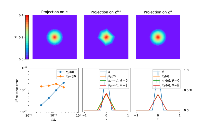
Figure 12: Convergence of the discrete lip projection. Top, from left to right: $\pi_{\mathcal{L}}(d)$ interpolated on the mesh, $\pi_{\mathcal{L}^{h+}}(d)$ and $\pi_{\mathcal{L}^{h+}}(d)$. Bottom: from left to right, convergence analysis, cut of $\pi_{\mathcal{L}^{h+}}(d)$ and $\pi_{\mathcal{L}^{h}}(d)$ along the horizontal line ($\theta=0$) and the diagonal ($\theta=\frac{\pi}{4}$), compared to $d$ and $\pi_{\mathcal{L}}(d)$ .

Results are reported on figure 12. On the top row, the map of $\pi_{\mathcal{L}}(d)$, $\pi_{\mathcal{L}^{h+}}(d)$ and $\pi_{\mathcal{L}^{h}}(d)$ are plotted for $h/L=1/32$. On the bottom row, starting from the left, we plotted first the $L^{2}(\Omega)$ relative error norm for $\pi_{\mathcal{L}^{h+}}(d)$ and $\pi_{\mathcal{L}^{h}}(d)$ as a function of $h/L$, followed by extraction along lines passing trough the origin at different angle $\theta$ from the $x$ direction the values of $d$, and its different projections computed on mesh $h/L=1/32$.

The map of $\pi_{\mathcal{L}^{h}}(d)$ is very close to the map of $\pi_{\mathcal{L}}(d)$, This is confirmed by the cut plot, and the convergence analysis where the error scale linearly with $h$. On the contrary, refining the mesh for $\pi_{\mathcal{L}^{h+}}(d)$ does not improve significantly the results. Indeed, if we get a correct estimate of the maximum value, the slope of the projection slightly change depending on the direction, in a manner strongly dependent with the alignment of the direction with the existing edges in the mesh.

Appendix C Dijkstra based algorithm to compute the bounds (34) and (35)

The set $V$ of vertices in the $\Delta^{h}$ mesh is partitioned into a set of trial and final vertices, denoted $V_{\mathrm{trial}}$ and $V_{\mathrm{final}}$, respectively. At any step in the algorithm, we have $V_{\mathrm{trial}}\cup V_{\mathrm{final}}=V$ and $V_{\mathrm{trial}}\cap V_{\mathrm{final}}=\emptyset$. The algorithm starts with $V_{\mathrm{final}}$ empty and ends when $V_{\mathrm{trial}}$ is empty. The bounds are initialize to $d_{\mathrm{loc}}$ given by (33). The upper bound $\overline{d}$ is obtained by

• Step 0: $V_{\mathrm{trial}}=V$, $V_{\mathrm{final}}=\emptyset$, $\forall v\in V:\overline{d}(v)\leftarrow d_{\mathrm{loc}}(v)$

• Step 1: $v^{*}=\arg\max_{\begin{subarray}{c}v\in V_{\mathrm{trial}}\end{subarray}}\overline{d}(v)$, $V_{\mathrm{trial}}\leftarrow V_{\mathrm{trial}}\setminus\{v^{*}\}$, $V_{\mathrm{final}}\leftarrow V_{\mathrm{final}}\cup\{v^{*}\}$

• Step 2: $\forall v\in V_{\mathrm{trial}}$ such that $(v,v^{*})\in E:\overline{d}(v)\leftarrow\max(\overline{d}(v),\overline{d}(v)-\lVert v-v^{*}\rVert/l)$

• Step 3: If $V_{\mathrm{trial}}=\emptyset$ end, else go to Step 1.

Similarly, one may build the lower bound $\underline{d}$ from the following:

• Step 0: $V_{\mathrm{trial}}=V$, $V_{\mathrm{final}}=\emptyset$, $\forall v\in V:\underline{d}(v)=d_{\mathrm{loc}}(v),$

• Step 1: $v^{*}=\arg\min_{\begin{subarray}{c}v\in V_{\mathrm{trial}}\end{subarray}}\underline{d}(v)$, $V_{\mathrm{trial}}\leftarrow V_{\mathrm{trial}}\setminus\{v^{*}\}$, $V_{\mathrm{final}}\leftarrow V_{\mathrm{final}}\cup\{v^{*}\}$

• Step 2: $\forall v\in V_{\mathrm{trial}}$ such that $(v,v^{*})\in E:\underline{d}(v)\leftarrow\min(\underline{d}(v),\underline{d}(v)+\lVert v-v^{*}\rVert/l)$

• Step 3: If $V_{\mathrm{trial}}=\emptyset$ end, else go to Step 1.

To unsure $O(nlog(n))$ efficiency, where $n$ is the size of $V$, the set $V_{\mathrm{trial}}$ is maintained as a descending sorted list according to the value of $\underline{d}(v)$ (resp. $\overline{d}$). Step 1 is reduced to take the first (resp. the last) of the list, and at step 2, all the $v$ for which $\underline{d}(v)$ (resp. $\overline{d}(v)$) have been updated must be relocated in the list so that the ordering is maintained.

Appendix D Proof of the bounds in the discrete setting

eq:disbound We prove (36) recalled below

$$d_{n}(\mbox{\boldmath$x$})\leq\underline{d}(\mbox{\boldmath$x$})\leq d_{\mathrm{loc}}(\mbox{\boldmath$x$})\leq\overline{d}(\mbox{\boldmath$x$})\leq 1,\quad\underline{d}(\mbox{\boldmath$x$})\leq d^{+}(\mbox{\boldmath$x$})\leq\overline{d}(\mbox{\boldmath$x$}),\quad\forall\mbox{\boldmath$x$}\in V$$ (48)

The first relation is a direct consequence of the initialization of $\underline{d}$ and $\overline{d}$ at $d_{\mathrm{loc}}$ and the use of Step 2 of the algorithm (detailed in the previous appendix). The second relation in (48) amounts to prove that the optimal solution cannot be outside the bounds. The same argument as in in the continuum setting [25] may be used. The objective function is a sum of convex functions in $d$ at every vertex of the $\Delta^{h}$ mesh whose minimum is $d_{\mathrm{loc}}$. If the optimal solution lies outside the bound, we can build a better solution by projecting it on the bounds (the minimum or maximum of Lipschitz functions stays Lipschitz). This proves the second part of (48).

References

- [1] E. Aifantis. On the microstructural origin of certain inelastic models. Journal of Eng. Mat. and Tech., 106(4):326–330, 1984.
- [2] G. Allaire, F. Jouve, and N. Van Goethem. Damage and fracture evolution in brittle materials by shape optimization methods. Journal of Computational Physics, 230(12):5010–5044, 2011.
- [3] M. Ambati, T. Gerasimov, and L. De Lorenzis. Phase-field modeling of ductile fracture. Comp. Mech., 55(5):1017–1040, 2015.
- [4] H. Amor, J.-J. Marigo, and C. Maurini. Regularized formulation of the variational brittle fracture with unilateral contact: Numerical experiments. J. of the Mech. and Phys. of Sol., 57(8):1209–1229, 2009.
- [5] M. Andersen and L. Vandenberghe. The cvxopt linear and quadratic cone program solvers. https://cvxopt.org/.
- [6] G. Barenblatt. The mathematical theory of equilibrium cracks in brittle fracture. Advances in Applied Mechanics, 7:55–129, 1962.
- [7] B. Bourdin, G. Francfort, and J.-J. Marigo. Numerical experiments in revisited brittle fracture. J. of the Mech. and Phys. of Sol., 48(4):797–826, 2000.
- [8] B. Bourdin, G. Francfort, and J.-J. Marigo. The variational approach to fracture. J. of Elas., 91(1-3):5–148, 2008.
- [9] E. Dijkstra. A note on two problems in connexion with graphs. Numer. Math., 1:269––271, 1959.
- [10] D. Dugdale. The phenomena of rupture and flow in solids. Phil. Trans. R. Soc. Lond. Ser. A, Math. Phys. Sci., 221:163–198, 1921.
- [11] D. Dugdale. Yielding of steel sheets containing slits. J. of the Mech. and Phys. of Sol., 8:100–104, 1960.
- [12] G. Francfort and J.-J. Marigo. Revisiting brittle fracture as an energy minimization problem. J. of the Mech. and Phys. of Sol., 46:1319–1412, 1998.
- [13] M. Frémond and B. Nedjar. Damage, gradient of damage and principle of virtual power. Int. J. of Sol. and Struct., 33(8):1083–1103, 1996.
- [14] P. Germain, P. Suquet, and Q. S. Nguyen. Continuum thermodynamics. ASME Journal of Applied Mechanics, 50:1010–1020, Dec. 1983.
- [15] C. Geuzaine and J.-F. Remacle. Gmsh: A 3-d finite element mesh generator with built-in pre-and post-processing facilities. International journal for numerical methods in engineering, 79(11):1309–1331, 2009.
- [16] B. Halphen and Q.-S. Nguyen. Sur les matériaux standards généralisés. Journal de Mécanique, 14(1):39–63, 1975.
- [17] A. Javili, R. Morasata, E. Oterkus, and S. Oterkus. Peridynamics review. Math. and Mech. of Solids, 24(11):3714–3739, 2018.
- [18] P. O. Judt and A. Ricoeur. Crack growth simulation of multiple cracks systems applying remote contour interaction integrals. Theoretical and Applied Fracture Mechanics, 75:78–88, 2015.
- [19] A. Karma, D. Kessler, and H. Levine. Phase-field model of mode III dynamic fracture. Phys. Rev. Lett., 87(4):045501, 2001.
- [20] C. Kuhn and R. Müller. A continuum phase field model for fracture. Eng. Frac. Mech., 77(18):3625–3634, 2010.
- [21] E. Lorentz. A mixed interface finite element for cohesive zone models. Computer Methods in Applied Mechanics and Engineering, 198(2):302–317, 2008.
- [22] E. Lorentz and S. Andrieux. Analysis of non-local models through energetic formulations. Int. J. of Sol. and Struc., 40:2905–2936, 2003.
- [23] C. Miehe, M. Hofacker, and F. Welschinger. A phase field model for rate-independent crack propagation: Robust algorithmic implementation based on operator splits. Computer Methods in Applied Mechanics and Engineering, 199(45-48):2765–2778, nov 2010.
- [24] C. Miehe, F. Welschinger, and M. Hofacker. Thermodynamically consistent phase-field models of fracture: Variational principles and multi-field FE implementations. Int. J. For Num. Meth. in Eng., 83(10):1273–1311, 2010.
- [25] N. Moës and N. Chevaugeon. Lipschitz regularization for softening material models: The Lip-field approach. Comptes Rendus - Mecanique, 349(2):415–434, mar 2021.
- [26] N. Moës, C. Stolz, P.-E. Bernard, and N. Chevaugeon. A level set based model for damage growth : The thick level set approach. Int. J. For Num. Meth. in Eng., 86:358–380, 2011.
- [27] Q.-S. Nguyen and S. Andrieux. The non-local generalized standard approach: A consistent gradient theory. Cptes rend. Acad. des sciences: Mécanique, physique, chimie, astronomie, 333:139–145, 2005.
- [28] R. Peerlings, M. Geers, R. De Borst, and W. Brekelmans. A critical comparison of nonlocal and gradient-enhanced softening continua. Int. J. of Sol. and Struc., 38(44-45):7723–7746, 2001.
- [29] G. Pijaudier-Cabot and Z. Bazant. Non-local damage theory. J. of Eng. Mech., 113:1512–1533, 1987.
- [30] C. Z. Schreyer H. One-dimensional softening with localization. J. of Appl. Mech., 53:891–979, 1986.
- [31] A. Seagraves and R. Radovitzky. Advances in cohesive zone modeling of dynamic fracture. In: Dynamic failure of materials and structures, Springer, pages 349–405, 2009.
- [32] J. R. Shewchuk. Applied Computational Geometry Towards Geometric Engineering. Triangle: Engineering a 2D Quality Mesh Generator and Delaunay Triangulator, 1148:203–222, 1996.
- [33] S. Silling. Reformulation of elasticity theory for discontinuities and long-range forces. J. of the Mech. and Phys. of Sol., 48(1):175–209, 2000.
- [34] M. G. Tijssens, B. L. Sluys, and E. Van der Giessen. Numerical simulation of quasi-brittle fracture using damaging cohesive surfaces. European Journal of Mechanics, A/Solids, 19(5):761–779, 2000.
- [35] M. F. Wheeler, T. Wick, and W. Wollner. An augmented-Lagrangian method for the phase-field approach for pressurized fractures. Computer Methods in Applied Mechanics and Engineering, 271:69–85, 2014.
- [36] J.-Y. Wu, V. P. Nguyen, C. T. Nguyen, D. Sutula, S. Sinaie, and S. P. Bordas. Phase-field modeling of fracture. Advances in Applied Mechanics, 53:1–183, 2020.
- [37] F. Zhou and J. F. Molinari. Dynamic crack propagation with cohesive elements: a methodology to address mesh dependency. International Journal for Numerical Methods in Engineering, 59(1):1–24, 2004.