Modified Inertia as Nonconservative Newtonian Dynamics

Abstract

Modified Newtonian Dynamics of Milgrom (MOND) is a paradigm for explaining the rotation curves of spiral galaxies and various other large scale structures. This paradigm includes several different theories. Here we present Milgrom’s modified inertia (MI) theory in terms of a simple and tractable non-conservative Newtonian dynamics, which is useful in obtaining observable predictions of MI. It is found that: 1) Modified inertia theory is equivalent to a Newtonian theory, with a non-conservative gravitational field, and dark matter density. 2) The tidal force in the equivalent Newtonian dynamics is non-conservative, and its effect on a binary system in free fall in the gravitational field of a spheroid is addressed. We also discuss attempts to restore conservations in MI.

Published 19 Oct 2021 in Phys. Rev D 104, 084070

1 Introduction

To solve the plateau of rotation curves of spiral galaxies there are two paradigms, Dark Matter (DM), and Modified Newtonian Dynamics (MOND) which was proposed by Milgrom [1983b, a] and has been vastly investigated by Milgrom himself [Milgrom, 1994, 1999, 2002, 2009, 2010, 2012, 2014] and various other authors [Bekenstein and Milgrom, 1984, Bekenstein, 2004]. For a review of MOND and dark matter we refer the reader to [Milgrom, 2001, Sofue and Rubin, 2001, Famaey and McGaugh, 2012, Milgrom, 2020, Sanders and McGaugh, 2002].

MOND in not a single theory, it refers to several theories the basic idea behind them is if one can change Newtonian dynamics on the scale of galaxies, so that the plateau of the rotation curves could be explained with no need to add dark matter halos. The original version of Milgrom [1983b] is the modification of inertia (MI) in the form $m\,\mu(a)\,{\bm{a}}={\bm{h}}$, where ${\bm{h}}=-{\bm{\nabla}}\phi$ is the Newtonian gravitational field. Later, Bekenstein and Milgrom [1984] studied the so called modified gravity (MG) theories, which keep $m\,{\bm{a}}={\bm{F}}$ intact, but the gravitational field is not the Newtonian one. There appeared several modified gravity theories which try to implement Milgrom’s idea. For a comparison of these theories see Zhao and Famaey [2010], where the authors use a generalized virial theorem to compare different modified gravity theories.

In this article, we would like to present a system, which is mathematically equivalent to Milgrom’s MI. The benefit of this equivalent system is to provide a framework for finding predictions of the MI—predictions that could be used for verification or refutation of the theory. This is just a first step towards simplifying MI, just like quasi linear MOND made MOND easier [Zhao and Famaey, 2010, Zhao et al., 2010], with the possible advantage of tackling the non-conservativeness challenge of MI mathematically easier.

The original idea of modifying Newtonian dynamics is to write the governing differential equations not as the usual Newtonian form ${\bm{F}}=m\,{\bm{a}}$, but as the equation ${\bm{{\cal F}}}=m\,{\bm{a}}\,\mu(a)$, where $\mu$ is a function characterizing the theory (to be discussed bellow). It should be noted that we are deliberately using ${\cal F}$ instead of $F$: While ${\bm{{\cal F}}}$ denotes the force field in the MOND framework, ${\bm{F}}$ denotes the force filed in the Newtonian framework.

The function $\mu(a)$, called the interpolating function, is a monotonically increasing function of the absolute value of the acceleration, $a=|{\bm{a}}|$, such that for large enough values of $a$ (compared to some fundamental acceleration of the theory, denoted by $a_{0}$), $\mu(a)\simeq 1$, and for very small values of $a$, $\mu(a)\simeq 0$. Milgrom showed that this modification of the Newtonian dynamics, for $a_{0}\sim 10^{-10}\,{\rm m}\,{\rm s}^{-2}$ could account for the flatness of the rotation curves of spiral galaxies, with no need of introducing any extra dark matter.

To find which one of these paradigms is chosen by the nature, various groups proposed or did experiments [Zhao et al., 2010, Ignatiev, 2015]. Gundlach et al. [2007] have shown that, for accelerations as small as $10^{-14}\,{\rm m}\,{\rm s}^{-2}$ the Newtonian equation ${\bm{F}}=m\,{\bm{a}}$ is valid. Existance of galaxies without dark matter is another reason against MOND [van Dokkum et al., 2018], though there are arguments against such reasoning [Kroupa et al., 2018b], it seems reasonable that the rotation curves support standard matter [Kroupa et al., 2018a]. McGaugh et al. [2016] reported a correlation between the radial acceleration traced by rotation curves and the observed distribution of baryonic matter, which might be construed as a signal against dark matter paradigm (since this means dark matter must somehow be correlated to baryonic matter). But we should note that MOND is not the only way to interpret this correlation. In another direction, recently Chae et al. [2020] published evidence for the violation of the strong equivalence principle in favor of MOND.

To interpret observations and to predict observable phenomena, we have to have theoretical framework. In this article, we emphasize on a theoretical argument, based on a transformation from MOND differential equation of a test particle to Newtonian equations, which leads to various conclusions and predictions in the framework of MOND. We use a transformation to write the modified inertia (MI) equation ${\bm{h}}=\mu(a)\,{\bm{a}}$ as a Newtonian equivalent form ${\bm{a}}={\bm{g}}$, where ${\bm{g}}$ is obtained from ${\bm{h}}$ unambiguously. We then use this equivalent version to study the consequences of modifying inertia, and to study the relation between MI and MG versions. We found that modifying inertia leads to non-conservation of energy in a binary system which is in free fall in the halo of the galaxy. This result could not be derived by the method of Zhao and Famaey [2010], the results of which are valid for the modified gravity theories.

2 Transforming to an Equivalent Newtonian Theory

The basic idea behind this article, is that ${\bm{F}}=m\,{\bm{a}}$ is a framework to write the dynamics [Wilczek, 2004]. Newtonian dynamics (ND) is based on the differential equation

$$\text{ND}\qquad{\bm{F}}=m\,{\bm{a}},$$ (1)

where ${\bm{a}}={\rm d}^{2}{\bm{r}}/{\rm d}t^{2}$ is the acceleration. The most important feature of this is that the differential equations governing a point particle are of second order, such that when put in the form ${\bm{F}}=m\,{\bm{a}}$, the Newtonian force ${\bm{F}}$ depends on the position and the velocity of the particle, and not on the acceleration $a$ itself. In classical electrodynamics, the reaction force of a radiating charged particle violates this assumption, but that’s beyond our present considerations. In a gravitational field ${\bm{g}}$, the motion of a test particle is given by the equation ${\bm{a}}={\bm{g}}$, where where ${\bm{g}}$ is determined by the field equations, ${\bm{\nabla}}\times{\bm{g}}=0$ and ${\bm{\nabla}}\cdot{\bm{g}}=-4\,\pi\,G\,\rho$, $\rho$ being the mass density of the source.

MI version of MOND states that the differential equations for a test particle of mass $m$ are

$$\text{MOND}\qquad{\bm{{\cal F}}}=m\,{\bm{a}}\,\mu(a),$$ (2)

where the interpolating function $\mu(a)$ is a dimension-less, smooth, positive, and monotonically increasing function of the absolute value of the acceleration $a=|{\bm{a}}|$, depending on a fundamental small acceleration $a_{0}\sim 10^{-10}\,{\rm m}\,{\rm s}^{-2}$, having the following properties:

$$\lim_{a\to 0^{+}}\mu(a) =0,$$ (3)

$$\lim_{a\to\infty}\mu(a) =1,$$ (4)

$$\mu^{\prime}(a) >0\quad\forall a>0.$$ (5)

As Milgrom [1983b] stated explicitly: “The force field ${\bm{{\cal F}}}$ is assumed to depend on its sources and to couple to the body, in the conventional way.” Consider the MI equation for a gravitational field ${\bm{h}}$, where $\mu(a)$ is the interpolating function which defines the MI, and ${\bm{h}}$ solves the usual Newtonian field equations. Thus, the MI version of MOND is given by the following system:

$${\bm{a}}\,\mu(a) ={\bm{h}},$$ (6)

$${\bm{\nabla}}\cdot{\bm{h}} =-4\,\pi\,G\,\rho_{\rm m},$$ (7)

$${\bm{\nabla}}\times{\bm{h}} =0,$$ (8)

Here $\rho_{\rm m}$ is the mass density function in the MOND framework.

It is easy to see that ${\bm{{\cal F}}}=m\,{\bm{a}}\,\mu(a)$ can be transformed to ${\bm{F}}=m\,{\bm{a}}$. To do this, we first introduce the pseudo-acceleration field

$${\bm{h}}=m^{-1}\,{\bm{{\cal F}}},$$ (9)

and write MOND equations thus:

$${\bm{h}}={\bm{a}}\,\mu(a).$$ (10)

Since ${\bm{h}}$ and ${\bm{a}}$ are parallel, we have $h=a\,\mu(a)$. Using the inverted interpolating function $\nu(h)$ (see appendix A), we write this as $a=h\,\nu(h)$. Multiplying it with $\hat{{\bm{a}}}=\hat{{\bm{h}}}$ (the unit vector) we get

$${\bm{a}}={\bm{h}}\,\nu(h).$$ (11)

We can also multiply by $m$ to get

$$m\,{\bm{a}}={\bm{{\cal F}}}\,\nu\left(\tfrac{{\cal F}}{m}\right)={\bm{F}}.$$ (12)

This is the usual Newton’s equation of motion, for the acceleration field

$${\bm{g}}={\bm{h}}\,\nu(h).$$ (13)

Thus, the modified inertia equation $m\,{\bm{a}}\,\mu(a)={\bm{{\cal F}}}$ could be written as $m\,{\bm{a}}=m\,{\bm{g}}$, where ${\bm{h}}=m^{-1}\,{\bm{{\cal F}}}$ is what we call the pseudo-acceleration field, and ${\bm{g}}:={\bm{h}}\,\nu(h)$ is the acceleration field.

Since we have good experience with the Newtonian equation ${\bm{a}}={\bm{g}}$, and because it is completely equivalent to the modified inertia equation ${\bm{a}}\,\mu(a)={\bm{h}}$, we could now derive some useful information about modified inertia (MI) theories.

Defining ${\bm{g}}$ by (13) the MI version of MOND equation of motion of a test particle is equivalent to the Newtonian one

$${\bm{a}} ={\bm{g}}.$$ (14)

Using (7, 8, 13) it is easy to find field equations governing ${\bm{g}}$:

$${\bm{\nabla}}\cdot{\bm{g}} =-4\,\pi\,G\,\rho_{\rm m}\,\nu(h)+{\bm{h}}\cdot{\bm{\nabla}}\nu(h),$$ (15)

$${\bm{\nabla}}\times{\bm{g}} =-{\bm{h}}\times{\bm{\nabla}}\nu(h).$$ (16)

So the dynamics of a test particle in MI version of MOND is equivalent to the system of equations (14-16), where ${\bm{h}}$ is the solution to (7, 8).

3 Physical Implications

We are now going to obtain information about the MI version of MOND, using system (7, 8, 14-16).

3.1 Dark matter in disguise.

We see that in the Newtonian dynamics equivalent version, the mass density is being modified (multiplied by $\nu(h)$), and we have got an extra term in the right-hand-side of ${\bm{\nabla}}\cdot{\bm{g}}$, which could be interpreted as a dark mass density.

$$\rho_{\rm d} =-\frac{1}{4\,\pi\,G}{\bm{h}}\cdot{\bm{\nabla}}\nu(h)=-\frac{1}{8\,\pi\,G}\cdot\frac{\nu^{\prime}(h)}{h}\,{\bm{h}}\cdot{\bm{\nabla}}h^{2}.$$ (17)

For the simple form of the function $\mu(a)$, from (67) we get

$$\rho_{\rm d}=\frac{1}{8\,\pi\,G}\cdot\frac{a_{0}}{h^{2}\,\sqrt{h^{2}+4\,a_{0}\,h}}\,{\bm{h}}\cdot{\bm{\nabla}}h^{2}.$$ (18)

By assuming that the acceleration due to visible and dark matter are always parallel, Dunkel [2004] showed that the MOND equations can be derived from classical Newtonian dynamics, provided one also takes into account the gravitational influence of a DM component. Sivaram [2017] took a similar approach. The approach of the present article however is more general and shows that dark matter is an an inevitable consequence of modifying inertia. This will be more clear in the following section.

3.2 Dynamics around a point particle.

As an example, let’s consider the acceleration around a point mass $M$. Here ${\bm{h}}=-(G\,M/r^{2})\,\hat{{\bm{r}}}$, for which $h={G\,M}/{r^{2}}$, and using the simple form of the MOND function $\mu$ we get

$${\bm{\nabla}}\cdot{\bm{g}} =-4\,\pi\,G\,M\,\delta({\bm{r}})-\frac{2\,a_{0}}{r}\,\left(1+\frac{4\,a_{0}\,r^{2}}{G\,M}\right)^{-1/2},$$ (19)

$${\bm{\nabla}}\times{\bm{g}} =0.$$ (20)

This clearly shows that accepting modified inertia equation ${\bm{a}}\,\mu(a)={\bm{h}}$ for a point particle, is equivalent to accepting an infinite dark matter, with density

$$\rho_{\rm d}=\frac{a_{0}}{2\pi G\,r}\left(1+\frac{4\,a_{0}\,r^{2}}{G\,M}\right)^{-1/2}.$$ (21)

Defining

$$b:=\sqrt{\frac{G\,M}{4\,a_{0}}}$$ (22)

this becomes

$$\rho_{\rm d}=\frac{\rho_{0}}{s\,\sqrt{1+s^{2}}}$$ (23)

where $s=r/b$ and

$$\rho_{0}=\frac{1}{\pi}\left(\frac{a_{0}}{G\,M}\right)^{\frac{3}{2}}\,M=\frac{1}{8\,\pi}\cdot\frac{M}{b^{3}}.$$ (24)

One should note the scalings:

$$b \propto M^{\frac{1}{2}},$$ (25)

$$\rho_{0} \propto M^{-\frac{1}{2}},$$ (26)

$$\rho_{0}\,b^{3} \propto M.$$ (27)

For $a_{0}=1.0\times 10^{-10}\,{\rm m}\,{\rm s}^{-2}$ and the solar mass $M=M_{\odot}=2.0\times 10^{30}\,{\rm kg}$, we get

$$b =5.8\times 10^{14}\,{\rm m}=1.9\times 10^{-2}\,{\rm pc},$$ (28)

$$\rho_{0} =4.1\times 10^{-16}\,{\rm kg}\,{\rm m}^{-3}=6.0\times 10^{3}\,M_{\odot}\,{\rm pc}^{-3}.$$ (29)

We see that for a point mass, the corresponding dark matter density $\rho_{\rm d}$ given by (21) or (23) behaves as $r^{-2}$ for large $r$, so that $\lim_{r\to\infty}r^{2}\,\rho_{\rm d}(r)=\rho_{0}$, and the mass content $\int\rho_{\rm d}\,d^{3}r$ diverges linearly. Unlike conventional dark matter theories which could circumvent this infinity by stating that $\lim_{r\to\infty}r^{2}\,\rho_{\rm d}(r)=0$, in MI, the behavior of $\rho_{\rm d}$ for large $r$ is dictated by $\nu(h)$, which is uniquely determined by the function $\mu(a)$. As far as the asymptotic behavior of $\nu(h)$ for small values of $h$ is $\nu(h)\propto h^{-1/2}$ we get $\rho_{\rm d}\propto r^{-2}$ for large $r$. Both simple and standard forms of $\mu(a)$ lead to this asymptotic behavior (66). In fact, if $\mu(a)\propto a$ for $a\ll a_{0}$, as was proposed explicitly by Milgrom [1983b], then it is easy to see that $\nu(h)\propto h^{-1/2}$ for $h\ll a_{0}$. Therefore, there is no escape from this linear divergence of mass content in MI.

3.3 Non-conservation of momentum

As was pointed out by Felten [1984], momentum of a two body system is not conserved in MI. Using the equivalent system ${\bm{a}}={\bm{g}}$, where ${\bm{g}}={\bm{h}}\,\nu(h)$, we can easily see why this is so. Consider two bodies, with masses $m_{1}$ and $m_{2}$, a distance $r$ apart. In MI one assumes that at the position of $m_{2}$ we have ${\bm{h}}_{2}=-G\,m_{1}/r^{2}\,\hat{{\bm{n}}}$, and at the position of $m_{1}$ we have ${\bm{h}}_{1}=+G\,m_{2}/r^{2}\,\hat{{\bm{n}}}$, where $\hat{{\bm{n}}}$ the the unit vector joining 1 to 2. The forces therefore are

$${\bm{F}}_{1\to 2} =-\frac{G\,m_{1}\,m_{2}}{r^{2}}\,\nu_{1}\,\hat{{\bm{n}}},$$ (30)

$${\bm{F}}_{2\to 1} =+\frac{G\,m_{2}\,m_{1}}{r^{2}}\,\nu_{2}\,\hat{{\bm{n}}}.$$ (31)

where $\nu_{1}=\nu(G\,m_{1}/(r^{2}\,a_{0}))$, $\nu_{2}=\nu(G\,m_{2}/(r^{2}\,a_{0}))$. Since $\nu_{1}\neq\nu_{2}$, Newton’s third law is violated, and momentum is not conserved.

3.4 Non-conservation of energy

If $\rho_{\rm m}({\bm{r}})$ has spherical symmetry, ${\bm{h}}$ is parallel to $\hat{{\bm{r}}}$, and ${\bm{h}}\times{\bm{\nabla}}\nu(h)$ vanishes. But in general, we do not have spherical symmetry. Consider for example the gravitational field of a spheroid. Relative to the center, the first two terms of the multipole expansion of the potential consists of a monopole of mass $M$ and a quadrupole of moment $\epsilon\,M\,d^{2}$, where $d$ is the length scale of the quadrupole moment, and $\epsilon=\pm 1$ for prolate or oblate spheroids. In spherical polar coordinates $(r,\theta,\phi)$, we can write the Newtonian potential for large $r$ (see appendix B) from which we find:

$${\bm{\nabla}}\times{\bm{g}}=-\frac{3}{4}\,\epsilon\sqrt{G\,M\,a_{0}}\cdot\frac{d^{2}}{r^{4}}\,\sin(2\,\theta)\,\hat{{\bm{e}}}_{\varphi}+{\cal O}\left(\frac{1}{r^{6}}\right),$$ (32)

valid for $r\gg 2\,b=\sqrt{G\,M/a_{0}}$ (see 74). A non-vanishing curl of the ${\bm{g}}$ field would imply some effects, because from ${\bm{a}}={\bm{g}}$, one could easily get the work-kinetic energy theorem

$$\Delta\left(\tfrac{1}{2}\,m\,v^{2}\right)=m\,\int{\bm{g}}\cdot d{\bm{r}}.$$ (33)

If ${\bm{\nabla}}\times{\bm{g}}\neq 0$, then the line integral depends on path, and in particular it does not vanish for a closed path. Let’s define $\delta{\bm{g}}$ by

$${\bm{g}}={\bm{h}}+\delta{\bm{g}},$$ (34)

since ${\bm{\nabla}}\times{\bm{h}}=0$ we have

$$\oint{\bm{\nabla}}\times{\bm{g}}\cdot d{\bm{r}}=\oint{\bm{\nabla}}\times\delta{\bm{g}}\cdot d{\bm{r}}.$$ (35)

Therefore, the work-kinetic energy theorem could be written as

$$\Delta\left(\tfrac{1}{2}\,m\,v^{2}+V\right)=m\,\int\delta{\bm{g}}\cdot d{\bm{r}},$$ (36)

where $V$ is the usual Newtonian potential energy defined by $m\,{\bm{h}}=-{\bm{\nabla}}V$. If $\delta{\bm{g}}$ is small, we can consider the right hand side as a perturbation and deduce some observable results.

3.5 Effect on a binary system

Before going to the subject, it should be noted that the investigation by Zhao et al. [2010] on modified Kepler’s law and two-body problem in MOND, is in the context of a conservative theory given by a Lagrangian; however, the treatment we present here is in the context of MI.

In MI theory, consider two objects with masses $m_{1}$ and $m_{2}$ forming a binary, and in free fall in the gravitational field ${\bm{h}}$ of a galaxy. Transforming to the equivalent system (14-16), and assuming that for the internal dynamics of the binary we can use ordinary Newtonian gravitation, we get the following differential equations:

$$m_{1}\,\ddot{{\bm{r}}}_{1} =+G\,m_{1}\,m_{2}\,\frac{{\bm{r}}}{r^{3}}+m_{1}\,{\bm{g}}({\bm{r}}_{1}),$$ (37)

$$m_{2}\,\ddot{{\bm{r}}}_{2} =-G\,m_{1}\,m_{2}\,\frac{{\bm{r}}}{r^{3}}+m_{2}\,{\bm{g}}({\bm{r}}_{2}),$$ (38)

where ${\bm{r}}={\bm{r}}_{2}-{\bm{r}}_{1}$. It follows from these two equations that

$$\ddot{{\bm{r}}}=-G\,(m_{1}+m_{2})\frac{{\bm{r}}}{r^{3}}+{\bm{a}}_{\text{T}},$$ (39)

where ${\bm{a}}_{\text{T}}$ is the galactic tidal field

$${\bm{a}}_{\text{T}} ={\bm{r}}\cdot{\bm{\nabla}}{\bm{g}}({\bm{R}}),$$ (40)

${\bm{R}}$ being the center of mass of the binary.

In the Newtonian theory, ${\bm{\nabla}}\times{\bm{g}}=0$, and it follows that ${\bm{\nabla}}\times{\bm{a}}_{\text{T}}$ also vanishes, because

$${\bm{\nabla}}\times{\bm{a}}_{\text{T}}\Big{|}_{{\bm{r}}}={\bm{\nabla}}\times{\bm{g}}\Big{|}_{{\bm{R}}}.$$ (41)

In MI however, because of (16), the galactic tidal field is not conservative.

If $\hat{{\bm{n}}}$ is the unit vector normal to the orbital plane, along the angular momentum of the binary, then the work done on the binary by the tidal field of the galaxy, in one revolution would be

$$\Delta W=\mu\oint{\bm{a}}_{\text{T}}\cdot d{\bm{r}} =\mu\iint{\bm{\nabla}}\times{\bm{a}}_{\text{T}}\cdot\hat{{\bm{n}}}\,da$$ (42)

$$=\mu\iint{\bm{\nabla}}\times{\bm{g}}\cdot\hat{{\bm{n}}}\,da,$$ (43)

where $\mu$ is the reduced mass of the binary. Consider a binary with elliptical orbit—semi-major axis $s$ and eccentricity $\varepsilon$—and the center of mass at $(r_{0},\theta_{0},\phi_{0})$; and let’s approximate the gravitational field of the galaxy by a mass + quadrupole $(M,\epsilon\,M\,d^{2})$ at the origin. Let the angular momentum of the binary (which defines its orbital plane) makes an angle $\beta$ with $\hat{{\bm{e}}}_{\phi}(\phi_{0})$. Using (32), and noting that for $s\ll r_{0}$ both ${\bm{\nabla}}\times{\bm{g}}$ and $\hat{{\bm{e}}}_{\phi}$ are almost constant over the orbit of the binary, we get

$$\Delta W =-\frac{3\,\epsilon}{4}\,\frac{m_{1}\,m_{2}}{m_{1}+m_{2}}\,\sqrt{G\,M\,a_{0}}\,\frac{d^{2}}{r_{0}^{4}}\,\left[\pi\,s^{2}\,\sqrt{1-\varepsilon^{2}}\right]$$ (44)

$$\qquad\qquad\times\sin(2\,\theta_{0})\,\cos\beta.$$ (45)

By Kepler’s law, the frequency of the orbit is

$$f=\sqrt{\frac{G\,(m_{1}+m_{2})}{4\,\pi\,s^{3}}}.$$ (46)

Therefore, due to the tidal force being non-conservative in MI, the binary looses or gains energy with power

$$P_{\text{MI}} =-\frac{3\,\sqrt{\pi}\,\epsilon}{8}\,\sqrt{1-\varepsilon^{2}}\,\left(G\,m_{1}\,m_{2}\right)\sqrt{\frac{M}{m_{1}+m_{2}}}\,\frac{d^{2}\,s^{1/2}}{r_{0}^{4}}$$ (47)

$$\qquad\qquad\qquad\times\sqrt{a_{0}}\,\sin(2\,\theta_{0})\,\cos\beta.$$ (48)

This power has some peculiar properties:

1. It is proportional to $\cos\beta$, so that for $\beta>90^{\circ}$ the sign changes. In other words, the binary either looses energy or gains energy according to its sense of rotation around $\hat{{\bm{e}}}_{\phi}$!

2. It is proportional to $\sin(2\,\theta_{0})$, which means that there is a sign change at $\theta_{0}=90^{\circ}$!

$P_{\text{MI}}$ is proportional to $s^{1/2}$, which makes sense—it is a tidal effect. In comparison, the power of the gravitational wave radiation of the binary as found by Peters and Mathews [1963] [see also Landau and Lifshitz, 1975] is proportional to $s^{-5}$ thus:

$$P_{\text{GW}}=-\frac{32}{5}\cdot\frac{G^{4}\,m_{1}^{2}\,m_{2}^{2}\,(m_{1}+m_{2})}{c^{5}\,s^{5}}\cdot\frac{1+\frac{73}{24}\,\varepsilon^{2}+\frac{37}{96}\,\varepsilon^{4}}{\left(1-\varepsilon^{2}\right)^{7/2}}.$$ (49)

As an example to see that this effect could be in principle observable, consider a binary with $m_{1}\simeq m_{2}$ and $\varepsilon\simeq 0$. For this binary we have

$$P_{\text{GW}}\simeq-\left(\frac{m}{M_{\odot}}\right)^{5}\left(\frac{s}{{\rm au}}\right)^{-5}\left(4\times 10^{13}\right)\,{\rm W}.$$ (50)

Now, suppose this binary is at a distance $r_{0}=15\,{\rm kpc}$ from the center of the Milky Way. Assuming $M=5\times 10^{10}\,M_{\odot}$, $d=10\,{\rm kpc}$, and $\epsilon=-1$, (see 82-84) we have $b\simeq 4\,{\rm kpc}$, and condition $r_{0}\gg b$ is almost fulfilled, and we get

$$P_{\text{MI}} \simeq\left[\sin(2\,\theta_{0})\,\cos\beta\right]\left(\frac{m}{M_{\odot}}\right)^{\frac{3}{2}}\,\left(\frac{s}{1\,{\rm au}}\right)^{\frac{1}{2}}\,\left(\frac{a_{0}}{10^{-10}\,{\rm m}\,{\rm s}^{-2}}\right)^{\frac{1}{2}}$$ (51)

$$\qquad\times\left(2\times 10^{14}\right)\,{\rm W}.$$ (52)

The non-conservation of energy in a binary system we just presented is a consequence of ${\bm{\nabla}}\times{\bm{a}}_{\text{T}}\neq 0$ which is a consequence of ${\bm{\nabla}}\times{\bm{g}}\neq 0$. For an $N$-body system like a globular cluster, this means violation of the virial theorem, which is valid in modified gravity theories [see Zhao and Famaey, 2010].

4 Modified Inertia vs Modified Gravity

The Poisson equation of the Newtonian gravity, $\nabla^{2}\phi=4\,\pi\,G\,\rho$, is obtained from the Lagrangian density

$$\mathscr{L}_{\text{N}}=-\rho\,\phi-\frac{1}{8\,\pi\,G}\left|{\bm{\nabla}}\phi\right|^{2}.$$ (53)

Bekenstein and Milgrom [1984] introduced the Lagrangian density

$$\mathscr{L}_{\text{BM}}=-\rho\,\psi-\frac{1}{8\,\pi\,G}\mathscr{F}\left(\frac{\left|{\bm{\nabla}}\psi\right|^{2}}{a_{0}^{2}}\right),$$ (54)

where the functions $\mathscr{F}$ and $\mu$ are related by

$$\mu(h)=\mathscr{F}^{\prime}\left({h^{2}}/{a_{0}^{2}}\right),\quad\mathscr{F}^{\prime}(x)=\frac{{\rm d}\mathscr{F}}{{\rm d}x},$$ (55)

and $\psi$ now satisfies the following equation:

$${\bm{\nabla}}\cdot\left[\mu\left(\left|{\bm{\nabla}}\psi\right|/a_{0}\right)\,{\bm{\nabla}}\psi\right]=4\,\pi\,G\,\rho.$$ (56)

For $\left|{\bm{\nabla}}\psi\right|\gg a_{0}$, we have $\mu\simeq 1$, and we get the usual Poisson equation for the Newtonian gravitational field; but for $\left|{\bm{\nabla}}\psi\right|\lesssim a_{0}$, we have deviations from Newtonian gravity, consistent with rotation curves of spiral galaxies. This theory is called the modified gravity version of MOND.

Let’s fix our terminology and notation. We have three models:

• The modified inertia theory of Milgrom [1983b], summarized by equations (6-8).

• The modified gravity of Bekenstein and Milgrom [1984], given by $\mathscr{L}_{\text{BM}}$ (eq 54).

• The Non-conservative Newtonian dynamics given by equations (7,8, 14-16).

In section 2 we showed that MI is equivalent to NN. But BM could not be equivalent to NN, because if we write the usual Lagrangian for the motion of a test particle in BM model as

$$L=\frac{1}{2}\,m\,v^{2}-m\,\psi,$$ (57)

we get the equation of motion as

$${\bm{a}}=-{\bm{\nabla}}\psi.$$ (58)

But the equation of motion of the NN model is ${\bm{a}}={\bm{g}}$, and we know that ${\bm{g}}\neq-{\bm{\nabla}}\psi$, simply because ${\bm{\nabla}}\times{\bm{\nabla}}\psi=0$, but ${\bm{\nabla}}\times{\bm{g}}\neq 0$.

As far as $\psi$ is independent of time, from (57) it follows that in BM energy of a test particle is conserved. On the other hand, MI theory is equivalent to NN for which ${\bm{\nabla}}\times{\bm{g}}\neq 0$ (16), which means the potential is not well defined and the energy is not conserved.

5 Summary and Conclusion

Modified Inertia of Milgrom states that if $\rho_{\rm m}$ is the mass distribution of a galaxy, the acceleration ${\bm{a}}$ of a test particle (a star) is the solution of ${\bm{a}}\,\mu(a)={\bm{h}}$, where $\mu(a)$ is a function characterizing the theory (see appendix A) and ${\bm{h}}$ is the gravitational field satisfying ${\bm{\nabla}}\cdot{\bm{h}}=-4\,\pi\,G\,\rho_{\rm m}$, and ${\bm{\nabla}}\times{\bm{h}}=0$. Introducing the function $\nu(h)$ (see appendix A) we have $a=h\,\nu(h)$. Introducing ${\bm{g}}={\bm{h}}\,\nu(h)$, the dynamics of the particle is given by the Newtonian dynamics equation ${\bm{a}}={\bm{g}}$, where ${\bm{g}}$ satisfies

$${\bm{\nabla}}\cdot{\bm{g}} =-4\,\pi\,G\,\rho_{\rm m}\,\nu(h)+{\bm{h}}\cdot{\bm{\nabla}}\nu(h),$$ (15)

$${\bm{\nabla}}\times{\bm{g}} =-{\bm{h}}\times{\bm{\nabla}}\nu(h).$$ (16)

This means that modified inertia version of MOND is mathematically equivalent to an acceleration field with three features:

1. the mass density is modified, $\rho_{\rm m}\to\rho_{\rm m}\,\nu(h)$,

2. there is a dark matter with density $\rho_{\rm d}=-\nu^{\prime}(h)\,{\bm{h}}\cdot{\bm{\nabla}}h/(4\,\pi\,G)$,

3. the acceleration field is non-conservative. This leads to non-conservativeness of the galactic tidal force which has some observable effects on the binaries and perhaps globular clusters of stars.

Besides, it was argued that the modified gravity theory of Bekenstein and Milgrom [1984] is not exactly equivalent to modified inertia theory of Milgrom [1983b]. It should be noted that the non-conservative Newtonian system given in this article is different from the quasi linear MOND of Milgrom [2010], which is conservative.

Modifications introduced by Milgrom started a fruitful investigation by various researchers which still continues, and this is invaluable. What we are saying in this article, is that some models could be interpreted in the framework (or paradigm) of Newtonian dynamics, which could lead to new insights.

Challenges to form a conservative MI theory

From the first days of introducing MOND by Milgrom, there has been efforts to form a conservative MI theory. One way is to replace the standard action $\frac{1}{2}\int v^{2}\,{\rm d}t$ by a more complicated action of the form $A_{m}\,S[{\bm{r}}(t),a_{0}]$, where $A_{m}$ depends on the body, related to particle’s mass, and $S$ is a functional of the trajectory of the particle, but depending on the particle’s entire history [Milgrom, 1994, 1999]. Milgrom demonstrated that, in the context of such theories, the simple MOND relation (2) is exact for circular orbits in an axisymmetric potential (although not for general orbits) [Sanders and McGaugh, 2002]. Such theories are usually highly non-local [Milgrom, 2001, Sanders and McGaugh, 2002]. Recently, Alzain [2017] has tried to construct a relativistic theory implementing Milgrom’s MI.

Appendix A The Interpolating Functions

Let’s review the transformation $\mu(a)\to\nu(h)$ to invert the interpolating function [Shariati and Jafari, 2007, McGaugh, 2008, Zhao and Famaey, 2010, Famaey and McGaugh, 2012].

The equation $h=a\,\mu(a)$, where $\mu(a)$ satisfies (3-5), could be solved for $a$. The proof is a simple application of the inverse function theorem. Denoting the solution of $h=a\,\mu(a)$ by $a=f(h)$ let’s define $\nu(h)=h^{-1}\,f(h)$, so that we have:

$$a=h\,\nu(h).$$ (59)

Dividing $a\,\mu(a)=h$ by $a=h\,\nu(h)$, one gets $\mu(a)\,\nu(h)=1$, from which it follows that $\nu(h)$ is a dimension-less, monotonically decreasing function, asymptotic to 1 for large $h$.

$$\lim_{h\to 0^{+}}\nu(h) =+\infty,$$ (60)

$$\lim_{h\to\infty}\nu(h) =1,$$ (61)

$$\nu^{\prime}(h) <0\quad\forall h>0.$$ (62)

The simple form of the interpolating function $\mu(a)$ is (Fig 1)

$$\mu(a)=\frac{a}{a+a_{0}}.$$ (63)

Solving $a\,\mu(a)=\frac{a^{2}}{a+a_{0}}=h$ for $a$ one gets

$$\nu(h):=\frac{1}{2}\,\left(1+\sqrt{1+\frac{4\,a_{0}}{h}}\,\right).$$ (64)

For later use, we note that the asymptotic form of $\nu(h)$ is

$$\nu(h) \simeq 1+\frac{a_{0}}{h}\qquad h\gg a_{0},$$ (65)

$$\nu(h) \simeq\sqrt{\frac{a_{0}}{h}}\qquad h\ll a_{0},$$ (66)

$$\nu^{\prime}(h) =-\frac{a_{0}}{h\,\sqrt{h^{2}+4\,a_{0}\,h}}\simeq-\frac{a_{0}^{1/2}}{2\,h^{3/2}}\qquad h\ll a_{0}.$$ (67)

The standard form of the interpolating functions $\mu(a)$ and $\nu(h)$ is the pair

$$\mu(a)=\frac{a}{\sqrt{a^{2}+a_{0}^{2}}},\quad\nu(h)=\frac{1}{\sqrt{2}}\left(1+\sqrt{1+\frac{4\,a_{0}^{2}}{h^{2}}}\,\right)^{1/2}.$$ (68)

It should be noted that both simple and standard forms of $\mu(a)$ lead to the same asymptotic behavior for $\nu(h)$ for small $h$, and therefore the same asymptotic form for $\nu^{\prime}(h)$, for small $h$.

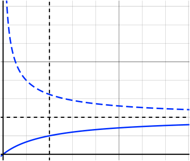
Figure 1: Simple form of the interpolating functions $\mu(a)$ (63), solid; and $\nu(h)$ (64), dashed. The scale $a_{0}$ is indicated by the vertical dashed line. The horizontal dashed line indicates 1 on the ordinate.

Appendix B A Mass + Quadrupole System

In spherical-polar coordinates $(r,\theta,\varphi)$, consider the potential

$$\psi(r,\theta)=-\frac{G\,M}{r}-\epsilon\frac{G\,M\,d^{2}}{r^{3}}\left(\frac{3}{2}\,\cos^{2}\theta-\frac{1}{2}\right),$$ (69)

where $\epsilon=\pm 1$. This potential describes a mass + a quadrupole system. It is straightforward to find ${\bm{h}}=-{\bm{\nabla}}\psi$, and then using ${\bm{g}}={\bm{h}}\,\nu(h)$ to find ${\bm{g}}$.

$${\bm{h}} =h_{r}\,\hat{{\bm{e}}}_{r}+h_{\theta}\,\hat{{\bm{e}}}_{\theta}$$ (70)

$$-\frac{h_{r}}{G\,M} =\frac{1}{r^{2}}+\frac{\epsilon\,d^{2}}{r^{4}}\cdot\tfrac{3}{2}(3\,\cos^{2}\theta-1)$$ (71)

$$-\frac{h_{\theta}}{G\,M} =\frac{\epsilon\,d^{2}}{r^{4}}\frac{3}{2}\,\sin(2\,\theta),$$ (72)

$$\frac{h^{2}}{(G\,M)^{2}} =\frac{1}{r^{4}}+\epsilon\,\frac{d^{2}}{r^{6}}(3\,\cos^{2}\theta-1)+{\cal O}\left(\frac{1}{r^{8}}\right)$$ (73)

Using either the simple or the standard form of the interpolating function, we get

$$\frac{\nu^{\prime}(h)}{h}\simeq\frac{1}{2}\,\sqrt{\frac{a_{0}}{(G\,M)^{5}}}\,r^{5},\qquad r\gg\sqrt{\frac{G\,M}{a_{0}}}=2\,b.$$ (74)

Now, using

$$\frac{h_{r}}{r} =-\frac{G\,M}{r^{3}}+{\cal O}\left(\frac{1}{r^{5}}\right),$$ (75)

$$\frac{\partial h^{2}}{\partial\theta} =\epsilon\,\frac{G^{2}\,M^{2}\,d^{2}}{r^{6}}\,3\,\sin(2\,\theta)+{\cal O}\left(\frac{1}{r^{8}}\right),$$ (76)

$$\frac{\partial h^{2}}{\partial r} =-\frac{G^{2}\,M^{2}}{r^{5}}+{\cal O}\left(\frac{1}{r^{7}}\right),$$ (77)

we can find the leading term of ${\bm{\nabla}}\times{\bm{g}}$.

$${\bm{\nabla}}\times{\bm{g}} =-{\bm{h}}\times{\bm{\nabla}}\nu(h)$$ (78)

$$=-\frac{\nu^{\prime}(h)}{2\,h}{\bm{h}}\times{\bm{\nabla}}h^{2}$$ (79)

$$=-\frac{\nu^{\prime}(h)}{2\,h}\left(\frac{h_{r}}{r}\frac{\partial h^{2}}{\partial\theta}-h_{\theta}\,\frac{\partial h^{2}}{\partial r}\right)\hat{{\bm{e}}}_{\varphi}$$ (80)

$$=-\frac{3}{4}\epsilon\sqrt{G\,M\,a_{0}}\cdot\frac{d^{2}}{r^{4}}\,\sin(2\,\theta)\,\hat{{\bm{e}}}_{\varphi}+{\cal O}\left(\frac{1}{r^{6}}\right).$$ (81)

Using the values given by Sofue [2017], we consider the following mass distribution for the Milky Way (excluding the halo):

1. A central black hole of mass $M_{\text{bh}}=3.6\times 10^{6}\,M_{\odot}$.

2. A spherical bulge of mass $M_{\text{b}}=9.2\times 10^{9}\,M_{\odot}$.

3. A disk of mass $M_{\text{D}}=4.0\times 10^{10}\,M_{\odot}$ with exponential density of length scale $a_{\text{D}}=5.0\,{\rm kpc}$.

From these figures we get

$$M =4.9\times 10^{10}\,M_{\odot},$$ (82)

$$\epsilon\,M\,d^{2} =-5\,M_{\text{D}}\,a_{\text{D}}^{2}=-5.0\times 10^{12}\,M_{\odot}\,{\rm kpc}^{2},$$ (83)

$$d =10\,{\rm kpc}.$$ (84)

acknowledgements

We would like to thank A.-H. Fatollahi for his valuable comments, which motivated the early version of this article. This work was partially supported by Alzahra University’s research council, and partly by Nazarbayev University.

References

- Alzain [2017] Alzain, M. (2017), J. Astrophys. Astron. 38 (4), 59.