Exact statistical mechanics of the Ising model on networks
Abstract
The Ising model is an equilibrium stochastic process used as a model in several branches of science including magnetic materials Ising:1925 , geophysics MaNJP:2019 , neuroscience SchneidmanNature:2006 , sociology StaufferAJP:2008 and finance Bornholdt:2001 . Real systems of interest have finite size and a fixed coupling matrix exhibiting quenched disorder. Exact methods for the Ising model, however, employ infinite size limits, translational symmetries of lattices and the Cayley tree BaxterBook:1989 , or annealed structures as ensembles of networks DorogovtsevPRE:2002 . Here we show how the Ising partition function can be evaluated exactly by exploiting small tree-width. This structural property is exhibited by a large set of networks KlemmJPC:2020 , both empirical and model generated.
A network is given by a finite node set and bond set . Figure 1(d) is an example of a small social network. The Hamiltonion assigns each spin configuration an energy
| (1) |
For the macrocanonical ensemble at temperature , our goal is to numerically evaluate the partition function
| (2) | ||||
| (3) |
The most naive approach directly performs the sum over all spin configurations. Efficiency is gained by summing over spin variables in an order chosen to suit the given network. Starting from a set of factors, each dependent on exactly two spin variables as in expression (3), the step-wise summation proceeds as follows. Let be the next node in the given order; multiply (expand) all factors dependent on , thus obtaining a single -dependent factor ; perform the summation over ; repeat until summation over all spin variables is done.
How do we choose an order of nodes that reduces computational cost? Crucially, part (3) of the computation generates a function depending at least on the neighbouring spin variables of node not yet summed over. Storing as a table of function values, this will use in time and memory for dependent on spin variables. If the network is a tree, the nodes are optimally ordered by descending distance from the root, such as node ordering in the tree shown in Figure 1(a). This ensures that the multiplication before each summation generates factors dependent on at most two spin variables.
The exact and fast computation on trees forms the basis for approximative methods for general networks. In belief propagation MezardBook:2009 , bits of information (so-called belief values) are passed along the bonds of the network. At each node , the incoming information is compiled assuming neighbours of being conditionally independent given spin . This approach is exact when the network is a tree. It still produces acceptable approximations when the network is locally tree-like DorogovtsevRMP:2008 so the length of cycles exceeds the expected correlation length of the process, at least in the limit of large system size DemboAAP:2010 . Most real networks, however, contain a large amount of short cycles due to their cliquishness Watts:1998 and modularity NewmanPNAS:2006 . Belief propagation has been been generalized to account for short cycles at least partially YedidiaNIPS:2000 ; RadicchiPRE:2016 ; Cantwell:2019 ; Kirkley:2021 .
In the present approach, we consider a different notion of tree-like structure for which exact rather than approximate computation is feasible. For integer , a -tree Bodlaender:2010 is obtained by iteratively adding a node and bonds from to each node in a -clique. Growth starts from a -clique network as initial condition. Since a -clique is a single node, a -tree is just a tree. A -clique is two nodes with a bond . A -tree is thus grown by choosing a bond in an existing -tree and joining nodes into a triangle with a newly added node . Equivalently, a -tree is obtained by augmenting a tree with a bond from each child node to the parent’s parent as shown in Figure 1(b). Using the same node ordering as for the underlying tree, the exact computation of the partition function is straight-forward, now involving factors depending on 3 spin variables at most. Figure 1(c) sketches an example of the computation.
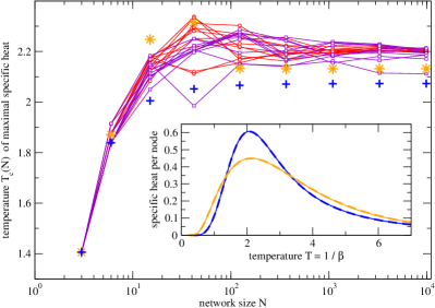
2-trees have been used as models of scale free-networks, including the sequential and parallel growth rules by Dorogovtsev et al. DorogovtsevPRE:2001 ; DorogovtsevPRE:2002b and the model by Klemm and Eguíluz KlemmPRE:2002a , see Methods. Figure 2 shows the critical Ising temperature , i.e. the value of maximizing the specific heat, for artificial 2-trees with sizes up to nodes. The plots suggest that remains bounded for growing , while is found for other growing and uncorrelated scale-free networks DorogovtsevRMP:2008 .
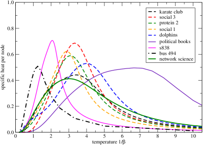
Empirical networks, though not being -trees, may be represented as partial -trees, often for KlemmJPC:2020 , by keeping only a subset of bonds in a -tree. Then there is an ordering of the nodes for which the calculation of the partition function involves factors depending on at most spin variables. The social network of Figure 1(d) is redrawn as a partial -tree structure with in Figure 1(e). Similarly, the 494 bus power system DavisACM:2011 , recently considered as a test network for loopy belief propagation Kirkley:2021 , is found to be a partial -tree, using the method from ref. KlemmJPC:2020 . For these two and further empirical networks, we calculate the exact specific heat of the Ising model at varying temperature, see Figure 3. For each choice of network and parameter , the calculation takes less than one second on a single processor core of a standard portable computer.
The present exact method is not restricted to the Ising model with all equal bonds but is equally efficient with any real-valued coupling strengths. These enter only in the initial factors of the computation. In spin glass models BinderRMP:1986 with frustrated Hamiltonians, ground state energies and freezing temperatures may be analyzed. We see potential to generalize the method to processes beyond the Ising model, such as bond and site percolation on networks RadicchiPRE:2015 .
Methods and Materials
Exact algorithm for the Ising partition function.
The algorithm takes as inputs a network given by a node set and bond set , a value of inverse temperature , and an ordering of . Operations take place on a collection of functions, called factors. Each factor has as its arguments one or several spin variables. Function values are real numbers. A factor can be implemented as a table or multidimensional array. Initially for each bond of the network, one factor with arguments and function values is contained in , cf. Equation (3). is computed in a loop with index running from to . For each , the following four operations are performed. (I) form the product of all factors in that depend on spin ; (II) remove these factors from ; (III) obtain by summing over in . (IV) include in . Upon completion of the loop, contains a single factor being a single number , the result of the computation.
Derivatives of .
The specific heat
| (4) | ||||
| (5) |
involves the first and second derivatives of , using . The exact values of these derivatives are computed within the same procedure as itself. For the first derivative, a function is generated initially for each bond . When forming the product of factors and in step (I) of the algorithm’s loop, the derivative is obtained as
| (6) |
for each configuration of spins these functions depend on. Likewise the second derivative of the same product is
| (7) | ||||
We initialize for each bond .
Models of growing 2-trees.
In all models, the initial condition is a network consisting of a single edge between two nodes. In the deterministic growth model by Dorogovtsev et al. DorogovtsevPRE:2002b , the network of generation is obtained by adding a node and forming a triangle simultaneously for each bond present at generation . The stochastic version of the model DorogovtsevPRE:2001 performs this node addition and triangle formation for one randomly selected bond in each microstep of growth. The growth and deactivation model by Klemm and Eguíluz KlemmPRE:2002a assigns each node a binary state as being active or inactive. In the initial condition, the two nodes present are active. At each step of growth, a new node forms a bond with each of the active nodes; is set active itself; out of the then three active nodes, one node is chosen randomly and deactivated. The probability of choosing a node for deactivation is proportional to , the inverse of the degree. If, instead, the oldest active node is deactivated in each step, a one-dimensional lattice with coordination number and open boundaries is obtained.
Elimination orders.
As empirical networks, we consider the karate club Zachary:1977 ; social 3, protein 2, social 1 Milo:2004 ; dolphins Lusseau:2003 , political books Krebs:2004 ; s 838 Milo:2002 ; network science Newman:2006 . For these networks (among others), suitable node orderings have been found by simulated annealing KlemmJPC:2020 , cf. the supplement of that article. For the 494 bus power system DavisACM:2011 , recently considered as a test network for loopy belief propagation Kirkley:2021 , a node ordering of maximum width 10 is found with the method of ref. KlemmJPC:2020 for all cooling schedules considered, even without any temperature variation.
Acknowledgments
Funding from MINECO through the Ramón y Cajal program and through project SPASIMM, FIS2016-80067-P (AEI/FEDER, EU) is acknowledged.
References
- [1] Ernst Ising. Beitrag zur Theorie des Ferromagnetismus. Zeitschrift für Physik, 31(1):253–258, 1925.
- [2] Yi-Ping Ma, Ivan Sudakov, Courtenay Strong, and Kenneth M Golden. Ising model for melt ponds on arctic sea ice. New Journal of Physics, 21(6):063029, 2019.
- [3] Elad Schneidman, Michael J. Berry II, Ronen Segev, and William Bialek. Weak pairwise correlations imply strongly correlated network states in a neural population. Nature, 440:1007–1012, 2006.
- [4] D. Stauffer. Social applications of two-dimensional Ising models. American Journal of Physics, 76(4):470–473, 2008.
- [5] Stefan Bornholdt. Expectation bubbles in a spin model of markets: Intermittency from frustration across scales. International Journal of Modern Physics C, 12(05):667–674, 2001.
- [6] Rodney J. Baxter. Exactly Solved Models in Statistical Mechanics. Academic Press (London), 1989.
- [7] S. N. Dorogovtsev, A. V. Goltsev, and J. F. F. Mendes. Ising model on networks with an arbitrary distribution of connections. Phys. Rev. E, 66:016104, 2002.
- [8] Konstantin Klemm. Tree decompositions of real-world networks from simulated annealing. Journal of Physics: Complexity, 1(3):035003, 2020.
- [9] Marc Mezard and Andrea Montanari. Information, Physics, and Computation. Oxford University Press, Inc., USA, 2009.
- [10] S. N. Dorogovtsev, A. V. Goltsev, and J. F. F. Mendes. Critical phenomena in complex networks. Rev. Mod. Phys., 80:1275–1335, 2008.
- [11] Amir Dembo and Andrea Montanari. Ising models on locally tree-like graphs. The Annals of Applied Probability, 20(2):565 – 592, 2010.
- [12] Duncan J Watts and Steven H Strogatz. Collective dynamics of small-world networks. Nature, 393(6684):440–442, 1998.
- [13] M. E. J. Newman. Modularity and community structure in networks. Proceedings of the National Academy of Sciences, 103(23):8577–8582, 2006.
- [14] Jonathan S. Yedidia, William T. Freeman, and Yair Weiss. Generalized belief propagation. In Advances in Neural Information Processing Systems 13, NIPS’00, pages 668–674, Cambridge, MA, USA, 2000. MIT Press.
- [15] Filippo Radicchi and Claudio Castellano. Beyond the locally treelike approximation for percolation on real networks. Phys. Rev. E, 93:030302, 2016.
- [16] George T. Cantwell and M. E. J. Newman. Message passing on networks with loops. Proceedings of the National Academy of Sciences, 116(47):23398–23403, 2019.
- [17] Alec Kirkley, George T. Cantwell, and M. E. J. Newman. Belief propagation for networks with loops. Science Advances, 7(17), 2021.
- [18] Hans L. Bodlaender and Arie M.C.A. Koster. Treewidth computations i. upper bounds. Information and Computation, 208(3):259–275, 2010.
- [19] Konstantin Klemm and Víctor M. Eguíluz. Highly clustered scale-free networks. Phys. Rev. E, 65:036123, Feb 2002.
- [20] S. N. Dorogovtsev, J. F. F. Mendes, and A. N. Samukhin. Size-dependent degree distribution of a scale-free growing network. Phys. Rev. E, 63:062101, 2001.
- [21] S. N. Dorogovtsev, A. V. Goltsev, and J. F. F. Mendes. Pseudofractal scale-free web. Phys. Rev. E, 65:066122, 2002.
- [22] Timothy A. Davis and Yifan Hu. The university of florida sparse matrix collection. ACM Trans. Math. Softw., 38(1), 2011.
- [23] K. Binder and A. P. Young. Spin glasses: Experimental facts, theoretical concepts, and open questions. Rev. Mod. Phys., 58:801–976, 1986.
- [24] Filippo Radicchi. Predicting percolation thresholds in networks. Phys. Rev. E, 91:010801, 2015.
- [25] Wayne W. Zachary. An information flow model for conflict and fission in small groups. Journal of Anthropological Research, 33(4):452–473, 1977.
- [26] Ron Milo, Shalev Itzkovitz, Nadav Kashtan, Reuven Levitt, Shai Shen-Orr, Inbal Ayzenshtat, Michal Sheffer, and Uri Alon. Superfamilies of evolved and designed networks. Science, 303(5663):1538–1542, 2004.
- [27] D Lusseau, K Schneider, O J Boisseau, P Haase, E Slooten, and S M Dawson. The bottlenose dolphin community of doubtful sound features a large proportion of long-lasting associations - can geographic isolation explain this unique trait? Behavioral Ecology and Sociobiology, 54:396–405, 2003.
- [28] Valdis Krebs, 2004. Unpublished, data posted online at http://www.orgnet.com/.
- [29] R. Milo, S. Shen-Orr, S. Itzkovitz, N. Kashtan, D. Chklovskii, and U. Alon. Network motifs: Simple building blocks of complex networks. Science, 298(5594):824–827, 2002.
- [30] M. E. J. Newman. Finding community structure in networks using the eigenvectors of matrices. Phys. Rev. E, 74:036104, 2006.