Numerical study of multiparticle production in $\phi^{4}$ theory:
comparison with analytic results

Abstract

We develop a numerical method to compute the probabilities of multiparticle production in weakly coupled scalar theories. Our technique is based on D.T. Son’s semiclassical method of singular solutions. Applying it to the process $1\to n$ in the unbroken four–dimensional $\lambda\phi^{4}$ theory, we reproduce the known results at ${1\ll n\ll\lambda^{-1}}$.

1 Introduction

It is well–known that perturbative expansion cannot be used to calculate the amplitudes with large numbers of external legs $n\gtrsim\lambda^{-1}$, where $\lambda$ is a small coupling constant [1, 2]. Indeed, resummation of perturbative series in $\lambda\phi^{4}$ theory [3, 4] indicates [5] that multiparticle production occurs with exponentially small probability at large $n$. Say, the inclusive probability of creating $n\gg 1$ particles from one off–shell particle equals

$${\cal P}_{1\to n}\left(E\right)\equiv\sum_{f}|\langle f;E,n|\hat{\cal S}\,\hat{\phi}(0)|0\rangle|^{2}\propto{\rm e}^{F_{1\to n}/\lambda},$$ (1)

where $\hat{\phi}(0)$ creates an off–shell in-state, $\hat{\cal S}$ is the S–matrix, the summation is performed over all final states with energy $E$ and multiplicity $n$, and we ignored inessential normalization factors and prefactors. Notably, the suppression exponent $F_{1\to n}<0$ in Eq. (1) depends on the combinations $\lambda n$ and $\lambda E$.

A considerable revival of the interest in multiparticle processes occurred recently [6, 7, 8, 9, 10, 11] when Ref. [12] suggested that, contrary to Eq. (1), the cross section of multiple Higgs boson production grows factorially at high energies. This ‘‘Higgsplosion’’ mechanism was subsequently criticised in [8, 13, 14, 15], so that now the situation is far from being settled. It is clear that further development of reliable methods for the calculation of multiparticle amplitudes is required.

Years ago, D.T. Son proposed [16] a general semiclassical framework to calculate the multiparticle probabilities at $\lambda n\sim O(1)$, see also [17, 18]. His technique is based on finding complex–valued singular solutions of classical field equations with appropriate boundary conditions. Despite being generic, this method was successfully applied only at $\lambda n\ll 1$ when semiclassical configurations can be deduced from simplified semi–analytic considerations.

In this Letter, we for the first time develop a complete numerical implementation of the D.T. Son’s semiclassical method of singular solutions. Our code computes the probability of the processes $1\to n$ in four–dimensional unbroken $\lambda\phi^{4}$ theory at arbitrary $\lambda n\sim 1$ and $\lambda E\sim O(m)$, where $m$ is the particle mass. As an initial step, we present here numerical results at $\lambda n\ll 1$ and demonstrate that they agree with predictions of the perturbation theory.

2 Semiclassical method for multiparticle production

In this Section, we review the method of [16] in application to a weakly coupled $(3+1)$–dimensional scalar field theory with the action,

$$S=\frac{1}{2\lambda}\int d^{4}x\left(\,-\phi\Box\phi-\phi^{2}-\phi^{4}/2\,\right)\;.$$ (2)

Here $\lambda\ll 1$ is the coupling constant that simultaneously plays the role of a semiclassical parameter and we work in units of the field mass $m=1$.

It is convenient to introduce the current $J$

$${\mathcal{P}}_{J}(E,n)=\sum_{f}|\langle f;n,E|\hat{\cal S}\,{\rm e}^{-J\hat{\phi}(0)/\lambda}|0\rangle|^{2},$$ (3)

so that the probability (1) equals

$${\mathcal{P}_{1\to n}=\lambda^{2}\,\lim\limits_{J\to 0}{\mathcal{P}}_{J}/J^{2}}\;.$$ (4)

In [16], the quantity (3) was represented as a path integral which is saturated at small $\lambda$ by a complex-valued saddle–point configuration $\phi(t,\,{\bm{x}})$. The saddle–point conditions for the latter include a classical field equation with the source term,

$$\Box\,\phi(x)+\phi(x)+\phi^{3}(x)=iJ\delta^{(4)}(x),$$ (5)

and certain boundary conditions. In particular, the semiclassical configuration should contain only the positive–frequency part in the infinite past,

$$\phi\to\int d^{3}{\bm{k}}\;{\rm e}^{-i{\bm{k}}{\bm{x}}+i\omega_{\bm{k}}t}\;a_{\bm{k}}\qquad\mbox{as}\qquad t\to-\infty\;,$$ (6)

where $a_{\bm{k}}$ are arbitrary and $\omega_{\bm{k}}=({\bm{k}}^{2}+1)^{1/2}$. At large positive times $t\to+\infty$ the solution is expected to linearize:

$$\phi\to\int\frac{d^{3}{\bm{k}}\;{\rm e}^{i{\bm{kx}}}}{(2\pi)^{3/2}\sqrt{2\omega_{\bm{k}}}}\left(\,f_{\bm{k}}{\rm e}^{-i\omega_{\bm{k}}t}+g_{-{\bm{k}}}^{*}{\rm e}^{i\omega_{\bm{k}}t}\,\right).$$ (7)

Saddle–point equations in this case relate the positive– and negative–frequency components of $\phi$,

$$f_{\bm{k}}={\rm e}^{-\theta+2\omega_{\bm{k}}T}\,g_{\bm{k}}\,,$$ (8)

where $T$ and $\theta$ have the sense of Lagrange multipliers appearing due to the fixation of energy $E$ and final–state multiplicity $n$. The latter quantities are given by the standard expressions,

$$\lambda E=\int d^{3}{\bm{k}}\,\omega_{\bm{k}}\,f_{\bm{k}}g_{\bm{k}}^{*}\;,\quad\lambda n=\int d^{3}{\bm{k}}\,f_{\bm{k}}g_{\bm{k}}^{*}\,.$$ (9)

In what follows we parametrise the solutions with the rescaled multiplicity $\lambda n$ and kinetic energy per particle ${\varepsilon\equiv E/n-1}$.

Once the semiclassical equations are solved, one finds the probability (1) by taking the limit

$${\cal P}_{1\to n}\approx\lim_{J\to 0}{\cal P}_{J}\approx\lim_{J\to 0}\mathrm{e}^{F_{J}/\lambda}\,,$$ (10)

where the prefactors are ignored and $F_{J}$ is the value of the functional

$$F_{J}/\lambda=2ET-n\theta-2{\rm Im}\,{S}-2J\,{\rm Re}\,\phi(0)/\lambda\;,$$ (11)

computed on the saddle-point solution $\phi(t,\,\bm{x})$.

It is important that the method of [16] involves a nontrivial assumption that the suppression exponent in Eq. (1) is universal, i.e. does not depend on the details of a few–particle initial state [19, 20, 21, 22]. In particular, the exponent is not sensitive to the choice of the source term in Eq. (3). However, in any case, the semiclassical solutions become singular at $t=0$ in the limit $J\to 0$, since their energies are equal to zero and $E$ at $t<0$ and $t>0$, respectively — see Eqs. (6), (9), and [23].

In the previous studies [16, 24, 25] the semiclassical solutions were found analytically at small $\lambda n$ and $\varepsilon$. It was shown that the semiclassical exponent $F_{1\to n}$ agrees with the one–loop perturbative results of Refs. [4, 26] in that region.

3 Numerical results

Let us outline the numerical method for solving the boundary problem (5)–(9) at arbitrary $\lambda n$ and $\varepsilon$. We analytically continue the solution to the complex time contour in Fig.1.

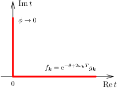
Рис. 1: Figure 1. Contour in complex time for the semiclassical boundary value problem (5)–(9).

Then Feynman initial condition (6) takes the form,

$$\phi(t,\,{\bm{x}})\to 0\qquad{\rm as}\qquad{\rm Im}\,t\to+\infty\,.$$ (12)

Besides, we regularize the source replacing

$$J\delta^{(4)}(x)\to j\,{\rm e}^{-{\bm{x}}^{2}/2\sigma^{2}}\delta(t)\,,$$ (13)

where $j$ and $\sigma$ will be sent to zero simultaneously. Next, we substitute the spherically–symmetric Ansatz $\phi=\phi(t,\,r)$ into the equation (5) and boundary conditions (6)–(8) and discretize the resulting system on the rectangular space–time lattice with sites $(t_{j},\,r_{k})$. The discrete problem is then solved using the Newton–Raphson method [27].

Changing $T$, $\theta$, $j$, and $\sigma$ in small steps, we find all regularised numerical solutions. The respective exponents $F_{J}(\varepsilon,\lambda n)$ are computed by performing integration in Eq. (11). An example of our semiclassical configuration $\phi(t,\,r)$ is given in Fig. 2.

Рис. 2: Figure 2. Semiclassical solution $\phi(t,\,r)$ with parameters ${\varepsilon\approx 1.35}$, ${\lambda n\approx 0.38}$, $j=0.3$, and ${\sigma\approx 0.1}$. Colour shows complex phase of $\phi$.

One observes a high and narrow peak at $t=r=0$ where the source is located. The solution becomes singular at this point in the limit $j,\sigma\to 0$. The outgoing waves represent the final–state particles emanating from the source.

The semiclassical expression (10) for the probability ${\cal P}_{1\to n}\approx\exp\{F_{1\to n}/\lambda\}$ includes the limit $j,\,\sigma\to 0$. Notably, the saddle–point configurations cannot be directly computed at $j=0$, as they are singular. We, therefore, perform a polynomial extrapolation of $F_{J}$ to $j=0$ keeping $j/\sigma=\mbox{const}$, cf. Eq. (4). The technical details of this procedure will be presented elsewhere [28].

To verify the numerical technique, we compare the multiparticle probability with the known perturbative results at small $\lambda n$. In this case, the semiclassical exponent $F_{1\to n}$ has the form [16],

$$F_{1\to n}=\lambda n\mathop{\rm ln}\nolimits\left(\frac{\lambda n}{16}\right)-\lambda n+\lambda nf(\varepsilon)+O(\lambda^{2}n^{2})\,,$$ (14)

where $\varepsilon\simeq O(1)$ and the function $f(\varepsilon)$ is unknown. The first three terms in Eq. (14) and, notably, $f(\varepsilon)$, can be extracted from tree–level diagrams. The latter calculation was performed numerically in [25] for arbitrary $\varepsilon$. It is worth noting that their result at $\varepsilon\leq 10$ almost saturates the simpler $O(4)$ bound of Ref. [29]. Below we use the latter for comparison.

Our results for $f(\varepsilon)$ are shown in Fig. 3 by circles with errorbars which represent inaccuracies of

Рис. 3: Figure 3. Numerical values of $f(\varepsilon)$ (circles with errorbars) compared with the tree–level results: $O(4)$–symmetric estimate of Refs. [29, 25] (solid line) and low–$\varepsilon$ expansion (15) (dashed).

the extrapolation $j\to 0$. These numerical data cover a finite energy range ${0.3\leq\varepsilon\leq 6}$. At smaller $\varepsilon$, the saddle–point solutions become nonrelativistic and fail to fit into the spacetime volume available for computations. At $\varepsilon\geq 6$ the solutions include higher–frequency waves which cannot be resolved.

Notably, the data points in Fig. 3 are consistent with the tree–level results previously obtained in the literature. They coincide with the $O(4)$ curve of Ref. [29] (solid line), as they should. Besides, both numerical graphs approach the low–$\varepsilon$ asymptotics of $f(\varepsilon)$,

$$f=\frac{3}{2}\mathop{\rm ln}\nolimits{\frac{\varepsilon}{3\pi}}+\frac{3}{2}-\frac{17}{12}\,\varepsilon\\ +\frac{1327-96\pi^{2}}{432}\,\varepsilon^{2}+O(\varepsilon^{3})\,,$$ (15)

that was evaluated analytically in [24].

4 Conclusions

We developed a numerical method to compute semiclassically the probabilities of $n$–particle production in scalar theories in the regime $n\to\infty$ and $\lambda n=$ fixed, where $\lambda$ is a small coupling constant. We illustrated the method by performing explicit calculations in a four–dimensional unbroken $\lambda\phi^{4}$ model. At $\lambda n\ll 1$ our numerical data for the probability agree with the tree–level results obtained previously in the literature. But notably, our technique is also applicable at ${\lambda n\sim O(1)}$.

This work is supported by the RFBR, grant № 20-32-90013. Numerical calculations were performed on the Computational cluster of the Theoretical Division of INR RAS.