The dynamic critical exponent $z$ for 2d and 3d Ising models from five-loop $\varepsilon$ expansion

Abstract

We calculate the dynamic critical exponent $z$ for 2d and 3d Ising universality classes by means of minimally subtracted five-loop $\varepsilon$ expansion obtained for the one-component model A. This breakthrough turns out to be possible through the successful adaptation of the Sector Decomposition technique to the problems of critical dynamics. The obtained fifth perturbative order accompanied by the use of advanced resummation techniques for asymptotic series allows us to find highly accurate numerical estimates of $z$: for two- and three-dimensional cases we obtain $\boldsymbol{2.14(2)}$ and $\boldsymbol{2.0235(8)}$ respectively. The numbers found are in good agreement with recent results obtained using different approaches.

1 Introduction

It is difficult to overstate the physical value of the concept of universality classes, proposed almost fifty years ago [1, 2]. Universality concerns a limited set of quantities including ratios of amplitudes and critical exponents [3, 4, 5, 6, 7]. The latter form a very canonical zoo. Static consideration of the critical behavior allows one to find all the exponents except one – the critical dynamic exponent $z$. In the case of completely dissipative relaxational dynamics of the order parameter, such an exponent characterizes the critical slowing down linking the correlation length $\xi$ and the typical time of fluctuations $\tau$ as: $\tau\propto\xi^{z}$. Both quantities – $\xi$ and $\tau$ – diverge at criticality that is caused by the strong fluctuations in the system approaching the critical point. Numerical values obtained within various theoretical and experimental approaches for this exponent can roughly be estimated as $z\simeq 2$. Determination of the exact numerical deviation of $z$ from the value of two plays a crucial role in the theory.

In order to theoretically investigate this phenomenon one can address the one-component model A of critical dynamics, which is in fact the simplest dynamic generalization of the scalar $\phi^{4}$ field theory (see Ref. [8]) sufficient to describe the critical slowing down for systems with the nonconserved order parameter and energy. The calculations of $z$ were carried out both using the Monte Carlo (MC) methods and different field theoretical (FT) approaches.

Lattice calculations can be performed in different ways. The system can be quenched from the state above or below the transition directly to the critical point. A comprehensive review of different nonequilibrium universality classes for lattice systems is given in Ref. [9]. For almost forty years, a large number of works have performed lattice calculations of $z$ for 2d and 3d Ising universality classes  [10, 11, 12, 13, 14, 15, 16, 17, 18, 19, 20, 21, 22, 23, 24, 25, 26, 27, 28, 28, 29, 30]. Let us only pay attention to the recent work [30], where $z$ was estimated as $2.0245(15)$ in three dimensions. This result was obtained by considering the so-called improved Blume-Capel model that allows authors to eliminate the leading corrections to scaling.

As for FT calculations, there is also a vast variety of results (see Ref. [31]). As is known, there are a number of different renormalization group (RG) approaches.

First, the RG analysis can be performed in fixed spatial dimensionality. The record-high result here is the four-loop calculations performed in Ref. [32]. For 2d and 3d Ising universality classes for $z$ the authors have obtained $2.0842(39)$ and $2.0237(55)$, respectively, by using the advanced resummation strategies in Ref. [33].

An alternative approach also applied to the problem is the so-called nonperturbative renormalization group (NPRG) [34, 35, 36]. In Ref. [34] the authors obtained the following estimates for two $2.16(1)$ and three $2.09(4)$ dimensions. A noticeably different number from the latter was found in Ref. [35]: $2.025$. The authors of Ref. [36], in turn, suggested a whole set of numerical estimates which correspond to application of different NPRG regulators (2d: $2.16$, $2.15$, $2.14$; 3d: $2.024$, $2.024$, $2.023$) and without them (2d: $2.28$; 3d: $2.032$).

The most canonical from the Wilson’s time RG formalism, within which the present work is carried out, is the $\varepsilon$ expansion approach. The idea to shift the critical dimension by a small quantity ($\text{d}=4-\varepsilon$) played a crucial role. The two-loop result was found almost fifty years ago in Ref. [37]. Ten years later, a three-loop contribution was added, which has been record-high for a long time [38]. The first attempt to calculate four-loop expansions was made in Ref. [39] with subsequent resummation in Ref. [40]. Only ten years later, however, the accuracy of four-loop calculations was notably improved [41] by means of a new diagram reduction technique. Thanks to this technique, we are able to calculate the five-loop contribution to $z$. In such a high order of perturbation theory (PT), the reduction in the number of diagrams turns out to be crucial: from $\boldsymbol{1025}$ to $\boldsymbol{201}$. The calculation of the diagrams themselves requires special attention in the case of critical dynamics. The main difference is that the form of the integrand corresponding to these diagrams is much complicated due to time dependence. For this purpose, we address the Sector Decomposition (SD) technique [42] as an effective method of accurate calculation of diagrams in the Feynman representation. It should be noted that initially SD was applied only to the static problems, where it has proven its efficiency. The authors of the present letter managed to adapt this method to critical dynamics diagrams [41]. The obtained five-loop expansion in combination with a novel resummation approach (we call it the free boundary condition method, which was developed on the basis of the boundary condition method suggested in Ref. [43]) makes it possible to extract highly accurate estimates for $z$, which allows excellent consistency with the numbers that were found within the recent MC [30] and NPRG [36] calculations. In this letter, we consider only some of the details of the calculation, giving special preference to the estimates of $z$.

Let us briefly cover the recent experimental results relevant to the problem. We note only that the experimental measurement of $z$ is fraught with enormous technical difficulties, which, so far, allows one to achieve only low numerical precision. Nevertheless, there is an extensive list of physical systems that are described by the one-component model A. For instance, in Ref. [44] the magnetoelectric dynamics in the multiferroic chiral antiferromagnet MnWO₄ was analyzed. The observation of critical slowing down of magnetoelectric fluctuations allowed the authors to make a conclusion about the validity of the theoretical description of this physical system within the model with overdamped magnetic 3d-Ising order parameter. The authors of other works [45, 46] studied the continuous phase transition of the AuAgZn₂ alloy by coherent x-ray scattering. Having quenched the alloy samples, they observed the motion of interfaces between ordered domains. Using the critical behaviour of the system, they also came to the conclusion that the critical dynamics of such a system corresponds to the one-component model A, although the number for dynamical critical exponent ($z=1.96(11)$) is in weak agreement with theoretical predictions. A result ($z\approx 2$) similar in accuracy was obtained in Ref. [47].

The structure of the letter is arranged as follows. In Section 2, we briefly cover the model description and some features of RG approach within critical dynamics. In Section 3, we apply different resummation techniques in order to extract proper numerical estimates for $z$. Finally, we come to a conclusion in Section 4.

2 Method

The action of the one-component model A is defined by a set of two scalar fields $\phi\equiv\{\psi,\,\psi^{\prime}\}$ and can be expressed as follows [7]:

$$S(\phi)=\lambda\psi^{\prime}\psi^{\prime}+\psi^{\prime}[-\partial_{t}\psi+\lambda(\partial^{2}\psi-m^{2}\psi-\frac{1}{3!}g\psi^{3})],$$ (1)

where $\lambda$ is the Onsager coefficient and $g$ is the coupling constant. The model A is multiplicatively renormalizable. In this work, we use the minimal subtraction renormalization scheme (MS). The details of the renormalization procedure can be found in Ref. [41]. As a result, we obtain RG series for various observables. The important point here is the resummation strategies which should be applied to these expansions. Quite often, in addition to the direct application of various resummation techniques, the numerical estimates can be improved by various hints regarding the critical exponent behavior. For example, in Ref. [48] alternative expansion for $z$ in terms of the new parameter $\varepsilon^{\prime}=d-1$ was obtained: $z=2+\varepsilon^{\prime}+\varepsilon^{\prime 2}/2+O(\varepsilon^{\prime 3})$. In addition, the authors resorted to information on the behavior of $z$ in $d=1,4$ spatial dimensionalities, as well as the behavior of the derivative. By combining this information and the canonical two-loop $\varepsilon$ expansion known at that time [37], they constructed the following Padé approximation:

$$z-2=\frac{(d-1)(4-d)^{2}}{c_{0}+c_{1}d+c_{2}d^{2}},$$ (2)

where the coefficients $c_{i}$ can be found from the condition of coincidence with the known $\varepsilon$ and $\varepsilon^{\prime}$ expansions. The same trick was done in Ref. [30] based on the known four-loop results [41].

In this letter, on the basis of the calculated five-loop contribution, we obtain numerical estimates for $z$ by means of the modified conformal mapping (CM) resummation technique that takes into account the strong coupling asymptotics. Padé approximations are found both directly for five-loop $\varepsilon$ expansion and with the help of the known two-loop $\varepsilon^{\prime}$ series.

3 Results

The five-loop $\varepsilon$ expansion of $z$ for the one-component model A reads:

$$z=2+0.013446\varepsilon^{2}+0.011037\varepsilon^{3}-0.0055791(4)\varepsilon^{4}+\boldsymbol{0.01774(31)}\varepsilon^{5}+O(\varepsilon^{6}).\,\,$$ (3)

The way of calculating the corresponding five-loop diagrams deserves a separate consideration; here we focus on extracting numerical estimates from the series (3).

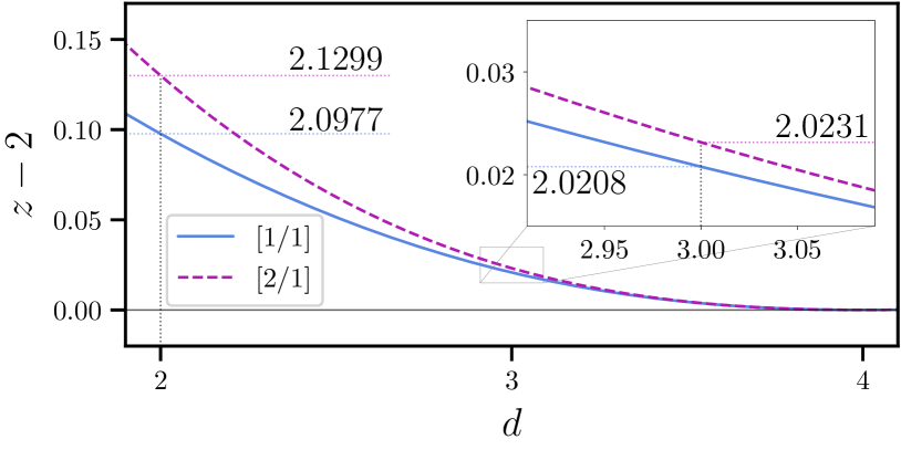
Figure 1: The dependence of Padé approximants $[1/1]$ and $[2/1]$ on spatial dimensionality. The approximations are constructed based on $\varepsilon$ expansion (3). In the figure, we highlight the physically interesting values of $z$ given by both approximants.

First, let us extract the desired numbers based on the Padé approximations directly for the series (3). The structure of the corresponding approximants reads:

$$z-2\approx(4-d)^{2}\dfrac{P^{(L)}(d)}{Q^{(M)}(d)}=[L/M],\qquad L+M=3\,,$$ (4)

where $P^{(L)}(d)$ and $Q^{(M)}(d)$ are polynomials in $d$ of order $L$ and $M$, respectively. Their coefficients are found from the condition that the truncated Taylor series of the given ratio $[L/M]$ (or specific Padé approximant) coincides with the original part of asymptotic expansion. Eliminating approximations spoiled by dangerous poles, we are left with only two of them. Here, by spoiled approximants we mean those approximations, which have in the denominator the roots located in the physical domain in terms of spatial dimensionality: $d\in[1,4]$. The behaviour of these approximations as well as the corresponding estimates of $z$ for 2d and 3d cases are presented in Fig. 1.

Taking into account two-loop $\varepsilon^{\prime}$ expansion [48] allows us to introduce two additional conditions on the coefficients for Padé approximations:

$$z-2\approx(4-d)^{2}(d-1)\dfrac{P^{(L)}(d)}{Q^{(M)}(d)}=[L/M],\quad L+M=5\,.$$ (5)

In order to demonstrate the convergence of estimates with increasing PT order, adhering to this resummation strategy, we depicted the trends on the upper (2d) and lower (3d) panels in Fig. 2. The corresponding five-loop estimates are $2.1772$ and $2.0251$, respectively. Despite a significant improvement in the numerical estimates, which is noticeable by their agreement with the results of other theoretical methods, these numbers still do not allow us to form a stable sample on the basis of which a final estimate could be proposed.

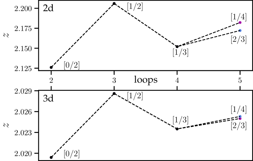
Figure 2: The behaviour of estimates for $z$ based on different Padé approximations (5) with regard to the number of loops. Except the five-loop case for each perturbation order only one approximant is not spoiled by poles.

A more consistent way of resummation an asymptotic series $z-2=\sum_{n}A_{n}\varepsilon^{n}$ is to consider the Borel resummation technique, which is applicable to expansions with factorially increasing coefficients: $A_{n}=C\,n!\,n^{b_{0}}(-a)^{n}(1+O(1/n))$, $n\to\infty$. For the one-component model A these parameters were calculated in Ref. [49]: $a=1/3$ and $b_{0}=7/2$. As a result of the so-called Borel transformation, one can obtain the Borel image $F(x)$:

$$\sum\limits_{n}A_{n}\varepsilon^{n}=\int\limits_{0}^{\infty}dt\,e^{-t}t^{b}\sum\limits_{n}B_{n}(\varepsilon t)^{n}=\int\limits_{0}^{\infty}dt\,e^{-t}t^{b}F(\varepsilon t)\,.\,\,$$ (6)

The analytical continuation of $F(x)$ has to be constructed, which is dictated by its finite convergence radius ($1/a$). One of the ways to obtain it is a conformal mapping of a particular form: $w(\varepsilon t)=(\sqrt{1+a\varepsilon t}-1)/(\sqrt{1+a\varepsilon t}+1)$. It transforms the real semiaxis into $[0,1)$ making the integration region within a circle of convergence. Thus, it results in the following rewritten expansion:

$$\int\limits_{0}^{\infty}dt\,e^{-t}\,t^{b}\,\left(\dfrac{\varepsilon t}{w(\varepsilon t)}\right)^{\lambda}\sum\limits_{n}B_{n}^{(w)}w^{n}\,,\quad b=b_{0}+\dfrac{3}{2},$$ (7)

where $B_{n}^{(w)}$ can be calculated by means of reexpanding $F(\varepsilon t)$ in terms of the new variable $w$. The introduced multiplier – $\left(\varepsilon t/w(\varepsilon t)\right)^{\lambda}$ – is responsible for taking into account the strong coupling asymptotics: $A(\varepsilon)\sim\varepsilon^{\lambda},\,\varepsilon\to\infty.$ As will be shown below, such manipulation also improves the convergence of estimates. However, the parameter of strong coupling asymptotics $\lambda$ for the model A is unknown. In Ref. [50], the authors suggested to use $\lambda$ as a fitting parameter to improve the convergence. The criterion of its selection is the rate of convergence of the resummed results with sequential considering the known orders. The corresponding behaviour of 3d $z$ estimates for different $\lambda$ is presented in Fig. 3. The observed tendency towards convergence of the results of calculations weakens with increasing order of PT.

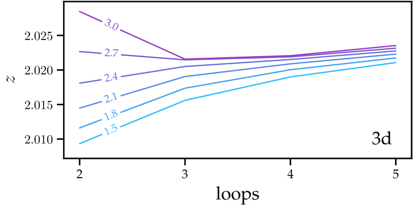
Figure 3: The behavior of estimates for critical exponent $z$ based on the order of PT for different values of $\lambda$.

The situation can further be improved by resorting to the technique used earlier for calculating static exponents in Ref. [43]. It was proposed to use the known values of critical exponents in other spatial dimensions. Unfortunately, for the dynamic critical exponent $z$ the exact value at any numerically helpful dimensions is unknown. However, we may use a trick according to which the value at a certain boundary point can be considered as a variable quantity determined only by the requirement of best convergence of the resummation procedure. The dependence of numerical estimates of $z$ in a three-dimensional case when the boundary value at two dimensions – $z_{b}$ – is assumed to be $2.13$ is presented in Fig. 4. As can be seen from the figure, the convergence has been noticeably improved in comparison with the case in Fig. 3. As the optimal values of $\lambda$ and $z_{b}$, one should choose those that provide the best convergence to a given limit value based on a smaller number of terms of PT under consideration. This, in turn, corresponds to the fastest decrease in the slope of the straight line with an increasing number of loops. In order to formalize the convergence criterion, we write down the equation of the straight line passing through the points of four- ($z^{(4)}$) and five-loop ($z^{(5)}$) approximations as follows:

$$z(l)=a(\lambda)(l-5)+b(\lambda)\,,$$ (8)

where $l$ is the number of loops, $a(\lambda)=z^{(5)}-z^{(4)}$ and $b(\lambda)=z^{(5)}$. It is natural to demand the least sensitivity of the slope of the straight line $z(l)$ to the $\lambda$ variation that, in turn, compels the derivatives $\partial_{\lambda}a$, $\partial_{\lambda}b$, and $\partial_{\lambda}^{2}b$ to take their minimum values. Therefore, as a criterion of convergence, one can choose the requirement of the minimum value of the following quantity:

$$Q=\sqrt{\left(\partial_{\lambda}a\right)^{2}+\left(\partial_{\lambda}b\right)^{2}+\left(\partial_{\lambda}^{2}b\right)^{2}}.$$ (9)

We demonstrate the minimal value on the projection of the $Q(\lambda,z_{b})$-surface as an inset in Fig. 4, which corresponds to the best convergence of estimates for the 3d case when the boundary point is $d=2$ and the calculation point is $d=3$. The choice of optimal parameters is not critical within the moderate range for $\varepsilon$. To obtain the final estimates, averaging is carried out over both the boundary and calculation points. Our five-loop estimates obtained by means of this resummation technique are $2.13(4)$ and $2.023(2)$ for two and three dimensions, respectively. A comparison of the results obtained by means of the free boundary condition and without it shows that this modification of the CM resummation technique gives better agreement with the estimates of $z$ obtained in recent works [30, 36, 35].

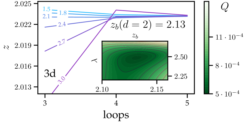
Figure 4: The behaviour of numerical estimates for critical exponent $z$ based on the order of PT for different values of $\lambda$ in the case of taking into account the boundary condition: $z_{2d}=2.13$.

In addition, we can address the way of numerical estimation of $z$ suggested in Ref. [37] via resummation of auxiliary quantity $c$, which is related to $z$ by $z=2+c\eta$, where $\eta$ is the static Fisher exponent. Taking into account the $\varepsilon$ expansion for $\eta$ from Ref. [51, 52] and the series (3) for $c$, we obtain:

$$c=0.72609(1-0.18845\varepsilon+0.22503(3)\varepsilon^{2}-0.379(23)\varepsilon^{3})+O(\varepsilon^{4}).\,\,\,\,$$ (10)

Bearing in mind the fact that the coefficients of the series (10) are small, it is hoped that the difficulties of analysis of the series manifest themselves only for the exponent $\eta$. In order to estimate $c$ from expansion (10), we find four- and five-loop Padé approximants: $[1/1]$, $[2/1]$ and $[1/2]$. Averaging the obtained estimates for $c$ over two approximations and using the exact values $\eta=1/4$ for $d=2$ and the most accurate $\eta=0.0362978(20)$ for $d=3$ [53], for the exponent $z$ we obtain $2.1512$ and $2.0236$ respectively.

Finally, we apply the KP17 method [52] which gives the most reliable results for $\phi^{4}$ [52] and $\phi^{3}$ [54, 55] models. This resummation technique includes three resummation parameters: $b$, $\lambda$, and $q$, where $b$ and $\lambda$ enter the expression (7). The latter is responsible for the so-called homographic transformation, which allows one to take into account the potentially possible pole singularities of the $\varepsilon$ expansion. The selection strategy for these parameters is based on the their varying over a wide ranges in order to find the area of greatest stability of analyzed quantity. Here we have an additional source of error due to uncertainty of the numerical calculation of 4-th and 5-th terms, thus we add additional term related to this uncertainty. The corresponding results were added to Table 1.

Table 1: Numerical estimates of $z$ obtained by means of different resummation strategies.

Loops	Dim.	Simple	Padé via	Via coup.	Free	KP17
		Padé	$\varepsilon^{\prime}$ exp.	const. c	b.c.	Ref. [52]
4	2d	2.098	2.150	2.161	2.10(16)	2.11(11)
	3d	2.021	2.024	2.024	2.021(5)	2.023(4)
5	2d	2.130	2.177	2.151	2.13(4)	2.15(3)
	3d	2.023	2.025	2.0236	2.023(2)	2.0239(14)

4 Conclusions

As a final estimate for the exponent $z$, we choose the weighted average calculated on the basis of all five-loop numbers from Table 1. The validity of this step is described in Ref. [54]. This tactic allows us to take into account an error bar of a particular sample element. Thus, for two- and three-dimensional cases we have $\boldsymbol{2.14(2)}$ and $\boldsymbol{2.0236(8)}$, respectively. These numbers are found in good agreement with the recently found results (2d: $2.1667(5)$ (MC [26]), $\sim 2.15$ (NPRG [36])) and (3d: $\sim 2.024$ (NPRG [36]), $2.0245(15)$ (MC [30])) and can be considered as reliable ones. Special attention, however, should be paid to the improvement of the results obtained by the CM resummation method together with the used strategy for determining the optimal values of the strong coupling parameter $\lambda$ and the optimal value at the boundary point $z_{b}$ by the convergence criterion $Q$. The applied method of the free boundary condition has noticeably accelerated the convergence of the resummation procedure, which may indicate its effectiveness in being applied to other models, where exact values of the quantities of interest in different spatial dimensions are unknown. Also, taking into account the $\varepsilon^{\prime}=d-1$ expansion shows high efficiency in refining the results. This is especially pronounced when the four terms of the $\varepsilon$ expansion are taken into account, and additional information allows one to obtain a much more accurate value of $z$ compared to other methods. This is evidence in favor of using similar alternative expansions in the resummation procedure. Since the calculation of the six-loop coefficient of the $\varepsilon$ expansion for $z$ is a challenging computational problem, the results obtained may indicate the expediency of calculating the following orders in the $\varepsilon^{\prime}$ expansion.

References

- [1] M. Green, J. Sengers, Critical Phenomena: Proceedings of a Conference Held in Washington, D. C., April 1965, Forgotten Books, 2017.
- [2] M. Green, Critical phenomena: International School of Physics ”Enrico Fermi” (51st : 1970 : Varenna, Italy), Academic Press New York, 1971.
- [3] K. G. Wilson, J. Kogut, The renormalization group and the expansion, Phys. Rep. 12 (2) (1974) 75.
- [4] M. E. Fisher, The renormalization group in the theory of critical behavior, Rev. Mod. Phys. 46 (1974) 597.
- [5] J. Zinn-Justin, Quantum Field Theory and Critical Phenomena, Clarendon Press, Oxford, 1989, 1993, 2002.
- [6] A. Pelissetto, E. Vicari, Critical phenomena and renormalization-group theory, Phys. Rep. 368 (2002) 549.
- [7] A. N. Vasil’ev, Quantum field renormalization group in critical behavior theory and stochastic dynamics, Chapman & Hall/CRC, 2004, originally published in Russian in 1998 by St. Petersburg Institute of Nuclear Physics Press; translated by Patricia A. de Forcrand-Millard.
- [8] P. C. Hohenberg, B. I. Halperin, Theory of dynamic critical phenomena, Rev. Modern Phys. 49 (3) (1977) 435.
-
[9]
G. Ódor,
Universality
classes in nonequilibrium lattice systems, Rev. Mod. Phys. 76 (2004)
663–724.
doi:10.1103/RevModPhys.76.663.
URL https://link.aps.org/doi/10.1103/RevModPhys.76.663 -
[10]
S. Wansleben, D. P. Landau, Dynamical
critical exponent of the 3d ising model, J. Appl. Phys. 61 (8) (1987)
3968–3970.
doi:10.1063/1.338572.
URL https://doi.org/10.1063/1.338572 -
[11]
S. Wansleben, D. P. Landau,
Monte carlo
investigation of critical dynamics in the three-dimensional ising model,
Phys. Rev. B 43 (1991) 6006–6014.
doi:10.1103/PhysRevB.43.6006.
URL https://link.aps.org/doi/10.1103/PhysRevB.43.6006 -
[12]
C. Münkel, D. W. Heermann, J. Adler, M. Gofman, D. Stauffer,
The dynamical critical
exponent of the two-, three- and five-dimensional kinetic ising model, Phys.
A 193 (3-4) (1993) 540–552.
doi:10.1016/0378-4371(93)90490-u.
URL https://doi.org/10.1016/0378-4371(93)90490-u -
[13]
N. Ito,
Non-equilibrium
critical relaxation of the three-dimensional ising model, Phys. A 192 (4)
(1993) 604–616.
doi:https://doi.org/10.1016/0378-4371(93)90111-G.
URL https://www.sciencedirect.com/science/article/pii/037843719390111G - [14] N. Ito, Non-equilibrium relaxation and interface energy of the ising model, Phys. A 196 (4) (1993) 591–614.
- [15] P. Grassberger, Damage spreading and critical exponents for “model a” ising dynamics, Phys. A 214 (4) (1995) 547–559.
-
[16]
Z. B. Li, L. Schülke, B. Zheng,
Dynamic monte
carlo measurement of critical exponents, Phys. Rev. Lett. 74 (1995)
3396–3398.
doi:10.1103/PhysRevLett.74.3396.
URL https://link.aps.org/doi/10.1103/PhysRevLett.74.3396 - [17] U. Gropengiesser, Damage spreading and critical exponents for ‘model a’ising dynamics, Phys. A 215 (3) (1995) 308–310.
-
[18]
M. P. Nightingale, H. W. J. Blöte,
Dynamic exponent
of the two-dimensional ising model and monte carlo computation of the
subdominant eigenvalue of the stochastic matrix, Phys. Rev. Lett. 76 (1996)
4548–4551.
doi:10.1103/PhysRevLett.76.4548.
URL https://link.aps.org/doi/10.1103/PhysRevLett.76.4548 - [19] D. Stauffer, et al., Flipping of magnetization in ising models at tc, Int. J. Mod. Phys. C 7 (5) (1996) 753–758.
-
[20]
M. Silvério Soares, J. Kamphorst Leal da Silva, F. C. SáBarreto,
Numerical method to
evaluate the dynamical critical exponent, Phys. Rev. B 55 (1997) 1021–1024.
doi:10.1103/PhysRevB.55.1021.
URL https://link.aps.org/doi/10.1103/PhysRevB.55.1021 -
[21]
F.-G. Wang, C.-K. Hu,
Universality in
dynamic critical phenomena, Phys. Rev. E 56 (1997) 2310–2313.
doi:10.1103/PhysRevE.56.2310.
URL https://link.aps.org/doi/10.1103/PhysRevE.56.2310 -
[22]
J.-S. Wang, C. K. Gan,
Nonequilibrium
relaxation of the two-dimensional ising model: Series-expansion and monte
carlo studies, Phys. Rev. E 57 (1998) 6548–6554.
doi:10.1103/PhysRevE.57.6548.
URL https://link.aps.org/doi/10.1103/PhysRevE.57.6548 - [23] A. Jaster, J. Mainville, L. Schülke, B. Zheng, Short-time critical dynamics of the three-dimensional ising model, J. Phys. A: Math. Gen. 32 (8) (1999) 1395.
- [24] C. Godreche, J. Luck, Response of non-equilibrium systems at criticality: ferromagnetic models in dimension two and above, J. Phys. A: Math. Gen. 33 (50) (2000) 9141.
-
[25]
N. Ito, K. Hukushima, K. Ogawa, Y. Ozeki,
Nonequilibrium relaxation of
fluctuations of physical quantities, J. Phys. Soc. Japan 69 (7) (2000)
1931–1934.
doi:10.1143/JPSJ.69.1931.
URL https://doi.org/10.1143/JPSJ.69.1931 -
[26]
M. P. Nightingale, H. W. J. Blöte,
Monte carlo
computation of correlation times of independent relaxation modes at
criticality, Phys. Rev. B 62 (2000) 1089–1101.
doi:10.1103/PhysRevB.62.1089.
URL https://link.aps.org/doi/10.1103/PhysRevB.62.1089 -
[27]
X. Lei, J. Zheng, X. Zhao,
Monte carlo simulations for
two-dimensional ising system far from equilibrium, Chinese Sci. Bull. 52 (3)
(2007) 307–312.
doi:10.1007/s11434-007-0060-0.
URL https://doi.org/10.1007/s11434-007-0060-0 - [28] Y. Murase, N. Ito, Dynamic critical exponents of three-dimensional ising models and two-dimensional three-states potts models, J. Phys. Soc. Japan 77 (1) (2008) 014002.
-
[29]
M. Collura,
Off-equilibrium
relaxational dynamics with an improved ising hamiltonian, J. Stat. Mech.
Theory Exp. 2010 (12) (2010) P12036.
doi:10.1088/1742-5468/2010/12/p12036.
URL https://doi.org/10.1088/1742-5468/2010/12/p12036 -
[30]
M. Hasenbusch,
Dynamic critical
exponent of the three-dimensional ising universality class: Monte carlo
simulations of the improved blume-capel model, Phys. Rev. E 101 (2020)
022126.
doi:10.1103/PhysRevE.101.022126.
URL https://link.aps.org/doi/10.1103/PhysRevE.101.022126 - [31] R. Folk, G. Moser, Critical dynamics: a field-theoretical approach, J. Phys. A: Math. Gen. 39 (2006) R207.
- [32] V. V. Prudnikov, A. V. Ivanov, A. A. Fedorenko, Critical dynamics of spin systems in the four-loop approximation, J. Exp. Theor. Phys. 66 (1997) 835.
- [33] A. Krinitsyn, V. V. Prudnikov, P. V. Prudnikov, Calculations of the dynamical critical exponent using the asymptotic series summation method, Theor. Math. Phys. 147 (1) (2006) 561–575.
-
[34]
L. Canet, H. Chaté,
A non-perturbative
approach to critical dynamics, J. Phys. A: Math. Theor. 40 (9) (2007)
1937–1949.
doi:10.1088/1751-8113/40/9/002.
URL https://doi.org/10.1088%2F1751-8113%2F40%2F9%2F002 - [35] D. Mesterházy, J. H. Stockemer, Y. Tanizaki, From quantum to classical dynamics: The relativistic model in the framework of the real-time functional renormalization group, Phys. Rev. D 92 (2015) 076001.
-
[36]
C. Duclut, B. Delamotte,
Frequency
regulators for the nonperturbative renormalization group: A general study and
the model a as a benchmark, Phys. Rev. E 95 (2017) 012107.
doi:10.1103/PhysRevE.95.012107.
URL https://link.aps.org/doi/10.1103/PhysRevE.95.012107 -
[37]
B. I. Halperin, P. C. Hohenberg, S.-k. Ma,
Calculation of
dynamic critical properties using wilson’s expansion methods, Phys. Rev.
Lett. 29 (1972) 1548–1551.
doi:10.1103/PhysRevLett.29.1548.
URL https://link.aps.org/doi/10.1103/PhysRevLett.29.1548 -
[38]
N. V. Antonov, A. N. Vasil'ev,
Critical dynamics as a field
theory, Theoret. Math. Phys. 60 (1) (1984) 671–679.
doi:10.1007/bf01018251.
URL https://doi.org/10.1007/bf01018251 - [39] L. T. Adzhemyan, S. Novikov, L. Sladkoff, Calculation of dynamical exponent in model a of critical dynamics to order 4, Vestnik SPbSU Phys. Chem. 4 (4) (2008) 110.
- [40] M. Y. Nalimov, V. A. Sergeev, L. Sladkoff, Borel resummation of the -expansion of the dynamical exponent z in model a of the 4 (o (n)) theory, Theoret Math. Phys. 159 (1) (2009) 499–508.
- [41] L. T. Adzhemyan, E. Ivanova, M. Kompaniets, S. Y. Vorobyeva, Diagram reduction in problem of critical dynamics of ferromagnets: 4-loop approximation, J. Phys. A: Math. Theor. 51 (15) (2018) 155003.
-
[42]
T. Binoth, G. Heinrich,
Numerical
evaluation of multi-loop integrals by sector decomposition, Nuclear Physics
B 680 (1) (2004) 375–388.
doi:https://doi.org/10.1016/j.nuclphysb.2003.12.023.
URL https://www.sciencedirect.com/science/article/pii/S0550321303010800 - [43] R. Guida, J. Zinn-Justin, Critical exponents of the n-vector model, J. Phys. A: Math. Gen. 31 (40) (1998) 8103.
- [44] D. Niermann, C. Grams, P. Becker, L. Bohatỳ, H. Schenck, J. Hemberger, Critical slowing down near the multiferroic phase transition in mnwo 4, Phys. Rev. Lett. 114 (3) (2015) 037204.
- [45] F. Livet, M. Fèvre, G. Beutier, M. Sutton, Ordering fluctuation dynamics in auagzn 2, Phys. Rev. B 92 (9) (2015) 094102.
- [46] F. Livet, M. Fèvre, G. Beutier, F. Zontone, Y. Chushkin, M. Sutton, Measuring the dynamical critical exponent of an ordering alloy using x-ray photon correlation spectroscopy, Phys. Rev. B 98 (1) (2018) 014202.
-
[47]
F. Livet, F. m. c. Bley, J.-P. Simon, R. Caudron, J. Mainville, M. Sutton,
D. Lebolloc’h,
Statics and
kinetics of the ordering transition in the alloy,
Phys. Rev. B 66 (2002) 134108.
doi:10.1103/PhysRevB.66.134108.
URL https://link.aps.org/doi/10.1103/PhysRevB.66.134108 -
[48]
R. Bausch, V. Dohm, H. K. Janssen, R. K. P. Zia,
Critical dynamics
of an interface in dimensions, Phys. Rev. Lett. 47
(1981) 1837–1840.
doi:10.1103/PhysRevLett.47.1837.
URL https://link.aps.org/doi/10.1103/PhysRevLett.47.1837 - [49] J. Honkonen, M. Komarova, M. Y. Nalimov, Large-order asymptotes for dynamic models near equilibrium, Nucl. Phys. B Proc. Suppl. 707 (3) (2005) 493–508.
-
[50]
M. Kompaniets, Prediction
of the higher-order terms based on borel resummation with conformal mapping,
J. Phys. Conf. Ser. 762 (2016) 012075.
doi:10.1088/1742-6596/762/1/012075.
URL https://doi.org/10.1088/1742-6596/762/1/012075 -
[51]
D. Batkovich, K. Chetyrkin, M. Kompaniets,
Six
loop analytical calculation of the field anomalous dimension and the critical
exponent in o (n)-symmetric 4 model, Nucl. Phys. B 906
(2016) 147–167.
doi:https://doi.org/10.1016/j.nuclphysb.2016.03.009.
URL https://www.sciencedirect.com/science/article/pii/S0550321316000912 - [52] M. V. Kompaniets, E. Panzer, Minimally subtracted six-loop renormalization of o (n)-symmetric 4 theory and critical exponents, Phys. Rev. D 96 (3) (2017) 036016.
- [53] D. Simmons-Duffin, The lightcone bootstrap and the spectrum of the 3d ising cft, J. High Energy Phys. 03 (2017) 086.
-
[54]
M. Borinsky, J. A. Gracey, M. V. Kompaniets, O. Schnetz,
Five-loop
renormalization of theory with applications to the
lee-yang edge singularity and percolation theory, Phys. Rev. D 103 (2021)
116024.
doi:10.1103/PhysRevD.103.116024.
URL https://link.aps.org/doi/10.1103/PhysRevD.103.116024 -
[55]
M. Kompaniets, A. Pikelner,
Critical
exponents from five-loop scalar theory renormalization near six-dimensions,
Phys. Lett. B 817 (2021) 136331.
doi:https://doi.org/10.1016/j.physletb.2021.136331.
URL https://www.sciencedirect.com/science/article/pii/S0370269321002719