OMD: Orthogonal Malware Detection using Audio, Image, and Static Features

Abstract

With the growing number of malware and cyber attacks, there is a need for “orthogonal” cyber defense approaches, which are complementary to existing methods by detecting unique malware samples that are not predicted by other methods. In this paper, we propose a novel and orthogonal malware detection (OMD) approach to identify malware using a combination of audio descriptors, image similarity descriptors and other static/statistical features. First, we show how audio descriptors are effective in classifying malware families when the malware binaries are represented as audio signals. Then, we show that the predictions made on the audio descriptors are orthogonal to the predictions made on image similarity descriptors and other static features. Further, we develop a framework for error analysis and a metric to quantify how orthogonal a new feature set (or type) is with respect to other feature sets. This allows us to add new features and detection methods to our overall framework. Experimental results on malware datasets show that our approach provides a robust framework for orthogonal malware detection.

I Introduction

Despite increasing efforts in computer security, malware continues to be a large problem for everyone from private individuals to national governments. With the significant number of new malware being generated, it is difficult for traditional methods to keep up. Today’s commercial Antivirus defense mechanisms are based on scanning computers for suspicious activity. If such an activity is found, the suspected files are quarantined and the vulnerable system is patched with an update. In turn, the Antivirus software are also updated with new signatures to identify such activities in future. These scanning methods are based on a variety of techniques such as static analysis, dynamic analysis, and other heuristics based techniques, which are often slow to react to new attacks and threats. While this signatures battle front is being fought, it may be beneficial for the defender to open several more cyber battle fronts to make it more expensive for an adversary to develop successful/undetected exploits. A new cyber battle front implies that it employs new detection vectors which are “orthogonal” (independent) to the already existing malware detection methods, i.e., a new detection method correctly identifies malware that are not detected by existing methods. In this way, orthogonal detections can help reduce the large number of malware and exploits targeted towards military networked computing systems.

Figure 1: Overall framework of OMD - A malware detection system where multiple input feature types (static, statistical, image, audio) are passed through Machine Learning (ML) classifiers. The predictions from these classifiers are then checked to see if the features are orthogonal.

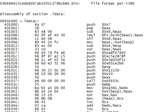
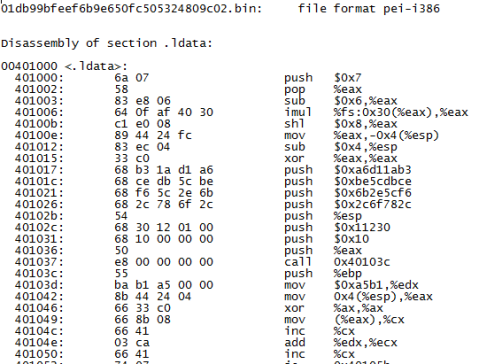
Figure 2: Disassembly of two variants from Alueron family where most of the instructions between the two variants are same.

In prior work, we have demonstrated effective automated malware classification by recasting software binaries as signals/images and exploiting computer vision techniques  [1, 2]. In this paper, we extend this approach by representing malware binaries as audio signals and computing audio descriptors to classify malware. Then, we show how the predictions made on audio descriptors are orthogonal to predictions made on other methods like image similarity features and static analysis features. Since malware authors are usually familiar with standard detection methods and produce new malware that evades these techniques, the hope is that these orthogonal methods raise the difficulty factor and cost for successfully developing and deploying new malware. We demonstrate our orthogonal malware detection (OMD) framework on standard static features based on code disassembly, n-grams, as well as signal processing based features such as image and audio descriptors. We focus on static and signal processing methods as a proof of concept, but our framework can be easily extended to other methods like dynamic analysis as long as these methods are orthogonal. The overall framework of our proposed OMD approach is shown in Figure 1. The main contributions of this paper are:

• We first show how the similarity of malware variants when represented as audio signals can be leveraged for identifying malware families. We then perform a thorough investigation of audio descriptors for malware classification and detection.

• We also show how the predictions based on audio descriptors are orthogonal to predictions based on other static and statistical features.

• Finally, we layout a robust and practical framework (OMD) that can be used by defense/military for testing a malware detection system with multiple input features. By providing an orthogonality metric and error analysis of the different input feature sets, our framework allows an analyst to decide which features are best to make the cyber-defense complex. Furthermore, our framework is flexible that new feature sets can be easily added or removed if needed.

II Related Work

Typical features extracted from malware can be broadly grouped into either static or dynamic features. As the name suggests, static features are extracted from the malware without executing it. Dynamic features, on the other hand, are extracted by executing the sample, usually in a virtual environment, and then studying their behavioral characteristics such as system calls trace or network behavior. Recently, there has been lot of research on malware detection using deep learning [3, 4, 5].

First, we will briefly review the static analysis and signal processing based methods. Static analysis can further be classified into static code based analysis and non code based analysis. Static code based analysis techniques study the functioning of an executable by disassembling the executable and then extracting features. One common static code based analysis is control flow graph analysis [6, 7]. After disassembly, the control flow of the malware is obtained from the sequence of instructions and graphs are constructed to uniquely characterize the malware. Static non code based techniques are based on a variety of techniques: n-grams [8], hash based techniques [9], file structure [10] or signal similarity based techniques [1, 11, 2]. Recently, there have also been approaches to detect malware using audio descriptors [12, 13, 14, 15], though these works do not focus on the orthogonality part. Below, we will review some of the above-mentioned features which we will later use in our experiments.

GIST Descriptor: In prior work, we have demonstrated that visual similarity among malware variants of same families can be exploited, thus giving rise to image similarity descriptors to detect malware [2, 1]. Briefly, to extract this descriptor the image is filtered with a Gabor filter bank of different scales and orientations (typically 8 orientations and 3 scales). These outputs are divided into a number (e.g. 20) of subbands, with the average value computed for every subband to obtain a 320-dimensional (320-D) feature vector.

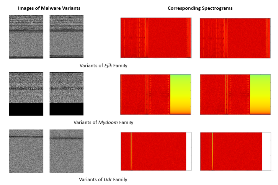
Figure 3: Visualizations of malware variants as grayscale images (left) and their corresponding audio spectrograms (right) belonging to Ejik, Mydoom and Udr malware families. We can see that the spectrograms exhibit similarity for malware variants belonging to the same family, and are different from those of other families (images and spectrograms are scaled approximately to the same size for visualization).

N-grams of Bytes: n-grams of byte codes have been effective in classifying and detecting malware [16]. As an example, for the byte stream ‘0a 1b c4 8a’, the corresponding 2-grams (bigrams) will be 0a1b, 1bc4, c48a. We use the 2-grams frequency count to obtain a $2^{16}$ (65,536-D) feature vector.

N-grams of Disassembled Instructions: Apart from n-grams of bytes, n-grams of disassembled instructions are also good features to characterize malware [17]. We use the simple objdump tool for disassembly. Figure 2 shows the disassembly for two variants of Alueron family. We see that most of the instructions are similar. We will use the instruction count of 46 most common instructions as our feature vector.

pehash: This method utilizes Portable Executable (PE) file structure characteristics and computes a hash to cluster polymorphic malware variants [18]. This is based on the assumption that polymorphic malware share the same PE file structure properties. Attributes such as image characteristics, heap commit size, stack commit size, virtual address, raw size and section characteristics are used to compute a 40-character long hash. For example, hash values of two variants from Adialer malware family will be:
Variant 1: dbf2a2ef1fed22c6e20ffa1b9a5ab69a75c365eb
Variant 2: dbf2a2ef1fed22c6e20ffa1b9a5ab69a75c365eb

Since the hash value is the same, the number of collisions between different hashes in a database is used to compute similarity. To facilitate faster processing and distance computation, we convert the characters to their ASCII value and obtain a 40-D pehash feature vector for every sample.

III Methodology and Experiments

III-A Similarity of malware when represented as audio signals

We have previously shown that malware variants exhibit visual similarity when represented as digital images [1, 19]. Here, a malware binary is read as a one dimensional signal of 8-bit unsigned integers, where every entry is a byte value of the malware. The range of this signal is $[0,255]$. In Fig 3, we notice this similarity even in the audio signals when visualized as spectrograms (time vs frequency) for malware variants belonging to Ejik, Mydoom and Udr families. These spectrograms are similar for variants within a family while different from variants of other families. For comparison, the grayscale images of these samples are also shown in Fig 3. This motivated us to explore audio similarity descriptors for malware detection. We investigated the following audio descriptors that are commonly used in audio and music analysis using the librosa package [20]:

• Chroma: This feature projects the audio spectrum into 12 bins corresponding to distinct semitones (or chroma) within the musical octave. This feature exploits the fact that humans perceive notes that are one octave apart similarly. Hence understanding the characteristic of a musical piece within an octave helps identify musical similarity. The librosa package provides 3 variations for calculating Chroma features:

  • Chroma-STFT: The first option uses short term fourier transform (STFT) to get the audio spectrum.

  • Chroma-CQT: The second option uses constant Q-transform (CQT) [21] to get the audio spectrum.

  • Chroma-CENS: The third option employs an additional step of energy normalization to get chroma energy normalized statistics (CENS) [22].

• Mel Frequency Cepstral Coefficients (MFCC): This feature captures the shape of the spectral envelope in 20 coefficients to form a 20-dimensional (20-D) feature vector. The MFCC are obtained by first calculating the power spectrum from STFT, then mapping these to mel scale using triangular windows (to mimic the human auditory system), then taking log of these mel scale power coefficients, and finally taking the discrete cosine transform of these log mel power coefficients. The MFCC are popular features for speech recognition as the spectral envelope shape can distinguish between different phenoms of speech [23].

• Melspectrogram: This feature is similar to MFCC, wherein the magnitude spectrum is first calculated using STFT and then mapped to mel scale using 128 triangular windows. These coefficients capture more detailed frequency information compared to only spectral envelope shape of MFCC.

III-A1 Preliminary experiments using MFCC features

As a preliminary experiment, we used the Malimg dataset which contains variants from 25 malware families [1]. The dataset has a mixture of both packed and unpacked malware and the number of samples per family varies from 80 to 2,949. We first convert them to audio signals and compute MFCC features. Using 10-fold cross validation, we divide the data into 10 disjoint folds and chose 9 folds for training, 1 fold for testing and then vary the folds for 10 iterations. The classification accuracy is then obtained for each iteration and then averaged over all iterations. The Nearest Neighbor classifier is used for classification. For this experiment, we obtained a high classification accuracy of 97%, thus showing that audio descriptors are able to correctly classify most families as shown in Figure 4.

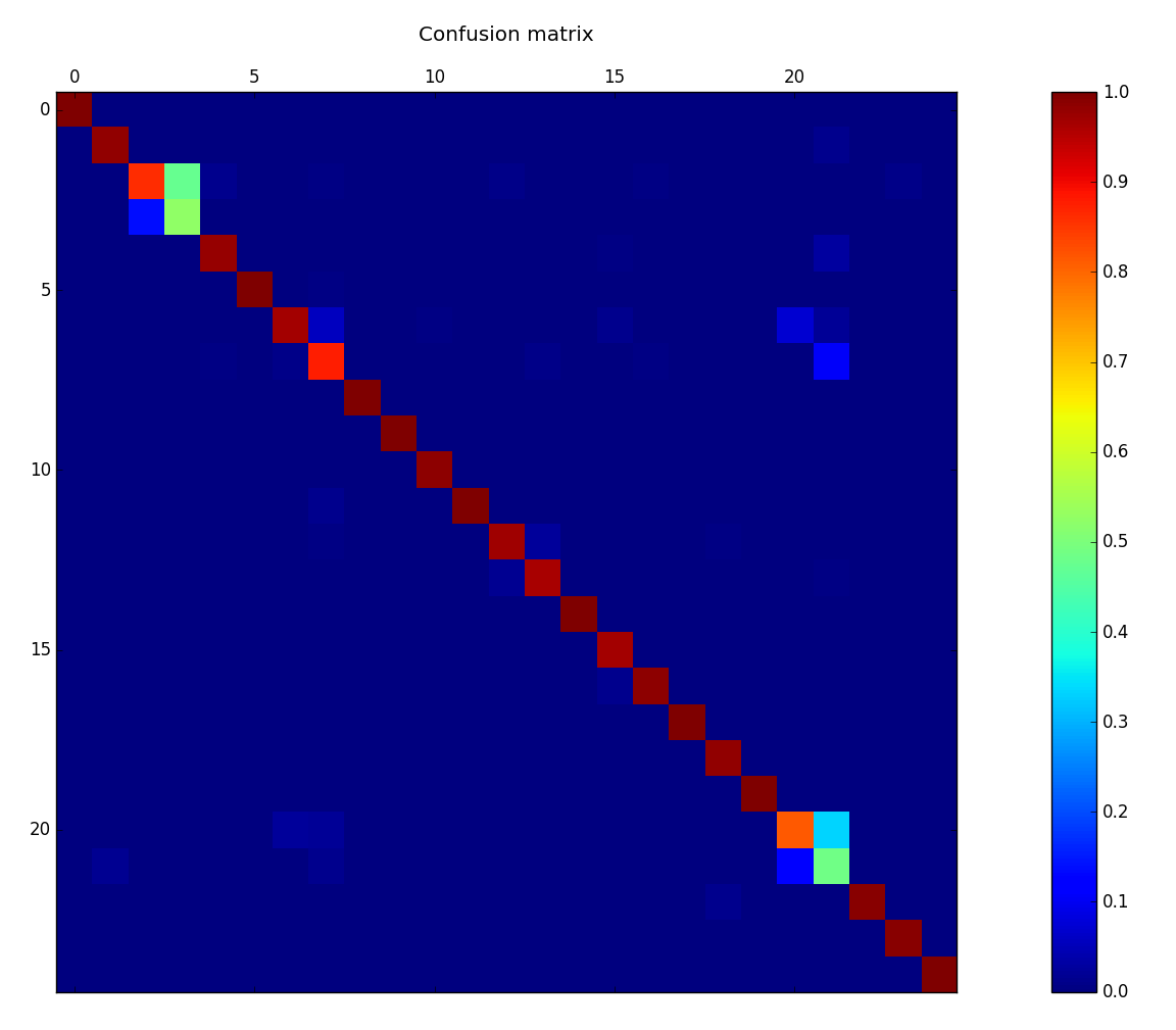
Figure 4: Confusion matrix for malware classification of different families using MFCC features.

We also setup another experiment where the objective is to verify if MFCC features (20-D) can identify malware samples from benign samples. Here, we append the Malimg dataset with benign system files from different versions of Windows Operating systems. In this way, we generated a small dataset with 9,130 samples from MalImg dataset [1] + 7,228 benign samples from Windows system files. To evaluate orthogonality, we perform a comparative assessment of MFCC features with various feature sets previously used for malware detection:

• GIST descriptors based on image similarity (320-D)

• n-grams of byte codes (65,536-D)

• Assembly Language Instruction count (46-D)

• pehash (128-D)

Using Nearest Neighbor classifier, we compare the classification accuracy of all the feature sets using 10-fold cross validation. The results are shown in Table I. We see that the accuracy of MFCC features is comparable with n-grams, instruction count and GIST but outperforms pehash. We note that the 20-D MFCC features are very compact, compared to n-grams that is 3,000 times larger at 65,536-D, or the 320-D GIST features. We do not consider the byte n-grams feature in our future experiments due to it’s large computational footprint. For 46-D instruction count feature, though the 20-D MFCC feature is comparable in size, the binary needs to be disassembled. This is challenging since malware are known to be designed with anti-disassembly mechanisms [24] to evade reverse engineering. On our dataset 209 malware could not be disassembled. But this problem will not arise for MFCC features since it directly works on the bytes. The concise representation of MFCC features, while maintaining similar/superior performance, points to a difference in underlying information used, and thus shows orthogonality.

TABLE I: Comparison of Accuracy of MFCC features.

n-grams	ins count	pehash	gist	MFCC
0.9937	0.9964	0.9461	0.9957	0.9887

III-A2 Error analysis showing signs of orthogonality

To further evaluate orthogonality, we performed an error analysis to see if MFCC features can correctly identify samples that were misclassified by other feature sets (and vice-versa). The number of incorrectly classified samples (errors) were 33 for n-grams, 23 for instruction count, 49 for GIST and 68 for MFCC features. Among these samples, MFCC features had an error overlap of 5 samples with n-grams, 4 with instruction count, 1,397 with pehash and 6 with GIST features. This shows that MFCC features correctly identified 28 samples (33-5) that were misclassified by n-grams, while n-grams correctly identified 63 samples (68-5) that were misclassified by MFCC features, thus establishing that these two feature sets can make predicitons that are orthogonal to each other. Thus, in Table II, we see that MFCC features correctly classified 28 samples against n-grams, 19 against instruction count, 43 samples against GIST and 1,374 against pehash. This strengthens the argument of the orthogonality of MFCC features.

TABLE II: Samples correctly classified by MFCC features but misclassified by other feature sets and vice versa.

	n-grams	ins count	pehash	gist
MFCC $\checkmark$, Others $\times$	28	19	1,374	43
MFCC $\times$, Others $\checkmark$	63	64	45	62

III-B Orthogonality metric

To further understand these results and to measure their orthogonality with respect to other feature sets, we use a metric called the “Joint Feature Score ($JFS$)” that we had previously used in [5]. To calculate $JFS$, we first calculate the error-analysis matrix, $E$, that compares classification errors for different feature sets. Specifically, $i$th row in this matrix corresponds to one feature set-$i$, and the $j$th column in this row corresponds to the number of samples that were misclassified by the feature set-$i$ but were correctly classified by feature set-$j$. We then normalize row $i$ by the number of samples misclassified by feature set-$i$ to generate normalized error-analysis matrix, $E_{N}$. If two feature sets $i,j$ ($i\neq j$) are orthogonal, i.e., errors using feature set-$i$ are completely different from those for feature set-$j$, then the normalized error matrix will have entries ‘1’ in for $(i,j)$ and $(j,i)$. Using this criteria we define the ($JFS$) between feature sets $i$ and $j$ as

$$JFS(i,j)=(2-\left((1-E_{N}(i,j))^{2}+(1-E_{N}(j,i))^{2}\right)^{1/2})/2$$ (1)

Clearly, if the feature sets are orthogonal, $JFS$ will be 1, and if their errors overlap completely, then it will be 0.

TABLE III: Classification accuracies when using audio descriptors on the small dataset.

	k-NN	RF	MLP	AdaBoost
MFCCe (320d)	0.9932	0.9931	0.9963	0.9873
Melspectrogram (384d)	0.9786	0.9961	0.9953	0.9929
Chroma-STFT (312d)	0.9550	0.9761	0.9663	0.9506
Chroma-CQT (312d)	0.9196	0.9370	0.9560	0.8798
Chroma-CENS (312d)	0.8852	0.9360	0.9416	0.8640

TABLE IV: Number of classification errors for different feature sets on the small dataset.

Features	Accuracy	# incorrectly classified samples
		(out of 1,636)
gist (320d)	0.9951	8
instrcount (46d)	0.9969	5
pehash (40d)	0.9113	145
MFCCe (320d)	0.9932	11

TABLE V: Error analysis for feature sets on the small dataset.

Error	gist	instrcount	pehash	MFCCe
gist	-	8	6	6
instrcount	5	-	2	5
pehash	143	142	-	144
MFCCe	9	11	10	-

TABLE VI: $JFS$ score matrix comparing orthogonality of different feature sets on the small dataset – normalization factors are derived from the last column of Table IV.

$JFS$ Score	gist	instrcount	pehash	MFCCe
gist	-	1	0.88	0.85
instrcount	1	-	0.7	1
pehash	0.88	0.7	-	0.95
MFCCe	0.85	1	0.95	-

III-C Experimental results using extended audio features

Here, we further extend the audio features by averaging the features for uniform divided parts of the binary files. This allows us to capture local variations in features across the file, which enabled better classification accuracy than the non-extended features. The expansion in features is chosen such that the number of dimensions is close to the GIST image feature of 320. Specifically, for MFCC we divide the binary file into 16 equal parts to get $16\times 20=320$ values, and refer to these extended features as MFCCe. Similarly, for Melspectrogram we divide into 3 parts to get $128\times 3=384$ values; and for chroma we divide into 26 parts to get $12\times 26=312$ values. We pass these features to 4 different ML classifiers of k-nearest neighbor (k-NN), random forest (RF), deep neural network based machine learning predictor (MLP), and AdaBoost. The experimental results (with one byte per sample) on the small dataset with 10-fold cross validation are presented in Table III. Clearly, increased feature dimensions improves classification accuracy. Particularly performance using MFCCe is now close to that obtained using image GIST feature. These are encouraging results given that we have previously observed that classification using these two feature sets are quite orthogonal to each other. The errors corresponding to different feature sets with k-NN classifier (k=1) are listed in Table IV. The error analysis matrix ($E$) for these feature sets is shown in Table V. The $JFS$ score for each pair of feature sets is shown in Table VI. Clearly, these scores indicate that audio features are orthogonal to other feature types. Next, we validate our approach on a larger dataset to see if our approach is scalable.

TABLE VII: Classification accuracies when using audio descriptors on the MaleX dataset.

	k-NN	RF	MLP	AdaBoost
MFCCe (320d)	0.9032	0.9121	0.8909	0.8477
Melspectrogram (384d)	0.9026	0.9034	0.9016	0.8407
Chroma-STFT (312d)	0.8424	0.8858	0.8561	0.8422
Chroma-CQT (312d)	0.8155	0.8786	0.8592	0.8401
Chroma-CENS (312d)	0.8423	0.8776	0.8621	0.8391

TABLE VIII: Number of classification errors for different feature sets on MaleX.

Features	Accuracy	# incorrectly classified samples
		(out of 104,440)
gist (320d)	0.8888	11,611
instrcount (46d)	0.9175	8,613
pehash (40d)	0.8867	11,835
MFCCe (320d)	0.9032	10,107

TABLE IX: Error analysis for feature sets on MaleX.

Error	gist	instrcount	pehash	MFCCe
gist	-	7,087	5,601	5,335
instrcount	4,089	-	3,804	4,227
pehash	5,825	7,026	-	6,234
MFCCe	3,831	5,721	4,506	-

TABLE X: $JFS$ score matrix comparing orthogonality of different feature sets on MaleX – normalization factors are derived from the last column of Table VIII.

$JFS$ Score	gist	instrcount	pehash	MFCCe
gist	-	0.67	0.64	0.59
instrcount	0.67	-	0.65	0.67
pehash	0.64	0.65	-	0.64
MFCCe	0.59	0.67	0.64	-

III-D Large scale analysis on MaleX dataset

We validate our approach on the bigger MaleX [5] dataset, which contains 179,725 benign samples and 864,669 malicious samples (both packed and unpacked) pertaining to Windows OS. We follow the same procedure as the previous experiment and and the results are shown in Table VII. The errors corresponding to different feature sets of the MaleX dataset (179,725 benign and 864,669 malicious samples) when using random-forest classifier is listed in Table VIII (results were similar for other classifiers too). The error analysis matrix ($E$) for these feature sets is shown in Table IX. The $JFS$ score for each pair of feature sets is shown in Table X. As we can see from these results, our approach is scalable even on a dataset that is 66 times larger (1 million samples).

IV Discussion

Observation 1 – Orthogonality test helps in better fusion of feature sets: The orthogonality test checks if new feature sets help in identifying malware samples that are not already identified by existing features; thus an analyst can decide a go/no-go on a new feature set. Now, the question could be asked if we could combine the predictions of the feature sets that passed the test and build another meta-classifier. We performed this experiment for the feature sets in Table I with the Nearest Neighbor classifier and obtained a fusion accuracy of 99.98% (0.3% improvement over the feature with highest accuracy and 5% improvement over the feature with lowest accuracy). This shows that there is scope for improvement after passing the orthogonality test and it could be left to the analyst to decide if the analyst would like to keep the individual feature predictions or the fused prediction result.

Observation 2 – The choice of machine learning (ML) classifiers has a minimal impact on performance: From our experimental results both on the small dataset and the MaleX dataset, we observe that the choice of our ML classifier has negligible impact on the accuracy of the features. Hence, this choice can be left to an analyst depending on the use case. For example, in certain defense/military applications, use of Nearest Neighbor classifier is preferable since the prediction can easily be mapped to the nearest neighbor and the distance to it, thus providing some explainability and confidence.

Observation 3 – OMD framework is generalizable to other features: We primarily focused on feature sets that are computed fast (milliseconds to seconds) such as static and signal processing (audio and image) features. We picked these features as a proof of concept for our overall framework of error analysis and orthogonality test. This does not stop an analyst from adding complex feature sets based on dynamic analysis, which could take longer time to compute (minutes to hours), but could easily be added to our framework, once the predictions from these features have been completed.

Observation 4 – $JFS$ is sensitive to class imbalance: The $JFS$ metric used to determine orthogonality between a pair of feature sets shows better resilience when the class distribution is balanced. For example, Table XI shows the results for a balanced subset of MaleX dataset that contains 179,725 benign and 179,725 randomly sampled malware samples from the full Malex dataset. These results better support the orthogonality claims made for various pairs of the feature sets similar to that of the somewhat-balanced small dataset (Table VI). However, these results are slightly different when compared to that of the entire MaleX dataset (Table X) which has more malware samples. This suggests that while using the $JFS$ metric for orthogonality measure, it is worthwhile to consider a more balanced data setup which can be obtained using any random sampling strategy that maintains the data diversity.

TABLE XI: $JFS$ score matrix comparing orthogonality of different feature sets on a balanced subset of MaleX dataset.

$JFS$ Score	gist	instrcount	pehash	MFCCe
gist	-	0.75	0.76	0.66
instrcount	0.75	-	0.78	0.75
pehash	0.76	0.78	-	0.75
MFCCe	0.66	0.75	0.75	-

V Conclusion and Future Work

In this paper, we proposed a novel framework for orthogonal malware detection (OMD) using features based on audio, image, and static analysis. We showed that audio descriptors are effective in detecting and classifying malware, and the predictions made on the audio descriptors are orthogonal to the predictions made on other feature sets. We evaluated our approach using an orthogonality metric which quantifies how orthogonal a new feature set is with respect to other feature sets. Thus our overall framework and approach can be easily extended and adapted to allow new features and detection methods to be added. In future, we will develop a malware informatics engine which integrates signal/image based malware techniques with standard security methods and provide insights both from a signal/image and security point of view.

References

- [1] L. Nataraj, S. Karthikeyan, G. Jacob, and B. Manjunath, “Malware images: visualization and automatic classification,” in Proc. International symposium on visualization for cyber security. ACM, 2011, p. 4.
- [2] L. Nataraj and B. Manjunath, “Spam: Signal processing to analyze malware [applications corner],” IEEE Signal Processing Magazine, vol. 33, no. 2, pp. 105–117, 2016.
- [3] R. Vinayakumar, M. Alazab, K. Soman, P. Poornachandran, and S. Venkatraman, “Robust intelligent malware detection using deep learning,” IEEE Access, vol. 7, pp. 46 717–46 738, 2019.
- [4] D. Gibert, C. Mateu, and J. Planes, “The rise of machine learning for detection and classification of malware: Research developments, trends and challenges,” Journal of Network and Computer Applications, 2020.
- [5] T. M. Mohammed, L. Nataraj, S. Chikkagoudar, S. Chandrasekaran, and B. Manjunath, “Malware detection using frequency domain-based image visualization and deep learning,” in Proceedings of the 54th Hawaii International Conference on System Sciences, 2021, p. 7132.
- [6] M. H. Nguyen, D. Le Nguyen, X. M. Nguyen, and T. T. Quan, “Auto-detection of sophisticated malware using lazy-binding control flow graph and deep learning,” Computers & Security, vol. 76, pp. 128–155, 2018.
- [7] Z. Ma, H. Ge, Y. Liu, M. Zhao, and J. Ma, “A combination method for android malware detection based on control flow graphs and machine learning algorithms,” IEEE access, vol. 7, pp. 21 235–21 245, 2019.
- [8] H. Zhang, X. Xiao, F. Mercaldo, S. Ni, F. Martinelli, and A. K. Sangaiah, “Classification of ransomware families with machine learning based on n-gram of opcodes,” Future Generation Computer Systems, 2019.
- [9] A. P. Namanya, I. U. Awan, J. P. Disso, and M. Younas, “Similarity hash based scoring of portable executable files for efficient malware detection in iot,” Future Generation Computer Systems, 2020.
- [10] T. Rezaei and A. Hamze, “An efficient approach for malware detection using pe header specifications,” in 2020 6th International Conference on Web Research (ICWR). IEEE, 2020, pp. 234–239.
- [11] J. Zhang, Z. Qin, H. Yin, L. Ou, S. Xiao, and Y. Hu, “Malware variant detection using opcode image recognition with small training sets,” in 2016 25th International Conference on Computer Communication and Networks (ICCCN). IEEE, 2016, pp. 1–9.
- [12] M. Farrokhmanesh and A. Hamzeh, “A novel method for malware detection using audio signal processing techniques,” in 2016 Artificial Intelligence and Robotics (IRANOPEN). IEEE, 2016, pp. 85–91.
- [13] P. Sharma and A. Raglin, “Image-audio encoding for information camouflage and improving malware pattern analysis,” in 2018 17th IEEE International Conference on Machine Learning and Applications (ICMLA). IEEE, 2018, pp. 1059–1064.
- [14] A. Azab and M. Khasawneh, “Msic: malware spectrogram image classification,” IEEE Access, vol. 8, pp. 102 007–102 021, 2020.
- [15] F. Mercaldo and A. Santone, “Audio signal processing for android malware detection and family identification,” Journal of Computer Virology and Hacking Techniques, vol. 17, no. 2, pp. 139–152, 2021.
- [16] J. Z. Kolter and M. A. Maloof, “Learning to detect and classify malicious executables in the wild,” JLMR, 2006.
- [17] A. Lakhotia, A. Walenstein, C. Miles, and A. Singh, “Vilo: a rapid learning nearest-neighbor classifier for malware triage,” Journal of Computer Virology and Hacking Techniques, vol. 9, no. 3, 2013.
- [18] G. Wicherski, “pehash: A novel approach to fast malware clustering,” in 2nd USENIX Workshop on LEET, 2009.
- [19] L. Nataraj, V. Yegneswaran, P. Porras, and J. Zhang, “A comparative assessment of malware classification using binary texture analysis and dynamic analysis,” in AISec, Oct 2011.
- [20] B. McFee, C. Raffel, D. Liang, D. P. Ellis, M. McVicar, E. Battenberg, and O. Nieto, “librosa: Audio and music signal analysis in python,” in Proceedings of the 14th Python in Science Conference, 2015.
- [21] C. Schörkhuber and A. Klapuri, “Constant-q transform toolbox for music processing,” in Proceedings of the International Conference on Music Information Retrieval (ISMIR), 2010.
- [22] M. Müller, F. Kurth, and M. Clausen, “Audio matching via chroma-based statistical features.” in Proceedings of the International Conference on Music Information Retrieval (ISMIR), 2005, pp. 288–295.
- [23] L. R. Rabiner and B. H. Juang, Fundamentals of Speech Recognition. Prentice Hall, 1993.
- [24] R. R. Branco, G. N. Barbosa, and P. D. Neto, “Scientific but not academical overview of malware anti-debugging, anti-disassembly and anti-vm technologies,” Blackhat USA, vol. 12, 2012.