SMU: smooth activation function for deep networks using smoothing maximum technique

Abstract

Deep learning researchers have a keen interest in proposing two new novel activation functions which can boost network performance. A good choice of activation function can have significant consequences in improving network performance. A handcrafted activation is the most common choice in neural network models. ReLU is the most common choice in the deep learning community due to its simplicity though ReLU has some serious drawbacks. In this paper, we have proposed a new novel activation function based on approximation of known activation functions like Leaky ReLU, and we call this function Smooth Maximum Unit (SMU). Replacing ReLU by SMU, we have got 6.22% improvement in the CIFAR100 dataset with the ShuffleNet V2 model.

Keywords Smooth Activation Function  $\cdot$ Deep Learning  $\cdot$ Neural Network

1 Introduction

Deep Neural network has emerged a lot in recent years and has significantly impacted our real-life applications. Neural networks are the backbone of deep learning. An activation function is the brain of the neural network, which plays a central role in the effectiveness & training dynamics of deep neural networks. Hand-designed activation functions are quite a common choice in neural network models. ReLU [1] is a widely used hand-designed activation function. Despite its simplicity, ReLU has a major drawback, known as the dying ReLU problem in which up to 50% neurons can be dead during network training. To overcome the shortcomings of ReLU, a significant number of activations have been proposed in recent years, and Leaky ReLU [2], Parametric ReLU [3], ELU [4], Softplus [5], Randomized Leaky ReLU [6] are a few of them though they marginally improve performance of ReLU. Swish [7] is a non-linear activation function proposed by the Google brain team, and it shows some good improvement of ReLU. GELU [8] is an another popular smooth activation function. It can be shown that Swish and GELU both are a smooth approximation of ReLU. Recently, a few non-linear activations have been proposed which improves the performance of ReLU, Swish or GELU. Some of them are either hand-designed or smooth approximation of Leaky ReLU function, and Mish [9], ErfAct [10], Padé activation unit [11], Orthogonal Padé activation unit [12] are a few of them.

2 Related Work and Motivation

In a deep neural network, activations are either fixed before training or trainable. Researchers have proposed several activations in recent years by combining known functions. Some of these functions have hyperparameters or trainable parameters. In the case of trainable activation functions, parameters are optimized during training. Swish is a popular activation function that can be used as either a constant or trainable activation function, and it shows some good performance in a variety of deep learning tasks like image classification, object detection, machine translation etc. GELU shares similar properties like the Swish activation function, and it gains popularity in the deep learning community due to its efficacy in natural language processing tasks. GELU has been used in BERT [13], GPT-2 [14], and GPT-3 [15] architectures. Padé activation unit (PAU) has been proposed recently, and it is constructed from the approximation of the Leaky ReLU function by rational polynomials of a given order. Though PAU improves network performance in the image classification problem over ReLU, its variants, and Swish, it has a major drawback. PAU contains many trainable parameters, which significantly increases the network complexity and computational cost.

Motivated from these works, we propose activation functions using the smoothing maximum technique. The maximum function is non-smooth at the origin. We want to explore how the smooth approximation of the maximum function (which can be used as an activation function) affects a network’s training dynamics and performance. Our experimental evaluation shows that our proposed activation functions are comparatively more effective than ReLU, Mish, Swish, GELU, PAU etc., across different deep learning tasks. We summarise the paper as follows:

1. We have proposed activation functions by smoothing the maximum function. We show that it can approximate GELU, ReLU, Leaky ReLU or the general Maxout family.

2. We show that the proposed functions outperform widely used activation functions in a variety of deep learning tasks.

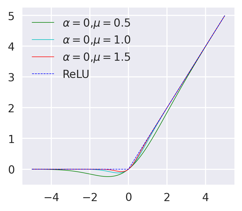
Figure 1: Approximation of ReLU using SMU ($\alpha=0$) for different values of $\mu$. As $\mu\rightarrow\infty$, SMU smoothly approximate ReLU

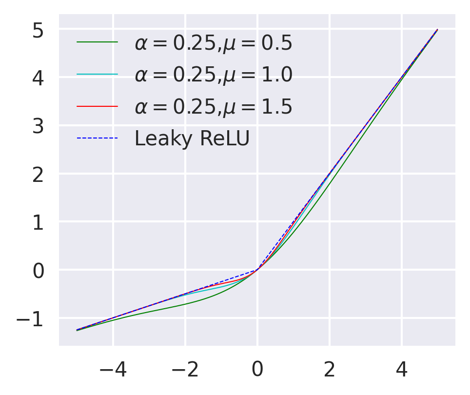
Figure 2: Approximation of Leaky ReLU ($\alpha=0.25$) using SMU for different values of $\mu$. As $\mu\rightarrow\infty$, SMU smoothly approximate Leaky ReLU

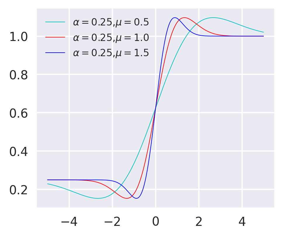
Figure 3: First order derivatives of SMU for $\alpha=0.25$ and different values of $\mu$.

3 Smooth Maximum Unit

We present Smooth Maximum Unit (SMU), smooth activation functions from the smooth approximation of the maximum function. Using the smooth approximation of the $|x|$ function, one can find a general approximating formula for the maximum function, which can smoothly approximate the general Maxout[16] family, ReLU, Leaky ReLU or its variants, Swish etc. We also show that the well established GELU [8] function can be obtained as a special case of SMU.

3.1 Smooth approximation of the maximum function

Note that the maximum function can be expressed as following two different ways:

$$max(x_{1},x_{2}) =\begin{cases}x_{1}&\text{ if }x_{1}\geq x_{2}\\ x_{2}&\text{otherwise}\end{cases}$$

$$=\frac{(x_{1}+x_{2})+|x_{1}-x_{2}|}{2}$$ (1)

Note that the max function is not differentiable at the origin. Using approximations of the $|x|$ function by a smooth function, we can create approximations to the maximum functions. There are many known approximations to $|x|$, but for the rest of this article, we will focus on two specific approximations of $|x|$, namely $x\text{erf}(\mu x)$ and $\sqrt{x^{2}+{\mu}^{2}}$. We noticed that the activations constructed using these two functions provide good performance on standard datasets on different deep learning problems (for more details, see the supplementary section). Note that $\sqrt{x^{2}+{\mu}^{2}}$ as $\mu\rightarrow 0$ approximate $|x|$ from above while $x\text{erf}(\mu x)$. as $\mu\rightarrow\infty$ gives an approximation of $|x|$ from below. The approximation is uniform on compact subsets of the real line. Here $\operatorname{erf}$ is the Gaussian error function defined as follows:

$$\operatorname{erf}(x)=\dfrac{2}{\sqrt{\pi}}\int_{0}^{x}e^{-t^{2}}\,dt.$$

Now, replacing the $|x|$ function by $x\text{erf}(\mu x)$ in equation (3.1), we have the smooth approximation formula for maximum function as follows:

$$f_{1}(x_{1},x_{2};\mu)=\frac{(x_{1}+x_{2})+(x_{1}-x_{2})\ \text{erf}(\mu(x_{1}-x_{2}))}{2}.$$ (2)

Similarly, we can derive the the smooth approximation formula for the maximum function from equation (3.1) by replacing the $|x|$ function by $\sqrt{x^{2}+{\mu}^{2}}$ as follows:

$$f_{2}(x_{1},x_{2};\mu)=\frac{(x_{1}+x_{2})+\sqrt{(x_{1}-x_{2})^{2}+\mu^{2}}}{2}$$ (3)

Note that as $\mu\rightarrow\infty$, $f_{1}(x_{1},x_{2};\mu)\rightarrow$ max$(x_{1},x_{2})$ and as $\mu\rightarrow 0$, $f_{2}(x_{1},x_{2};\mu)\rightarrow$ max$(x_{1},x_{2})$. For particular values of $x_{1}$ and $x_{2}$, we can approximate known activation functions. For example, consider $x_{1}=ax$, $x_{2}=bx$, with $a\neq b$ in (2), we get:

$$f_{1}(ax,bx;\mu)=\frac{(a+b)x+(a-b)x\ \text{erf}(\mu(a-b)x)}{2}.$$ (4)

This is a simple case from the Maxout family [16] while more complicated cases can be found by considering nonlinear choices of $x_{1}$ and $x_{2}$. We can similarly get smooth approximations to ReLU and Leaky ReLU. For example, consider $x_{1}=x$ and $x_{2}=0$, we have smooth approximation of ReLU as follows:

$$f_{1}(x,0;\mu)=\frac{x+x\ \text{erf}(\mu x)}{2}.$$ (5)

We know that GELU [8] is a smooth approximation of ReLU. Notice that, if we choose $\mu=\frac{1}{\sqrt{2}}$ in equation (5), we can recover GELU activation function which also show that GELU is smooth approximation of ReLU. Also, considering $x_{1}=x$ and $x_{2}=\alpha x$, we have a smooth approximation of Leaky ReLU or Parametric ReLU depending on whether $\alpha$ is a hyperparameter or a learnable parameter.

$$f_{1}(x,\alpha x;\mu)=\frac{(1+\alpha)x+(1-\alpha)x\ \text{erf}(\mu(1-\alpha)x)}{2}.$$ (6)

Note that, equation (5) and equation (6) approximate ReLU or Leaky ReLU from below. Similarly, we can derive approximating function from equation (3) which will approximate ReLU or Leaky ReLU from above.

The corresponding derivatives of equation (6) for input variable $x$ is

$$\frac{d}{dx}f_{1}(x,\alpha x;\mu)=\frac{1}{2}[(1+\alpha)+(1-\alpha)\ \text{erf}(\mu(1-\alpha)x)$$

$$+\frac{2}{\sqrt{\pi}}\mu(1-\alpha)^{2}xe^{-(\mu(1-\alpha)x)^{2}}]$$ (7)

$$\text{where}\ \ \frac{d}{dx}\text{erf}(x)=\frac{2}{\sqrt{\pi}}e^{-x^{2}}.\quad\quad\quad\quad\quad\quad\quad\quad\quad\quad\quad$$

Figures 3,  3, and  3 show the plots for $f_{1}(x,0;\mu)$, $f_{1}(x,0.25x;\mu)$, and derivative of $f_{1}(x,0.25x;\mu)$ for different values of $\mu$. From the figures it is clear that as $\mu\rightarrow\infty$, $f_{1}(x,\alpha x;\mu)$ smoothly approximate ReLU or Leaky ReLU depending on value of $\alpha$. We call the function in equation (6) as Smooth Maximum Unit (SMU). Similarly, We can derive a function by replacing $x_{1}=x$ and $x_{2}=\alpha x$ in equation (3) and we call this function SMU-1. For all of our experiments, we will use SMU and SMU-1 as our proposed activation functions.

3.2 Learning activation parameters via back-propagation

Trainable activation function parameters are updated using backpropagation [17] technique. We implemented forward pass in both Pytorch [18] & Tensorflow-Keras [19] API, and automatic differentiation will update the parameters. Alternatively, CUDA [20] based implementation (see [2]) can be used and the gradients of equations 8 and 9) for the parameters $\alpha$ and $\mu$ can be computed as follows:

$$\frac{\partial f_{1}}{\partial\alpha}=\frac{1}{2}[x-x\ \text{erf}(\mu(1-\alpha)x)-(1-\alpha)\mu x^{2}e^{-(\mu(1-\alpha)x)^{2}}]$$ (8)

$$\frac{\partial f_{1}}{\partial\mu}=\frac{1}{2}(1-\alpha)^{2}x^{2}e^{-(\mu(1-\alpha)x)^{2}}$$ (9)

$\alpha$ and $\mu$ can be either hyperparameters or trainable parameters. For classification problem, we consider $\alpha=0.25$, a hyperparameter. We consider $\mu$ as trainable parameter and initialise at $1.0$ and $4.352665993287951e^{-09}$ for SMU and SMU-1 respectively. For object detection and semantic segmentation problem, we consider $\alpha=0.01$, a hyperparameter. We consider $\mu$ as trainable parameter and initialise at $2.5$ and $4.332461424154261e-09$ for SMU and SMU-1 respectively.
Now, note that the class of neural networks with SMU and SMU-1 activation function is dense in $C(K)$, where $K$ is a compact subset of $\mathbb{R}^{n}$ and $C(K)$ is the space of all continuous functions over $K$.
The proof follows from the following proposition (see [11]).

Proposition 1. (Theorem 1.1 in Kidger and Lyons, 2020 [21]) :- Let $\rho:\mathbb{R}\rightarrow\mathbb{R}$ be any continuous function. Let $N_{n}^{\rho}$ represent the class of neural networks with activation function $\rho$, with $n$ neurons in the input layer, one neuron in the output layer, and one hidden layer with an arbitrary number of neurons. Let $K\subseteq\mathbb{R}^{n}$ be compact. Then $N_{n}^{\rho}$ is dense in $C(K)$ if and only if $\rho$ is non-polynomial.

4 Experiments

In the next subsections, we will provide a detailed experimental evaluation to compare performance for our proposed activation function and some widely used activation functions on 3 different deep learning problems like image classification, object detection, and semantic segmentation.

4.1 CIFAR

We report the top-1 accuracy on Table 1 and Table 2 on CIFAR10 [22] and CIFAR100 [22] datasets respectively. We consider MobileNet V2 [23], Shufflenet V2 [24], PreActResNet [25], ResNet [26], VGG [27] (with batch-normalization [28]), and EfficientNet B0 [29].

Model ReLU SMU SMU-1 Top-1 accuracy Top-1 accuracy Top-1 accuracy ShuffleNet V2 1.0x 90.81 $\pm$ 0.24 92.72 $\pm$ 0.18 92.42 $\pm$ 0.20 ShuffleNet V2 2.0x 91.70 $\pm$ 0.20 93.61 $\pm$ 0.14 93.40 $\pm$ 0.16 PreActResNet 34 94.21 $\pm$ 0.17 95.12 $\pm$ 0.13 94.93 $\pm$ 0.14 ResNet 34 94.22 $\pm$ 0.18 94.91 $\pm$ 0.16 94.77 $\pm$ 0.17 SeNet 34 94.42 $\pm$ 0.20 95.27 $\pm$ 0.15 94.89 $\pm$ 0.17 MobileNet V2 94.22 $\pm$ 0.15 95.50 $\pm$ 0.09 95.27 $\pm$ 0.10 EffitientNet B0 95.10 $\pm$ 0.15 96.23 $\pm$ 0.10 96.11 $\pm$ 0.12 Xception 90.51 $\pm$ 0.22 93.25 $\pm$ 0.17 92.59 $\pm$ 0.20 VGG16 93.59 $\pm$ 0.18 94.54 $\pm$ 0.14 93.32 $\pm$ 0.15

Table 1: Comparison between our proposed activations and other baseline activations in the CIFAR10 dataset. We report the results for the mean of 15 different runs. mean$\pm$std is reported in the table.

Model ReLU SMU SMU-1 Top-1 accuracy Top-1 accuracy Top-1 accuracy Shufflenet V2 1.0x 64.41 $\pm$ 0.25 70.60 $\pm$ 0.21 69.96 $\pm$ 0.22 Shufflenet V2 2.0x 67.52 $\pm$ 0.25 73.74 $\pm$ 0.20 73.45 $\pm$ 0.23 PreActResNet 34 73.41 $\pm$ 0.24 76.21 $\pm$ 0.20 75.87 $\pm$ 0.21 ResNet 34 73.33 $\pm$ 0.27 75.77 $\pm$ 0.20 75.59 $\pm$ 0.21 SeNet 34 75.12 $\pm$ 0.22 76.79 $\pm$ 0.18 75.79 $\pm$ 0.21 MobileNet V2 74.17 $\pm$ 0.24 76.31 $\pm$ 0.19 76.03 $\pm$ 0.19 Xception 71.22 $\pm$ 0.26 74.62 $\pm$ 0.23 74.11 $\pm$ 0.23 EffitientNet B0 76.60 $\pm$ 0.27 79.10 $\pm$ 0.22 78.77 $\pm$ 0.23 VGG16 71.87 $\pm$ 0.30 73.26 $\pm$ 0.22 72.79 $\pm$ 0.23

Table 2: Comparison between our proposed activations and other baseline activations in the CIFAR100 dataset. We report the results for the mean of 15 different runs. mean$\pm$std is reported in the table.

4.2 Object Detection

In this section, we report results on Pascal VOC dataset [30] on Single Shot MultiBox Detector(SSD) 300 [31] with VGG-16(with batch-normalization) [27] as the backbone network. We report the mean average precision (mAP) in Table 3 for the mean of 6 different runs.

Activation Function	mAP
SMU	78.1$\pm$0.09
SMU-1	77.9$\pm$0.10
ReLU	77.2$\pm$0.14
Leaky ReLU	77.2$\pm$0.18
PReLU	77.2$\pm$0.17
ReLU6	77.1$\pm$0.15
ELU	75.1$\pm$0.22
Softplus	74.2$\pm$0.25
Swish	77.3$\pm$0.11
GELU	77.3$\pm$0.12

Table 3: A detailed comparison between SMU activation and other baseline activations in Pascal VOC dataset. mean$\pm$std is reported in the table

4.3 Semantic Segmentation

We report our experimental results in this section on the popular CityScapes dataset [32]. The U-net model [33] is considered as the segmentation framework, and we report the mean of 6 different runs for Pixel Accuracy and the mean Intersection-Over-Union (mIOU) on test data on table 4.

Activation Function	Pixel Accuracy	mIOU
SMU	81.71$\pm$0.38	71.45$\pm$0.30
SMU-1	81.17$\pm$0.41	71.10$\pm$0.30
ReLU	79.49$\pm$0.46	69.31$\pm$0.28
PReLU	78.95$\pm$0.42	68.88$\pm$0.41
ReLU6	79.58$\pm$0.41	69.70$\pm$0.42
Leaky ReLU	79.41$\pm$0.41	69.64$\pm$0.42
ELU	79.48$\pm$0.50	68.19$\pm$0.40
Softplus	78.45$\pm$0.52	68.08$\pm$0.49
Swish	80.22$\pm$0.46	69.81$\pm$0.30
GELU	80.14$\pm$0.37	69.59$\pm$0.40

Table 4: A detailed comparison between SMU activation and other baseline activations in CityScapes dataset. mean$\pm$std is reported in the table.

5 Conclusion

This work uses the maximum smoothing technique to approximate Leaky ReLU, a well-established non-smooth (not differentiable at 0) function by two smooth functions. We call these two functions SMU and SMU-1, and we use them as a potential candidate for activation functions. Our experimental evaluation shows that the proposed functions beat the traditional activation functions in well-known deep learning problems and have the potential to replace them.

References

- [1] Vinod Nair and Geoffrey E. Hinton. Rectified linear units improve restricted boltzmann machines. In Johannes Fürnkranz and Thorsten Joachims, editors, Proceedings of the 27th International Conference on Machine Learning (ICML-10), June 21-24, 2010, Haifa, Israel, pages 807–814. Omnipress, 2010.
- [2] Andrew L. Maas, Awni Y. Hannun, and Andrew Y. Ng. Rectifier nonlinearities improve neural network acoustic models. In in ICML Workshop on Deep Learning for Audio, Speech and Language Processing, 2013.
- [3] Kaiming He, Xiangyu Zhang, Shaoqing Ren, and Jian Sun. Delving deep into rectifiers: Surpassing human-level performance on imagenet classification, 2015.
- [4] Djork-Arné Clevert, Thomas Unterthiner, and Sepp Hochreiter. Fast and accurate deep network learning by exponential linear units (elus), 2016.
- [5] Hao Zheng, Zhanlei Yang, Wenju Liu, Jizhong Liang, and Yanpeng Li. Improving deep neural networks using softplus units. In 2015 International Joint Conference on Neural Networks (IJCNN), pages 1–4, 2015.
- [6] Bing Xu, Naiyan Wang, Tianqi Chen, and Mu Li. Empirical evaluation of rectified activations in convolutional network, 2015.
- [7] Prajit Ramachandran, Barret Zoph, and Quoc V. Le. Searching for activation functions, 2017.
- [8] Dan Hendrycks and Kevin Gimpel. Gaussian error linear units (gelus), 2020.
- [9] Diganta Misra. Mish: A self regularized non-monotonic activation function, 2020.
- [10] Koushik Biswas, Sandeep Kumar, Shilpak Banerjee, and Ashish Kumar Pandey. Erfact and pserf: Non-monotonic smooth trainable activation functions, 2021.
- [11] Alejandro Molina, Patrick Schramowski, and Kristian Kersting. Padé activation units: End-to-end learning of flexible activation functions in deep networks, 2020.
- [12] Koushik Biswas, Shilpak Banerjee, and Ashish Kumar Pandey. Orthogonal-padé activation functions: Trainable activation functions for smooth and faster convergence in deep networks, 2021.
- [13] Jacob Devlin, Ming-Wei Chang, Kenton Lee, and Kristina Toutanova. Bert: Pre-training of deep bidirectional transformers for language understanding, 2019.
- [14] Alec Radford, Jeff Wu, Rewon Child, David Luan, Dario Amodei, and Ilya Sutskever. Language models are unsupervised multitask learners. 2019.
- [15] Tom B. Brown, Benjamin Mann, Nick Ryder, Melanie Subbiah, Jared Kaplan, Prafulla Dhariwal, Arvind Neelakantan, Pranav Shyam, Girish Sastry, Amanda Askell, Sandhini Agarwal, Ariel Herbert-Voss, Gretchen Krueger, Tom Henighan, Rewon Child, Aditya Ramesh, Daniel M. Ziegler, Jeffrey Wu, Clemens Winter, Christopher Hesse, Mark Chen, Eric Sigler, Mateusz Litwin, Scott Gray, Benjamin Chess, Jack Clark, Christopher Berner, Sam McCandlish, Alec Radford, Ilya Sutskever, and Dario Amodei. Language models are few-shot learners, 2020.
- [16] Ian J. Goodfellow, David Warde-Farley, Mehdi Mirza, Aaron Courville, and Yoshua Bengio. Maxout networks, 2013.
- [17] Y. LeCun, B. Boser, J. S. Denker, D. Henderson, R. E. Howard, W. Hubbard, and L. D. Jackel. Backpropagation applied to handwritten zip code recognition. Neural Computation, 1(4):541–551, 1989.
- [18] Adam Paszke, Sam Gross, Francisco Massa, Adam Lerer, James Bradbury, Gregory Chanan, Trevor Killeen, Zeming Lin, Natalia Gimelshein, Luca Antiga, Alban Desmaison, Andreas Köpf, Edward Yang, Zach DeVito, Martin Raison, Alykhan Tejani, Sasank Chilamkurthy, Benoit Steiner, Lu Fang, Junjie Bai, and Soumith Chintala. Pytorch: An imperative style, high-performance deep learning library, 2019.
- [19] François Chollet et al. Keras. https://keras.io, 2015.
- [20] J. Nickolls, I. Buck, M. Garland, and K. Skadron. Scalable parallel programming. In 2008 IEEE Hot Chips 20 Symposium (HCS), pages 40–53, 2008.
- [21] Patrick Kidger and Terry Lyons. Universal approximation with deep narrow networks, 2020.
- [22] Alex Krizhevsky. Learning multiple layers of features from tiny images. Technical report, University of Toronto, 2009.
- [23] Mark Sandler, Andrew Howard, Menglong Zhu, Andrey Zhmoginov, and Liang-Chieh Chen. Mobilenetv2: Inverted residuals and linear bottlenecks, 2019.
- [24] Ningning Ma, Xiangyu Zhang, Hai-Tao Zheng, and Jian Sun. Shufflenet v2: Practical guidelines for efficient cnn architecture design, 2018.
- [25] Kaiming He, Xiangyu Zhang, Shaoqing Ren, and Jian Sun. Identity mappings in deep residual networks, 2016.
- [26] Kaiming He, Xiangyu Zhang, Shaoqing Ren, and Jian Sun. Deep residual learning for image recognition, 2015.
- [27] Karen Simonyan and Andrew Zisserman. Very deep convolutional networks for large-scale image recognition, 2015.
- [28] Sergey Ioffe and Christian Szegedy. Batch normalization: Accelerating deep network training by reducing internal covariate shift, 2015.
- [29] Mingxing Tan and Quoc V. Le. Efficientnet: Rethinking model scaling for convolutional neural networks, 2020.
- [30] Mark Everingham, Luc Gool, Christopher K. Williams, John Winn, and Andrew Zisserman. The pascal visual object classes (voc) challenge. Int. J. Comput. Vision, 88(2):303–338, June 2010.
- [31] Wei Liu, Dragomir Anguelov, Dumitru Erhan, Christian Szegedy, Scott Reed, Cheng-Yang Fu, and Alexander C. Berg. Ssd: Single shot multibox detector. Lecture Notes in Computer Science, page 21–37, 2016.
- [32] Marius Cordts, Mohamed Omran, Sebastian Ramos, Timo Rehfeld, Markus Enzweiler, Rodrigo Benenson, Uwe Franke, Stefan Roth, and Bernt Schiele. The cityscapes dataset for semantic urban scene understanding, 2016.
- [33] Olaf Ronneberger, Philipp Fischer, and Thomas Brox. U-net: Convolutional networks for biomedical image segmentation, 2015.