Logarithmic corrections to $a^{2}$ scaling in lattice QCD with Wilson and Ginsparg-Wilson quarks

Abstract

We analyse the leading logarithmic corrections to the $a^{2}$ scaling of lattice artefacts in QCD, following the seminal work of Balog, Niedermayer and Weisz in the O(n) non-linear sigma model. Limiting the discussion to contributions from the action, the leading logarithmic corrections can be determined by the anomalous dimensions of mass-dimension 6 operators. These operators form a minimal on-shell basis of the Symanzik Effective Theory. We present results for non-perturbatively O($a$) improved Wilson and Ginsparg-Wilson quarks.

DESY 21-178

1 Introduction

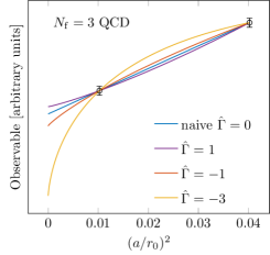
Figure 1: Sketch of the asymptotic lattice spacing dependence $a^{2}[\bar{g}^{2}(1/a)]^{\hat{\Gamma}}$ for various values of $\hat{\Gamma}$ compared to the plain $a^{2}$. We used here the 5-loop perturbative running of the QCD coupling in $\overline{\text{MS}}$ [1].

Symanzik Effective Field Theory (SymEFT) [2, 3, 4, 5] can be used to describe the lattice artifacts of lattice QCD for asymptotically small lattice spacings $a$. In contrast to the (classical) $a^{2}$ ansatz commonly used in continuum extrapolations $a\searrow 0$, the leading asymptotic lattice spacing dependence is actually of the form $a^{2}[\bar{g}^{2}(1/a)]^{\hat{\Gamma}}$ due to quantum corrections, where $\hat{\Gamma}$ is a real constant and $\bar{g}$ is the running coupling. We assume here the use of fully $\mathrm{O}(a)$ improved lattice actions throughout. Knowing $\hat{\Gamma}$ is required to put continuum extrapolations on more solid grounds and to rule out any trouble arising from distinctly negative values for $\hat{\Gamma}$ as there is no theoretical lower bound on this value. A particularly problematic example was found for the O(3) non-linear sigma model, where such an analysis [6, 7] was performed for the first time yielding $\hat{\Gamma}=-3$. To highlight the impact a non-zero $\hat{\Gamma}$ can have, we added the oversimplified sketch in fig. 1 for the case of three-flavour QCD.

2 Symanzik Effective Theory

For a more complete picture of SymEFT see [8] as we give here only a short summary of the main concepts. To describe the lattice artifacts we start from the effective Lagrangian

$$\mathscr{L}_{\mathrm{Sym}}=-\frac{1}{2g_{0}^{2}}\mathop{\mathrm{tr}}(F_{\mu\nu}F_{\mu\nu})+\bar{\Psi}\left\{\gamma_{\mu}D_{\mu}+m\right\}\Psi+a^{2}\sum_{j}c_{j}\mathcal{O}_{j}+\mathrm{O}(a^{3}),$$ (1)

which is just the (Euclidean) continuum QCD Lagrangian for $N_{\mathrm{f}}$ quark flavours $\Psi$ with additional $\mathrm{O}(a^{2})$ corrections. The matching coefficients $c_{j}$ depend on the choice for the lattice discretisation. (Only) For tree-level matching it suffices to naively expand the lattice action in the lattice spacing. The basis of operators $\mathcal{O}_{j}$ must be chosen such that it parametrises all lattice artifacts originating from the lattice action up to higher order corrections in the lattice spacing.

Being interested in either Ginsparg-Wilson (GW) or Wilson [9, 10] quarks for the lattice discretisation yields the following symmetry constraints on our minimal operator basis

• SU($N$) gauge symmetry,

• invariance under Euclidean reflections,

• invariance under charge conjugation,

• H(4) lattice symmetry, i.e. continuum O(4) symmetry is broken due to reduced rotational symmetry,

• flavour symmetries, $\mathrm{SU}(N_{\mathrm{f}})_{\mathrm{L}}\times\mathrm{SU}(N_{\mathrm{f}})_{\mathrm{R}}\times\mathrm{U}(1)$ for massless GW quarks and $\mathrm{U}(N_{\mathrm{f}})_{\mathrm{V}}$ for massless Wilson quarks.

Notice that $\mathrm{SU}(N_{\mathrm{f}})_{\mathrm{L}}\times\mathrm{SU}(N_{\mathrm{f}})_{\mathrm{R}}\times\mathrm{U}(1)\subset\mathrm{U}(N_{\mathrm{f}})_{\mathrm{V}}$ such that the minimal basis of GW quarks is a subset of the full minimal basis needed for Wilson quarks. Due to being only interested in on-shell physics we can make use of the continuum equations of motion to reduce the operator basis further [11].

The minimal on-shell operator basis for the massless case (or sufficiently small quark masses) then is the following [12, 13, 14]

$$\mathcal{O}_{1} =\frac{1}{g_{0}^{2}}\mathop{\mathrm{tr}}(D_{\mu}F_{\nu\rho}D_{\mu}F_{\nu\rho}), \mathcal{O}_{2} =\frac{1}{g_{0}^{2}}\sum_{\mu}\mathop{\mathrm{tr}}(D_{\mu}F_{\mu\nu}D_{\mu}F_{\mu\nu}),$$

$$\mathcal{O}_{3} =\sum_{\mu}\bar{\Psi}\gamma_{\mu}D_{\mu}^{3}\Psi, \mathcal{O}_{k\geq 4} =g_{0}^{2}(\bar{\Psi}\Gamma_{k}\Psi)^{2},$$ (2)

where $\Gamma_{4-7}\in\{\gamma_{\mu},\gamma_{5}\gamma_{\mu}\}\otimes\{\mathbb{1},T^{a}\}$ and $\Gamma_{8-13}\in\{\mathbb{1},\gamma_{5},\sigma_{\mu\nu}\}\otimes\{\mathbb{1},T^{a}\}$ with $\sigma_{\mu\nu}=\frac{i}{2}[\gamma_{\mu},\gamma_{\nu}]$. The operators $\mathcal{O}_{2}$ and $\mathcal{O}_{3}$ both break O(4) symmetry. For massless GW quarks we only need $\mathcal{O}_{k\leq 7}$, while massless Wilson quarks require the entire set of operators listed here. For the general massive case we get additional massive operators, that are listed and discussed in [15, 16].

3 Leading powers in the coupling

For an arbitrary Renormalisation Group invariant (RGI) spectral quantity $\mathcal{P}$ we may use the operator basis to write the leading lattice artifacts as

$$\mathcal{P}(a)=\mathcal{P}(0)-a^{2}\sum_{j}\bar{c}_{j}^{\mathcal{O}}\delta\mathcal{P}_{j}^{\mathcal{O}}(1/a)\times\left\{1+\mathrm{O}(\bar{g}^{2}(1/a))\right\}+\mathrm{O}(a^{3}),$$ (3)

where $\bar{c}_{j}^{\mathcal{O}}$ is the tree-level matching coefficient and $\delta\mathcal{P}_{j}^{\mathcal{O}}$ contains the matrix elements of interest with an additional insertion of $\int\mathrm{d}^{4}x\,\mathcal{O}_{j}(x)$. The remaining scale dependence of $\delta\mathcal{P}_{j}^{\mathcal{O}}(1/a)$, where $1/a$ is the relevant renormalisation scale for lattice artifacts, is governed by the renormalisation group equation

$$\mu\frac{\delta\mathcal{P}_{i}^{\mathcal{O}}(\mu)}{\mathrm{d}\mu}=-\left\{\gamma_{0}^{\mathcal{O}}\bar{g}^{2}(\mu)+\mathrm{O}(\bar{g}^{4})\right\}_{ij}\delta\mathcal{P}_{j}^{\mathcal{O}}(\mu),$$ (4)

where $\gamma_{0}^{\mathcal{O}}$ is the 1-loop coefficient of the anomalous dimension matrix. In general $\gamma_{0}^{\mathcal{O}}$ is not diagonal, but in our case we can make a change of basis $\mathcal{O}\rightarrow\mathcal{B}$ such that $\gamma_{0}^{\mathcal{B}}=\mathop{\mathrm{diag}}\big{(}(\gamma_{0})_{1},\ldots,(\gamma_{0})_{n}\big{)}$ becomes diagonal. In turn this allows to introduce the RGI, where all scale dependence is absorbed into some perturbatively known prefactor

$$\delta\mathcal{P}_{j}^{\mathcal{B}}(1/a)=[2b_{0}\bar{g}^{2}(1/a)]^{\hat{\gamma}_{j}}\delta\mathcal{P}_{j;\mathrm{RGI}}^{\mathcal{B}}\times\left\{1+\mathrm{O}(\bar{g}^{2}(1/a))\right\},\quad\hat{\gamma}_{j}=\frac{(\gamma_{0}^{\mathcal{B}})_{j}}{2b_{0}},$$ (5)

where $b_{0}$ is the 1-loop coefficient of the $\beta$-function and the factor $2b_{0}$ in front of $\bar{g}^{2}(1/a)$ is the common choice for the normalisation. Taking the leading order matching $c_{j}^{\mathcal{B}}(\bar{g}^{2})=\hat{c}_{j}^{\mathcal{B}}[2b_{0}\bar{g}^{2}(1/a)]^{n_{j}^{\mathrm{I}}}\times\left\{1+\mathrm{O}(\bar{g}^{2}(1/a))\right\}$ into account, we eventually arrive at the central formula for the leading asymptotic lattice spacing dependence

$$\mathcal{P}(a) =\mathcal{P}(0)-a^{2}\sum_{j}[2b_{0}\bar{g}^{2}(1/a)]^{\hat{\Gamma}_{j}}\hat{c}_{j}^{\mathcal{B}}\delta\mathcal{P}_{j;\mathrm{RGI}}^{\mathcal{B}}\times\left\{1+\mathrm{O}(\bar{g}^{2}(1/a))\right\}+\mathrm{O}(a^{3}),\quad\hat{\Gamma}_{j}=\hat{\gamma}_{j}+n_{j}^{\mathrm{I}}\,,$$ (6)

which has precisely the form we mentioned in the beginning. Of course there are now multiple $\hat{\gamma}_{j}$. Those must be computed to give a lower bound on these powers and to sort out, which one gives the leading contribution, if any $\hat{\gamma}_{j}$ is actually dominant.

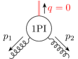
(a)

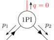
(b)

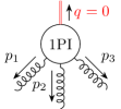
(c)

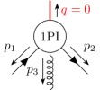
(d)

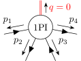
(e)

Figure 2: 1PI graphs considered to perform the 1-loop renormalisation of the minimal operator basis at zero momentum. The double line indicates the operator insertion at zero momentum. Graph 2(e) is only needed to renormalise the 4-fermion opreators, while the graphs 2(a) and 2(c) would suffice for the case of pure gauge theory.

3.1 Renormalisation strategy

Our strategy to compute the 1-loop anomalous dimensions is based on the background field gauge [17, 18, 19, 20] in which we compute the one-particle-irreducible (1PI) graphs as depicted in fig. 2. This particular choice allows us to easily perform the renormalisation of the inserted operator at zero momentum, which then allows us to ignore any mixing from total divergence operators. Since we perform our operator renormalisation off-shell we have to take EOM vanishing operators $\mathcal{E}$ into account, i.e. the desired mixing matrix $Z^{\mathcal{O}}$ can be extracted from

$$\begin{pmatrix}\mathcal{O}_{i}\\[6.0pt] \mathcal{E}_{j}\end{pmatrix}_{\overline{\text{MS}}}=\begin{pmatrix}Z_{ik}^{\mathcal{O}}&Z^{\mathcal{O}\mathcal{E}}_{il}\\[6.0pt] 0&Z^{\mathcal{E}}_{jl}\end{pmatrix}\begin{pmatrix}\mathcal{O}_{k}\\[6.0pt] \mathcal{E}_{l}\end{pmatrix},$$ (7)

where the subscript $\overline{\text{MS}}$ indicates that we are using the $\overline{\text{MS}}$ renormalisation scheme working in $D=4-2\epsilon$ dimensions. The 1-loop coefficient of the anomalous dimension matrix can then be easily obtained from the mixing matrix

$$Z^{\mathcal{O}}=\mathbb{1}+\gamma_{0}^{\mathcal{O}}\frac{\bar{g}^{2}}{\epsilon}+\mathrm{O}(\bar{g}^{4}).$$ (8)

3.2 Leading powers $\hat{\Gamma}_{j}$

Following the strategy described before, we are left with a range of values $\hat{\Gamma}_{j}$ and the (unknown) constants $d_{j}=\hat{c}_{j}^{\mathcal{B}}\delta\mathcal{P}_{j;\mathrm{RGI}}^{\mathcal{B}}$. If a matching coefficient $c_{j}^{\mathcal{B}}$ vanishes at tree-level, we assume the 1-loop order to be the first non-vanishing contribution – of course those contributions could still be further suppressed. For an in-depth discussion of $\hat{c}_{j}^{\mathcal{B}}$ for commonly used lattice discretisations, see [16]. We will rather focus here on the spectrum $\hat{\Gamma}_{j}$ and try to make statements about the leading lattice artifacts ignoring potential hierarchies between different $\hat{c}_{j}^{\mathcal{B}}$. The plots in figure 3 show all powers $\hat{\Gamma}_{j}$ for $\mathrm{O}(a)$ improved Wilson and GW quarks respectively up to N³LO contributions. This is done to indicate the large spread of $\hat{\Gamma}_{j}$ at leading order, while anything beyond $\hat{\Gamma}_{j}\leq 1+\min_{i}\hat{\Gamma}_{i}$ will be hard to distinguish from e.g. the NLO contributions of the truly leading powers. Also the very dense spectrum at subleading orders becomes more apparent this way.

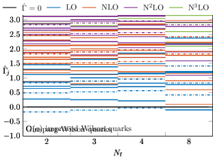
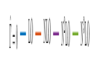
Figure 3: Spectra of $\hat{\Gamma}_{j}$ for Wilson (left) and Ginsparg-Wilson quarks (right). All powers up to N³LO have been plotted to highlight the spread of the leading powers and the density at subleading powers. While the solid lines correspond to the contributions from the massless operator basis in eq. (2), the dash-dotted lines correspond to contributions from massive operators. The number of flavours is chosen as $N_{\mathrm{f}}=2,3,4$ for the conventional lattice simulations and as $N_{\mathrm{f}}=8$ to highlight the approach to the conformal window. Notice that due to the dense spectrum some contributions are hard to distinguish.

4 Conclusion

We find a very dense spectrum $\hat{\Gamma}_{j}$ for both Wilson and GW quarks due to the presence of four fermion operators at mass-dimension 6. This will make it hard to decide, which contributions actually dominate the $\mathrm{O}(a^{2})$ lattice artifacts due to potentially complicated cancellations and pile-ups of the various contributions. Nonetheless, ignoring any hierarchy between the matching coefficients, we find e.g. for $N_{\mathrm{f}}=3$ the leading asymptotic dependence for spectral quantities (ordering $\hat{\Gamma}_{i}\leq\hat{\Gamma}_{i+1}$)

$$\frac{\mathcal{P}(a)}{\mathcal{P}(0)}=1-a^{2}[2b_{0}\bar{g}^{2}(1/a)]^{\hat{\Gamma}_{\mathrm{min}}}\left\{d_{1}+d_{2}[2b_{0}\bar{g}^{2}(1/a)]^{\Delta\hat{\Gamma}}+\ldots\right\},\quad\begin{tabular}[]{lrr}&massless&massive\\ $\hat{\Gamma}_{\mathrm{min}}$&$0.25$&$-0.11$\\ $\Delta\hat{\Gamma}$&$0.42$&$0.36$\end{tabular},$$ (9)

which is universal for $\mathrm{O}(a)$ improved Wilson and Ginsparg-Wilson quarks. The asymptotic form for the massless case should also be a good approximation for $N_{\mathrm{f}}=2$ and may still work at $N_{\mathrm{f}}=2+1$ at physical quark masses. Once the physical charm quark is added the contributions from massive operators will certainly not be small any longer and may actually be the dominant contributions.

For the massless case and $N_{\mathrm{f}}=2,3,4$ the convergence towards the continuum limit should be slightly improved due to $\hat{\Gamma}_{i}>0$, while both $N_{\mathrm{f}}=8$ and the massive case have slightly negative $\hat{\Gamma}_{i}\gtrsim-0.2$, such that the convergence might be worse. In contrast to the O(3) non-linear sigma model [6, 7] all leading powers are very close to the classical zero and not distinctly negative, i.e. $\hat{\Gamma}_{i}\gg-3$, which is good news.

When the different constants $d_{j}$ have a similar magnitude, the leading power in the coupling dominates the $a^{2}$ effects. However, as analysed in some detail in [16], common lattice actions can have $\hat{c}_{j}^{\mathcal{B}}$ which differ very much. For example for an $\mathrm{O}(a)$ improved fermion action and an improved gauge action, a single term dominates and it does not have the leading power. Such information should be incorporated when continuum extrapolations are performed and checks on contaminations of $\mathrm{O}(a^{3})$ or $\mathrm{O}(a^{4})$ contributions are advisable as well. Necessary extensions to this work are amongst others the inclusion of contributions from local fields to go beyond spectral quantities and staggered quarks, which require an enlarged operator basis due to flavour changing interactions.

Acknowledgements: We thank Hubert Simma, Kay Schönwald and Agostino Patella for useful discussions and suggestions. RS acknowledges funding by the H2020 program in the Europlex training network, grant agreement No. 813942.

References

- [1] T. Luthe, A. Maier, P. Marquard and Y. Schröder, Complete renormalization of QCD at five loops, JHEP 03 (2017) 020 [1701.07068].
- [2] K. Symanzik, Cutoff dependence in lattice theory, NATO Sci. Ser. B 59 (1980) 313.
- [3] K. Symanzik, Some Topics in Quantum Field Theory, in Mathematical Problems in Theoretical Physics. Proceedings, 6th International Conference on Mathematical Physics, West Berlin, Germany, August 11-20, 1981, pp. 47–58, 1981.
- [4] K. Symanzik, Continuum Limit and Improved Action in Lattice Theories. 1. Principles and Theory, Nucl. Phys. B226 (1983) 187.
- [5] K. Symanzik, Continuum Limit and Improved Action in Lattice Theories. 2. O(N) Nonlinear Sigma Model in Perturbation Theory, Nucl. Phys. B226 (1983) 205.
- [6] J. Balog, F. Niedermayer and P. Weisz, Logarithmic corrections to O() lattice artifacts, Phys. Lett. B676 (2009) 188 [0901.4033].
- [7] J. Balog, F. Niedermayer and P. Weisz, The Puzzle of apparent linear lattice artifacts in the 2d non-linear sigma-model and Symanzik’s solution, Nucl. Phys. B824 (2010) 563 [0905.1730].
- [8] N. Husung, P. Marquard, R. Sommer, Asymptotic behavior of cutoff effects in Yang-Mills theory and in Wilson’s lattice QCD, Eur. Phys. J. C 80 (2020) 200 [1912.08498].
- [9] K. G. Wilson, Confinement of quarks, Phys. Rev. D 10 (1974) 2445.
- [10] K. G. Wilson, Quarks and Strings on a Lattice, in New Phenomena in Subnuclear Physics: Proceedings, International School of Subnuclear Physics, Erice, Sicily, Jul 11-Aug 1 1975. Part A, p. 99, 1975.
- [11] M. Lüscher, S. Sint, R. Sommer and P. Weisz, Chiral symmetry and O(a) improvement in lattice QCD, Nucl. Phys. B478 (1996) 365 [hep-lat/9605038].
- [12] P. Weisz, Continuum Limit Improved Lattice Action for Pure Yang-Mills Theory (I), Nucl. Phys. B212 (1983) 1.
- [13] M. Lüscher and P. Weisz, On-Shell Improved Lattice Gauge Theories, Commun. Math. Phys. 97 (1985) 59.
- [14] B. Sheikholeslami and R. Wohlert, Improved Continuum Limit Lattice Action for QCD with Wilson Fermions, Nucl. Phys. B259 (1985) 572.
- [15] N. Husung, Logarithmic corrections to O() and O() effects in lattice QCD with Wilson or Ginsparg-Wilson quarks, in preperation (2021) .
- [16] N. Husung, P. Marquard and R. Sommer, The asymptotic approach to the continuum of lattice QCD spectral observables, in preperation (2021) [2111.02347].
- [17] G. ’t Hooft, The Background Field Method in Gauge Field Theories, in Functional and Probabilistic Methods in Quantum Field Theory. 1. Proceedings, 12th Winter School of Theoretical Physics, Karpacz, Feb 17-March 2, 1975, pp. 345–369, 1975.
- [18] L. F. Abbott, The Background Field Method Beyond One Loop, Nucl. Phys. B185 (1981) 189.
- [19] L. F. Abbott, Introduction to the Background Field Method, Acta Phys. Polon. B13 (1982) 33.
- [20] M. Lüscher and P. Weisz, Background field technique and renormalization in lattice gauge theory, Nucl. Phys. B452 (1995) 213 [hep-lat/9504006].