Nuclear DFT analysis of electromagnetic moments in odd near doubly magic nuclei

Abstract

We use the nuclear density functional theory to determine nuclear electric quadrupole and magnetic dipole moments in all one-particle and one-hole neighbours of eight doubly magic nuclei. We align angular momenta along the intrinsic axial-symmetry axis with broken time-reversal symmetry, which allows us to explore fully the self-consistent charge, spin, and current polarisation. Spectroscopic moments are determined for symmetry-restored wave functions and compared with available experimental data. We find that the obtained polarisations do not call for using quadrupole- or dipole-moment operators with effective charges or effective $g$-factors.

Nuclear electromagnetic moments provide essential information in our understanding of nuclear structure. Observables such as electric quadrupole moments are highly sensitive to collective nuclear phenomena [1, 2], while magnetic dipole moments offer sensitive probes to test our description of microscopic properties such as those of valence nucleons [3, 4, 5, 6, 7, 8] and the role of nuclear electroweak currents [9, 10]. Although great progress was achieved in the description of electromagnetic properties of light nuclei [10] and experimental trends in certain isotopic chains, a unified and consistent description of nuclear electromagnetic properties remains an open challenge for nuclear theory.

Traditionally, shell model calculations were successful in describing experimental trends of electromagnetic moments [11, 1, 3, 12, 13]. However, these calculations require the use of effective nuclear charges and effective $g$-factors that are most often phenomenologically adjusted to data and sometimes lead to marked disagreements in different regions of the nuclear chart [4, 14, 15, 16]. The nuclear DFT calculations in even-even nuclei have demonstrated a good overall description of nuclear charge radii, see, e.g., Refs. [17, 18, 19, 20] and electric quadrupole moments (in deformed nuclei BE2($2^{+}_{1}\rightarrow 0^{+}_{1}$) transitions) [21, 22] across the nuclear chart. An analogous global DFT description of the magnetic dipole moments [23, 24, 25, 26, 27, 28, 29, 30] has not been fully developed so far.

In this Letter, we employ the nuclear DFT to address the challenge of describing the electric and magnetic moments globally, that is, without adjusting interactions, coupling constants, valence spaces, or effective charges/$g$-factors separately in different regions of the nuclear chart. In particular, our work provides the first global adjustment of nuclear DFT’s time-odd mean-field sector to magnetic dipole moments. To minimize the possible pairing or beyond-mean-field effects, such as, e.g., the coupling to collective motion, we chose to look at the simplest possible cases of one-particle and one-hole neighbours of the doubly magic nuclei. In addition, to check if the data indicate a need for corrective terms, we used the simplest one-body magnetic-moment operator. Here we note that the two-body-current extensions of the Gamow-Teller transition operator were shown to bring important improvement to the agreement with data [9, 31]. Establishing the baseline for including analogous corrections to the magnetic-moment operator is, therefore, of paramount importance. The deformed DFT approach is probably close to a spherical Quasiparticle-Phonon Interaction method [32, 33, 34, 35, 36, 37, 38], with an explicit coupling of spherical quasiparticles and phonons replaced by the use of symmetry-restored deformed DFT configurations. However, a dedicated comparative analysis of prospective links is not available yet.

In nuclear DFT, properties of odd nuclei can be analyzed in terms of the self-consistent polarisation effects caused by the presence of the unpaired nucleon. Indeed, the non-zero quadrupole moment of the odd nucleon induces deformation of the total mean field and thus generates quadrupole moments of all remaining core nucleons. The latter enhance the deformation of the mean field even more, which in turn influences the quadrupole moment of the odd nucleon. In the self-consistent solution, these mutual polarisations are effectively summed up to infinity, whereupon the final total electric quadrupole moment $Q$ is generated [39].

In a similar way, non-zero spin and current distributions of the odd particle influence those of all other nucleons; in the self-consistent solution they lead to a specific polarisation of the system and give the total magnetic dipole moment $\mu$. All nucleons contribute to the total moments, $Q$ and $\mu$, of the system, with their individual contributions depending on polarisation responses to the deformed and polarised mean fields. The broken-symmetry nuclear DFT used here opens up a possibility of studying polarisation effects in full. We note that approaches that start from unpolarised spherical states are bound to treat the polarisation effects perturbatively, see, e.g., Refs. [11, 35, 28]. In this Letter, we show that the inclusion of self-consistent DFT spin and current polarisation effects removes the necessity of introducing an effective spin $g$-factor from the description of nuclear magnetic dipole moments.

In this work, we determined the electric quadrupole moments $Q$ and magnetic dipole moments $\mu$ of 32 nuclei that are one-particle or one-hole neighbours of eight doubly magic nuclei: ¹⁶O, ⁴⁰Ca, ⁴⁸Ca, ⁵⁶Ni, ⁷⁸Ni, ¹⁰⁰Sn, ¹³²Sn, and ²⁰⁸Pb. We employed code hfodd (v3.07h) [40] for three Skyrme functionals, UNEDF1 [41], SLy4 [42], and SkO^′ [43]; for the Gogny functional D1S [44]; and for the regularized functional N³LO (REG6d.190617) [45]. We used the spherical basis of $N_{0}=16$ shells.

We begun our analysis by selecting in doubly magic nuclei the spherical orbitals that were closest to the Fermi energies, that is, the lowest particle or highest hole orbitals were selected in odd-particle or odd-hole nuclei, respectively. As it turned out, this rule gave the same orbitals irrespective of which of the five functionals were considered. In addition, this rule gave orbitals corresponding to the ground-state spins and parities of odd nuclei, whenever they were experimentally known. The exception was the $I=\frac{3}{2}^{+}$ experimental ground state of ¹³¹Sn, whereas the $I=\frac{11}{2}^{-}$ state was used in the present study.

Next, relative to the doubly magic nuclei, configurations of odd-particle (odd-hole) nuclei were fixed by occupying (emptying) deformed substates that originated from a given spherical orbital and had the highest-positive (lowest-negative) value of $\Omega$, where $\Omega$ denotes the eigenvalue of the projection of the single-particle angular-momentum operator on the axial-symmetry axis. The chosen single-particle occupations thus always corresponded to the maximally aligned total angular momenta, $\Omega=+I$. Such occupations yielded the oblate (prolate) self-consistent intrinsic shapes for odd-particle (odd-hole) $I>\frac{1}{2}$ nuclei and vice versa for $I=\frac{1}{2}$. For the configurations defined in this way, fully self-consistent [46, 47] unpaired solutions were obtained for all odd nuclei considered in this work. The convergence was stabilized by fixing specific partitions of occupations among different $\Omega$ blocks, as described in detail in [40].

By occupying specific odd orbitals having good quantum numbers $\Omega$, we aligned the angular momenta of odd unpaired nuclei along the axial-symmetry axis of a deformed nucleus. This choice of occupations requires explicit breaking of the time-reversal symmetry in the intrinsic reference frame. As the direction of alignment with respect to the nuclear shape strongly impacts the spin and current polarisation effects [48], this choice of occupations constitutes an essential element of the DFT approach to magnetic moments [23, 24, 26].

The aligned configurations were strictly axial, which allowed us to determine the angular-momentum-projected states $|IM\rangle$ [49] by employing a one-dimensional integration over the Euler angle $\beta$ only,

$$|IM\rangle=N_{IM}\int_{0}^{\pi}\mathrm{d}\beta\,d^{I}_{M\Omega}(\beta)\exp\big{(}-\mathrm{i}\beta\hat{I}_{y}\bigr{)}|\Omega\rangle,$$ (1)

where $d^{I}_{M\Omega}$ are the Wigner functions [50], $M$ is the projection of the angular momentum on the laboratory $z$-axis, $\hat{I}_{y}$ denotes the $y$-component of the angular-momentum operator, $|\Omega\rangle$ denotes the self-consistent deformed intrinsic state defined above, and $N_{IM}$ is a normalization factor. Instead of relying on approximate relations between the intrinsic and spectroscopic nuclear moments, we determined the standard magnetic $\mu$ and quadrupole $Q$ spectroscopic moments of the angular-momentum-projected states $|IM\rangle$ as [46]

$$\mu=\sqrt{\frac{4\pi}{3}}\langle II|\hat{M}_{10}|II\rangle,\quad Q=\sqrt{\frac{16\pi}{5}}\langle II|\hat{Q}_{20}|II\rangle,$$ (2)

where $\hat{M}_{1\nu}$ and $\hat{Q}_{2\nu}$ are the $\nu$th magnetic components of the corresponding M1 and E2 electromagnetic operators [51], respectively. In this way, we could compare the calculated magnetic and quadrupole moments directly with experimental data.

For the Skyrme functionals, one can separately adjust coupling constants in the time-odd mean-field sector of the functional [52]. The impact of the time-odd mean-field sector of the Skyrme functional on time-even observables (masses, radii, etc.), or single-particle energies or spins and parities of ground states is small, and smaller than overall deviations of these observables from data, see, e.g., [53]. Here we focus on studying the simplest terms in the time-odd mean-field sector, which correspond to the spin-spin interactions $\bm{\sigma}_{1}\cdot\bm{\sigma}_{2}$. Following [54], we parametrize these terms by the standard isoscalar and isovector Landau parameters $g_{0}$ and $g_{0}^{\prime}$, respectively. Since variations of the isoscalar Landau parameter $g_{0}$ do not change the results, we fixed it at $g_{0}=0.4$, which was the value recommended in [54].

An important aspect of this work was to consistently follow given configurations in function of the Landau parameter $g_{0}^{\prime}$. This was possible in all cases but for a few difficult ones encountered for functional SkO^′. In particular, in ¹⁰¹Sn, the converged solutions could not be obtained at any value of $g_{0}^{\prime}$ and in ⁴⁷K at $g_{0}^{\prime}>1.7$. This was caused by a strong mixing with the neighboring deformed substates that had the same values of $\Omega$. In addition, converged solutions obtained in ⁵⁷Ni and ⁵⁷Cu turned out to have unusually large deformations and thus became incomparable to those obtained for the remaining four functionals studied here.

Theoretical uncertainties of the calculated magnetic moments were estimated using the Bayesian Model Averaging (BMA) analysis [55]. In our implementation of the BMA, the unique variable parameter was assumed to be the Landau parameter $g_{0}^{\prime}$, for which, based on Refs. [56, 54], we adopted a Gaussian prior distribution of mean 1.2 and of variance 0.5. Theoretical BMA error bars shown below correspond to the posterior estimates of the uncertainties of the $g_{0}^{\prime}$ optimum values obtained for Skyrme functionals UNEDF1 and SLy4 in ¹⁰¹Sn, ⁴⁷K, ⁵⁷Ni, and ⁵⁷Cu and for Skyrme functionals UNEDF1, SLy4, and SkO^′ in all other nuclei.

Our study combines several aspects of the DFT approach to nuclear moments that were never simultaneously considered so far. For example, previous studies determined the intrinsic and not spectroscopic moments [23, 24, 26, 29, 30], used phenomenological description of the core contributions [25, 28, 29, 30], or neglected time-reversal breaking [27, 29, 30] or deformation [25, 28] in the intrinsic reference frame.

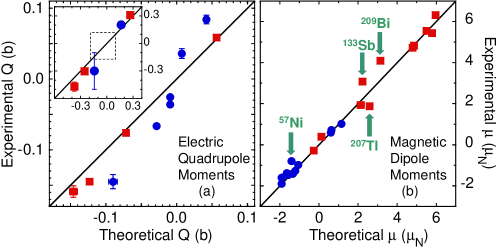
Figure 1: Calculated electric quadrupole moments $Q$, panel (a), compared with 15 experimentally measured values (the inset shows values that are outside the area of the main plot, as visualized by the dashed-line square drawn inside). Panel (b) shows analogous results obtained for the magnetic dipole moments $\mu$ compared with 23 experimentally measured values (the arrows mark the outlier cases discussed in the text). Full circles (squares) show results obtained for $N$-odd ($Z$-odd) nuclei. Calculated values shown in this figure were derived within the Bayesian Model Averaging (BMA) analysis. Apart from one point, the corresponding theoretical error bars are always smaller than the sizes of symbols.

Before presenting details of our results, in figure 1 we show an overview of the comparison with the presently available experimental data. We see that owing to the use of the whole unabridged single-particle phase space, nuclear functionals properly account for the charge and spin polarisations without invoking effective charges or effective $g$-factors.

				Electric quadrupole moment $Q$ (b)
Nuclide	$I^{\pi}$	$[Nn_{z}\Lambda]K$	orbital	EXP	Ref.	UNEDF1	SLy4	SkO′	D1S	N3LO	Average
17O	${\textstyle\frac{5}{2}}^{+}$	[202]5/2	1$d_{5/2}$	$-$0.0256(2)∗	[57]	$-$0.0108	$-$0.0087	$-$0.0086	$-$0.0085	$-$0.0098	$-$0.0093(9)
17F	${\textstyle\frac{5}{2}}^{+}$	[202]5/2	1$d_{5/2}$	$-$0.076(4)∗	[57]	$-$0.0712	$-$0.0721	$-$0.0720	$-$0.0730	$-$0.0691	$-$0.0715(13)
39Ca	${\textstyle\frac{3}{2}}^{+}$	[202]3/2	1$d_{3/2}$	0.036(7)	[57]	0.0075	0.0070	0.0070	0.0073	0.0072	0.0072(2)
41Ca	${\textstyle\frac{7}{2}}^{-}$	[303]7/2	1$f_{7/2}$	$-$0.0665(18)	[57]	$-$0.0323	$-$0.0270	$-$0.0270	$-$0.0263	$-$0.0288	$-$0.028(2)
39K	${\textstyle\frac{3}{2}}^{+}$	[202]3/2	1$d_{3/2}$	0.0585(6)	[57]	0.0546	0.0580	0.0565	0.0576	0.0555	0.0564(13)
41Sc	${\textstyle\frac{7}{2}}^{-}$	[303]7/2	1$f_{7/2}$	$-$0.145(3)∗	[57]	$-$0.1199	$-$0.1255	$-$0.1218	$-$0.1266	$-$0.1211	$-$0.123(3)
47Ca	${\textstyle\frac{7}{2}}^{-}$	[303]7/2	1$f_{7/2}$	0.084(6)	[4]	0.0460	0.0395	0.0441	0.0379	0.0415	0.042(3)
49Ca	${\textstyle\frac{3}{2}}^{-}$	[301]3/2	2$p_{3/2}$	$-$0.036(3)	[4]	$-$0.0104	$-$0.0084	$-$0.0094	$-$0.0079	$-$0.0103	$-$0.0093(10)
49Sc	${\textstyle\frac{7}{2}}^{-}$	[303]7/2	1$f_{7/2}$	$-$0.159(8)	[58]	$-$0.1545	$-$0.1455	$-$0.1496	$-$0.1408	$-$0.1393	$-$0.146(6)
55Ni	${\textstyle\frac{7}{2}}^{-}$	[303]7/2	1$f_{7/2}$			0.1637	0.1486	0.1661	0.1274	0.1336	0.148(16)
57Ni	${\textstyle\frac{3}{2}}^{-}$	[301]3/2	2$p_{3/2}$			$-$0.0685	$-$0.0511	$-$0.1622	$-$0.0434	$-$0.0518	$-$0.054(9)∗∗
55Co	${\textstyle\frac{7}{2}}^{-}$	[303]7/2	1$f_{7/2}$			0.2254	0.2241	0.2371	0.2086	0.2091	0.221(11)
57Cu	${\textstyle\frac{3}{2}}^{-}$	[301]3/2	2$p_{3/2}$			$-$0.1207	$-$0.1143	$-$0.1919	$-$0.1077	$-$0.1096	$-$0.113(5)∗∗
77Ni	${\textstyle\frac{9}{2}}^{+}$	[404]9/2	1$g_{9/2}$			0.1600	0.1305	0.1555	0.1197	0.1275	0.139(16)
79Ni	${\textstyle\frac{5}{2}}^{+}$	[402]5/2	2$d_{5/2}$			$-$0.0797	$-$0.0601	$-$0.0825	$-$0.0513	$-$0.0581	$-$0.066(13)
77Co	${\textstyle\frac{7}{2}}^{-}$	[303]7/2	1$f_{7/2}$			0.2075	0.1847	0.2121	0.1874	0.1778	0.194(13)
79Cu	${\textstyle\frac{3}{2}}^{-}$	[301]3/2	2$p_{3/2}$			$-$0.1033	$-$0.0962	$-$0.0853	$-$0.0940	$-$0.0910	$-$0.094(6)
99Sn	${\textstyle\frac{9}{2}}^{+}$	[404]9/2	1$g_{9/2}$			0.1719	0.1628	0.1773	0.1507	0.1575	0.164(10)
101Sn	${\textstyle\frac{5}{2}}^{+}$	[402]5/2	2$d_{5/2}$			$-$0.0927	$-$0.0842		$-$0.0788	$-$0.0920	$-$0.0870(6)∗∗
99In	${\textstyle\frac{9}{2}}^{+}$	[404]9/2	1$g_{9/2}$			0.2848	0.2935	0.3040	0.2865	0.2848	0.291(7)
101Sb	${\textstyle\frac{7}{2}}^{+}$	[404]7/2	1$g_{7/2}$			$-$0.2936	$-$0.2975	$-$0.2858	$-$0.2921	$-$0.2903	$-$0.292(4)
131Sn	${\textstyle\frac{11}{2}}^{-}$	[505]11/2	1$h_{11/2}$	0.203(4)	[59]	0.1737	0.1616	0.1780	0.1507	0.1596	0.165(10)
133Sn	${\textstyle\frac{7}{2}}^{-}$	[503]7/2	2$f_{7/2}$	$-$0.145(10)	[13]	$-$0.0919	$-$0.0845	$-$0.0979	$-$0.0815	$-$0.0941	$-$0.090(6)
131In	${\textstyle\frac{9}{2}}^{+}$	[404]9/2	1$g_{9/2}$	0.31(1)	[8]	0.2615	0.2664	0.2815	0.2712	0.2589	0.268(8)
133Sb	${\textstyle\frac{7}{2}}^{+}$	[404]7/2	1$g_{7/2}$	$-$0.304(7)	[16]	$-$0.2549	$-$0.2566	$-$0.2503	$-$0.2609	$-$0.2508	$-$0.255(4)
209Pb	${\textstyle\frac{9}{2}}^{+}$	[604]9/2	2$g_{9/2}$	$-$0.27(17)	[57]	$-$0.1514	$-$0.1450	$-$0.1348	$-$0.1325	$-$0.1510	$-$0.143(8)
209Bi	${\textstyle\frac{9}{2}}^{-}$	[505]9/2	1$h_{9/2}$	$-$0.47(5)∗∗∗	[57, 60]	$-$0.3710	$-$0.3736	$-$0.3661	$-$0.3835	$-$0.3643	$-$0.372(7)
∗sign not measured; calculated sign was assigned.
∗∗functional SkO′ excluded.
∗∗∗average of $-$0.516(15) [57] and $-$0.418(6) [60] with the error bar reflecting uncertainties of the atomic
theory.

Table 1: Experimental values of the electric quadrupole moments $Q$ compared with those calculated for functionals UNEDF1, SLy4, SkO^′, D1S, and N³LO.

				Magnetic dipole moment $\mu$ ($\mu_{N}$)
Nuclide	$I^{\pi}$	$[Nn_{z}\Lambda]K$	orbital	EXP	Ref.	UNEDF1	SLy4	SkO′	D1S	N3LO	Average	BMA
15O	${\textstyle\frac{1}{2}}^{-}$	[101]1/2	1$p_{1/2}$	0.71951(12)∗	[61]	0.6366	0.6372	0.6384	0.6369	0.6352	0.6369(10)	0.6375(8)
17O	${\textstyle\frac{5}{2}}^{+}$	[202]5/2	1$d_{5/2}$	$-$1.89379(9)∗	[61]	$-$1.9081	$-$1.9092	$-$1.9090	$-$1.9098	$-$1.9091	$-$1.9090(6)	$-$1.9087(5)
15N	${\textstyle\frac{1}{2}}^{-}$	[101]1/2	1$p_{1/2}$	$-$0.2830569(14)∗	[62]	$-$0.2632	$-$0.2638	$-$0.2651	$-$0.2632	$-$0.2616	$-$0.2634(12)	$-$0.2642(8)
17F	${\textstyle\frac{5}{2}}^{+}$	[202]5/2	1$d_{5/2}$	4.7223(12)∗	[61]	4.7878	4.7890	4.7881	4.7895	4.7889	4.7887(6)	4.7882(6)
39Ca	${\textstyle\frac{3}{2}}^{+}$	[202]3/2	1$d_{3/2}$	1.02168(12)	[61]	1.1465	1.1468	1.1476	1.1472	1.1469	1.1470(4)	1.1470(5)
41Ca	${\textstyle\frac{7}{2}}^{-}$	[303]7/2	1$f_{7/2}$	$-$1.5942(7)	[61]	$-$1.9088	$-$1.9099	$-$1.9098	$-$1.9098	$-$1.9098	$-$1.9096(4)	$-$1.9096(4)
39K	${\textstyle\frac{3}{2}}^{+}$	[202]3/2	1$d_{3/2}$	0.39147(3)	[61]	0.1259	0.1256	0.1249	0.1251	0.1255	0.1254(4)	0.1254(4)
41Sc	${\textstyle\frac{7}{2}}^{-}$	[303]7/2	1$f_{7/2}$	5.431(2)∗	[61]	5.7886	5.7897	5.7888	5.7896	5.7895	5.7892(5)	5.7890(5)
47Ca	${\textstyle\frac{7}{2}}^{-}$	[303]7/2	1$f_{7/2}$	$-$1.4064(11)	[4]	$-$1.4113	$-$1.3232	$-$1.2991	$-$1.4894	$-$1.4248	$-$1.39(7)	$-$1.33(10)
49Ca	${\textstyle\frac{3}{2}}^{-}$	[301]3/2	2$p_{3/2}$	$-$1.3799(8)	[4]	$-$1.6506	$-$1.6494	$-$1.6530	$-$1.7090	$-$1.6607	$-$1.66(2)	$-$1.65(4)
47K	${\textstyle\frac{1}{2}}^{+}$	[220]1/2	2$s_{1/2}$	1.933(9)	[61]	2.2040	2.0786	2.2958	2.4801	2.5769	2.33(18)	2.13(7)∗∗
49Sc	${\textstyle\frac{7}{2}}^{-}$	[303]7/2	1$f_{7/2}$	5.539(4)	[58]	5.3409	5.4636	5.6621	5.6127	5.4734	5.51(11)	5.50(14)
55Ni	${\textstyle\frac{7}{2}}^{-}$	[303]7/2	1$f_{7/2}$	$-$0.98(3)∗	[63]	$-$1.1009	$-$1.0923	$-$1.0309	$-$1.3596	$-$1.1638	$-$1.15(11)	$-$1.06(13)
57Ni	${\textstyle\frac{3}{2}}^{-}$	[301]3/2	2$p_{3/2}$	$-$0.7975(14)∗	[61]	$-$1.3267	$-$1.4371	$-$0.4178	$-$1.5227	$-$1.4261	$-$1.43(7)∗∗	$-$1.40(8)∗∗
55Co	${\textstyle\frac{7}{2}}^{-}$	[303]7/2	1$f_{7/2}$	4.822(3)∗	[61]	4.9296	4.8991	4.8016	5.1811	4.9969	4.96(13)	4.86(15)
57Cu	${\textstyle\frac{3}{2}}^{-}$	[301]3/2	2$p_{3/2}$			3.1759	3.2968	2.0319	3.4081	3.2944	3.29(8)∗∗	3.26(8)∗∗
77Ni	${\textstyle\frac{9}{2}}^{+}$	[404]9/2	1$g_{9/2}$			$-$1.2069	$-$1.1768	$-$1.1414	$-$1.4322	$-$1.2563	$-$1.24(10)	$-$1.16(13)
79Ni	${\textstyle\frac{5}{2}}^{+}$	[402]5/2	2$d_{5/2}$			$-$1.5128	$-$1.5542	$-$1.4924	$-$1.6529	$-$1.5754	$-$1.56(6)	$-$1.51(8)
77Co	${\textstyle\frac{7}{2}}^{-}$	[303]7/2	1$f_{7/2}$			4.9185	4.9234	4.7569	5.1730	4.9936	4.95(13)	4.85(16)
79Cu	${\textstyle\frac{3}{2}}^{-}$	[301]3/2	2$p_{3/2}$			3.2102	3.3391	3.3742	3.4565	3.3927	3.35(8)	3.31(8)
99Sn	${\textstyle\frac{9}{2}}^{+}$	[404]9/2	1$g_{9/2}$			$-$1.2018	$-$1.1918	$-$1.1477	$-$1.4448	$-$1.2608	$-$1.25(10)	$-$1.17(13)
101Sn	${\textstyle\frac{5}{2}}^{+}$	[402]5/2	2$d_{5/2}$			$-$1.4674	$-$1.4968		$-$1.5824	$-$1.4956	$-$1.51(4)∗∗	$-$1.50(8)∗∗
99In	${\textstyle\frac{9}{2}}^{+}$	[404]9/2	1$g_{9/2}$			6.0398	6.0097	5.9342	6.2765	6.1021	6.07(12)	5.98(14)
101Sb	${\textstyle\frac{7}{2}}^{+}$	[404]7/2	1$g_{7/2}$			2.2721	2.1716	2.1604	2.1313	2.1465	2.18(5)	2.20(8)
131Sn	${\textstyle\frac{11}{2}}^{-}$	[505]11/2	1$h_{11/2}$	$-$1.267(1)	[59]	$-$1.2443	$-$1.2301	$-$1.2174	$-$1.4868	$-$1.3184	$-$1.30(10)	$-$1.22(13)
133Sn	${\textstyle\frac{7}{2}}^{-}$	[503]7/2	2$f_{7/2}$	$-$1.410(1)	[13]	$-$1.5391	$-$1.5607	$-$1.5775	$-$1.6580	$-$1.5713	$-$1.58(4)	$-$1.55(8)
131In	${\textstyle\frac{9}{2}}^{+}$	[404]9/2	1$g_{9/2}$	6.312(14)	[8]	6.0340	6.0133	5.9055	6.2650	6.0926	6.06(12)	5.97(15)
133Sb	${\textstyle\frac{7}{2}}^{+}$	[404]7/2	1$g_{7/2}$	3.070(2)	[16]	2.2813	2.1792	2.2088	2.1125	2.1379	2.18(6)	2.23(9)
207Pb	${\textstyle\frac{1}{2}}^{-}$	[501]1/2	3$p_{1/2}$	0.5906(4)	[64]	0.6059	0.6021	0.6129	0.6120	0.5972	0.606(6)	0.606(11)
209Pb	${\textstyle\frac{9}{2}}^{+}$	[604]9/2	2$g_{9/2}$	$-$1.4735(16)	[61]	$-$1.5270	$-$1.5539	$-$1.6222	$-$1.6556	$-$1.5664	$-$1.59(5)	$-$1.56(9)
207Tl	${\textstyle\frac{1}{2}}^{+}$	[400]1/2	3$s_{1/2}$	1.876(5)	[61]	2.5797	2.6036	2.6051	2.6475	2.6135	2.61(2)	2.59(4)
209Bi	${\textstyle\frac{9}{2}}^{-}$	[505]9/2	1$h_{9/2}$	4.092(2)	[65]	3.2065	3.1027	3.1249	3.0136	3.0522	3.10(7)	3.15(9)
∗sign not measured; calculated sign was assigned.
∗∗functional SkO′ excluded.

Table 2: Same as in Table 1 but for the magnetic dipole moments $\mu$.

In Tables 1 and 2, we collected all results obtained for electric quadrupole and magnetic dipole moments, respectively. There we also show Nilsson labels and orbitals corresponding to the configurations used, experimental data along with the corresponding references to the original publications or compilations thereof, and averages and RMS deviations of results obtained for the five functionals used in this study. In Table 2, we also show results obtained within the BMA analysis.

As indicated above, we used the standard single-particle magnetic-dipole-moment operator,

$$\hat{\bm{\mu}}\equiv\hat{\bm{M}}_{1}=g_{\ell}^{p}\hat{\bm{L}}_{p}+g_{s}^{n}\hat{\bm{S}}_{n}+g_{s}^{p}\hat{\bm{S}}_{p},$$ (3)

where $\hat{\bm{L}}_{p}$ is the proton orbital angular-momentum operator and $\hat{\bm{S}}_{p}$ ($\hat{\bm{S}}_{n}$) is the proton (neutron) spin operator, and where the bare proton and neutron orbital and spin gyromagnetic factors read

$$g_{\ell}^{p}=\mu_{N},~{}g_{s}^{n}=-3.826\,\mu_{N},~{}g_{s}^{p}=+5.586\,\mu_{N}.$$ (4)

Since the total angular momentum $\hat{\bm{I}}=\sum_{\nu=n,p}(\hat{\bm{L}}_{\nu}+\hat{\bm{S}}_{\nu})$ is conserved, it is convenient to subtract $I\,\mu_{N}$ from the spectroscopic magnetic dipole moments of odd-$Z$ nuclei while leaving those of odd-$N$ nuclei unchanged. In this way, we define the "spin" magnetic dipole moments as

$$\mu^{\mbox{\scriptsize{S}}}_{\mbox{\scriptsize{odd-$Z$}}} \equiv \langle\hat{\bm{\mu}}\rangle-I\,\mu_{N}=g_{\ell}^{n\prime}\langle\hat{\bm{L}}_{n}\rangle+g_{s}^{n\prime}\langle\hat{\bm{S}}_{n}\rangle+g_{s}^{p\prime}\langle\hat{\bm{S}}_{p}\rangle,$$ (5)

$$\mu^{\mbox{\scriptsize{S}}}_{\mbox{\scriptsize{odd-$N$}}} \equiv \langle\hat{\bm{\mu}}\rangle\hskip 32.72066pt=g_{\ell}^{p}\langle\hat{\bm{L}}_{p}\rangle+g_{s}^{n}\langle\hat{\bm{S}}_{n}\rangle+g_{s}^{p}\langle\hat{\bm{S}}_{p}\rangle,$$ (6)

where symbols $\langle\rangle$ denote the standard matrix elements that define spectroscopic moments (2), and

$$g_{\ell}^{n\prime}=-\mu_{N},~{}g_{s}^{n\prime}=-4.826\,\mu_{N},~{}g_{s}^{p\prime}=+4.586\,\mu_{N}.$$ (7)

The spin magnetic dipole moments $\mu^{\mbox{\scriptsize{S}}}$ (5)–(6) can be trivially evaluated for experimental and theoretical results. They allow for comparing odd-$N$ and odd-$Z$ nuclei on an equal footing and in the same scale. Moreover, values of $\mu^{\mbox{\scriptsize{S}}}$ obey a simple rule that defines their signs, namely, those for an odd proton in a $j=\ell+{\textstyle\frac{1}{2}}$ configuration or for an odd neutron in a $j=\ell-{\textstyle\frac{1}{2}}$ configuration are positive and otherwise, they are negative. Therefore, without any loss of information, we can meaningfully plot and compare the absolute values $|\mu^{\mbox{\scriptsize{S}}}|$ only. In this way, by plotting $|\mu^{\mbox{\scriptsize{S}}}|$ in figure 2 we can show and discuss our results in a much finer scale than that used in the overview figure 1(b).

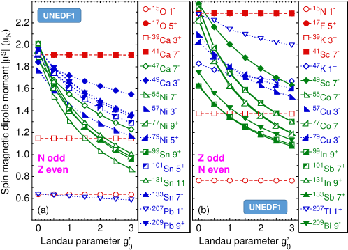
Figure 2: Absolute values of the UNEDF1 spin magnetic dipole moments $|\mu^{\mbox{\scriptsize{S}}}$|, Eqs. (5)–(6), calculated in function of the Landau parameter $g_{0}^{\prime}$ for $N$-odd-$Z$-even (a) and $Z$-odd-$N$-even (b) nuclei. Dashed, solid, and dotted lines denote nuclei belonging to the first, second, and third group discussed in the text, respectively. Values obtained for ¹⁷O and ¹⁷F are hidden behind those obtained for ⁴¹Ca and ⁴¹Sc, respectively. Doubled ground-state spin and parity are given in the legends. Full and empty symbols denote particle and hole states, respectively.

Figure 3: The UNEDF1 magnetic dipole moments $\mu$ calculated in function of the Landau parameter $g_{0}^{\prime}$ relative to the experimental values. Panels (a) and (b) show results that do and do not cross the line of $\mu_{\mbox{\scriptsize{the}}}=\mu_{\mbox{\scriptsize{exp}}}$, respectively. Solid and dotted lines denote nuclei belonging to the second and third group discussed in the text, respectively. Symbols $\times 1/3$ denote outlier values multiplied by a factor of 1/3 to fit in the scale of the figure.

The main thrust of our study is in the dependence of the results on the isovector Landau parameter $g_{0}^{\prime}$. This is what we show in figures 2 and 3 for the UNEDF1 spin magnetic dipole moments $|\mu^{\mbox{\scriptsize{S}}}|$ and residuals $\mu_{\mbox{\scriptsize{the}}}-\mu_{\mbox{\scriptsize{exp}}}$, respectively. The magnetic dipole moments obtained for the 32 nuclei considered in this study allow for grouping them into three distinct sets that illustrate the mechanism of the spin polarisation induced by the isovector spin-spin interaction.

The first group (dashed lines in figure 2) contains eight lightest nuclei around ¹⁶O and ⁴⁰Ca, which are characterized by all spin-orbit partners located on the same side of the Fermi energy. In these nuclei, irrespective of whether an odd proton or an odd neutron, or a hole or particle state, or a high or low spin state are occupied, no tangible polarisation of the spin distribution is obtained and no ensuing dependence of the magnetic dipole moment on the isovector spin-spin interaction is visible. As a result, in this group, all magnetic dipole moments stay quite rigidly fixed at the Schmidt limits [66]. Corrections to the Schmidt values were already studied, see, e.g., [67], with a moderate level of success in describing the experimental data.

The second group (solid lines in figures 2 and 3) contains nuclei around heavier doubly magic nuclei, which are characterized by the Fermi energies separating pairs of the spin-orbit partners from one another, and by a hole or a particle created in one of the spin-orbit partners. In all such nuclei, irrespective of whether the nucleus contains an odd-proton or an odd-neutron, the dependence of the magnetic dipole moments on the isovector spin-spin interaction is strong. Two exceptions from this rule are the cases of ⁴⁷Ca and ⁴⁹Sc, where only the neutron pair of spin-orbit partners is available for polarisation and the response to the isovector spin-spin interaction is somewhat weaker. With increasing values of $g_{0}^{\prime}$, the calculated magnetic dipole moments significantly depart from the Schmidt limits.

The third group (dotted lines in figures 2 and 3) contains nuclei in which particles or holes are created in non-intruder states or their partners. Then, the spin polarisation of the spin-orbit partners becomes weaker and, as a result, the dependence of the magnetic dipole moments on the isovector spin-spin interaction weakens too. For ${\textstyle\frac{1}{2}}^{\pm}$ states, such dependence is particularly weak.

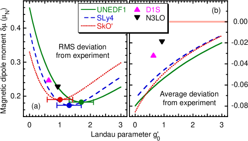
Figure 4: RMS (a) and average (b) deviations $\delta\mu$ between the calculated and experimental values of magnetic dipole moments.

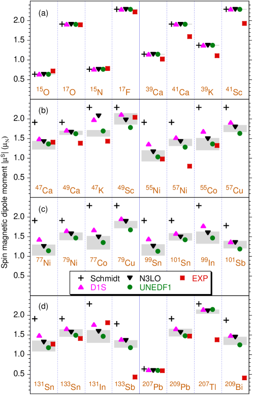
Figure 5: Absolute values of the spin magnetic dipole moments $|\mu^{\mbox{\scriptsize{S}}}|$, Eqs. (5)–(6), calculated for the D1S, N³LO, and UNEDF1 functionals and compared with the Schmidt values and experimental data.

In figures 3(a) and 3(b), we show nuclei whose magnetic dipole moments as functions of $g_{0}^{\prime}$ can and cannot, respectively, be brought down to experimental data. In particular, ⁵⁷Ni, ¹³³Sb, ²⁰⁷Tl, and ²⁰⁹Bi are clear outliers, with the calculated magnetic dipole moments strongly deviating from experiment, see discussion below.

For the other two Skyrme functionals considered in this work, SLy4 and SkO^′, the pattern of dependence of the magnetic dipole moments on the Landau parameter $g_{0}^{\prime}$ is fairly similar. The optimum values of the Landau parameter $g_{0}^{\prime}$, for which the RMS deviations between the calculated and measured magnetic dipole moments are smallest, see the full dots in figure 4(a), are equal to $g_{0}^{\prime}=1.0$, 1.3, and 1.7 for SkO^′, SLy4, and UNEDF1, respectively. Below we present results calculated at these particular values of $g_{0}^{\prime}$. It is rewarding to see that within the estimated uncertainties, the optimum values are not only compatible with one another but also with the estimate derived in Refs. [56, 54] from the analysis of the Gamow-Teller resonances and $\beta$ decays.

In figure 5 we show the complete set of our magnetic dipole moments calculated for the D1S, N³LO, and UNEDF1 functionals and compared with the Schmidt values and experimental data. The shaded bands displayed in the figure correspond to the averages and $1\sigma$ deviations computed within the BMA for the three considered Skyrme functionals.

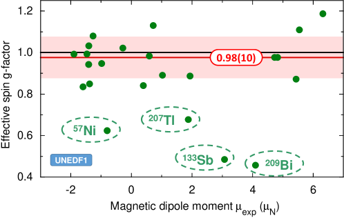
Figure 6: Effective spin $g$-factors $g_{\mbox{\scriptsize{eff}}}$, Eq. (8), that would have been needed for bringing the calculated UNEDF1 magnetic dipole moments $\mu$ to the 23 experimentally measured values.

As one can see in figures 4 and 5, the non-local functionals D1S and N3LO, which have not been explicitly adjusted to time-odd observables, are characterized by somewhat lower values of the Landau parameter $g_{0}^{\prime}$ [68] and deliver values of the magnetic moments in between of those for UNEDF1 and Schmidt values, most often away from data. This calls for performing such adjustments of novel non-local functionals, even though parameters thereof cannot be explicitly separated into two distinct classes characterizing the time-even and time-odd mean-field sectors.

In many theoretical approaches determining nuclear magnetic dipole moments $\mu$ so far, the bare spin gyromagnetic factors of Eq. (4) were multiplied by the so-called effective spin $g$-factor $g_{\mbox{\scriptsize{eff}}}$, that is,

$$g_{s}^{n}=-3.826\,\mu_{N}\times g_{\mbox{\scriptsize{eff}}},\quad~{}g_{s}^{p}=+5.586\,\mu_{N}\times g_{\mbox{\scriptsize{eff}}}.$$ (8)

The DFT results obtained in this work do not support the necessity of using an effective spin $g$-factor for the description of nuclear magnetic dipole moments. Indeed, in figure 6 we show values of $g_{\mbox{\scriptsize{eff}}}$ that would have been needed for bringing the calculated UNEDF1 magnetic dipole moments to measured values. One can clearly see that the average value of $\bar{g}_{\mbox{\scriptsize{eff}}}=0.98(10)$, determined without the outlier cases identified in figures 1(b) and 3(b), is compatible with $g_{\mbox{\scriptsize{eff}}}=1$ and within $\pm 20\%$ covers all results.

Very small outlier values of $g_{\mbox{\scriptsize{eff}}}\leq 0.7$ rather call for a specific configuration-mixing explanation (as already noted long ago [69, 70] and widely discussed thereafter) than for a global modification of the single-particle magnetic-moment operator. We note here that deformed and polarised DFT states automatically include admixtures of large classes of states that in the spherical symmetry must be added explicitly. Nevertheless, mixing of different deformed and polarised DFT configurations [71] is an option that still needs to be considered.

In conclusion, we showed that the nuclear DFT provides a correct global description of nuclear electric quadrupole and magnetic dipole moments in one-particle and one-hole neighbours of doubly magic nuclei. A fair agreement of calculated magnetic dipole moments with data was achieved by adjusting one coupling constant in the time-odd mean-field sector of the nuclear functional. An essential element of the agreement is the self-consistent spin and current polarisation, operating in a whole single-particle phase space, which induces correct dipole moments for bare spin gyromagnetic factors. Our study indicates that the use of effective $g$-factors in previous DFT approaches [26, 29, 30] may be unjustified and that the studies neglecting the time-odd mean fields [27, 29, 30] may be missing an important element of the description. The effective $g$-factors, commonly used in the valence-space approaches, like the shell model, can probably be attributed to the missing single-particle phase space. For the quadrupole moments, the analogous role played by the effective charges has been known since long [39]; here we demonstrated it for the magnetic moments.

Our results provide a baseline for more extensive adjustments in the poorly-known time-odd mean-field sector. Such adjustments may further reduce the scatter of calculated magnetic dipole moments around the experimental values. This, in turn, may be the starting point for the DFT deformed-configuration interaction calculations, especially regarding large outlier deviations of the magnetic dipole moments currently obtained in ⁵⁷Ni, ²⁰⁷Tl, ¹³³Sb, and ²⁰⁹Bi.

Prospective global DFT adjustments and deformed-configuration interaction would open up the possibility of quantifying the roles played by the meson-exchange and/or two-body currents in redefining the magnetic-moment operator. These are of marked importance for the interpretation of modern high-precision experiments such as neutrino physics [31] or dark matter searches [72]. Future measurements of electromagnetic moments of isotopes around doubly magic nuclei will be important to test our theoretical predictions and further constrain DFT developments.

Critical reading of the manuscript by Mike Bentley is gratefully acknowledged. This work was partially supported by the STFC Grant Nos. ST/M006433/1 and ST/P003885/1, by the Polish National Science Centre under Contract No. 2018/31/B/ST2/02220, and by the U.S. Department of Energy, Office of Science, Office of Nuclear Physics under award numbers DE-SC0021176 and DE-SC0021179. We acknowledge the CSC-IT Center for Science Ltd., Finland, for the allocation of computational resources. This project was partly undertaken on the Viking Cluster, which is a high performance compute facility provided by the University of York. We are grateful for computational support from the University of York High Performance Computing service, Viking and the Research Computing team.

References

References

- [1] Neyens G 2003 Reports on Progress in Physics 66 633–689 URL https://doi.org/10.1088/0034-4885/66/4/205
- [2] Babcock C, Heylen H, Bissell M L, Blaum K, Campbell P, Cheal B, Fedorov D, Garcia Ruiz R F, Geithner W, Gins W, Day Goodacre T, Grob L K, Kowalska M, Lenzi S M, Maass B, Malbrunot-Ettenauer S, Marsh B, Neugart R, Neyens G, Nörtershäuser W, Otsuka T, Rossel R, Rothe S, Sánchez R, Tsunoda Y, Wraith C, Xie L and Yang X F 2016 Physics Letters B 760 387–392 ISSN 0370-2693 URL https://www.sciencedirect.com/science/article/pii/S0370269316303574
- [3] Papuga J, Bissell M L, Kreim K, Blaum K, Brown B A, De Rydt M, Garcia Ruiz R F, Heylen H, Kowalska M, Neugart R, Neyens G, Nörtershäuser W, Otsuka T, Rajabali M M, Sánchez R, Utsuno Y and Yordanov D T 2013 Phys. Rev. Lett. 110(17) 172503 URL https://link.aps.org/doi/10.1103/PhysRevLett.110.172503
- [4] Garcia Ruiz R F, Bissell M L, Blaum K, Frömmgen N, Hammen M, Holt J D, Kowalska M, Kreim K, Menéndez J, Neugart R, Neyens G, Nörtershäuser W, Nowacki F, Papuga J, Poves A, Schwenk A, Simonis J and Yordanov D T 2015 Phys. Rev. C 91(4) 041304 URL https://link.aps.org/doi/10.1103/PhysRevC.91.041304
- [5] McCormick B P, Stuchbery A E, Brown B A, Georgiev G, Coombes B J, Gray T J, Gerathy M S M, Lane G J, Kibédi T, Mitchell A J, Reed M W, Akber A, Bignell L J, Dowie J T H, Eriksen T K, Hota S, Palalani N and Tornyi T 2019 Phys. Rev. C 100(4) 044317 URL https://link.aps.org/doi/10.1103/PhysRevC.100.044317
- [6] Boulay F, Simpson G S, Ichikawa Y, Kisyov S, Bucurescu D, Takamine A, Ahn D S, Asahi K, Baba H, Balabanski D L, Egami T, Fujita T, Fukuda N, Funayama C, Furukawa T, Georgiev G, Gladkov A, Hass M, Imamura K, Inabe N, Ishibashi Y, Kawaguchi T, Kawamura T, Kim W, Kobayashi Y, Kojima S, Kusoglu A, Lozeva R, Momiyama S, Mukul I, Niikura M, Nishibata H, Nishizaka T, Odahara A, Ohtomo Y, Ralet D, Sato T, Shimizu Y, Sumikama T, Suzuki H, Takeda H, Tao L C, Togano Y, Tominaga D, Ueno H, Yamazaki H, Yang X F and Daugas J M 2020 Phys. Rev. Lett. 124(11) 112501 URL https://link.aps.org/doi/10.1103/PhysRevLett.124.112501
- [7] Daugas J M, Rosse B, Balabanski D L, Bucurescu D, Kisyov S, Regan P H, Georgiev G, Gaudefroy L, Gladnishki K, Méot V, Morel P, Pietri S, Roig O and Simpson G S 2021 Phys. Rev. C 104(2) 024321 URL https://link.aps.org/doi/10.1103/PhysRevC.104.024321
- [8] Vernon A R, Garcia Ruiz R F, Miyagi T, Binnersley C L, Billowes J, Bissell M L, Bonnard J, Cocolios T E, Dobaczewski J, Farooq-Smith G J, Flanagan K T, Georgiev G, Gins W, de Groote R P, Heinke R, Holt J D, Hustings J, Koszorús Á, Leimbach D, Lynch K M, Neyens G, Stroberg S R, Wilkins S G, Yang X F and Yordanov D T 2022 Nature 607 260 URL https://doi.org/10.1038/s41586-022-04818-7
- [9] Pastore S, Pieper S C, Schiavilla R and Wiringa R B 2013 Phys. Rev. C 87(3) 035503 URL https://link.aps.org/doi/10.1103/PhysRevC.87.035503
- [10] Carlson J, Gandolfi S, Pederiva F, Pieper S C, Schiavilla R, Schmidt K E and Wiringa R B 2015 Rev. Mod. Phys. 87(3) 1067–1118 URL https://link.aps.org/doi/10.1103/RevModPhys.87.1067
- [11] Castel B and Towner I S 1990 Modern theories of nuclear moments (Oxford Studies in Nuclear Physics vol 12) (Clarendon Press) URL https://global.oup.com/academic/product/modern-theories-of-nuclear-moments-9780198517283
- [12] Klose A, Minamisono K, Miller A J, Brown B A, Garand D, Holt J D, Lantis J D, Liu Y, Maaß B, Nörtershäuser W, Pineda S V, Rossi D M, Schwenk A, Sommer F, Sumithrarachchi C, Teigelhöfer A and Watkins J 2019 Phys. Rev. C 99(6) 061301 URL https://link.aps.org/doi/10.1103/PhysRevC.99.061301
- [13] Rodríguez L V, Balabanski D L, Bissell M L, Blaum K, Cheal B, De Gregorio G, Ekman J, Garcia Ruiz R F, Gargano A, Georgiev G, Gins W, Gorges C, Heylen H, Kanellakopoulos A, Kaufmann S, Lagaki V, Lechner S, Maaß B, Malbrunot-Ettenauer S, Neugart R, Neyens G, Nörtershäuser W, Sailer S, Sánchez R, Schmidt S, Wehner L, Wraith C, Xie L, Xu Z Y, Yang X F and Yordanov D T 2020 Phys. Rev. C 102(5) 051301 URL https://link.aps.org/doi/10.1103/PhysRevC.102.051301
- [14] de Groote R P, Billowes J, Binnersley C L, Bissell M L, Cocolios T E, Day Goodacre T, Farooq-Smith G J, Fedorov D V, Flanagan K T, Franchoo S, Garcia Ruiz R F, Koszorús A, Lynch K M, Neyens G, Nowacki F, Otsuka T, Rothe S, Stroke H H, Tsunoda Y, Vernon A R, Wendt K D A, Wilkins S G, Xu Z Y and Yang X F 2017 Phys. Rev. C 96(4) 041302 URL https://link.aps.org/doi/10.1103/PhysRevC.96.041302
- [15] Radhi R A, Alzubadi A A and Ali A H 2018 Phys. Rev. C 97(6) 064312 URL https://link.aps.org/doi/10.1103/PhysRevC.97.064312
- [16] Lechner S, Xu Z Y, Bissell M L, Blaum K, Cheal B, De Gregorio G, Devlin C S, Garcia Ruiz R F, Gargano A, Heylen H, Imgram P, Kanellakopoulos A, Koszorús A, Malbrunot-Ettenauer S, Neugart R, Neyens G, Nörtershäuser W, Plattner P, Rodríguez L V, Yang X F and Yordanov D T 2021 Phys. Rev. C 104(1) 014302 URL https://link.aps.org/doi/10.1103/PhysRevC.104.014302
- [17] Garcia Ruiz R F, Bissell M L, Blaum K, Ekström A, Frömmgen N, Hagen G, Hammen M, Hebeler K, Holt J D, Jansen G R, Kowalska M, Kreim K, Nazarewicz W, Neugart R, Neyens G, Nörtershäuser W, Papenbrock T, Papuga J, Schwenk A, Simonis J, Wendt K A and Yordanov D T 2016 Nature Physics 12 594–598 URL https://ui.adsabs.harvard.edu/abs/2016NatPh..12..594G
- [18] Gorges C, Rodríguez L V, Balabanski D L, Bissell M L, Blaum K, Cheal B, Garcia Ruiz R F, Georgiev G, Gins W, Heylen H, Kanellakopoulos A, Kaufmann S, Kowalska M, Lagaki V, Lechner S, Maaß B, Malbrunot-Ettenauer S, Nazarewicz W, Neugart R, Neyens G, Nörtershäuser W, Reinhard P G, Sailer S, Sánchez R, Schmidt S, Wehner L, Wraith C, Xie L, Xu Z Y, Yang X F and Yordanov D T 2019 Phys. Rev. Lett. 122(19) 192502 URL https://link.aps.org/doi/10.1103/PhysRevLett.122.192502
- [19] de Groote R P, Billowes J, Binnersley C L, Bissell M L, Cocolios T E, Day Goodacre T, Farooq-Smith G J, Fedorov D V, Flanagan K T, Franchoo S, Garcia Ruiz R F, Gins W, Holt J D, Koszorús Á, Lynch K M, Miyagi T, Nazarewicz W, Neyens G, Reinhard P G, Rothe S, Stroke H H, Vernon A R, Wendt K D A, Wilkins S G, Xu Z Y and Yang X F 2020 Nature Physics 16 620–624 URL https://ui.adsabs.harvard.edu/abs/2020NatPh..16..620D
- [20] Scamps G, Goriely S, Olsen E, Bender M and Ryssens W 2021 Eur. Phys. J. A 57 333 URL https://doi.org/10.1140/epja/s10050-021-00642-1
- [21] Delaroche J P, Girod M, Libert J, Goutte H, Hilaire S, Péru S, Pillet N and Bertsch G F 2010 Phys. Rev. C 81(1) 014303 URL https://link.aps.org/doi/10.1103/PhysRevC.81.014303
- [22] Sabbey B, Bender M, Bertsch G F and Heenen P H 2007 Phys. Rev. C 75(4) 044305 URL https://link.aps.org/doi/10.1103/PhysRevC.75.044305
- [23] Hofmann U and Ring P 1988 Physics Letters B 214 307–311 ISSN 0370-2693 URL https://www.sciencedirect.com/science/article/pii/0370269388913676
- [24] Furnstahl R J and Price C E 1989 Phys. Rev. C 40(3) 1398–1413 URL https://link.aps.org/doi/10.1103/PhysRevC.40.1398
- [25] Li J, Wei J X, Hu J N, Ring P and Meng J 2013 Phys. Rev. C 88(6) 064307 URL https://link.aps.org/doi/10.1103/PhysRevC.88.064307
- [26] Bonneau L, Minkov N, Duc D D, Quentin P and Bartel J 2015 Phys. Rev. C 91(5) 054307 URL https://link.aps.org/doi/10.1103/PhysRevC.91.054307
- [27] Borrajo M and Egido J L 2017 Physics Letters B 764 328 – 334 ISSN 0370-2693 URL http://www.sciencedirect.com/science/article/pii/S0370269316307006
- [28] Li J and Meng J 2018 Front. Phys. 13 132109 URL https://doi.org/10.1007/s11467-018-0842-7
- [29] Péru S, Hilaire S, Goriely S and Martini M 2021 Phys. Rev. C 104(2) 024328 URL https://link.aps.org/doi/10.1103/PhysRevC.104.024328
- [30] Barzakh A, Andreyev A N, Raison C, Cubiss J G, Van Duppen P, Péru S, Hilaire S, Goriely S, Andel B, Antalic S, Al Monthery M, Berengut J C, Bieroń J, Bissell M L, Borschevsky A, Chrysalidis K, Cocolios T E, Day Goodacre T, Dognon J P, Elantkowska M, Eliav E, Farooq-Smith G J, Fedorov D V, Fedosseev V N, Gaffney L P, Garcia Ruiz R F, Godefroid M, Granados C, Harding R D, Heinke R, Huyse M, Karls J, Larmonier P, Li J G, Lynch K M, Maison D E, Marsh B A, Molkanov P, Mosat P, Oleynichenko A V, Panteleev V, Pyykkö P, Reitsma M L, Rezynkina K, Rossel R E, Rothe S, Ruczkowski J, Schiffmann S, Seiffert C, Seliverstov M D, Sels S, Skripnikov L V, Stryjczyk M, Studer D, Verlinde M, Wilman S and Zaitsevskii A V 2021 Phys. Rev. Lett. 127(19) 192501 URL https://link.aps.org/doi/10.1103/PhysRevLett.127.192501
- [31] Gysbers P, Hagen G, Holt J D, Jansen G R, Morris T D, Navrátil P, Papenbrock T, Quaglioni S, Schwenk A, Stroberg S R and Wendt K A 2019 Nature Physics 15 428 URL https://doi.org/10.1038/s41567-019-0450-7
- [32] Borzov I N, Saperstein E E and Tolokonnikov S V 2008 Phys. Atom. Nuclei 71 469 URL https://doi.org/10.1134/S1063778808030095
- [33] Borzov I N, Saperstein E E, Tolokonnikov S V, Neyens G and Severijns N 2010 The European Physical Journal A 45 159–168 URL https://doi.org/10.1140/epja/i2010-10985-y
- [34] Achakovskiy O I, Kamerdzhiev S P, Saperstein E E and Tolokonnikov S V 2014 The European Physical Journal A 50 6 URL https://doi.org/10.1140/epja/i2014-14006-1
- [35] Co’ G, De Donno V, Anguiano M, Bernard R N and Lallena A M 2015 Phys. Rev. C 92(2) 024314 URL https://link.aps.org/doi/10.1103/PhysRevC.92.024314
- [36] Saperstein E E, Kamerdzhiev S, Krepish D S, Tolokonnikov S V and Voitenkov D 2017 Journal of Physics G: Nuclear and Particle Physics 44 065104 URL https://doi.org/10.1088/1361-6471/aa65f5
- [37] Kamerdzhiev S P, Achakovskiy O I, Tolokonnikov S V and Shitov M I 2019 Phys. Atom. Nuclei 82 366 URL https://doi.org/10.1134/S1063778819040100
- [38] Tselyaev V, Lyutorovich N, Speth J, Martinez-Pinedo G, Langanke K and Reinhard P G 2022 ArXiv:2201.08838 URL https://arxiv.org/abs/2201.08838
- [39] Bohr A and Mottelson B R 1969 Nuclear Structure, vol. I (W. A. Benjamin, New York) §3-3a
- [40] Dobaczewski J, Ba̧czyk P, Becker P, Bender M, Bennaceur K, Bonnard J, Gao Y, Idini A, Konieczka M, Kortelainen M, Próchniak L, Romero A M, Satuła W, Shi Y, Yu L F and Werner T R 2021 J. Phys. G: Nucl. Part. Phys. 48 102001 URL https://doi.org/10.1088/1361-6471/ac0a82
- [41] Kortelainen M, McDonnell J, Nazarewicz W, Reinhard P G, Sarich J, Schunck N, Stoitsov M V and Wild S M 2012 Phys. Rev. C 85(2) 024304 URL https://link.aps.org/doi/10.1103/PhysRevC.85.024304
- [42] Chabanat E, Bonche P, Haensel P, Meyer J and Schaeffer R 1998 Nuclear Physics A 635 231 – 256 ISSN 0375-9474 URL http://www.sciencedirect.com/science/article/pii/S0375947498001808
- [43] Reinhard P G 1999 Nuclear Physics A 649 305–314 ISSN 0375-9474 URL https://www.sciencedirect.com/science/article/pii/S0375947499000767
- [44] Berger J F, Girod M and Gogny D 1991 Computer Physics Communications 63 365 – 374 URL http://www.sciencedirect.com/science/article/pii/001046559190263K
- [45] Bennaceur K, Dobaczewski J, Haverinen T and Kortelainen M 2020 Journal of Physics G: Nuclear and Particle Physics 47 105101 URL https://doi.org/10.1088/1361-6471/ab9493
- [46] Ring P and Schuck P 1980 The nuclear many-body problem (Springer-Verlag, Berlin) URL https://www.springer.com/gp/book/9783540212065
- [47] Schunck N (ed) 2019 Energy Density Functional Methods for Atomic Nuclei 2053-2563 (IOP Publishing) URL http://dx.doi.org/10.1088/2053-2563/aae0ed
- [48] Satuła W, Dobaczewski J, Nazarewicz W and Werner T R 2012 Phys. Rev. C 86(5) 054316 URL https://link.aps.org/doi/10.1103/PhysRevC.86.054316
- [49] Sheikh J A, Dobaczewski J, Ring P, Robledo L M and Yannouleas C 2021 Journal of Physics G: Nuclear and Particle Physics 48 123001 URL https://doi.org/10.1088/1361-6471/ac288a
- [50] Varshalovich D, Moskalev A and Khersonskii V 1988 Quantum Theory of Angular Momentum (World Scientific, Singapore)
- [51] Dobaczewski J, Dudek J, Rohoziński S G and Werner T R 2000 Phys. Rev. C 62(1) 014310 URL https://link.aps.org/doi/10.1103/PhysRevC.62.014310
- [52] Perlińska E, Rohoziński S G, Dobaczewski J and Nazarewicz W 2004 Phys. Rev. C 69(1) 014316 URL http://link.aps.org/doi/10.1103/PhysRevC.69.014316
- [53] Pototzky K J, Erler J, Reinhard P G and Nesterenko V O 2010 European Physical Journal A 46 299 URL https://doi.org/10.1140/epja/i2010-11045-6
- [54] Bender M, Dobaczewski J, Engel J and Nazarewicz W 2002 Phys. Rev. C 65(5) 054322 URL http://link.aps.org/doi/10.1103/PhysRevC.65.054322
- [55] Hoeting J A, Madigan D, Raftery A E and Volinsky C T 1999 Statistical Science 14 382 – 417 URL https://doi.org/10.1214/ss/1009212519
- [56] Borzov I N, Tolokonnikov S V and Fayans S 1984 Soviet Journal of Nuclear Physics 40 732
- [57] Stone N J 2016 Atomic Data and Nuclear Data Tables 111-112 1–28 ISSN 0092-640X URL https://www.sciencedirect.com/science/article/pii/S0092640X16000024
- [58] Bai S, Koszorús A, Hu B, Yang X, Billowes J, Binnersley C, Bissell M, Blaum K, Campbell P, Cheal B, Cocolios T, de Groote R, Devlin C, Flanagan K, Garcia Ruiz R, Heylen H, Holt J, Kanellakopoulos A, Krämer J, Lagaki V, Maaß B, Malbrunot-Ettenauer S, Miyagi T, Neugart R, Neyens G, Nörtershäuser W, Rodríguez L, Sommer F, Vernon A, Wang S, Wang X, Wilkins S, Xu Z and Yuan C 2022 Physics Letters B 829 137064 ISSN 0370-2693 URL https://www.sciencedirect.com/science/article/pii/S0370269322001988
- [59] Yordanov D T, Rodríguez L V, Balabanski D L, Bieroń J, Bissell M L, Blaum K, Cheal B, Ekman J, Gaigalas G, Garcia Ruiz R F, Georgiev G, Gins W, Godefroid M R, Gorges C, Harman Z, Heylen H, Jönsson P, Kanellakopoulos A, Kaufmann S, Keitel C H, Lagaki V, Lechner S, Maaß B, Malbrunot-Ettenauer S, Nazarewicz W, Neugart R, Neyens G, Nörtershäuser W, Oreshkina N S, Papoulia A, Pyykkö P, Reinhard P G, Sailer S, Sánchez R, Schiffmann S, Schmidt S, Wehner L, Wraith C, Xie L, Xu Z and Yang X 2020 Communications Physics 3 365 – 374 URL https://doi.org/10.1038/s42005-020-0348-9
- [60] Skripnikov L V, Oleynichenko A V, Zaitsevskii A V, Maison D E and Barzakh A E 2021 Phys. Rev. C 104(3) 034316 URL https://link.aps.org/doi/10.1103/PhysRevC.104.034316
- [61] Stone N J 2005 Atomic Data and Nuclear Data Tables 90 75 – 176 ISSN 0092-640X URL http://www.sciencedirect.com/science/article/pii/S0092640X05000239
- [62] Antušek A, Jackowski K, Jaszuński M, Makulski W and Wilczek M 2005 Chemical Physics Letters 411 111–116 ISSN 0009-2614 URL https://www.sciencedirect.com/science/article/pii/S0009261405008675
- [63] Berryman J S, Minamisono K, Rogers W F, Brown B A, Crawford H L, Grinyer G F, Mantica P F, Stoker J B and Towner I S 2009 Phys. Rev. C 79(6) 064305 URL https://link.aps.org/doi/10.1103/PhysRevC.79.064305
- [64] Adrjan B, Makulski W, Jackowski K, Demissie T B, Ruud K, Antušek A and Jaszuński M 2016 Phys. Chem. Chem. Phys. 18(24) 16483–16490 URL http://dx.doi.org/10.1039/C6CP01781A
- [65] Skripnikov L V, Schmidt S, Ullmann J, Geppert C, Kraus F, Kresse B, Nörtershäuser W, Privalov A F, Scheibe B, Shabaev V M, Vogel M and Volotka A V 2018 Phys. Rev. Lett. 120(9) 093001 URL https://link.aps.org/doi/10.1103/PhysRevLett.120.093001
- [66] Schmidt T 1937 Z. Physik 106 358–361 URL https://doi.org/10.1007/BF01338744
- [67] Wei J, Li J and Meng J 2012 Progress of Theoretical Physics Supplement 196 400–406 ISSN 0375-9687 URL https://doi.org/10.1143/PTPS.196.400
- [68] Idini A, Bennaceur K and Dobaczewski J 2017 Journal of Physics G: Nuclear and Particle Physics 44 064004 URL https://doi.org/10.1088/1361-6471/aa691e
- [69] Blin-Stoyle R J and Perks M A 1954 Proceedings of the Physical Society. Section A 67 885–894 URL https://doi.org/10.1088/0370-1298/67/10/305
- [70] Blomqvist J, Freed N and Zetterström H 1965 Physics Letters 18 47–50 ISSN 0031-9163 URL https://www.sciencedirect.com/science/article/pii/0031916365900272
- [71] Satuła W, Bączyk P, Dobaczewski J and Konieczka M 2016 Phys. Rev. C 94(2) 024306 URL https://link.aps.org/doi/10.1103/PhysRevC.94.024306
- [72] Hoferichter M, Klos P and Schwenk A 2015 Physics Letters B 746 410–416 ISSN 0370-2693 URL https://www.sciencedirect.com/science/article/pii/S0370269315003780