Approximate Neural Architecture Search via Operation Distribution Learning

Abstract

The standard paradigm in Neural Architecture Search (nas) is to search for a fully deterministic architecture with specific operations and connections. In this work, we instead propose to search for the optimal operation distribution, thus providing a stochastic and approximate solution, which can be used to sample architectures of arbitrary length. We propose and show, that given an architectural cell, its performance largely depends on the ratio of used operations, rather than any specific connection pattern in typical search spaces; that is, small changes in the ordering of the operations are often irrelevant. This intuition is orthogonal to any specific search strategy and can be applied to a diverse set of nas algorithms. Through extensive validation on 4 data-sets and 4 nas techniques (Bayesian optimisation, differentiable search, local search and random search), we show that the operation distribution (1) holds enough discriminating power to reliably identify a solution and (2) is significantly easier to optimise than traditional encodings, leading to large speed-ups at little to no cost in performance. Indeed, this simple intuition significantly reduces the cost of current approaches and potentially enable nas to be used in a broader range of applications.

1 Introduction

Neural architecture search (nas) is an extremely challenging problem and in the last few years, a huge number of solutions have been proposed in the literature [12, 34, 28, 55, 32]. From genetic algorithms, to Bayesian optimisation, many approaches have been evaluated, each presenting different strengths and weaknesses, with no clear winner overall. At its core, nas is a combinatorial problem for which no algorithm can guarantee to find the global optimum in polynomial time. For example, the commonly used darts [28] search space, even with simplifying constraints, contains $8^{14}\approx 4.3\times 10^{12}$ architectures, an unreasonably large number to explore. Given the sheer size of the search space, it is highly unlikely that nas algorithms are able to reliably find the global optimum and in fact recent research has shown that local search algorithms can perform comparably to the state of the art [45, 31]. Furthermore, thanks to a number of benchmarks, we know that many architectures perform similarly one another [50, 11, 38, 49].

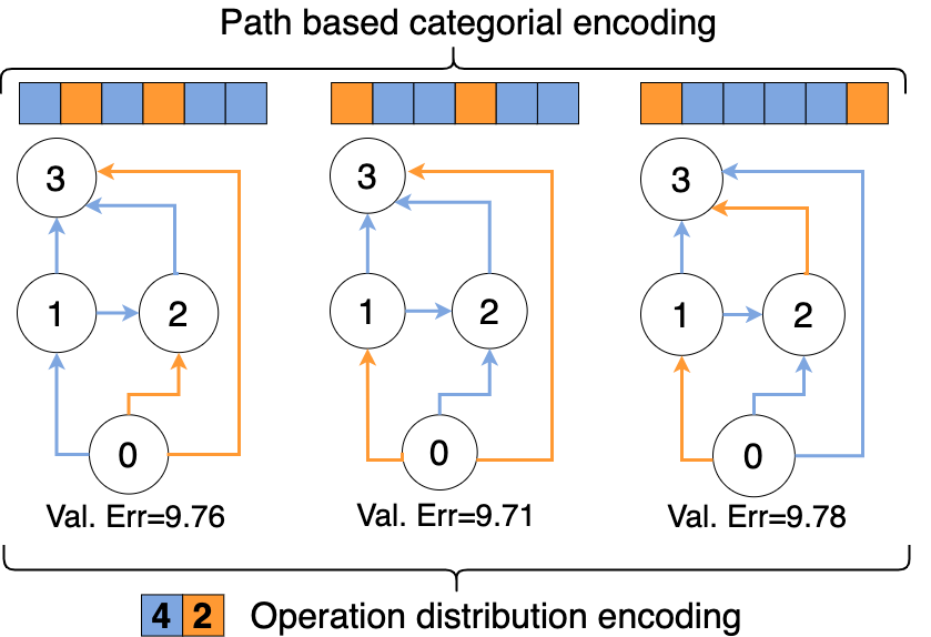
Figure 1: Three architecture cells from nb201 [11] giving very similar validation performance. Each edge represents an operation: either conv1$\times$1 or conv3$\times$3. From the viewpoint of existing encodings, they represent three distinct architectures which all need to be evaluated. The anasod framework assumes that they all belong to the same operation distribution ($4\times$conv3$\times$3 and $2\times$conv1$\times$1 in 6 operations) and does not repeatedly re-evaluate each one.

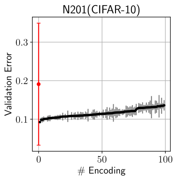
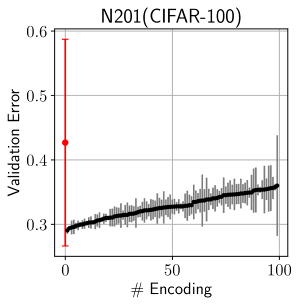
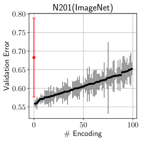
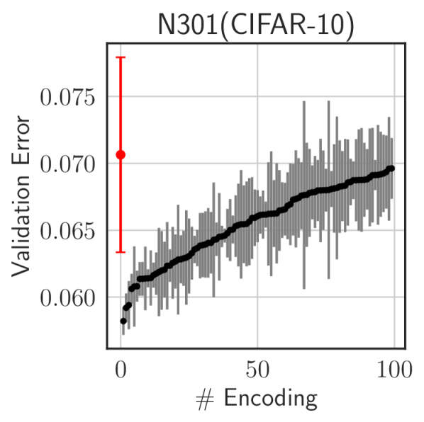
Figure 2: To what extent does the anasod encoding determine performance? We randomly draw $200$ anasod encodings in 4 tasks. Within each, we draw $5$ architectures for each encoding and show the mean $\pm$ 1 standard deviation (black and gray, respectively) of the top-100 encodings vs those of all 1,000 sampled architectures (red). Architectures sampled from the same encoding usually perform similarly and encodings that on average perform better also have smaller variability.

Knowing that most architectures perform similarly and that the true global optimum is very unlikely to be found, one can ask whether the current paradigm of searching for a specific architecture is the way forward. Differently from prior work, we argue that tackling nas with an approximate algorithm that learns a distribution rather than a specific architecture allows resources to be used more efficiently. An intuitive understanding can be had from Figure 1. Indeed, the accuracy distribution for each encoding is shown to have small standard deviation in Figure 2, which motivates the optimization over encodings rather than architectures. The key issue is that comparing every single architecture is intractable and unnecessary: intractable due to the sheer size of the considered search spaces, and unnecessary because we experimentally know that small differences in the architecture have little to no effect on the final result [46, 34, 49].

Rather than searching for a specific architecture, we propose to find an approximate solution by instead searching for the optimal operation distribution, defined as the relative ratio between operations (e.g. conv3$\times$3, conv5$\times$5, maxpool, …) in the whole architecture. Once the operation distribution is defined, we can sample from it, seamlessly generating architectures of variable length. As we experimentally show, this simple re-framing of the nas problem enables us to significantly improve the sample efficiency of all exploitative methods. Indeed, anasod is orthogonal to existing nas solutions and we experimentally show how it improves over Bayesian optimisation, local search and random search. Not only is this approach more sample-efficient, but it has less potential for overfitting, as we show by successfully transferring to new datasets.

To summarise, we propose searching for an approximate rather than exact solution to the nas problem. This is easily applicable to most existing approaches and enables a substantial speed-up (from sample-efficiency) without a sacrifice in performance. We empirically show this both on the nas benchmarks [11, 38] and with open-domain experiments on cifar-10 and cifar-100.

2 Related Work

Architecture encodings Several encoding schemes have been proposed to embed the directed acyclic graph of an cell-based architecture into a real-valued tensor to facilitate optimisation [43]. These encodings either represent the architecture via a flattened adjacency matrix and a list of operations [50] or characterise the architecture as a set of paths from input to output [44]. While multiple architectures may be projected to the same encoding and thus a particular encoding can also define a distribution of architectures, such performance standard deviation is rather small [43] and the search dimension remains high. On the other hand, some prior works use graph neural networks [37], graph kernels [35] or variational autoencoders [29] to implicitly encode an architecture. These methods all require surrogate training and focus on comparing individual architectures rather than distributions of architectures.

Stochastic methods Recently, a number of methods based on probabilistic formulations have been proposed to overcome the memory requirements of differentiable approaches [6, 48, 5]. These works learn a distribution over architectures and, at a first glance, might appear similar to what is being proposed in this work. The differences are significant and two-fold: (1) first and foremost the output of these methods is a deterministic architecture and the distribution is learned for each possible placement of an operation—which does not reduce the search space size; and (2), their focus is strictly applied to the one-shot methods only. In other words, these works [6, 48] propose a different search strategy rather than a different encoding, and as such are orthogonal to anasod and could be combined with it. Another related class of works propose the concept of stochastic architecture generators [46, 34]. Specifically, they employ random graph generators to define the wiring pattern within an architecture and thus recast the problem of searching for an optimal architecture to finding the optimal generator hyper-parameters [34]. This significantly reduces the dimension of the search space and improves the search efficiency. However, these prior works focus on the graph architecture topology, while keeping the operation type fixed. On the other hand, the focus of our work is to show that, regardless of any specific cell types, the operation distribution is an efficient and informative representation.

3 Our Method: ANASOD

3.1 Overview

Searching for the optimal configuration of an architecture cell can be both extremely difficult (due to the formulation of nas as a combinatorial optimisation problem) and ineffective (due to the common practice of using different pipelines during search and evaluation and the imperfect correlation of performance between the two). Instead, we propose to learn the optimal distribution of operations within a cell. Formally, given an architecture cell $C$ with $N$ operation blocks $\{n_{1},...,n_{N}\}$ where each operation is chosen from a pool of $\{o_{1},...,o_{k}\}$ candidate operations (e.g. in the nb201 cell, we have $N=6$ and $k=5$), its normalised distributional encoding (which we term the anasod - Approximate nas via Operation Distribution - encoding) $\tilde{\mathbf{p}}$ is a $k$-dimensional vector defined over the $k$-dimensional probability simplex $\{\tilde{\mathbf{p}}\in\mathbb{R}^{k},\sum_{i=1}^{k}\tilde{p}_{i}=1,\tilde{p}_{i}\geq 0\;\forall i=\{1,\dots,k\}\}$ where $\tilde{p}_{i}=\frac{n(o_{i})}{N}$ and $n(o_{i})$ is the number of blocks in the cell $o_{i}$. The unnormalised encoding is $\mathbf{p}=N\tilde{\mathbf{p}}$.

Because the encoding now only incorporates information about the operations in the cell, a single encoding maps to a distribution of architectures sharing the same distribution of operations but possibly with different wiring. A key feature of anasod is the easy reversibility in decoding $\tilde{\mathbf{p}}$ back to a distribution of architectures defined by it $p(\alpha|\tilde{\mathbf{p}})$: Here we outline two possible ways to achieve so which are asymptotically equivalent when either the size of the cell becomes large, or when are sampling a large number of architectures. First, we may directly interpret the $i$-th element of the unnormalised encoding vector $\mathbf{p}=N\tilde{\mathbf{p}}$ as the number of operation $i$ in the cell $C$; with the operations fixed, we may then randomly shuffle their ordering and the wiring amongst them to obtain a set of architectures $\{\alpha_{1},\alpha_{2},\dots\}$ This, however, requires $\sum_{i=1}^{k}p_{i}=N$ and $\mathbf{p}\in\mathbb{N}^{k}$.

Correspondingly, $\tilde{\mathbf{p}}$ is only defined on a regular grid on the $k$-simplex, which could be problematic if we would like to apply standard continuous optimisation on the encoding space. To overcome this, we utilise the following rounding rule proposed in [4] to “snap” an arbitrary point on the simplex to a valid, all-integer configuration: denoting the standard $k$-simplex on which the unnormalised encoding lies as $\Delta^{k}$ and an arbitrary point as $\mathbf{m}$. Define the fractional part of $\mathbf{m}$ as $\mathbf{s}(\mathbf{m})=\big{[}m_{i}-\left\lfloor{m_{i}}\right\rfloor\big{]}_{i\in[1,k]}$, we have $g(\mathbf{m}):=\sum_{i=1}^{k}s(m_{i})=N-\sum_{i=1}^{k}\left\lfloor{m_{i}}\right\rfloor\in[0,k-1]$ as a non-negative integer. We then round $g(\mathbf{m})$ largest elements of $s(m_{i})$ to $1$ and the rest to $0$ to obtain a rounded integer vector $\mathbf{m}_{r}$:

which, as [4] prove, is the closest valid configuration on $\Delta^{k}$ to $\mathbf{m}$ with respect to all $\ell^{p}$-norms for $p\geq 1$.

The second decoding method uses a probabilistic interpretation, and does not constrain $\tilde{\mathbf{p}}$ to a finite set of points. At each operation block $n_{j}\;\forall j\in[1,N]$, we draw a sample from the categorical distribution parameterised by $\tilde{\mathbf{p}}$:

$$n_{j}\sim\mathrm{Cat}(\tilde{p}_{1},...,\tilde{p}_{k})\;\forall j\in[1,N]$$ (2)

While the cells sampled via this decoding method only have operation distribution to be $\mathbf{\tilde{p}}$ on expectation, in this case $\mathbf{\tilde{p}}$ is not constrained to the grid like before, enabling gradient-based continuous optimisation to be used effectively and as we show in Sec. 3.2, is key for applying anasod in the differentiable nas setting.

Table 1: Overall sd, median sd of different architectures sampled from the same encoding and the median sd of the same architecture trained with different seeds. All sd are w.r.t validation error in percentage.

Benchmark	nb201			nb301
Task	C10	C100	ImageNet16	C10
Overall	$9.5$	$14$	$10$	$0.77$
Median (same encoding)
- All encodings	$1.2$	$2.4$	$2.7$	$0.25$
- Top $50\%$-performing	$0.84$	$1.4$	$1.9$	$0.22$
Median (different seeds)	$0.19$	$0.35$	$0.36$	$0.17$

For the proposed encoding to provide a reasonable approximation of the nas solution, it is imperative for the architectures sampled from the same encoding to perform similarly, which we empirically show to be the case in the popular cell-based search spaces represented by the nb201 [11] and NAS-Bench-301 (nb301) [38] datasets. With reference to Figure 2 and Table 1, in each of the $4$ tasks considered, we draw $200$ random encoding $\tilde{\mathbf{p}}$ and within each encoding, we draw $5$ unique architectures sampled from that encoding and query the validation performance of all $1,000$ architectures. To investigate the extent to which anasod encoding determines the validation performance, we compute the overall sd across all sampled architectures which acts as an unbiased estimate of the performance variability over the entire search space, We also consider the median sd amongst architectures sharing the same encoding, with particular attention to the better-performing encodings in which nas is particularly interested. Additionally, we also report the median sd of the same architectures trained with different seeds, representing the amount of irreducible aleatory uncertainty due to evaluation noise. It is evident that fixing the anasod encoding massively reduces the validation error variability and hence is highly predictive of the performance, and comparatively, better encodings have lower variability.

Having established the validity of anasod, we now argue there are 3 key advantages of anasod. First, it requires no learning and massively compresses the search space, yet remains predictive enough about the performance of the architectures. While as discussed, the original architecture space explodes exponentially as $k^{N}$, the number of unique anasod encoding is simply $\binom{N+k-1}{k-1}$. For instance, in the darts-like cell with $k=8$ and $N=14$, the number of architectures is $8^{14}\approx 4.3\times 10^{12}$, but the number of anasod encodings is only $\binom{21}{7}\approx 1.2\times 10^{5}$. This enables us to reduce the difficult combinatorial nas optimisation into a much more tractable, easier-to-solve problem and thus to achieve superior sample efficiency – this is a result of anasod being an approximate encoding; exact encoding such as the adjacency or path encoding, while representing the architecture in a way that is amenable for predictor learning, usually do not reduce the optimisation difficulty per se. Second, as mentioned, we may generatively sample architectures from the encoding easily. This allows us to directly search for an optimal encoding $\tilde{\mathbf{p}}^{*}$ first and to map back to the architectures thereafter for effective (approximate) global optimisation over the entire search space; this is in contrast with many previous approaches which, although using advanced encoding schemes, still rely on random sampling and/or mutation algorithm in the architecture space for architecture optimisation [35, 37, 44]. Lastly, unlike most existing encodings, anasod is defined on a well-studied simplex space with well-defined distance metrics and is of a modest dimensionality; all of which are key for effective deployment of model-based methods such as Gaussian Process (gp)-based Bayesian optimisers, which are often difficult to apply nas due to the high-dimensional search spaces and/or the lack of natural distance metrics.

3.2 Applying ANASOD

In this section, we give some examples that orthogonally combine various methods with anasod to achieve improved efficiency, performance, or both. It is worth emphasising that the methods proposed here are exemplary, and in no way exhaust the applicability of the proposed encoding.

Random Search (rs)

While simplistic in implementation, rs is shown to be a remarkably strong baseline in nas where even the state-of-the-art optimisers often fail to significantly outperform rs [50, 11, 49]. Implementing random sampling in the proposed encoding space is trivial: to sample uniformly from the entire search space, we simply draw encoding from the uniform Dirichlet distribution $\tilde{\mathbf{p}}_{i}\sim\mathrm{Dir}(1,...,1)$. More importantly, by virtue of the unique property that our encoding lies on a probability simplex on which well-principled distributions can be easily defined, we also propose a simple modification that mitigates the key shortfall of rs, the fact that it is purely exploratory and does not exploit the information gathered as the optimisation progresses: at iteration $t$, instead of randomly drawing the next encoding $\tilde{\mathbf{p}}_{t+1}$ from the uniform distribution, we instead draw randomly the next sample from the following distribution whose mode is $\tilde{\mathbf{p}}^{*}$, the best-performing encoding seen so far:

$$\tilde{\mathbf{p}}_{t+1}\sim\mathrm{Dir}(\alpha_{1},...,\alpha_{k})\text{ where }\alpha_{i}=k\beta_{t}\tilde{p}^{*}_{i}+1\text{ }\forall i,$$ (3)

where $\beta_{t}$ is a parameter similar to the temperature parameter in simulated annealing that monotonously increases from $0$ (the uniform Dirichlet) to some positive $\beta_{T}$ at termination of the search that controls the scale of the Dirichlet distribution. Essentially, in this modified rs (which we term biased rs), we add exploitation by progressively biasing the generating distribution of the encoding to the locality around the best encoding seen so far with the hope of finding even better ones, with $\beta_{t}$ controlling the amount of exploitation-exploration trade-off. This modification is simple, poses almost no additional computing cost (apart from the need to track $\tilde{\mathbf{p}}^{*}$ as the search progresses), and is orthogonal to other modifications of rs (e.g. rs with successive halving [23] and rs with parameter sharing [25]), but as we will show in Sec. 4 it significantly improves on the vanilla rs on a wide range of search spaces to a level that often matches or even exceeds more sophisticated methods, and thus could serve as a strong baseline for the nas community.

Differentiable NAS

Another popular paradigm in nas is that of Differentiable Neural Architecture Search (dnas) pioneered by [28], which, generally speaking, utilises continuous relaxation of the discrete architecture space (followed by discretisation at the end of the pipeline) with weight-sharing supernets so that standard first-order optimisers commonly used in deep learning might be applied in this context. Differentiable nas finds reasonable solutions, and often offers a massive speedup compared to earlier query-based methods, but it is also subjected various criticisms, such as the so-called rank disorder between the found cells during search and evaluation and the unstable training with a propensity to collapse into cells with parameterless operations that corresponds to poorly-performing architectures [49, 54] In this section, we describe a prototypical application of anasod in the context of dnas, and shows that it performs competitively and leads to further saving in computation over the already efficient dnas pipeline while remaining much simpler than many of the existing methods.

To apply anasod in the differentiable setting, we first notice that the stochastic interpretation of the anasod encoding (described in Section 3.1) as the parameters governing the categorical distribution at each operation block $j\in[1,N]$ of a cell. As described, this relaxes the constraint that anasod encoding is only defined on a regular grid (the encoding only needs to obey $\sum_{i}\tilde{p}_{i}=1$). With this, we might compute the derivative of the supernet validation loss $\mathcal{L}_{\mathrm{val}}(\tilde{\mathbf{p}},w)$ w.r.t the encoding, $\nabla_{\tilde{\mathbf{p}}}\Big{(}\mathcal{L}_{\mathrm{val}}(\tilde{\mathbf{p}},w)\Big{)}$ where $w$ is the supernet parameter weights. We formulate the procedure as a bi-level optimisation problem like [28], and include an algorithmic description in Algorithm 1.

Algorithm 1 anasod-dnas. Key differences from existing dnas algorithms marked blue.

1:  Create a mixed operation $\bar{o}^{j}\sim\mathrm{Cat}(\tilde{\mathbf{p}})$ for each operation block. Note that the parameters of the categorical distribution are shared.

2:  while not converged do

3:     Update the encoding $\tilde{\mathbf{p}}$ by descending $\nabla_{\tilde{\mathbf{p}}}\Big{(}\mathcal{L}_{\mathrm{val}}(\tilde{\mathbf{p}},w)\Big{)}$, and keep $w$ constant

4:     Enforce the simplex constraint $\tilde{\mathbf{p}}\leftarrow\frac{\tilde{\mathbf{p}}}{\sum_{i}^{k}\tilde{p_{i}}}$ (i.e. mirror descent)

5:     Update the supernet weights $w$ by descending $\nabla_{w}\mathcal{L}_{\mathrm{train}}(\tilde{\mathbf{p}},w)$, and keep $\tilde{\mathbf{p}}$ constant.

6:  end while

7:  Sample cells from the optimised encoding $\alpha\sim p(\alpha|\tilde{\mathbf{p}}^{*})$ and stack them into a final neural architecture.

While we inherit some key elements from the existing dnas algorithms such as the idea of bi-level optimisation and most hyperparameter choices (e.g. the learning rate of the architecture optimiser and the network architecture), there are two key differences: first, inspired by our fundamental observation that often determining the operation mix is already sufficiently predictive of the architecture performance, we use the $k$-dimensional anasod encoding of the cell as the parameters of the single categorical distribution that governs the all edges in the cell; on the other hand, existing methods uses a $k$-dimensional vector at each edge, leading to a matrix parameterisation of the cell of dimensionality $N\times k$; as we will show later, we argue that our simpler representation implicitly regularises the architecture learning and avoids the catastrophic collapse of many dnas methods due to over-fitting; at the same time, the reduced dimensionality allows fast convergence as we will demonstrate. Second, instead of taking $\arg\max$ of the categorical distribution parameters on each edge at the end of the search, which is hypothesised as a key reason leading to rank disorder (as the discretised architecture might differ a lot from the continuously relaxed architecture in the parameter space [49, 51, 54]), we simply sample architecture cells from the anasod-encoding at the end to build a final network.

Local Search (ls)

At the other end of the exploration-exploitation continuum, ls is purely exploitative, and has recently been shown to be an extremely powerful optimiser, achieving state-of-the-art performance in small search spaces but fails to perform on larger ones [45]. We show that combining anasod with ls universally further improves performance on ls but particularly in the latter case, addressing the previous failure mode of ls. The readers are referred to App. B for a detailed discussion.

Sequential Model-based Optimisation (smbo)

smbo algorithms, in particular Bayessian Optimisation (bo), have seen great success in hyperparameter optimisation due to their exploitation-exploration balancing, sample efficiency, and principled treatment of and robustness against noises that inevitably arise in real life. Nonetheless, their application in nas has been somewhat constrained, partly due to the discrete search space, extreme dimensionality of the existing encoding and the common lack of well-defined distances in such space (the presence of which is crucial for kernel-based methods, such as gp). As discussed, anasod addresses all the three aforementioned issues and enables gp-based bo to be effectively used. anasod-bo is described in Algorithm 2. Nonetheless, we emphasise that anasod-bo is not restricted to the gp surrogate; as we show in Sec. 4, it may also be used with Neural Ensemble Predictor (nep) proposed in [44] to deliver further performance improvements.

For easy parallelism which is key in nas, we opt for a sampling-based optimisation of the acquisition function which allows trivial modifications to be able to recommend batches of points simultaneously, although we are nonetheless compatible with, for example, the common gradient-based optimiser. On this, in addition to the usual bo components, inspired by the recent trust region-based innovations in bo literature [13, 39] we also adopt dynamic adjustment of the encoding generating distribution (Lines 2 and 9 in Algorithm 2). Specifically, similar to anasod-rs, we use the knowledge gained previously (i.e. the location of the best encoding so far $\tilde{\mathbf{p}}^{*}_{t}$ as a prior to generate samples for the next iteration by biasing the Dirichlet distribution. However, instead of using a simple annealing schedule for the $\beta$ parameter, here we adopt a probabilistic trust-region setting, where we halve $\beta$ (i.e. reducing the concentration of the Dirichlet density around $\tilde{\mathbf{p}}^{*}$ to allow candidate encodings to be drawn from a larger region) upon successive successes in reducing the best function value seen so far $y^{*}_{t}$ up to 0. Conversely, we double $\beta$, which is equivalent to increasing the concentration of the Dirichlet p.d.f around the mode and thus to shrink the trust region size upon successive failures, up to a certain $\beta_{\max}$.

Algorithm 2 anasod-bo. Key differences from conventional bo are marked blue.

1:  Input: Objective function (default: validation error) $y$, number of initialising random samples $n_{\mathrm{init}}$

2:  Initialise the encoding generating distribution to the uniform Dirichlet distribution $p(\tilde{\mathbf{p}})=\mathrm{Dir}(1,...,1)$

3:  Sample $n_{\mathrm{init}}$ random encodings $\tilde{\mathbf{p}}_{[1:n_{\mathrm{init}}]}\sim p(\tilde{\mathbf{p}})$ and evaluate to obtain $y(\tilde{\mathbf{p}})$ to initialise the surrogate gp.

4:  for i=$n_{\mathrm{init}}$,,,.T do

5:     Sample a pool of $B$ candidate encodings from $p(\tilde{\mathbf{p}})$

6:     Select the next query point(s) by identifying the encoding that maximises the acquisition function $\tilde{\mathbf{p}}_{i}=\arg\max\big{(}\mathrm{acq}(\tilde{\mathbf{p}})\big{)}$.

7:     Evaluate a single architecture $\alpha_{i}$ from the encoding $\tilde{\mathbf{p}}_{i}$ to approximate the performance of all architectures parameterised by $\tilde{\mathbf{p}}_{i}$.

8:     Augment the surrogate gp with new encoding-observation pair(s) $\mathcal{D}_{i}\leftarrow\mathcal{D}_{i-1}\cup\{\tilde{\mathbf{p}}_{i},y(\tilde{\mathbf{p}}_{i})\}$ and optimise the gp hyperparameters via the marginal log-likelihood maximisation.

9:     Update the encoding generating distribution $p(\tilde{\mathbf{p}})$.

10:  end for

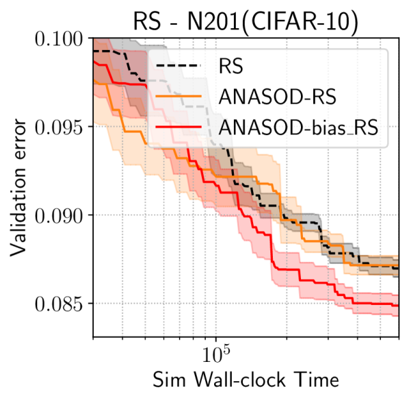
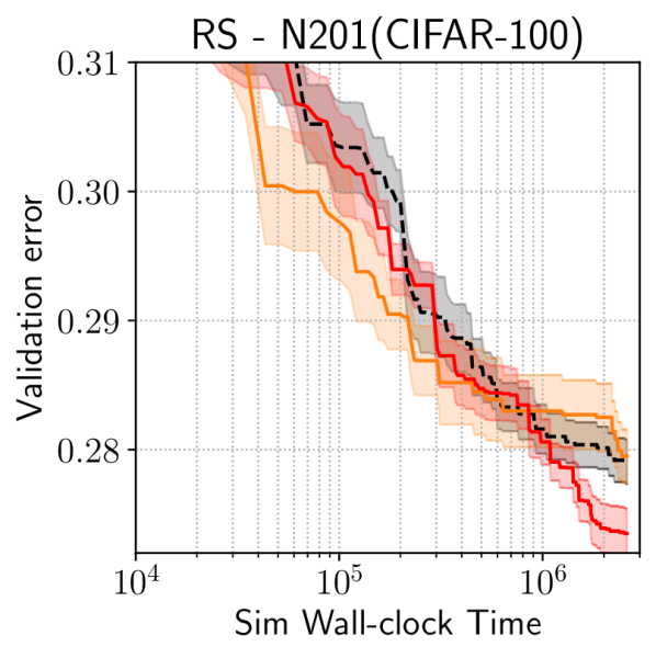
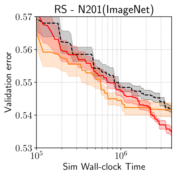
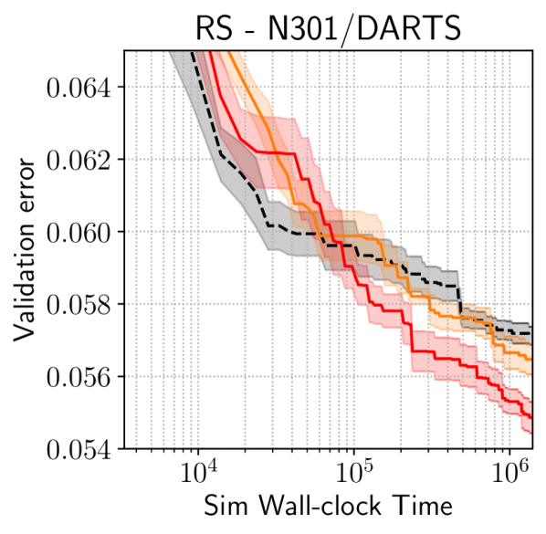
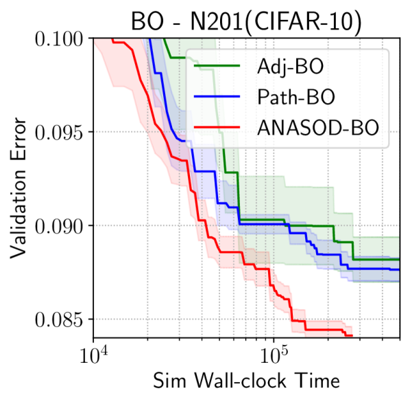
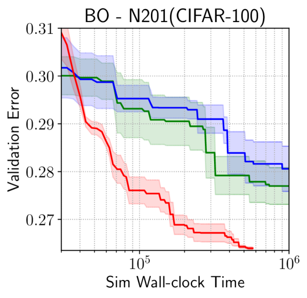
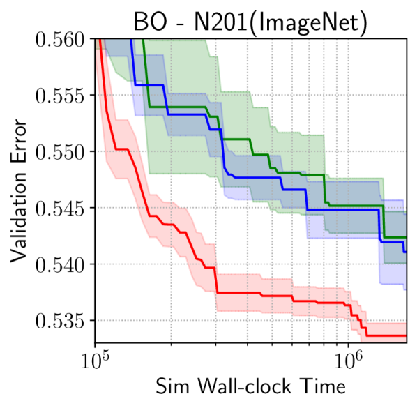
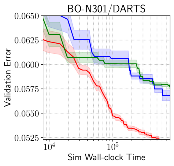
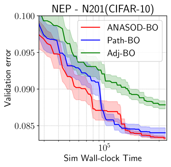
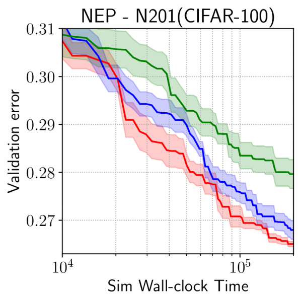
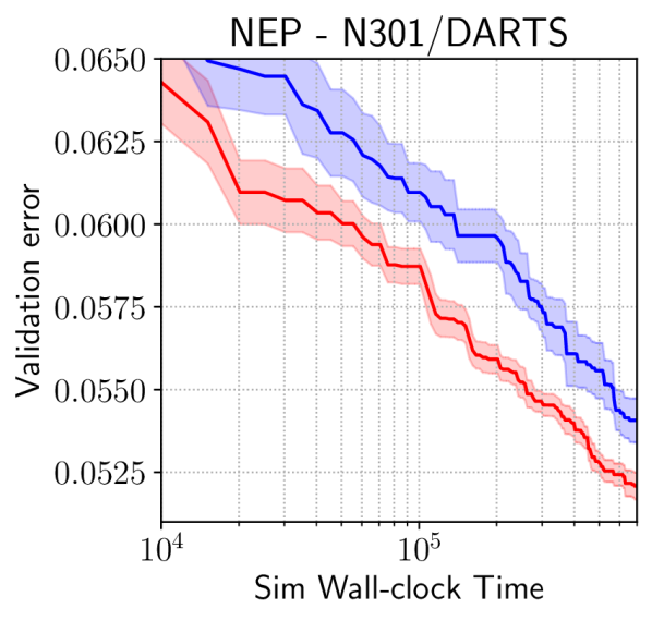
Figure 3: Performance of various methods on nb201 and nb301 with and without the anasod encoding: (Top row) random search, rs; (Middle row) gp-bo; (Bottom row) nep-bo. Note the x-axis which shows the (simulated) gpu-seconds is in log-scale. For rs we set a budget of maximum 300 architecture queries; for bo, we set a more stringent budget of 150 queries for anasod-bo but allow the baselines to run for longer (to observe the amount of speedup). Adj-bo and Path-bo are the variants of bo that are otherwise identical to anasod-bo as outlined in Algorithm 2, but with the anasod encoding replaced by the adjacency [55, 50] and path [44, 42] encoding, respectively. Lines and shades denote mean $\pm$ 1 standard error, across 10 different random trials.

Since we conduct bo on the encoding space directly, at termination anasod-bo returns the optimised encoding $\tilde{\mathbf{p}}^{*}$ instead of a single architecture $\alpha^{*}$. This may be of independent benefits: for example, the anasod encoding, which has much fewer parameters than an exact architecture cell and its exact encoding thereof, should be much less prone to overfitting to a singular data-set which is cited as a problem many nas methods have [26]. Furthermore, since multiple architectures are sampled from a single encoding, we might also obtain an ensemble of architectures which is recently shown to perform very competitively both in terms of accuracy and uncertainty quantification [2, 53]. We defer a thorough investigation to a future work.

4 Experiments

Table 2: Performance on NAS-Bench datasets. Unless otherwise specified, we report mean $\pm$ 1 standard error of the validation error across 10 random trials. For fair comparison, in rs and ls experiments, the numbers shown denote the best validation error seen after $\mathbf{300}$ architecture queries; in bo experiments, we show the best validation error seen for each method after $\mathbf{150}$ architecture queries (which is the budget we set for anasod-bo).

Benchmark	nb201			nb301
Dataset	cifar-10	cifar-100	ImageNet16	cifar-10
rs	$8.67_{\pm 0.03}$	$27.91_{\pm 0.17}$	$54.17_{\pm 0.10}$	$5.71_{\pm 0.02}$
anasod-rs	$8.71_{\pm 0.05}$	$27.95_{\pm 0.20}$	$53.85_{\pm 0.12}$	$5.65_{\pm 0.04}$
anasod-biasedrs	$\mathbf{8.48}_{\pm 0.06}$	$\mathbf{27.35}_{\pm 0.20}$	$\mathbf{53.30}_{\pm 0.10}$	$\mathbf{5.47}_{\pm 0.04}$
RL [55]	$8.91_{\pm 0.05}$	$28.15_{\pm 0.18}$	$54.45_{\pm 0.12}$	*
RE [33]	$8.86_{\pm 0.05}$	$28.40_{\pm 0.14}$	$54.28_{\pm 0.10}$	$5.62_{\pm 0.03}$
SMAC [18]	$8.89_{\pm 0.05}$	$27.80_{\pm 0.20}$	$53.64_{\pm 0.13}$	$5.45_{\pm 0.03}$
TPE [3]	$8.57_{\pm 0.04}$	$27.28_{\pm 0.14}$	$53.54_{\pm 0.14}$	$5.51_{\pm 0.02}$
GCNBO [37]	$8.84_{\pm 0.01}$	$27.93_{\pm 0.03}$	$53.46_{\pm 0.06}$	$5.54_{\pm 0.04}$
BANANAS [44]	$8.51_{\pm 0.08}$	$26.53_{\pm 0.02}$	$53.41_{\pm 0.04}$	$5.36_{\pm 0.05}$
NAS-BOWL [35]	$8.50_{\pm 0.09}$	$26.51_{\pm 0.00}$	$\mathbf{53.36}_{\pm 0.04}$	$5.31_{\pm 0.06}$
anasod-bo	$\mathbf{8.41}_{\pm 0.05}$	$\mathbf{26.41}_{\pm 0.02}$	$\mathbf{53.36}_{\pm 0.10}$	$\mathbf{5.24}_{\pm 0.02}$
∗: The original repo does not support the nb301 search space.

4.1 Experiments on the NAS-Bench Datasets

We first conduct optimisation experiments on the nb201 and nb301 datasets [11, 38]. On nb201, we consider all three tasks: cifar-10, cifar-100 and ImageNet16. nb301 is a surrogate-based benchmark that is trained on cifar-10 only, but it contains as many distinct architectures as the darts search space and is thus much more challenging. We do not conduct experiment on the earlier NAS-Bench-101 (nb101) [11], as similarly to nb301 it is also only trained on cifar-10, but its search space ($\sim 4\times 10^{5}$ architectures) is much smaller.

Comparison with baseline strategies

To enable direct and fair comparison of algorithms within each class, we first compare rs, gp-bo and nep-bo against their anasod counterpart, as described in Section 3.2.

In the top row of Figure 3, we observe that anasod-rs performs on par with rs—this is unsurprising, as both methods sample uniformly from the same, entire search space which is independent of the specific encoding chosen to represent it. This result also acts as a sanity check that there is no noticeable bias in sampling in the anasod space as contrasted to the original architecture space. On the other hand, anasod-rs with bias, which randomly samples from a non-uniform Dirichlet distribution, can be seen to significantly outperform them both as the optimisation progresses, across all tasks, further highlighting its potential as a simple yet robust baseline in nas research.

The middle row of Figure 3, containing the Gaussian Process based bo experiments, shows that anasod achieves a massive speed-up compared to both the adjacency and path encodings, the two dominant types of encoding in nas [43]. Perhaps owing to the high-dimensional, one-hot-encoded nature of the two alternative encoding, gp-bo struggles to learn meaningful relations and performs no more competitively than rs or ls, at least up to the query budget we consider (e.g. for a simple, $N$-node DAG, the adjacency encoding has $\frac{N(N-1)}{2}+N$ dimensions whereas the path encoding, without truncation, has $\sum_{j=1}^{N}k^{j}$ dimensions [43]. In contrast, anasod encoding only has $k$ dimensions corresponding to the $k$ operation choices). On the other hand, by rigorously compressing the search space, for which non-parametric models such as gp s are better suited, anasod enables the full power of gp-bo to be utilised.

We show the results on nep-bo in the bottom row of Figure 3. The findings are consistent with those on gp-bo discussed above although Path-bo performs much stronger. This is unsurprising, as nep-bo is originally proposed to be used with the path encoding [44], and that the hyperparameters we used are tuned for this purpose. Nonetheless, on nb201 search spaces, anasod encoding delivers significant speedup, whereas on the more difficult nb301 search space, it is also significantly better in terms of final performance.

Comparison with SOTA

We also compare our anasod-based gp-bo with a wide range of competitive baselines, including reinforcement learning (rl [55]), regularised evolution (re [33]), Sequential Model-based Algorithm Configuration (smac [18]), Tree-structured Parzen Estimator (tpe [3]), graph convolutional network based bo (gcnbo [37]), nep-bo with path encodings (bananas [44]) and Weisfeiler–Lehman kernel-based bo (nas-bowl [35]). Similarly, we compare anasod-dnas with a number of existing dnas algorithms in Table 3. All additional details about the experimental setup can be found in App. A.

Table 3: Comparison of one-shot nas methods on nb201. To reflect real-world applications, we search on cifar-10 and transfer the search result to the other datasets.

Benchmark	Search	nb201
Dataset	epoch	cifar-10	cifar-100	ImageNet16
Optimal	-	$5.70$	$26.50$	$52.70$
RSPS∗ [25]	$50$	$12.34_{\pm 1.7}$	$41.67_{\pm 4.3}$	$68.86_{\pm 3.9}$
DARTS† [28]	$50$	$45.70_{\pm 0.0}$	$84.39_{\pm 0.0}$	$83.68_{\pm 0.0}$
SETN∗ [10]	$50$	$12.36_{\pm 0.0}$	$41.95_{\pm 0.2}$	$67.48_{\pm 0.2}$
ENAS† [32]	$50$	$45.70_{\pm 0.0}$	$84.97_{\pm 0.0}$	$83.68_{\pm 0.0}$
GAEA-DARTS∗ [24]	$25$	$8.36_{\pm 2.6}$	$31.61_{\pm 4.5}$	$58.41_{\pm 4.2}$
anasod-dnas	$20$	$7.75_{\pm 1.2}$	$31.33_{\pm 1.7}$	$58.00_{\pm 2.9}$
∗: Results taken from [24]; †: Results taken from [11].

From Table 2, it is evident that anasod-bo clearly outperforms competing methods, with the only bananas and nas-bowl being relatively close competitors in terms of final validation error. For nas-bowl, we hypothesise that this could be because it relies on local mutation in the architecture space for candidate architecture generation (at each bo iteration, the algorithm generates a pool of candidates from which bo recommends the next evaluation), which might be overly greedy and exploitative and miss the better solution especially on larger and hence more complicated search spaces. For bananas, the performance gain mainly comes from the nep (which is orthogonal to anasod), as we show previously, combining anasod with nep also yields further improvements. With respect to Table 3, despite of the much simpler formulation, anasod-dnas performs competitively, outperforming all baseline methods significantly with the exception of gaea-darts where they perform on par (note that we consider gaea-darts with bi-level formulation since our implementation of anasod-dnas is also bi-level. While the single level version of gaea-darts outperforms the bi-level counterpart, this modification is orthogonal to our contribution, and hence could potentially be similarly exploited by anasod-dnas for further performance gains). Furthermore, as we show the learning curves in Fig 5 in App. C, anasod-dnas almost instantly converges to a location of good solutions, allowing us to shorten the search time – this is possible because anasod encoding compresses and smooths the search space into a comparatively low-dimensional vector, allowing more effective gradient-based optimisation. Furthermore, in contrast to the previously mentioned performance collapse observed in some dnas methods [11], the performance of anasod-dnas does not drop as optimisation proceeds.

4.2 Open Domain Experiments

For these experiments, we choose the popular nasnet-style search space [56], In our experiments, we use the setup of lanas [41, 40] and due to the much higher computational cost, we only experiment with anasod gp-bo. It is worth noting that due to the distributional nature of the anasod encoding, differing from all previous nas methods, we do not search for a single cell, but we instead search for an encoding: at training and evaluation time, we randomly draw concrete realisations of architecture at each layer by sampling the encoding according to the decoding scheme described in Section 3.1. To highlight the sample efficiency of our method, during search we only sample and train $50$ architectures for $30$ epochs each. At the end of the search phase, we re-train the architecture corresponding to the best encoding seen to evaluate its performance.

Table 4: Performance on cifar-10 in the nasnet-style search space. anasod-bo experiment is conducted on $4\times$ NVIDIA Tesla V100 gpus using $0.6$ wall-clock days.

Algorithm	Val. Err	#Params(M)	Method
Random-WS [46]	$2.85_{\pm 0.08}$	$4.3$	RS
NASNet-A [56]	$2.65$	$3.3$	RL
LaNAS [41]	$2.53_{\pm 0.05}$	$3.2$	MCTS
DARTS [28]	$2.76_{\pm 0.09}$	$3.3$	GD
DARTS+† [27]	$2.37_{\pm 0.13}$	$4.3$	GD
P-DARTS [8]	$2.50$	$3.4$	GD
DropNAS [15]	$2.58_{\pm 0.14}$	$4.1$	GD
DropNAS† [15]	$1.88$	$4.1$	GD
BANANAS [44]	$2.64$	-	BO
BOGCN [37]	$2.61$	$3.5$	BO
NAS-BOWL [35]	$2.61_{\pm 0.08}$	$3.7$	BO
anasod-bo (Mixup)	$2.63$	$3.5$	BO
anasod-bo (CutMix)	$2.41$	$3.5$	BO
anasod-bo +	$1.86$	$3.5$	BO
†: Training protocol comparable to anasod-bo +
MCTS: Monte Carlo tree search; GD: Gradient descent.

We report our results searched and evaluated on the cifar-10 dataset in Table 4, where we include two variants of anasod-bo, which only differ in the final evaluation: anasod-bo + uses a range of additional enhancement techniques including CutMix [52], Auxiliary Towers, DropPath [22], AutoAugment [9] and trains for an extended $1,500$ epochs; anasod-bo does not use AutoAugment and trains for the standard $600$ epochs and we report anasod-bo using two regularisation schemes. Owing to both the shorter search budget and the smaller number of epochs per search (c.f. bananas [44], which trains $100$ architectures for $50$ epochs ($\sim 12$ gpu days), and lanas [41] which trains $800$ architectures ($\geq 150$ gpu days)), anasod-bo is much more efficient than most other query-based nas methods.

Transferring to cifar-100

We then transfer the best encoding searched on cifar-10 to the cifar-100 data-set, and we present the results against a number of competitive baselines in Table 5 (note that some methods use advanced evaluation techniques similar to those used in anasod-bo +, and they are marked correspondingly). Remarkably, the performance obtained by us ($16.33\%$ and $13.76\%$ for anasod-bo and anasod-bo +, respectively), outperforms some methods that are trained and searched on cifar-100 directly, empirically demonstrating the robustness of the anasod encoding across various datasets.

Table 5: Performance on cifar-100 in the nasnet-style search space. The anasod-bo result is transferred from cifar-10.

Algorithm	Val. Err	#Params(M)	Method
DARTS [28]	$17.76$	$3.3$	GD
DARTS+† [27]	$14.87$	$3.9$	GD
P-DARTS∗ [8]	$16.55$	$3.4$	GD
DropNAS [15]	$16.39$	$4.4$	GD
DropNAS+† [15]	$14.10$	$4.4$	GD
anasod-bo∗ (CutMix)	$16.33$	$3.5$	BO
anasod-bo+∗	$13.76$	$3.5$	BO
*: Transferred from the cifar-10 search.
†: Training protocol comparable to anasod-bo +.

5 Conclusion

In this work, we have shown how anasod, an approximate solution to the nas problem by effective compression of the search space, enables a speed-up in search with little to no deterioration in performance. Through combining with various search strategies, we show the versatility and effectiveness of our method on nas benchmarks. We also perform open domain experiments cifar-10, showing competitive performances compared to the state-of-the-art and successfully transfer the encoding (and thus the architecture) to cifar-100. We believe the room for future works is ample: on one side, the operation distribution is a human-interpretable representation to communicate the gist of the architecture. On the other hand, by not restricting the algorithm to a single architecture, anasod can naturally generate diverse ensembles of related and high performing architectures. Ensembles have shown to provide benefits such as robustness [19] and future work should investigate this direction. Furthermore, we have currently only validated the effectiveness on computer vision tasks in popular cell-based nas search spaces, and it would be similarly interesting to verify both alternative search spaces [16] and/or tasks [21, 30]. Finally, as opposed to most existing search strategies, anasod is orthogonal to a large number of different strategies and thus could be effectively combined with ever-improving new strategies for even further improvements.

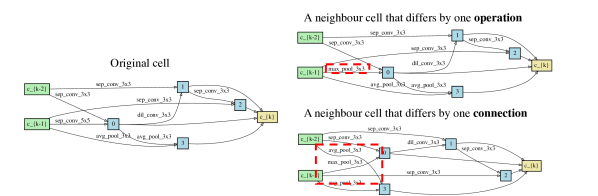
Figure 4: Examples of neighbouring cells in the architecture space. The first neighbour differs by one operation (circled in red) and the second neighbour differs by one connection (note the average pooling block is connected to input c_{k-2} instead of node 0 in the original cell.

Appendices

Appendix A Experimental Setup

In this section we outline the detailed implementation setup for both our method and the baselines we implemented, on both the benchmark and open-domain tasks considered in this paper.

A.1 Benchmark Tasks

Data

We experiment on nb201 and nb301. nb201 has a search space in the form of acyclic directed graph with 4 nodes and 6 edges, with each edge corresponding to a possible operation from conv1$\times$1, conv$\times$3, skip-connect, maxpool and zeroize (zeroize suggests the ending node will regard any input information as zero). The data-set contains 15,625 neural architectures, evaluated exhaustively on 3 image datasets, namely cifar-10, cifar-100 and ImageNet16 (the downsampled ImageNet to $16\times 16$). In addition to standard metrics such as validation and test accuracy/losses, we may also access additional information such as the complete training curve, time spent in training and FLOPs. The dataset and API can be downloaded from https://github.com/D-X-Y/NAS-Bench-201.

nb301 [38] differs from the previous tabular benchmark in that it contains a much larger search space (the search space is identical to the DARTS search space, which contains more than $10^{18}$ unique architectures). Each architecture contains 2 cells, with each cell again being a acyclic directed graph similar to nb201, but with 8 nodes and 14 possible edges. Each edge corresponds to one of a wider range of possible operations, namely separable convolution 3$\times$3, 5$\times$5; dilated convolution 3$\times$3, 5$\times$5; max pooling 3$\times$3, average pooling 3$\times$3, skip connection. Due to the prohibitively large search space it is not possible to exhaustively train each unique neural architecture contained in it. Instead, a large number of query-based nas methods, ranging from the simplest random search to more complicated methods such as bananas [44], are run on this search space to give a good overall coverage by training a large number of architectures. With this large corpus of trained architectures and their corresponding accuracy, an ensemble of surrogate models, including an ensemble of models including LGBoost[20], XGBoost [7] and graph isomorphic networks (GIN) [47], are fit so that given an unknown architecture $G$, we might use the predicted accuracy from this surrogate model as a much cheaper proxy to the true, expensive accuracy that might only be obtained from training the architecture from scratch. Similar to nb201, nb301 similarly provides the additional diagnostic information as listed above. The dataset and the API may be downloaded from https://github.com/automl/nasbench301.

Algorithm Setup

Unless otherwise stated, each method is repeated with 10 random starts and the mean/standard error are reported and where applicable, each method is also initialised with 10 random samples/evaluations at the beginning of the routines.

• Random Search (rs) Both the original rs and the unbiased anasod-rs are hyperparameter free, but due to the presence of bias away from the uniform distribution in anasod-biasedrs, there exists some additional hyperparameters. In our experiments, we set the maximum Dirichlet scale $\beta_{\max}$ (explained in Section 3.2) to be $2$ (i.e. the $\beta$ at the last random search iteration $t=T$), and we use a linear annealing schedule such that the $\beta$ at iteration $t$ is simply $t\frac{\beta_{\max}}{T}$.

• Local Search (ls) For ls, we mainly adapt the implementation available in the repository associated with [43] (available at https://github.com/realityengines/local_search and https://github.com/naszilla/nas-encodings). For the baseline ls, at each iteration the best performing architecture up to the current iteration $t$ ($\alpha^{*}_{t}$) is identified; From this, the algorithm exhaustively enumerates and queries its neighbours, defined in this context as the other architectures $\alpha$ such that each of them only differs from $\alpha^{*}_{t}$ by edit distance of 1 (i.e. only different by 1 operation block or wiring. See Figure 4 for examples of neighbour architectures). The algorithm terminates (and restarts again if there is still unused budget) when it cannot find neighbour(s) to improve the best performance, suggesting that a (local) optimum has been reached.

  In anasod-ls, we use the same procedure but conduct the search in the anasod encoding space instead of the architecture space at the beginning. Specifically, instead of identifying the best performing architecture, we identify the best performing encoding $\tilde{\mathbf{p}}^{*}_{t}$ up to the current iteration $t$ and search its neighbours as described above. In this case, since each valid anasod encoding is a vertex on the regular grid in the $k$-simplex, the neighbours are simply the adjacent vertices on the grid (for example, for a cell with $N=5$ and $k=3$, the neighbours of encoding $[1,1,3]$ are $[0,1,4],[1,0,4],[0,2,3],[2,0,3],[1,2,2]$ and $[2,1,2]$).

• anasod-bo We use a standard Gaussian Process (gp) as the surrogate for anasod-bo with Mátern 5/2 kernel. To improve the goodness of fit of gp, we always normalise the input (in our case, the anasod encodings) into standard hyperrectangular boxes $[0,1]^{k}$. For the targets (in our case, the validation error), we find that using a log-transform often leads to better estimation of the predictive uncertainty, similar to the finding in [35]. We then use a normalisation wrapping around the log-predictive uncertainty by de-meaning the data and dividing by the data standard deviation such that the gp targets are approximately within the range of $\mathcal{N}(0,1)$.

  For the gp hyperparameters, we constrain the lengthscales to be within $[0.01,0.5]$, the outputscale to be in $[0.5,5]$ and the noise variance to be within $[10^{-6}.10^{-1}]$ and by default we do not enable the automatic relevance determination (ARD). The exact hyperparameters of the gp are obtained by optimising the gp log-marginal likelihood and the gp model is implemented using the gpytorch [14] package which feature automatic differentiation.

  For the implementation of the bo routine, we use the expected improvement criterion as the acquisition function that needs to be optimised at each iteration. To optimise the acquisition function to obtain the recommendation from the bo $\arg\max a(\tilde{\mathbf{p}})$, in this paper we use the sample-based optimisation by first randomly generating $100k$ samples via randomly sampling the candidate generating distribution (described in Algorithm 2 in the main text). However, we also explore a gradient-based optimisation approach in to the acquisition function, whose update may be written as:

  $$\tilde{\mathbf{p}}^{\prime}\leftarrow\tilde{\mathbf{p}}-\eta\frac{\partial a(\tilde{\mathbf{p}})}{\partial\tilde{\mathbf{p}}}$$

  $$\tilde{\mathbf{p}}\leftarrow\frac{\tilde{\mathbf{p}}^{\prime}}{\sum_{i}^{k}\tilde{p_{i}}}$$ (4)

  where we conduct mirror descent by combining the gradient-based update (we use the simple gradient descent for simplicity but the optimisation is compatible with gradient-based optimisers such as Adam; here $\eta$ is the generic learning rate for gradient-based methods) with the normalisation to enforce the simplex constraint. We find that both acquisition optimisation methods to be broadly comparable, but it is trivial in concept and implementation to extend the sample-based optimisation technique into batch setting where at each bo iteration, multiple recommendations are produced.

• Other baselines For reinforcement learning (rl), regularised evolution (re), Sequential Model-based Algorithm Configuration (smac), Tree-structured Parzen Estimator (tpe), we use the code available at https://github.com/automl/nas_benchmarks/ for the nb201 search space and adapt the codes for the nb301 repository. For bananas [44], we use the official implementation available at https://github.com/naszilla/bananas; for gcn-based bo, we use the implementation available at NASLib [36] https://github.com/automl/NASLib; for nas-bowl [35], we use the official implementation at https://github.com/xingchenwan/nasbowl. Unless otherwise specified, we use the default settings and hyperparameters in these methods. Since nb301 is to be used as a cheaper proxy to the darts search space, for the baseline methods, we use the default settings for darts search as the settings for the nb301 experiments.

A.2 Open-domain Tasks

For the open-domain tasks we use the popular nasnet-style [56] search space. Since nb301 benchmark already includes the typical darts search space (i.e. nasnet-style search space with 8 nodes and 14 possible edges), here we follow previous works [40, 41] by opting for an enlarged search space with 10 nodes and 20 possible edges, containing order-of-magnitudes more unique architectures even than the standard darts space – this makes the search of a good performing cell within a small number of queries even more challenging. For the implementation details, we largely follow [40, 41, 28] but with two major exceptions: first, as a demonstration of our sample efficiency, we both train much fewer architectures during search time, and train fewer epochs per architecture compared to previous works such as [35, 44, 37]: during search time we use the anasod-bo procedure described above. Second, while [41] restricts the candidate operations to $4$ perceived to be high-performing (max pool, separable convolution 3$\times$3, skip connection and dilated convolution 3$\times$3), we retain the full range of $8$ operation candidates for fair comparison with other previous works. For an encoding $\tilde{\mathbf{p}}$, we sample 24 valid cells randomly to build the architecture (this is possible due to the fact that we may sample architectures from the anasod encoding; previous work typically repeats the identical cell multiple times to build a network), and we train each sampled architecture for 30 epochs using SGD with momentum optimiser with cosine annealed learning rate schedule (learning rate at start $\eta_{0}=0.025$ which anneals to 0 at the 30th epoch; momentum $=0.9$; weight decay = $3\times 10^{-4}$) with a batch size of 96, depth of 24 and initial channel number of 36. We terminate the search after training 50 architectures as described, and select the encoding that leads to the best validation error for evaluation. To utilise the parallel computing facilities, we run anasod-bo with batch size of 4 (at each bo iteration, 4 encodings are generated and recommended for training); it is worth noting that further parallelisation is possible to reduce the wall clock time. For example, it is possible to trivially reduce the wall-clock time to 0.3 days if 8 gpus are used.

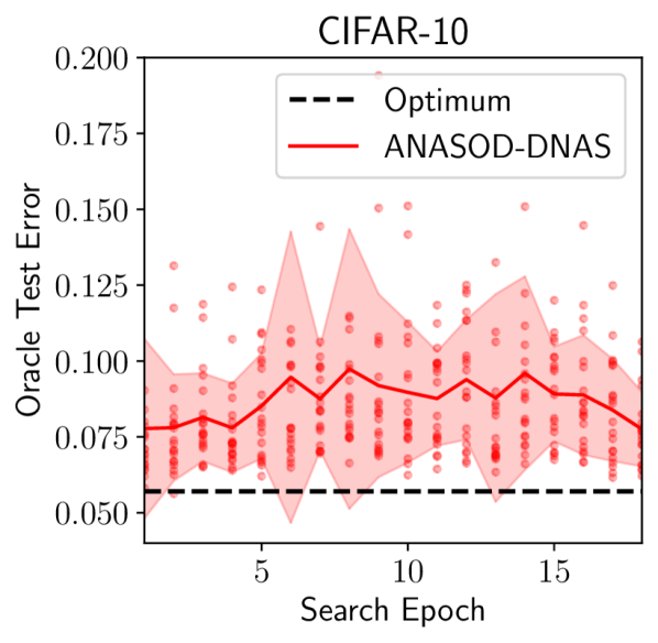
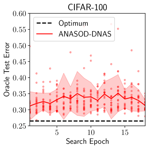
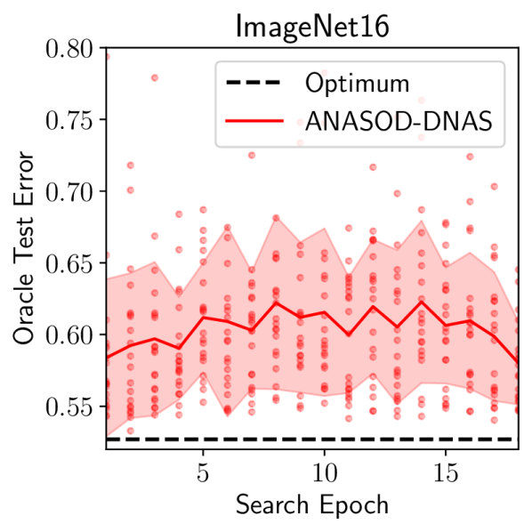
Figure 5: Learning curves of anasod-dnas on nb201 datasets (oracle test error vs the number of learning epochs). We search on the cifar-10 training set and transfer the searched cell directly to the other two datasets. Lines and shades denote mean $\pm$ 1 standard deviation, and dots denote the data points every each trial. Note that unlike previous methods such as darts that quickly collapse to all-skip-connection cells that perform poorly, anasod-dnas converges quickly to good solutions and maintains high performance throughout the optimisation process.

We use two slightly different evaluation procedures and thus report two results, namely anasod-bo and anasod-bo + in Tables 4 and 5 where we largely follow [41]. For the standard, anasod-bo result, we train the architecture induced by the encoding for 600 epochs, again with the SGD with momentum optimiser with initial learning rate set at $\eta_{0}=0.025$ (but the learning rate schedule is now annealed across the entire 600 epochs instead of the 30 epochs described above) and every other hyperparameter is kept consistent with the description above for search. During evaluation, we also include additional augmentation techniques such as CutMix [52], Auxiliary Tower with probability 0.4 and drop path with probability 0.2. For anasod-bo +, we follow previous works such as [27] to increase the training to 1,500 epochs with identical optimiser setting (with the learning rate annealed over 1,500 epochs), and we additionally use AutoAugment. We use the default train/validation partition sets of cifar-10 for both search and evaluation, and for the cifar-100 transfer learning experiment, we directly use the cell searched from cifar-10 for evaluation. The evaluation protocol on cifar-100 is otherwise identical to that on cifar-10 described above.

Appendix B Results on Local Search

Local search has recently been shown to be an extremely powerful optimiser, achieving state-of-the-art performance especially in small search spaces [45]. However, a well-known theoretical and empirical drawback of ls is its susceptibility of getting trapped locally [17, 1], especially when the search space is large and/or is rife with local optima (in the nas context, ls is found to perform much worse in larger search spaces (e.g. darts space) both in [45] and by us in Sec 4.1). To leverage the anasod encoding, we propose a simple modification (which we term anasod-ls in Algorithm 3) which performs ls on the anasod encoding space first and switches to the architecture space when the algorithm fails to improve (i.e. it reaches a local optimum). As discussed, anasod encoding effectively abstracts the huge, original architecture space by compressing multiple unique architectures into a single encoding with fewer neighbours (a neighbour in encoding space is an adjacent vertex on the regular grid on the $k$-simplex), both of which allow ls on the encoding space to make rapid progress on a smoothed objective function landscape. It is worth noting that for this acceleration to be possible, we have to both 1) be able to easily sample architectures from the encoding and 2) have an encoding scheme that compresses and smooths the original architecture search space so that ls is less likely to be stuck. To our knowledge, anasod is the only one that meets both desiderata.

We conduct experiments of anasod-ls on nb201 and nb301 search spaces, and the results are shown in Table 6 and Fig 6. In line with the observation of [45], we observe that the baseline ls performs extremely competitively in the nb201 tasks but struggles in the larger nb301 search space and under-performs even random search—presumably due to the more prevalent local optima that prevents ls from progressing further. However, anasod-ls restores the competitiveness in nb301, and even for the nb201 tasks where the original ls already performs strongly, the use of anasod nonetheless improves its convergence speed in the initial stage of the optimisation. Generally, our experiments show that the margin of improvement increases as the task difficulty increases. Indeed, in the ImageNet task anasod improves both convergence speed and final performance; and in the CIFAR tasks anasod does not improve the final performance further as the baseline is already very close to the ground-truth optimum.

Table 6: Comparison of original ls with anasod-ls. We report mean $\pm$ 1 standard error of the validation error across 10 random trials. Numbers shown denote the best validation error seen after $\mathbf{300}$ architecture queries.

Benchmark	nb201			nb301
Dataset	cifar-10	cifar-100	ImageNet16	cifar-10
LS [45]	$\mathbf{8.34}_{\pm 0.03}$	$26.41_{\pm 0.04}$	$53.43_{\pm 0.08}$	$5.79_{\pm 0.06}$
anasod-LS	$8.36_{\pm 0.02}$	$\mathbf{26.38}_{\pm 0.07}$	$\mathbf{53.07}_{\pm 0.09}$	$\mathbf{5.43}_{\pm 0.04}$

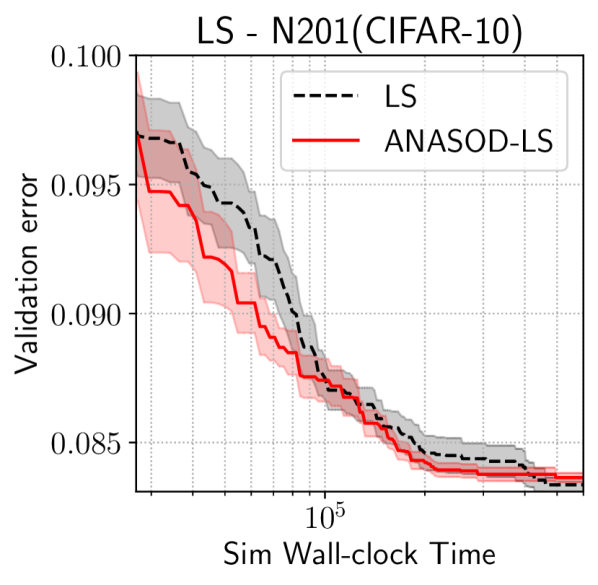
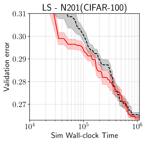
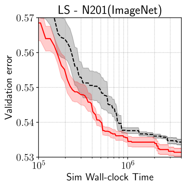
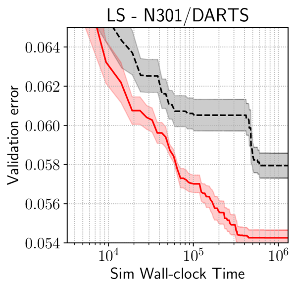
Figure 6: Performance of ls vs anasod-ls on nb201 and nb301. Lines and shades denote mean $\pm$ 1 standard error, across 10 different random trials.

Algorithm 3 Local search. Steps added or modified by anasod-ls are marked blue.

1:  Input: Search space $A$, objective function (default: validation error) $y$

2:  Sample an anasod encoding at uniform $\tilde{\mathbf{p}_{1}}\sim\mathrm{Dir}(1,...,1)$

3:  Evaluate a single architecture $\alpha_{1}$ from the encoding $\tilde{\mathbf{p}_{1}}$ to approximate the performance of the all architectures parameterised by $\tilde{\mathbf{p}_{1}}$: $y(\tilde{\mathbf{p}_{1}})=\mathbb{E}_{\alpha\sim p(\alpha|\tilde{\mathbf{p}})}\Big{[}y({\alpha})\Big{]}\approx y(\alpha_{1}),\alpha_{1}\sim p(\alpha|\tilde{\mathbf{p}})$; denote dummy variable $y(\tilde{\mathbf{p}}_{0})=\infty$.

4:  while $y(\tilde{\mathbf{p}}_{i})\leq y(\tilde{\mathbf{p}}_{i-1})$ do

5:     Search and evaluate the neighbourhood on the encoding space $\tilde{\mathbf{p}}_{i+1}\leftarrow\mathrm{SearchNeighbour}(\tilde{\mathbf{p}}_{i})$.

6:  end while

7:  /* Switch to arch space when ls on encoding reaches an optimum */

8:  if Using anasod-ls then

9:     Sample an arch from the best encoding found : $\alpha_{i}\sim p(\alpha|\tilde{\mathbf{p}}^{*})$

10:  else

11:     Sample an arch uniformly from the search space $A$.

12:  end if

13:  while $y(\tilde{{\alpha}}_{i})\leq y(\tilde{{\alpha}}_{i-1})$ do

14:     Search and evaluate the neighbourhood on the architecture space $\tilde{\alpha}_{i+1}\leftarrow\mathrm{SearchNeighbour}(\tilde{\alpha}_{i})$.

15:  end while

Appendix C Further results on ANASOD-DNAS

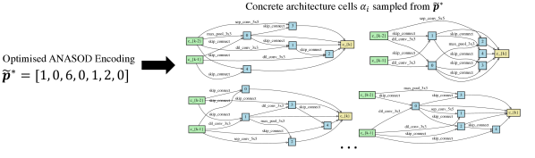
Figure 7: Best encoding found by anasod-bo in the open-domain task (i.e. 1 max pooling, 6 skip connections, 1 separable convolution $5\times 5$ and 2 dilated convolution $3\times 3$) and examples of concrete cells sampled from the optimised anasod encoding. Note that, similar to [44, 41, 35] who use the same cell, we sample the normal and reduction cells from the same encoding.

We show the learning curves of anasod-dnas in Figure 5, where at each training epoch we sample and query the oracle test accuracy of an architecture from the encoding learnt at that point: anasod-dnas almost instantly finds and converges to a location of good solutions, allowing us to shorten the search time while still recovering good solutions – this is possible because anasod encoding massively compresses and smooths the search space into a comparatively low-dimensional vector, allowing gradient-based optimisers to converge efficiently. Furthermore, unlike methods like darts that are shown to lack sufficient regularisation and quickly overfits to find cells dominated by skip-connections that hence perform poorly [11], the performance of anasod-dnas does not drop as optimisation proceeds.

Implementation details

We mainly use the repository open-sourced by the authors of [24] available at https://github.com/liamcli/gaea_release. Implementing anasod-dnas on the basis of [24] is extremely simple: instead of searching for the optimal categorical distribution parameters on each edge, we force all edges to share one single set of parameters (i.e. the anasod encoding). We use the default hyperparameters settings as in [24].

Appendix D Optimal Encoding Searched on the Open-domain Task

In this section we present the best encoding $\tilde{\mathbf{p}}^{*}$ found by anasod-bo in the open-domain search space described in Section A.2 (Figure 7). Unlike existing nas method which searches for an exact cell, the optimal encoding maps to a distribution of architectures from which we sample concrete cells to build the neural network for evaluation, and some examples of which are also demonstrated in Figure 7. It is very interesting that anasod-bo produces light-weight cells with a large number of skip connections but nevertheless perform promisingly (i.e. the skip connections might indeed help in the performance, as opposed to being an artefact of overfitting). Furthermore, the cells obtained are very different from the optimised cells from most methods that are dominated by separable convolution $3\times 3$; this suggests that the cells dominated by separable convolution $3\times 3$ might be only one of the local minima in the loss landscape w.r.t the architecture parameters; other possible optima on the possibly multi-modal landscape, while not often discovered by the existing methods, might perform equally competitively. We believe the characterisation and analysis of the loss landscape w.r.t architecture parameters , a heretofore under-explored area, could be an exciting future direction for further theoretical understanding of nas.

References

- [1] Emile Aarts, , and Jan Karel Lenstra. Local search in combinatorial optimization. Princeton University Press, 2003.
- [2] Randy Ardywibowo, Shahin Boluki, Xinyu Gong, Zhangyang Wang, and Xiaoning Qian. Nads: Neural architecture distribution search for uncertainty awareness. In International Conference on Machine Learning, pages 356–366. PMLR, 2020.
- [3] James S Bergstra, Rémi Bardenet, Yoshua Bengio, and Balázs Kégl. Algorithms for hyper-parameter optimization. In Advances in Neural Information Processing Systems (NeurIPS), pages 2546–2554, 2011.
- [4] Immanuel M Bomze, Stefan Gollowitzer, and E Alper Yıldırım. Rounding on the standard simplex: Regular grids for global optimization. Journal of Global Optimization, 59(2-3):243–258, 2014.
- [5] Fabio Carlucci, Pedro M. Esperança, Marco Singh, Antoine Yang, Victor Gabillon, Hang Xu, Zewei Chen, and Jun Wang. MANAS: Multi-agent neural architecture search. arxiv:1909.01051, 2019.
- [6] Francesco Paolo Casale, Jonathan Gordon, and Nicolo Fusi. Probabilistic neural architecture search. arXiv preprint arXiv:1902.05116, 2019.
- [7] Tianqi Chen and Carlos Guestrin. Xgboost: A scalable tree boosting system. In Proceedings of the 22nd acm sigkdd international conference on knowledge discovery and data mining, pages 785–794, 2016.
- [8] Xin Chen, Lingxi Xie, Jun Wu, and Qi Tian. Progressive differentiable architecture search: Bridging the depth gap between search and evaluation. In Proceedings of the IEEE/CVF International Conference on Computer Vision, pages 1294–1303, 2019.
- [9] Ekin D Cubuk, Barret Zoph, Dandelion Mane, Vijay Vasudevan, and Quoc V Le. Autoaugment: Learning augmentation strategies from data. In Proceedings of the IEEE/CVF Conference on Computer Vision and Pattern Recognition, pages 113–123, 2019.
- [10] Xuanyi Dong and Yi Yang. One-shot neural architecture search via self-evaluated template network. In Proceedings of the IEEE/CVF International Conference on Computer Vision, pages 3681–3690, 2019.
- [11] Xuanyi Dong and Yi Yang. NAS-Bench-201: Extending the scope of reproducible neural architecture search. In International Conference on Learning Representations (ICLR), 2020.
- [12] Thomas Elsken, Jan Hendrik Metzen, and Frank Hutter. Neural architecture search: A survey. Journal of Machine Learning Research, 20(55):1–21, 2019.
- [13] David Eriksson, Michael Pearce, Jacob R Gardner, Ryan Turner, and Matthias Poloczek. Scalable global optimization via local bayesian optimization. arXiv preprint arXiv:1910.01739, 2019.
- [14] Jacob R Gardner, Geoff Pleiss, David Bindel, Kilian Q Weinberger, and Andrew Gordon Wilson. Gpytorch: Blackbox matrix-matrix gaussian process inference with gpu acceleration. arXiv preprint arXiv:1809.11165, 2018.
- [15] Weijun Hong, Guilin Li, Weinan Zhang, Ruiming Tang, Yunhe Wang, Zhenguo Li, and Yong Yu. Dropnas: Grouped operation dropout for differentiable architecture search. In International Joint Conference on Artificial Intelligence, 2020.
- [16] Andrew Howard, Mark Sandler, Grace Chu, Liang-Chieh Chen, Bo Chen, Mingxing Tan, Weijun Wang, Yukun Zhu, Ruoming Pang, Vijay Vasudevan, et al. Searching for mobilenetv3. In Proceedings of the IEEE/CVF International Conference on Computer Vision, pages 1314–1324, 2019.
- [17] Juraj Hromkovič. Algorithmics for hard problems: introduction to combinatorial optimization, randomization, approximation, and heuristics. Springer Science & Business Media, 2013.
- [18] Frank Hutter, Holger H Hoos, and Kevin Leyton-Brown. Sequential model-based optimization for general algorithm configuration. In Learning and Intelligent Optimization (LION), pages 507–523, 2011.
- [19] Sanjay Kariyappa and Moinuddin K Qureshi. Improving adversarial robustness of ensembles with diversity training. arXiv preprint arXiv:1901.09981, 2019.
- [20] Guolin Ke, Qi Meng, Thomas Finley, Taifeng Wang, Wei Chen, Weidong Ma, Qiwei Ye, and Tie-Yan Liu. Lightgbm: A highly efficient gradient boosting decision tree. Advances in neural information processing systems, 30:3146–3154, 2017.
- [21] Nikita Klyuchnikov, Ilya Trofimov, Ekaterina Artemova, Mikhail Salnikov, Maxim Fedorov, and Evgeny Burnaev. Nas-bench-nlp: neural architecture search benchmark for natural language processing. arXiv preprint arXiv:2006.07116, 2020.
- [22] Gustav Larsson, Michael Maire, and Gregory Shakhnarovich. Fractalnet: Ultra-deep neural networks without residuals. arXiv preprint arXiv:1605.07648, 2016.
- [23] Lisha Li, Kevin Jamieson, Giulia DeSalvo, Afshin Rostamizadeh, and Ameet Talwalkar. Hyperband: A novel bandit-based approach to hyperparameter optimization. arXiv:1603.06560, 2016.
- [24] Liam Li, Mikhail Khodak, Maria-Florina Balcan, and Ameet Talwalkar. Geometry-aware gradient algorithms for neural architecture search. arXiv preprint arXiv:2004.07802, 2020.
- [25] Liam Li and Ameet Talwalkar. Random search and reproducibility for neural architecture search. In Uncertainty in Artificial Intelligence (UAI), pages 367–377, 2020.
- [26] Dongze Lian, Yin Zheng, Yintao Xu, Yanxiong Lu, Leyu Lin, Peilin Zhao, Junzhou Huang, and Shenghua Gao. Towards fast adaptation of neural architectures with meta learning. In International Conference on Learning Representations, 2019.
- [27] Hanwen Liang, Shifeng Zhang, Jiacheng Sun, Xingqiu He, Weiran Huang, Kechen Zhuang, and Zhenguo Li. Darts+: Improved differentiable architecture search with early stopping. arXiv preprint arXiv:1909.06035, 2019.
- [28] Hanxiao Liu, Karen Simonyan, and Yiming Yang. DARTS: Differentiable architecture search. In International Conference on Learning Representations (ICLR), 2019.
- [29] Renqian Luo, Fei Tian, Tao Qin, Enhong Chen, and Tie-Yan Liu. Neural architecture optimization. In International Conference on Neural Information Processing Systems (NeurIPS), pages 7827–7838, 2018.
- [30] Abhinav Mehrotra, Alberto Gil CP Ramos, Sourav Bhattacharya, Łukasz Dudziak, Ravichander Vipperla, Thomas Chau, Mohamed S Abdelfattah, Samin Ishtiaq, and Nicholas Donald Lane. Nas-bench-asr: Reproducible neural architecture search for speech recognition. In International Conference on Learning Representations, 2020.
- [31] T Den Ottelander, Arkadiy Dushatskiy, Marco Virgolin, and Peter AN Bosman. Local search is a remarkably strong baseline for neural architecture search. arXiv preprint arXiv:2004.08996, 2020.
- [32] Hieu Pham, Melody Guan, Barret Zoph, Quoc Le, and Jeff Dean. Efficient neural architecture search via parameter sharing. In International Conference on Machine Learning (ICML), pages 4092–4101, 2018.
- [33] Esteban Real, Alok Aggarwal, Yanping Huang, and Quoc V Le. Regularized evolution for image classifier architecture search. In AAAI Conference on Artificial Intelligence (AAAI), volume 33, pages 4780–4789, 2019.
- [34] Binxin Ru, Pedro Esperanca, and Fabio Carlucci. Neural architecture generator optimization. In Advances in Neural Information Processing Systems (NeurIPS), 2020.
- [35] Binxin Ru, Xingchen Wan, Xiaowen Dong, and Michael Osborne. Interpretable neural architecture search via Bayesian optimisation with Weisfeiler–Lehman Kernels. In International Conference on Learning Representations (ICLR), 2021.
- [36] Michael Ruchte, Arber Zela, Julien Siems, Josif Grabocka, and Frank Hutter. Naslib: a modular and flexible neural architecture search library, 2020.
- [37] Han Shi, Renjie Pi, Hang Xu, Zhenguo Li, James T Kwok, and Tong Zhang. Bridging the gap between sample-based and one-shot neural architecture search with BONAS. Advances in Neural Information Processing Systems (NeurIPS), 2020.
- [38] Julien Siems, Lucas Zimmer, Arber Zela, Jovita Lukasik, Margret Keuper, and Frank Hutter. Nas-bench-301 and the case for surrogate benchmarks for neural architecture search. arXiv preprint arXiv:2008.09777, 2020.
- [39] Xingchen Wan, Vu Nguyen, Huong Ha, Binxin Ru, Cong Lu, and Michael A Osborne. Think global and act local: Bayesian optimisation over high-dimensional categorical and mixed search spaces. International Conference on Machine Learning, 2021.
- [40] Linnan Wang, Rodrigo Fonseca, and Yuandong Tian. Learning search space partition for black-box optimization using monte carlo tree search. arXiv preprint arXiv:2007.00708, 2020.
- [41] Linnan Wang, Saining Xie, Teng Li, Rodrigo Fonseca, and Yuandong Tian. Sample-efficient neural architecture search by learning action space. arXiv preprint arXiv:1906.06832, 2019.
- [42] Chen Wei, Chuang Niu, Yiping Tang, and Jimin Liang. Npenas: Neural predictor guided evolution for neural architecture search. arXiv preprint arXiv:2003.12857, 2020.
- [43] Colin White, Willie Neiswanger, Sam Nolen, and Yash Savani. A study on encodings for neural architecture search. Neural Information Processing Systems (NeurIPS), 33, 2020.
- [44] Colin White, Willie Neiswanger, and Yash Savani. BANANAS: Bayesian optimization with neural architectures for neural architecture search. AAAI Conference on Artificial Intelligence, 2021.
- [45] Colin White, Sam Nolen, and Yash Savani. Local search is state of the art for neural architecture search benchmarks. arXiv e-prints, pages arXiv–2005, 2020.
- [46] Saining Xie, Alexander Kirillov, Ross Girshick, and Kaiming He. Exploring randomly wired neural networks for image recognition. In International Conference on Computer Vision (ICCV), pages 1284–1293, 2019.
- [47] Keyulu Xu, Weihua Hu, Jure Leskovec, and Stefanie Jegelka. How powerful are graph neural networks? arXiv preprint arXiv:1810.00826, 2018.
- [48] Zhicheng Yan, Xiaoliang Dai, Peizhao Zhang, Yuandong Tian, Bichen Wu, and Matt Feiszli. Fp-nas: Fast probabilistic neural architecture search. arXiv preprint arXiv:2011.10949, 2020.
- [49] Antoine Yang, Pedro M. Esperança, and Fabio M. Carlucci. NAS evaluation is frustratingly hard. In International Conference on Learning Representations (ICLR), 2020.
- [50] Chris Ying, Aaron Klein, Eric Christiansen, Esteban Real, Kevin Murphy, and Frank Hutter. NAS-Bench-101: Towards reproducible neural architecture search. In International Conference on Machine Learning (ICML), pages 7105–7114, 2019.
- [51] Kaicheng Yu, Christian Sciuto, Martin Jaggi, Claudiu Musat, and Mathieu Salzmann. Evaluating the search phase of neural architecture search, 2019.
- [52] Sangdoo Yun, Dongyoon Han, Seong Joon Oh, Sanghyuk Chun, Junsuk Choe, and Youngjoon Yoo. Cutmix: Regularization strategy to train strong classifiers with localizable features. In Proceedings of the IEEE/CVF International Conference on Computer Vision, pages 6023–6032, 2019.
- [53] Sheheryar Zaidi, Arber Zela, Thomas Elsken, Chris Holmes, Frank Hutter, and Yee Whye Teh. Neural ensemble search for performant and calibrated predictions. arXiv preprint arXiv:2006.08573, 2020.
- [54] Arber Zela, Thomas Elsken, Tonmoy Saikia, Yassine Marrakchi, Thomas Brox, and Frank Hutter. Understanding and robustifying differentiable architecture search. arXiv preprint arXiv:1909.09656, 2019.
- [55] Barret Zoph and Quoc Le. Neural architecture search with reinforcement learning. In International Conference on Learning Representations (ICLR), 2017.
- [56] Barret Zoph, Vijay Vasudevan, Jonathon Shlens, and Quoc V Le. Learning transferable architectures for scalable image recognition. In Computer Vision and Pattern Recognition (CVPR), pages 8697–8710, 2018.