Distribution efficiency and structure of complex networks.

Abstract

Flow networks efficiently transport nutrients and other solutes in many physical systems, such as plant and animal vasculature. In the case of the animal circulatory system, an adequate oxygen and nutrient supply is not guaranteed everywhere: as nutrients travel through the microcirculation and get absorbed, they become less available at the venous side of the vascular network. Ensuring that the nutrient distribution is homogeneous provides a fitness advantage, as all tissue gets enough supply to survive while waste is minimized. How do animals build such a uniform perfusing flow system? We propose a local adaptation rule for the vessel radii that is able to equalize perfusion, while minimizing energy dissipation to circulate the flow and the material cost. The rule is a combination of different objective cost functions that compete to produce complex network morphologies ranging from hierarchical architectures to uniform mesh grids, depending on how each cost is weighted. We find that our local adaptation rules are consistent with experimental data of the rat mesentery vasculature.

Large scale organisms need a distribution network to deliver oxygen and other nutrients that are crucial for the function of their tissues. The supply efficiency of the vasculature will dictate the survival or death of the cells surrounding the vessels of the network. Thus, biological transport networks are thought to have undergone a process of gradual optimization through evolution, culminating in organizational principles, such as hierarchy or Murray’s law Ronellenfitsch and Katifori (2016); McCulloh et al. (2003). The broad strokes of biological distribution networks are to a large extent genetically determined. However, the vast number of blood vessels in the circulatory system (more than $10^{9}$) suggest that the position and diameter of each individual link cannot be encoded in the DNA. Instead, development relies on local feedback mechanisms, in which each vessel is measuring quantities such as the flow and the nutrient density and responds by adapting the diameter. For example, increased flow through a vascular segment will result in improved conductivity of the vessel Bohn and Magnasco (2007). This adaptive mechanism allows the network to modify its structure and respond to environmental changes.

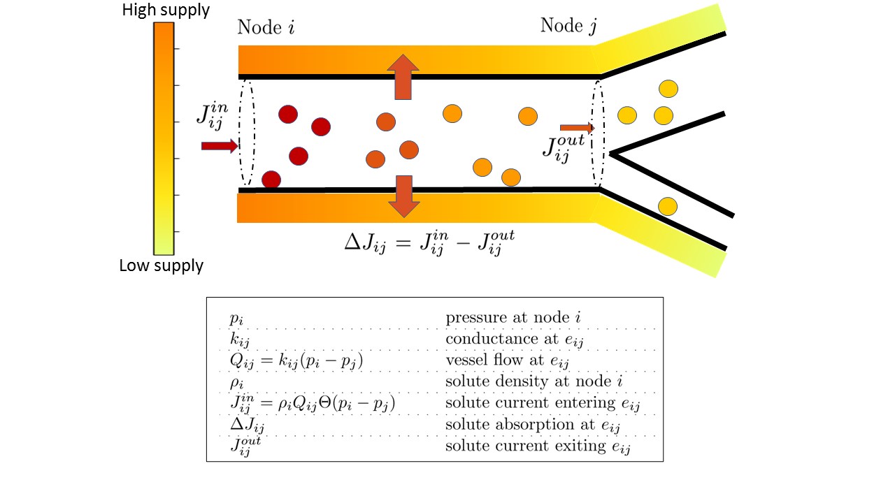
Figure 1: Nutrients transported through the vasculature. $J^{in}_{ij}=\rho_{i}Q_{ij}$ is the incoming nutrient current, $Q_{ij}$ is the fluid flow in the vessel and $\rho_{i}$ the nutrient density at node $i$ suspended to the flow. The color depicts the drop in the nutrient density between the input and output of each vessel due to the absorption of solutes.

Murray was the first one to mathematically cast vascular adaptation as a minimization problem of the energy dissipated by the flow. Most of the recent studies still focus on the optimization of transport cost subject to a material cost constraintKirkegaard and Sneppen (2020). In the absence of fluctuations, it was shown that minimum dissipation networks have a treelike topology and cannot maintain loops Bohn and Magnasco (2007); Kaiser et al. (2020). Other attempts managed to preserve loops by imposing uniformity in flow field, however this leads in a uniform conductance network that does not have any hierarchy Chang and Roper (2019) drastically increasing the transport costs.

Experimental evidence show that biological flow networks exhibit both hierarchy and loopy structure Roy et al. (2012), therefore suggesting the need for new optimization principles that go beyond dissipation and material cost Shweiki et al. (1992). Indeed, the main purpose of capillary networks is to efficiently supply tissues with nutrients such as oxygen, transported by the fluid. Details matter (where the tissue is, what the tissue function is), and uniformly distributing nutrients (equidistribution) is important as underfed areas will become hypoxic and eventually die. The importance of modeling certain aspects of vasculature design and its effects on flow and nutrient transport (e.g in the case of fetoplacental networks Erlich et al. (2019), the liver Kramer and Modes (2020), the kidneys Postnov et al. (2016), the torso and head Tekin et al. (2016) or brain microvasculature Meigel et al. (2019); Qi and Roper (2021)) has been long recognized by the community.

Equidistribution of load has been examined in vertex models where the radii of the supply vessels are constrained to be fixed but the vertices are allowed to move Gavrilchenko and Katifori (2021). However, solute perfusion networks have not been studied systematically from the vascular optimization perspective, in which each vessel adapts its diameter in order to regulate the nutrient supply, leading to hierarchical networks. This is crucial because often efficient nutrient perfusion is incompatible with network structures that minimize the cost of flow transport. This comes from the fact that in some systems the nutrients are distributed in a different manner compared to the flow. For instance, anisotropy in the distribution of nutrients occurs due to non newtonian rheology effects like plasma skimming. In other cases, distant vessels from the solute source (towards the venule side) are often under-supplied with oxygen. As a result, the network must readjust, often increasing the diameters of the vessels in the hypoxic areas in order to meet the metabolic demand Pries AR (1998).

In this work, we derive from first principles a local adaptation rule that optimizes nutrient transport. At first, we describe a model for nutrient absorption through the vessels of a flow network. Then, we propose an energy cost function that consists of a perfusion term, the energy dissipation to circulate the flow and the material cost. We derive a local information adaptation rule for the diameters of the network links that minimizes the cost function. The different terms of the cost function compete to produce a variety of complex network morphologies. We explore the phenotypic transitions between the under-supplied and over-supplied regime. Finally, we validate the optimization rule in the rat mesentery network and we provide evidence that uniform perfusion optimization explains the angio-adaptation in realistic networks.

Networks of uniform perfusion

We model the microcirculation as a network of $N_{e}$ linear fluidic resistors, connected at $N_{v}$ nodes. The link connecting nodes $i$ and $j$ corresponds to the vessel $e_{ij}$ of a specific conductance $k_{ij}$. In the vascular networks that we consider the Reynolds number is small, and the vessels are long compared to their diameter. In this regime the conductances of individual vessels can be approximated by Hagen–Poiseuille’s law $k_{ij}=\frac{\pi R_{ij}^{4}}{8\mu l_{ij}}$, where $R_{ij}$ is the radius of the vessel $e_{ij}$, $l_{ij}$ is its length and $\mu$ the blood viscosity. The viscosity does depend on the blood hematocrit and vessel diameter, but for the theoretical part of this work for simplicity we used the same average value for the entire network (see also Materials and Methods). Each vessel carries a current $Q_{ij}$. When $Q_{ij}>0$ the liquid flows from node $i$ to node $j$. The flow is conserved at every node $i$ in the network: $\sum_{j,\langle i,j\rangle=1}Q_{ij}=Q^{b}_{i}$, where the summation is over all nodes $j$ that are connected to node $i$. $Q^{b}_{i}$ is the external flow entering the node $i$ (or leaving it if $Q^{b}_{i}<0$). We define the weighted Laplacian matrix of the network $\mathcal{L}=D-A$, $D$ is the weighted degree matrix and $A$ the weighted adjacency matrix such that $A_{ij}=k_{ij}$. Calculating the pseudo-inverse of the Laplacian and using the boundary condition vector of the flow allow us to solve for the pressures $p_{i}$ for all the the nodes: $\vec{P}=\mathcal{L}^{-1}\vec{Q^{B}}$, where $\vec{P}$ and $\vec{Q^{B}}$ are $N_{v}\times 1$ vectors whose $i_{th}$ element is the pressure $p_{i}$ and net current $Q^{B}_{i}$ respectively ($Q^{B}_{i}$ is non zero only if node $i$ is boundary flow input or output). Using the pressures and the conductances we can solve for the flow of each segment $Q_{ij}=k_{ij}(p_{i}-p_{j})$.

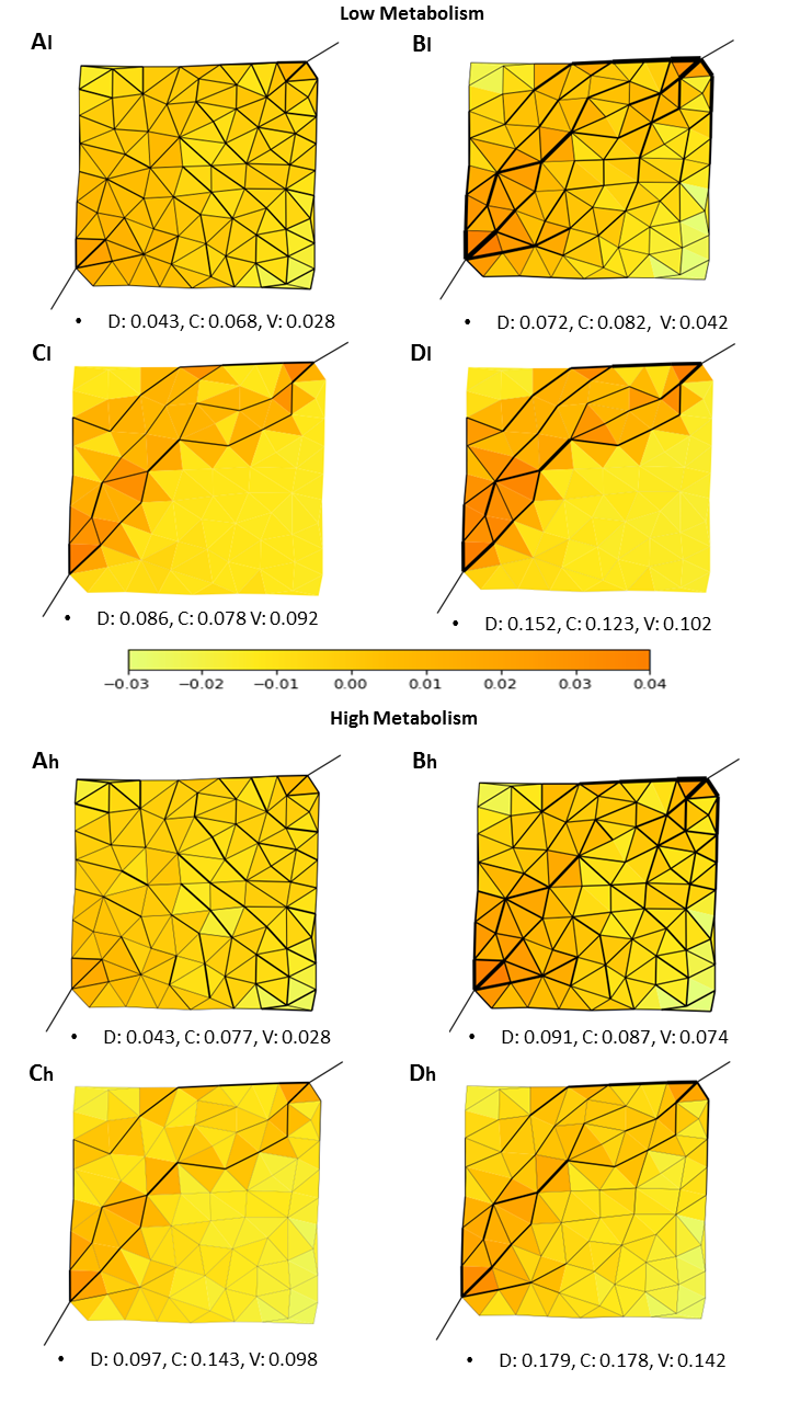
Figure 2: Optimized networks for different values of $\alpha,\omega$ and $\xi$. The edge width displayed is proportional to the conductance of the vessel and the color corresponds to the algebraic difference of the nutrient supply and the average absorption: $\Delta J-M$. When $\Delta J-M<0$ the vessels of the area are receiving less nutrients than the average metabolism $M$ of the whole network, and when $\Delta J-M>0$ they are oversupplied. The figures indexed as $l$ represent networks of low absorption rate while those indexed as $h$ have high absorption rate. Under each subplot are presented the values for the dissipation D, for the material cost C and for the nutrient absorption variance V.

To include the nutrients, we need to expand the model by introducing a nutrient density field $\rho_{i}$, defined at each node $i$ in the network. The nutrient density is transported by the flow so that the product of the density with the current $Q_{ij}$ gives the nutrient current $J_{ij}^{in}$ that enters from node $i$ and propagates downstream to node $j$ through the segment $e_{ij}$, as seen in Fig. 1:

$$J_{ij}^{in}=\rho_{i}Q_{ij}\Theta(p_{i}-p_{j}),$$ (1)

where $\Theta(p_{i}-p_{j})$ is the Heaviside function, necessary to ensure that the nutrient current has the same direction with the flow entering the segment $e_{ij}$. For simplicity in the results in the main text we ignore phase separation of red blood cells at the vessel bifurcations, however, the model is generalized to account for plasma skimming (see Materials and Methods 6). In perfusion networks, often nutrients diffuse through the vessels to the perivascular spaces. Therefore, the current $J_{ij}^{out}$ at the exit of the $e_{ij}$ vessel is reduced by $\Delta J_{ij}=J_{ij}^{in}-J_{ij}^{out}$. Here the ”in” and ”out” superscript is distinguishing the nutrient current entering and leaving the vessel respectively. In the case of nutrient diffusion across a long pipe, the absorption depends on the pipe characteristics such as the length, the diameter and the vessel’s absorption rate. Furthermore, the absorption depends on the fluid velocity and the density of solute. In this article we consider diffusion in low Reynolds number and we use the expression for nutrient absorption current as estimated analytically in Meigel and Alim (2018):

$$\Delta J_{ij}\approx\frac{1}{\frac{(\pi R_{ij})^{-1}Q_{ij}}{\xi l_{ij}}+1}\rho_{i}Q_{ij}=\frac{J_{ij}^{in}}{\tfrac{Q_{ij}(k_{ij})^{-1/4}}{\xi\lambda(l_{ij})^{5/4}}+1}$$ (2)

where $\xi$ is the absorption rate of the vessel $e_{ij}$ and $\lambda=(2^{3}\mu\pi^{3})^{1/4}$ is a constant characteristic of Poiseuille conductance. The dimensionless ratio $\frac{(\pi R_{ij})^{-1}Q_{ij}}{\xi l_{ij}}=\frac{t_{\text{d}}}{t_{\text{a}}}$ is the ratio of the time $t_{\text{d}}$ needed to diffuse radially through the cross section to the time $t_{\text{a}}$ needed to be advected out of the tube. Our method for direct calculation of the nutrient distribution can be applied to other absorption functions and as a result it is possible to be generalized to a broad array of systems.

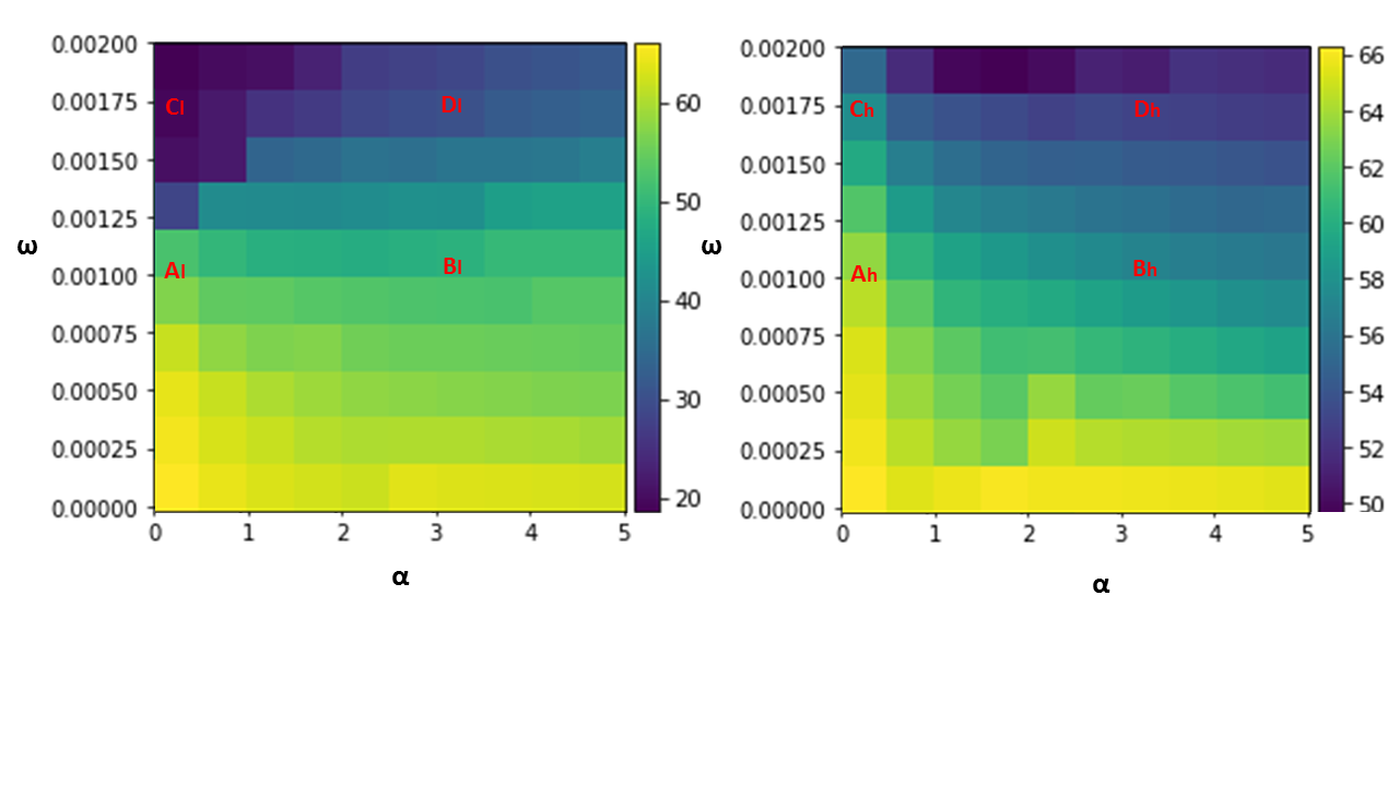
Figure 3: Heatmaps of the entropy of the optimized networks. On the left is the phase diagram for high absorption rate $\xi=0.3$. On the right is the diagram for low absorption rate $\xi=0.2$. The points marked on the phase diagrams represent the simulation results shown in Fig.2.

We proceed to calculate the nutrient distribution and absorption through the whole network. Nutrients enter the network through the $N_{B}$ source nodes. The density $\rho^{B}_{m}$ of the nutrients at every vertex $m$ that belongs to those boundary nodes is known. The particles are transported by the flow and propagate to the rest of the network. Despite the nutrient absorption at the edges, at each node there is conservation of nutrient mass so that the nutrient current entering the node $j$ equals the nutrient current exiting the node $j$, $\sum_{i}J^{out}_{ij}=\sum_{n}J^{in}_{jn}$.

Using the conservation of mass on the nodes, we can define an effective Laplacian matrix $\mathcal{L}_{\mathrm{eff}}$ which contains the nutrient absorption as a weight on the edges for a general absorption function $\Delta J$ (see Materials and Methods). Next, we obtain the nutrient field in the whole network by inverting $\mathcal{L}_{\mathrm{eff}}$ and multiplying with the boundary condition vector $\vec{J^{B}}$ that contains information of the nutrient external input on the nodes. The elements of $J^{B}_{i}$ are zero for internal nodes, and equal to $J^{B}_{m}=-\rho^{B}_{m}Q^{b}_{m}$, at each input boundary node $m$.

$$\vec{\rho}=\hat{\mathcal{L}}^{-1}_{\mathrm{eff}}\vec{J}^{B}.$$ (3)

Obtaining the nutrient field $\vec{\rho}$, we can calculate the nutrient absorption in each segment. The average absorption of the network is defined as $M=\sum_{i,j,\langle i,j\rangle=1}\frac{\Delta J_{ij}\Theta(p_{i}-p_{j})}{N_{e}}$. $M$ is considered as the characteristic metabolism of the network and depends on the graph structure and the absorption rate $\xi$ that is the same for all the vessels.

The adaptation rule for uniform perfusion networks

Our objective is to create networks that optimize a combination of cost functions: solute uniformity, dissipation, and material cost. This is achieved through a gradient descent algorithm that at each step modifies the hydraulic conductances of the vessels in such fashion so that the system moves closer to a minimum of an energy functional equal to a weighted sum of all three cost functions. The energy functional reads (see Supplement):

$$\begin{split}H(\{p_{i}\},\{k_{ij}\},\{\rho_{j}\})=\sum_{i,j,\langle i,j\rangle=1}\left(\Delta J_{ij}-M\right)^{2}\Theta(p_{i}-p_{j})&\\ +\omega\left[\sum_{i>j,\langle i,j\rangle=1}(\alpha k_{ij}(p_{i}-p_{j})^{2}+k_{ij}^{\gamma})\right]\end{split}$$ (4)

The energy explicitly depends on the pressures, conductances and the nutrient current densities written as ${p_{i}}$, $k_{ij}$, and $\rho_{j}$ respectively. However, the pressures and nutrient densities are an implicit function of the conductances, as they can be calculated using the constitutive relations 3 and Ohm’s law. The first sum is the variance of nutrient absorption in the system.

The second sum treats the mechanical energy of the system and consists of the dissipation power required to pump the fluid from the input to the output $\left(\sum_{i>j,\langle i,j\rangle=1}k_{ij}(p_{i}-p_{j})^{2}\right)$ and the material cost to maintain the vessels $\left(\sum_{i>j,\langle i,j\rangle=1}k_{ij}^{\gamma}\right)$ to the uniform perfusion term is quantified by the coefficient $\omega$. The coefficient $\alpha$ compares the dissipation to the material cost. In this work we consider $\gamma=\frac{1}{2}$ so that the material cost is proportional to the total volume of the system Chang and Roper (2019).

The optimized network is the one that corresponds to a local minimum of the energy 4. This minimum should satisfy $\nabla{H}=0$ with respect to all the independent variables. We propose that vascular systems adapt and remodel based on a local information adaptation rule that acts on each edge and that eventually leads the system to a steady state close to a local minimum of the energy 4. A similar idea in the absence of a perfusion term was presented in Hu and Cai (2013). To find an adaptive rule that results to an optimized steady state, i.e. a minimum of $H$, we perform a projected gradient descent. The $\{k_{ij}\}$ are treated as adiabatic variables Chang and Roper (2019), so at each step $n$ of the iterative process we update the conductances as $k^{n+1}_{ij}=k^{n}_{ij}+\delta k_{ij}$, where $\delta k_{ij}=-\nu\frac{\partial H}{\partial k_{ij}}$ and $\nu$ is the characteristic step size of the gradient descent algorithm Chang and Roper (2019). The rest of the variables of the system $(p_{i},\rho_{i})$ are assumed to vary more rapidly to remain at local equilibrium so $\frac{\partial H}{\partial p_{k}}=\frac{\partial H}{\partial\rho_{k}}=0$. At the end of each step, we update the rest of the variables $\left(p^{n+1}_{i},\rho^{n+1}_{i}\right)$ according to the constitutive relations and the new $\{k^{n+1}_{ij}\}$.

Using the above formulation we derive the following local information adaptation rule (see Supplement):

$$\begin{split}\frac{\partial k_{ij}}{\partial t}\sim-\frac{2Q_{ij}\rho_{i}\left(\frac{1}{4}\frac{Q_{ij}}{\xi l_{ij}^{5/4}k_{ij}^{1/4}}+1\right)}{k_{ij}\Big{(}\frac{Q_{ij}}{\xi l_{ij}^{5/4}k_{ij}^{1/4}}+1\Big{)}^{2}}\left[\frac{Q_{ij}\rho_{i}}{\frac{Q_{ij}}{\xi l_{ij}^{5/4}k_{ij}^{1/4}}+1}-M\right]\\ -\omega\left[-\alpha\frac{Q_{ij}^{2}}{k_{ij}^{2}}+\frac{1}{2}k_{ij}^{-\frac{1}{2}}\right].\end{split}$$ (5)

The growth or decrease in vessel $ij$ conductance depends only on the vessel flow $Q_{ij}$, local nutrient density $\rho_{i}$, and geometric parameters of the vessel. Implicitly, this adaptation function also depends on the boundary conditions of the flow and the nutrient density.

Results

To get an insight on the structure of the optimally perfused networks we use the proposed local adaptation relation 5 to numerically search for the minimum of the energy $H$. The simulations are performed on a triangular lattice of randomized edge lengths. We initialize the vessel conductances by assigning a value to each vessel drawn from a uniform distribution $[0.9,1.1]$. Then we initiate the adaptation process and at each step we update the conductances according to the energy gradient. For the simulations we use the non-dimensional energy 4 (see Supplement).

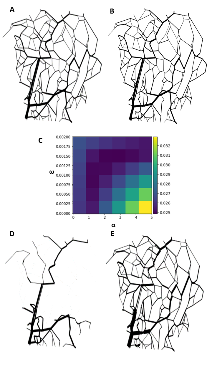
Figure 4: Mesentery vascular network simulation results for different optimization functions. A: The experimentally measured rat mesenteric network. B: Best fit simulation result for the energy functional including both the uniform perfusion term, the dissipation and the material cost for parameter values ($\omega=12*10^{-4}$, $\alpha=2.3$, $\xi=1.3*10^{-3}$). C: Heatmap of the relative error between the experiment and the simulation results. Networks that operate in the advective regime (low absorption rate $\xi$) show good agreement with the experimentally measured network: there is a range of parameters $\alpha,\omega$ for which the relative error is less than 2.5 %. D: Optimization result only for the minimization of dissipation without the uniform perfusion term. This network as expected does not preserve the topology of the experiment since loops vanish. E: Optimization only of the uniform perfusion term without dissipation and material cost. This network maintains the experimental topology however it does not preserve hierarchy, e.g. distant vessels with respect to the nutrient source have dilated diameters to increase their supply.

The adaptation process eventually leads to a minimization of the total energy $H$. During this process the uniform perfusion term and the dissipation compete to impose space filling and hierarchy respectively. In the absence of flow fluctuations for $\gamma<1$ loops are not stable Bohn and Magnasco (2007) when dissipation energy is minimized. However, here we demonstrate that it is possible for a network to maintain loops for stationary, non fluctuating flow when the target function to be optimized includes a term that minimizes uniform perfusion. The absorption rate $\xi$ affects the competition between the perfusion term and the mechanical costs changes, and as a result the network morphology. For high $\xi$ the network is organised in a space-filling, non-hierarchical mesh while for low $\xi$ the network becomes hierarchical. This behaviour is shown in Fig. 2. In the first set of panels $A_{l},B_{l},C_{l},D_{l}$ the absorption rate is low ($\xi=0.2$). For small absorption rate the network organises in long channels and the number of loops drastically decreases, optimizing the transport cost. For higher absorption rate $\xi=0.3$ in Fig. 2($C_{h}$) the network transitions from the advective regime to the diffusive regime and loops coexist with long channels. In this regime, uniform distribution of nutrients is prioritized while the transport cost is maintained relatively low. For very high absorption rate the average metabolism increases and the uniform perfusion term dominates. As a result the network is organized in a uniform grid and the vessels that are under-supplied tend to increase their cross sectional area.

In order to classify the spectrum of micro-vascular networks we use the entropy of the flow as an order parameter. Informational entropy measures the amount of uncertainty in a situation or system Ang and Jowitt (2005). For a water distribution network, the entropy $S$ represents the uncertainty faced by the water molecule as to which path it takes to go from the input source to the exit sink. The total entropy of the flow system is calculated as $S=\sum_{n=1}^{N_{v}}w_{n}S_{n}$, where $S_{n}$ is the entropy of node $n$ $S_{n}=-\sum_{n,j}P_{nj}\ln(P_{nj})$ for $Q_{nj}>0$ and $w_{n}=\frac{T_{n}}{T_{0}}$ is the the relative weight of node $n$, calculated as the ratio of the total outflow $T_{n}$ of the node $n$ to the the total supply $T_{0}$. Finally, here $P_{nj}=\frac{Q_{nj}}{T_{n}}$, is the probability that a molecule that arrives at $n$ will flow in the vessel $e_{nj}$.

The entropy of the optimized networks for a range of values of $\alpha$ and $\omega$, for low and high $\xi$ as shown in Fig. 3. The eight networks for low and high $\xi$ are displayed in Fig. 2 are labeled in the entropy heatmaps. Hierarchical networks, as for example ‘C_l’ exhibit lower entropy, as most of the loops disappear reducing the uncertainty in the possible flow paths. In this case, high $\omega$ means dissipation cost is prioritized to uniform perfusion. On the contrary networks in which uniform perfusion prevails, e.g. ‘A_h’ , have higher connectivity and as a result the multiplicity of paths is higher leading to higher entropy.

Uniform perfusion in the rat mesentery microvascular network

Structural adaptation of vascular beds involves responses not only to mechanical stimuli but also to the metabolic state of the tissue. In this section we show that the local adaptation rule of Eq. 5 that optimizes a linear combination of perfusion and mechanical cost is consistent with real vascular networks. To properly simulate perfusion and test the adaptive rule, data about the geometry (diameters and lengths of each segment), topology (connection matrix of vessel segments), and boundary conditions (volume flow rates, the discharge hematocrit in all vessel segments feeding the network and the volume flow rates for those segments leaving the network) are necessary. These data was provided for a 2-D section of the rat mesentery vascular network in Pries AR (1998). This network was supplied by arterioles with inner diameters of 30 $\mu m$ and drained by venules of 45 $\mu m$.

We first test the stability of the experimental network to an adaptation relation of the form 5. We start from the experimentally measured configuration of conductances and flows and we apply the adaptation algorithms for different sets of parameters $\{\alpha,\omega,\xi\}$.

The adaptation is terminated once the network stops evolving and ($\delta\kappa_{ij}$ drops below a certain threshold for every edge $e_{ij}$). Then we compare the final adapted radii $R_{n}^{sim}$ of each vessel $n$ with their initial, experimental values $R_{n}^{ex}$ and calculate the relative error: $\delta R=\frac{\sqrt{\sum_{n=1}^{N_{e}}\big{(}R_{n}^{ex}-R_{n}^{sim}\big{)}^{2}}}{\sum_{n=1}^{N_{e}}R_{n}^{ex}}$.

We find that there is set of coefficients for which the simulation result remains close to the experimental solution and that is $\omega=12*10^{-4}$, $\alpha=2.3$ and $\xi=1.3*10^{-3}$, with error $\delta R=1.6\%$. This implies that the experimental network is an equilibrium point of our optimization scheme. In Fig. 4A we present the experimental network and in Fig. 4B we plot the best fit result. The agreement between the two images suggests that the experimental vascular network is a local minimum for our energy functional, and stable under the adaptation rule. This adaptation result combines hierarchy and mesh structure. The network is operating at the advective regime because $\xi\ll 1$, and since the dissipation coefficient is large the transport of nutrients is more prioritised over the absorption Meigel et al. (2019). Nonetheless, the inclusion of the perfusion variance term in the cost function is crucial to maintain the loops and prevent distant vessels from vanishing Fig. 4D.That maintains the distribution of nutrients homogeneous.

This result is not due to fine tuning, and carefully selected values for $\alpha$, $\omega$ and $\xi$. As shown in Fig. 4C, there is a range of parameters $\alpha$, $\omega$ for which the steady state network is close to the experimental state with an error less than 3 %.

To further verify that the experimental state is indeed a minimum energy configuration of our model, we go beyond checking for stability and instead investigate if the adaptation algorithm would reproduce the network starting from a different, but nearby initial condition. For this, we perturb the initial experimental radii of order (80%) so that the disturbed diameter is: $\tilde{R}_{i}=R_{i}+\eta_{i}R_{i}$, where $\tilde{R}_{i}$ is the initial distribution and $\eta_{i}$ is a random variable sampled from $[-0.8,0.8]$, as seen in Fig. 5A, and use these as the initial diameters of the adaptation algorithm. For the adaptation process we choose in Fig. 5B we show the steady state network obtained by an adaptation process using the parameters $\alpha$, $\omega$, $\xi$ that best agree with the experimental data in the stability test.The steady state network recovers the experimental topology and conductance distribution. Under this adaptation rule the average difference from the experimental diameters decreased from (80%) to (20%). The rugged energy landscape of this energy functional results in the adaptation algorithm getting trapped in local minima. In the absence of any annealing type process, exactly reproducing the experimental state is unlikely.

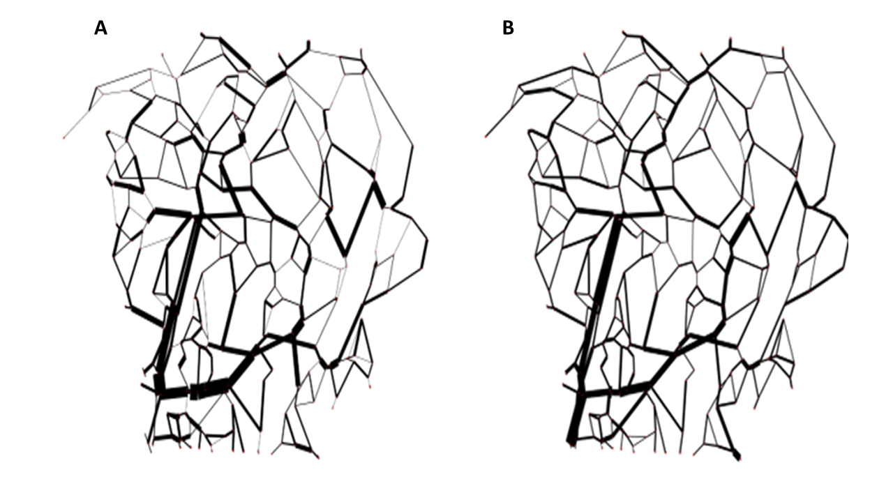
Figure 5: Mesentery vascular network with randomized initial vessel diameters. A: Randomized initial conditions. The added noise on the experimental diameters is 80% of their initial value. B: The optimized network ends in a minimum energy state that recovers the experimental distribution of experimental diameters within an error is $\delta R=20\%$. For the adaptation process we chose the set of coefficients $\omega,\ \alpha,\ \xi$ that produced the optimum network calculated at Fig. 4B.

Discussion

In this work we investigate how vascular networks remodel under a local information adaptation rule directly derived from optimization principles. Former studies that derive the local angioadaptation rules from optimization principles consider only the fluid flow in the adaptation process, and ignore the nutrient concentration. Either they minimize the flow dissipation cost Bohn and Magnasco (2007), Ronellenfitsch and Katifori (2016) or they impose uniform flow distribution Chang and Roper (2019), Epp et al. (2020). These optimization schemes produce either tree-like networks in the case of dissipation, with loops only appearing in the presence of fluctuations Ronellenfitsch and Katifori (2016), or a uniform grid in the case of uniform flow. However, often just the flow itself cannot capture the behaviour of the nutrients. In the microvasculature, nutrients typically diffuse to the tissue along the length of the vessels, and as a result one would typically expect some extent of nutrient deficit downstream, distally to network’s input. Moreover, when plasma skimming is present, the red blood cell concentration is no longer directly proportional to the plasma current Gould and Linninger (2015). Unlike prior studies, our optimization principle results in an adaptation rule that includes the effect of hypoxia-induced angiogenic factors. Pries and Secomb (2014).

To apply our system of adaptation equations iteratively required the solution of a system of flow equations that aimed to reproduce how nutrients are carried by the flow and how they diffuse through the vessels. We solve this system and obtain the nutrient field by inverting a sparse matrix instead of performing multiple iterations to propagate the solution node-wise starting from the input node to the exit (Materials and Methods). The computational efficiency of our method would permit generalization of our method to larger network systems.

Minimizing the variance of perfusion Adaptation, alongside the dissipation and material cost, can produce a spectrum of transport networks depending on the value of the constants $\alpha$, $\omega$ and $\xi$. This supports the alluring hypothesis that all the diversity of physiological vasculature can be produced by the same adaptation equation, and a handful of fitting constants. This diversity is produced by competition of the mechanical costs, which are optimized by a tree like architecture, and the uniform perfusion term Adaptation, which nudges the network to remain tightly meshed (Materials and Methods).

In general, perfusion networks can be roughly classified in two categories: advective and diffusive Meigel et al. (2019). The model in this work predicts a transition as we vary the absorption demand $\xi$. In the advective regime that appears for low $\xi$, the overall nutrient absorption is low, consistent with a low metabolism. In this scenario favors formation of hierarchical and long channels, as for the same parameters $\alpha$ and $\omega$ dissipation is relatively more costly than the perfusion variance term, which is smaller. For intermediate $\xi$, the metabolic demand is increased and therefore the network transitions to a regime in which perfusion becomes more important. In this case a mesh grid of small vessels is maintained, but can coexist with the formation of larger channels. If we further increase the absorption so that $\xi$ becomes large, uniformity is favored over hierarchy and the network transitions to a well-connected capillary bed. The system’s ability to maintain loops comes from the perfusion variance cost term Adaptation competing with the material cost (Materials and Methods).

The crossover between advection to diffusion can be successfully captured from the entropy of the flow, an order parameter that we use to quantify the structure of the various micro-circulation networks. Near the critical metabolism there is a discontinuous jump in the entropy while moving from lower values of absorption to higher values, as shown in Supplementary Fig 3. The flow entropy is an efficient parameter to capture the transition from a hierarchical to a uniform network while other parameters such as graph connectivity fail. For instance in Fig. 2 networks $B_{h}$ and $C_{h}$ have the same number of links however in $B_{h}$ the vessel conductances are of the same order of magnitude, while in $C_{h}$ there is coexistence of two vessel groups those that are forming long channels high in flow and those which form a uniform grid, the difference in their conductances is almost two orders of magnitude.

To test whether the optimization rule is consistent with experimentally obtained data, we apply the hemodynamic adaptation rule to the rat mesenteric vasculature. We show that minimizing the energy cost function 4 that accounts for uniform perfusion at the advective regime reproduces the mesenteric vasculature structure to a relatively high degree. Remarkably, the experimental architecture was captured only with the use of three fitting parameters $\{\xi,\omega,\alpha\}$, and for a broad range of values. Pries et al in Pries et al. (2003) manage to reproduce the mesentery structure with very high accuracy. However, in that work, the adaptation rule was ad-hoc, not directly connected or derived from optimization principles, and included 9 fitting parameters.

The adaptation model presented in our work is not necessarily complete: other mechanisms not included in the analysis may be relevant or even essential in the control of micro-vascular network structure. Specifically, highly metabolically active organs such as the brain, where fluctuations play an important role, may require additional elements in the model Blinder et al. (2013), or in the case of capillary beds, in which rheological effects of blood are more significant Chang and Roper (2019). Nonetheless, the theory developed here explains to a good degree the vascular structure of the mesentery and paves the way to include uniform perfusion of nutrients as dominant mechanism for angio-vascular adaptation. The model merits further experimental investigation, in other animal tissues and organs, and even plants, which have nutrient distributing flow networks. Furthermore, understanding how biological networks optimize transport can be educative in other fields of research and technology. For instance in the field of energy it could suggest new optimized designs of the channels of redox flow batteries or give new insights in the optimisation of supply distribution networks.

In the course of preparing this manuscript we became aware of related unpublished work by Kramer et al, concurrently posted on the Arxiv.

Appendix

A model for nutrient transport

In the results presented in this work, it is assumed that the nutrients at each junction are distributed proportionally to the flow. This implies that if a flow density $\rho_{o}$ enters a junction, the outgoing currents from that junction will carry the same nutrient density, and that the total amount of nutrients in each vessel will be proportional to the flow. However, often in micro-circulation the nutrients are not distributed proportionally to the flow: the daughter vessel with the larger diameter receives disproportionately more red blood cells. If at node ’$i$’ the nutrients are $\rho_{i}$, the nutrient density at the daughter vessels $\{ij\}$ that are supplied by i is determined by $\rho_{j}=\Phi_{ij}\rho_{i}$, where $\Phi_{ij}$ is coefficient equal to:

$$\Phi_{ij}=\left(\frac{Q_{ij}\Theta(p_{i}-p_{j})}{\left|\sum_{l,\langle l,i\rangle=1}{Q_{li}\Theta(p_{l}-p_{i})}\right|}\right)^{\eta}$$ (6)

The sum in the denominator represents the total incoming current to node $i$ and $\eta$ is the skimming exponent, a measure of the non linear splitting of the RBC’s at the bifurcations. For $\eta=0$ we have no skimming effect. For the human vasculature a reference value is $\eta=0.26$. For simplicity in our simulations we ignored the plasma skimming effect. Nevertheless the model is designed to account for it. It is worth mentioning that according to Pries et al. (1989) for diameters over 30 $\mu m$ the plasma phase separation effect is negligible for the rat mesentery network however in the work of Chang 10.1371/journal.pcbi.1005892. In the equations that follow, we present the most general model with $\eta\neq 0$.

The nutrient current, flowing from node $i$ to node $j$ reads:

$$J_{ij}^{in}=\rho_{i}Q_{ij}\Phi_{ij}\Theta(p_{i}-p_{j})$$ (7)

Nutrients like oxygen get absorbed as they are transported through the vessels so there is a drop between the incoming and exiting currents

$$\Delta J_{ij}=J_{ij}^{in}-J_{ij}^{out}$$ (8)

where $\Delta J_{ij}\approx\frac{\rho_{i}Q_{ij}}{\tfrac{Q_{ij}(k_{ij})^{-1/4}}{\xi\lambda(l_{ij})^{5/4}}+1}$ is the amount of nutrients that is being absorbed along the length of the vessel.

Summing 8 over the index $i$ we obtain:

$$\sum_{i}J^{in}_{ij}-\sum_{i}J^{out}_{ij}=\sum_{i}\Delta J_{ij}$$ (9)

Furthermore, we imply conservation of nutrient mass at each node so that the nutrient current entering the node $j$ equals the current exiting the node $j$ $\sum_{i}J^{out}_{ij}=\sum_{n}J^{in}_{jn}$. Then, Eq.  9 can be written as:

$$\begin{split}\sum_{i}\rho_{i}\Phi_{ij}Q_{ij}\Theta(p_{i}-p_{j})-\sum_{n}\rho_{j}\Phi_{jn}Q_{jn}\Theta(p_{i}-p_{j})&\\ =\sum_{i}A_{ij}\rho_{i}\Phi_{ij}Q_{ij}\Theta(p_{i}-p_{j}),\end{split}$$ (10)

where $A_{ij}=\frac{1}{\tfrac{Q_{ij}(k_{ij})^{-1/4}}{\xi\lambda(l_{ij})^{5/4}}+1}$. For simplicity, we define $B_{ij}\equiv(1-A_{ij})\Phi_{ij}Q_{ij}\Theta(p_{i}-p_{j})$ and $F_{ij}\equiv\Phi_{ij}Q_{ij}\Theta(p_{i}-p_{j})$, which simplifies Eq. 9 to $\sum_{i}\rho_{i}B_{ij}-\rho_{j}\sum_{k}F_{jk}$=0.

This final expression allows us to solve the system in matrix form. $Q_{ij}$ is a square matrix with dimension $N_{v}\times N_{v}$ containing the information of the currents, $A_{ij}$ is of same size but contains information about the loss among the different edges. $\Phi_{ij}$ is the matrix element that refers to the splitting law of nutrients at each bifurcation. Finally, $\rho_{i}$ is a vector element which corresponds to nutrient number at each node $i$ of the network. This is the variable that we want to solve for in the system.

The matrix form of the system becomes:

$$\left(\left(\widehat{\Phi}\widehat{Q}\right)^{T}-\widehat{D}\right)\vec{\rho}=\left(\widehat{A}\widehat{\Phi}\widehat{Q}\right)^{T}\vec{\rho}-\vec{\rho}^{B}\vec{S}.$$ (11)

Here $\hat{D}$ is a diagonal matrix that has the effect of a diode. It contains information about the direction of the nutrient current ensuring that we keep only the positive components, also it contains the weights for the case of nonlinear splitting of RBCs at the bifurcations.

$$\widehat{D}=\begin{bmatrix}\sum_{i}\Phi_{1i}Q_{1i}&0&...&0\\ 0&\sum_{n}\Phi_{2n}Q_{2n}&...&0\\ .&.&...&0\\ 0&0&...&\sum_{k}\Phi_{nk}Q_{nk}\end{bmatrix}$$

We can solve for $\vec{\rho}$ by imposing the boundary conditions on the density $\vec{\rho}^{B}$. For each boundary node belonging to the set of $n_{b}$ boundary nodes where current enters or leaves the system we introduce a pseudo node and we connect them with an edge. So the total number of nodes is now $\tilde{N}=(N_{v}+n_{b})$. We define the incoming nutrient current on the input node as $J^{B}_{m}=-\rho^{B}_{m}Q^{b}_{m}$. Then we write the transport equations in a compact form using the effective Laplacian matrix as defined below:

$$\left[\left(\widehat{I}-\widehat{B}^{T}\right)\left(\widehat{Q}\widehat{\Phi}\right)^{T}-\widehat{D}\right]\vec{\rho}=\vec{J}^{B},$$ (12)

$$\vec{\rho}=\hat{\mathcal{L}}^{-1}_{\mathrm{eff}}\vec{J}^{B},$$ (13)

where $I$ is the unitary $\tilde{N}\times\tilde{N}$ matrix. In order to invert the matrix expression in the brackets on the left side of the equation and to solve for all the values of $\rho_{i}$ we delete the columns and rows of the Laplacian that correspond to the boundary nodes.

Adaptation

At any local minimum of the system’s energy $H$, each of the partial derivatives must vanish. In order to solve the equation $\nabla{H}=0$ we perform gradient descent.

$$\begin{split}H{(\{p_{k}\},\{k_{kl}\},\{\rho_{k}\})}=\sum_{i,j,\langle i,j\rangle=1}\left(\Delta J_{ij}-M\right)^{2}\Theta(p_{i}-p_{j})&\\ +\omega\left[\sum_{i>j,\langle i,j\rangle=1}(\alpha k_{ij}(p_{i}-pj)^{2}+k_{ij}^{\gamma})-E_{0}\right]&\\ +\sum_{i}\mu_{k}\left(\sum_{\langle i,j\rangle=1}k_{ij}(p_{i}-p_{j})\right)\end{split}$$

$E_{0}$ can be considered as the initial energy of the system, the sum of the total dissipation and the total initial material cost. In the case of a constraint optimization problem $\omega$ can be interpreted as a Lagrange multiplier responsible to maintain the mechanical energy fixed. However, in our analysis while testing the experimental network we preferred not to add a ”hard” constraint for the total energy of the system. As a result $E_{0}=0$ and $\omega$ is only a coefficient regulating the relative strength of dissipation and material cost relatively to the uniform perfusion.

The Lagrange multipliers $\mu_{k}$, enforce conservation of flow at the Neumann vertices k in which there is external current source $q_{k}$. It is possible to insert directly the conservation of mass through the use of the graph Laplacian when calculating the flows therefore we ignore the last sum. The metabolism $M$ was interpreted as the intrinsic average absorption of the network and was controlled when varying the absorption rate $\xi$ of a single vessel: $M=\sum_{i,j,\langle i,j\rangle=1}\frac{\Delta J_{ij}\Theta(p_{i}-p_{j})}{N_{e}}$, where $N_{e}$ is the number of edges. It is worth mentioning that in other cases the metabolism can be inserted as an external parameter of the network.

While varying the metabolic demand we observed two distinct regimes, the advective and the diffusive Fig.4 ($C_{l}\ and\ C_{h}$) respectively. For the advection, $\xi_{l}\ll\xi_{crit}$ (see supplement) the absorption is independent of the flow velocity and nutrients are mainly transported not absorbed: $\Delta J_{ij}\approx\lambda l_{ij}^{5/4}\rho_{i}\xi k_{ij}^{1/4}$ in this regime long channels are formed to optimize transport cost. In the diffusive case, where $\xi_{h}>\xi_{crit}$ nutrient absorption prevails: $\Delta J_{ij}\approx\lambda\rho_{i}Q_{ij}$ a uniform grid is formed.

The various limits of the absorption rate dictate the scaling relation for the uniform perfusion $\sim$ $(\Delta J_{ij}-M)^{2}$. When the vessel $e_{ij}$ receives more nutrients than the metabolism $\Delta J_{ij}-M>0\$ or less $\Delta J_{ij}-M<0$ it is preferred to shrink or dilate respectively in order to minimize the variance. This effect, is evident especially in vessels that the flow supply is small so the dissipation term is negligible as seen in Fig.4. The transition of the network while varying the absorption rate $\xi$ for constant coefficients $\omega$ and $\alpha$ is discussed in detail in the Supplement. The transition is captured from the phase diagrams of flow entropy and dissipation cost in Fig.2 (Supplement).

Experimental data

In this work we use the data presented in Pries et al. (1989), Pries AR (1998) and other associated publications, generously shared by the authors. In this section we outline information related to this data, and our model validation.

The results presented in this work are from a microvascular network containing 913 vessel segments. The data set we were provided included the graph topology and geometry of the rat mesentery, accompanied by the diameters, flows and discharge hematocrit for every segment Pries et al. (1989). Our study required the network structure, the vessel diameters and only the flows boundary conditions and the discharge hematocrit at the feeding nodes from which we obtained the oxygen supply. The actual flows and solute distribution were calculated using the constitutive relations for the flow and nutrients, and found in agreement with the experimentally provided ones. In order to solve for the flows and the solute distribution, in principle one has to take into account the dependence of the relative viscosity on the discharge hematocrit and the diameters of the vessels, as described in Secomb and Pries (2013). However, we found that for the rat mesentery the corrections to the relative viscosity due to the discharge hematocrit are negligible. Therefore, in order to avoid the computational cost that is required to solve a nonlinear set of equations, we use the average viscosity over all the vessels of the network. For more details see Supplement.