Abstract.

Complex Event Recognition (CER) systems are a prominent technology for finding user-defined query patterns over large data streams in real time. CER query evaluation is known to be computationally challenging, since it requires maintaining a set of partial matches, and this set quickly grows super-linearly in the number of processed events. We present CORE, a novel COmplex event Recognition Engine that focuses on the efficient evaluation of a large class of complex event queries, including time windows as well as the partition-by event correlation operator. This engine uses a novel automaton-based evaluation algorithm that circumvents the super-linear partial match problem: under data complexity, it takes constant time per input event to maintain a data structure that compactly represents the set of partial matches and, once a match is found, the query results may be enumerated from the data structure with output-linear delay. We experimentally compare CORE against state-of-the-art CER systems on real-world data. We show that (1) CORE’s performance is stable with respect to both query and time window size, and (2) CORE outperforms the other systems by up to five orders of magnitude on different workloads.

PVLDB Reference Format:
PVLDB, 15(9): XXX-XXX, 2022.
doi:XX.XX/XXX.XX

PVLDB Artifact Availability:
The source code, data, and/or other artifacts have been made available at %leave␣empty␣if␣no␣availability␣url␣should␣be␣sethttps://github.com/CORE-cer.

1. Introduction

Complex Event Recognition (CER for short), also called Complex Event Processing, has emerged as a prominent technology for supporting streaming applications like maritime monitoring (Pitsikalis et al., 2019), network intrusion detection (Mukherjee et al., 1994), industrial control systems (Groover, 2007) and real-time analytics (Sahay and Ranjan, 2008). CER systems operate on high-velocity streams of primitive events and evaluate expressive event queries to detect complex events: collections of primitive events that satisfy some pattern. In particular, CER queries match incoming events on the basis of their content; where they occur in the input stream; and how this order relates to other events in the stream (Cugola and Margara, 2012b; Giatrakos et al., 2020; Alevizos et al., 2017).

CER systems hence aim to detect situations of interest, in the form of complex events, in order to give timely insights for implementing reactive responses to them when necessary. As such, they strive for low latency query evaluation. CER query evaluation, however, is known to be computationally challenging  (Agrawal et al., 2008; Mei and Madden, 2009; Cugola and Margara, 2012a; Zhang et al., 2014; Zhao et al., 2021; Zhao et al., 2020). Indeed, conceptually, evaluating a CER query requires maintaining or recomputing a set of partial matches, so that when a new event arrives all partial matches that—together with the newly arrived event–now form a complete answer can be found. Unfortunately, even for simple CER patterns, the set of partial matches quickly becomes polynomial in the number $N$ of previously processed events (or, when time windows are used, the number of events in the current window). Even worse, under the so-called skip-till-any-match selection strategy (Agrawal et al., 2008), queries that include the iteration operator may have sets of partial matches that grow exponentially in $N$ (Agrawal et al., 2008). As a result, the arrival of each new event requires a computation that is super-linear in $N$, which is incompatible with the small latency requirement.

In recognition of the computational challenge of CER query evaluation, a plethora of research has proposed innovative evaluation methods (Giatrakos et al., 2020; Cugola and Margara, 2012b; Artikis et al., 2017b). These methods range from proposing diverse execution models (Wu et al., 2006; Demers et al., 2006; Mei and Madden, 2009; Artikis et al., 2012), including cost-based database-style query optimizations to trade-off between materialization and lazy computation (Mei and Madden, 2009; Kolchinsky et al., 2015; Kolchinsky and Schuster, 2018); to focusing on specific query fragments (e.g., event selection policies (Agrawal et al., 2008)) that somewhat limit the super-linear partial match explosion; to using load shedding (Zhao et al., 2020) to obtain low latency at the expense of potentially missing matches; and to employing distributed computation (Cugola and Margara, 2012a; Mayer et al., 2017). All of these still suffer, however, from a processing overhead per event that is super-linear in $N$. As such, their scalability is limited to CER queries over a short time window, as we show in Section 5. Unfortunately, for applications such as maritime monitoring (Pitsikalis et al., 2019), network intrusion (Mukherjee et al., 1994) and fraud detection (Artikis et al., 2017a), long time windows are necessary and a solution based on new principles hence seems desirable.

In recent work (Grez et al., 2021, 2019), a subset of the authors have proposed a theoretical algorithm for evaluating CER queries that circumvents the super-linear partial match problem in theory: under data complexity the algorithm takes constant time per input event to maintain a data structure that compactly represents the set of partial and full matches in a size that is at most linear in $N$. Once a match is found, complex event(s) may be enumerated from the data structure with output-linear delay, meaning that the time required to output recognized complex event $C$ is linear in the size of $C$. This complexity is asymptotically optimal since any evaluation algorithm needs to at least inspect every input event and list the query answers.

Briefly, the evaluation algorithm consists of translating a CER query into a particular kind of automaton model, called a Complex Event Automaton (CEA). Given a CEA and an input event stream, the algorithm simulates the CEA on the stream, and records all CEA runs by means of a graph data structure. Interestingly, this graph succinctly encodes all the partial and complete matches. When a new event arrives, the graph can be updated in constant time to represent the new (partial) runs. Once a final state of the automaton is reached, a traversal over the graph allows to enumerate the complex events with output-linear delay.

To date, this approach to CER query evaluation has only been the subject of theoretical investigation. Because it is the only known algorithm that provably circumvents the super-linear partial match problem, however, the question is whether it can serve as the basis of a practical CER system. In this paper, we answer this question affirmatively by presenting CORE, a novel COmplex event Recognition Engine based on the principles of (Grez et al., 2021, 2019, 2020).

A key limitation of (Grez et al., 2021, 2019) that we need to resolve in designing CORE is that time windows are not supported in (Grez et al., 2021, 2019), neither semantically at the query language level, nor at the evaluation algorithm level. Indeed, the algorithm records all runs, no matter how long ago the run occurred in the stream and no matter whether the run still occurs in the current time window. As such, it also does not prune the graph to clear space for further processing, which quickly becomes a memory bottleneck. Another limitation is that the algorithm cannot deal with simple equijoins, such as requiring all matching events to have identical values in a particular attribute. Such equijoins are typically expressed by means of the so-called partition-by operator (Giatrakos et al., 2020). We lift both limitations in CORE.

Technically, to ensure that CER queries with time windows can still be processed in constant update per event and output-linear delay enumeration we need to be able to represent CEA runs in a ranked order fashion: during enumeration, runs that start later in the stream must be traversed before runs that start earlier, so that once a run does not satisfy a time window restriction all runs that succeed it in the ranked order will not satisfy the time window either, and can therefore be pruned. The challenge is to encode this ranking in the graph representation of runs while ensuring that we continue to be able to update it in constant time per new event. This requires a completely new kind of graph data structure for encoding runs, and a correspondingly new CEA evaluation algorithm. This new algorithm is compatible with the partition-by operator, as we will see. We stress that, by this new algorithm, the runtime of CORE’s complexity per event is independent of the number of partial matches, as well as the length of the time window being used. It therefore supports long time windows by design.

Contributions.

Our contributions are as follows.

(1) To be precise about the query language features supported by CORE’s evaluation algorithm, we formally introduce CEQL, a functional query language that focuses on recognizing complex events. It supports common event recognition operators including sequencing, disjunction, filtering, iteration, and projection (Grez et al., 2019, 2020, 2021), extended with partition-by, and time-windows. Other features considered in the literature that focus on processing of complex events, such as aggregation (Poppe et al., 2017b, 2019), integration of non-event data sources (Zhao et al., 2021), and parallel or distributed (Schultz-Møller et al., 2009; Pietzuch et al., 2003; Cugola and Margara, 2012a) execution are currently not supported by CEQL, and left for future work.

(2) We present an evaluation algorithm for CEQL that is based on entirely new evaluation algorithm for CEA that deals with time windows and partitioning, thereby lifting the limitations of (Grez et al., 2019, 2020, 2021).

(3) We show that the algorithm is practical. We implement it inside of CORE, and experimentally compare CORE against state-of-the-art CER engines on real-world data. Our experiments show that CORE’s performance is stable: the throughput is not affected by the size of the query or size of the time window. Furthermore, CORE outperforms existing systems by one to five orders of magnitude in throughput on different query workloads.

The structure of the paper is as follows. We finish this section by discussing further related work not already mentioned above. We continue by introducing CEQL in Section 2. We present the CEA computation model in Section 3. The algorithm and its data structures are described in Section 4, which also discusses implementation aspects of CORE. We dedicate Section 5 to experiments and conclude in Section 6.

Because of space limitations, certain details, formal statements and proofs are deferred to the Appendix.

SELECT * FROM Stock WHERE SELL as msft; SELL as intel; SELL as amzn FILTER msft[name="MSFT"] AND msft[price > 100] AND intel[name="INTC"] AND amzn[name="AMZN"] AND amzn[price < 2000]	SELECT b FROM Stock WHERE (BUY or SELL) as s; (BUY or SELL) as b PARTITION BY [name], [volume] WITHIN 1 minute	SELECT MAX * FROM Stock WHERE (BUY OR SELL) as low; (BUY OR SELL)+ as mid; (BUY OR SELL as) high FILTER low[price < 100] AND mid[price >= 100] AND mid[price <= 2000] AND high[price > 2000] PARTITION BY [name]
$(Q_{1})$	$(Q_{2})$	$(Q_{3})$

Figure 1. CEQL queries on a Stock stream.

Further Related Work

CER systems are usually divided into three approaches: automata-based, tree-based, and logic-based, with some systems (e.g., (Esp, [n.d.]; Cugola and Margara, 2010; Zhao et al., 2020)) being hybrids. We refer to recent surveys (Cugola and Margara, 2012b; Giatrakos et al., 2020; Alevizos et al., 2017; Artikis et al., 2017b) of the field for in-depth discussion of these classes of systems. CORE falls within the class of automata-based systems (Demers et al., 2006, 2005; Zhang et al., 2014; Agrawal et al., 2008; Wu et al., 2006; Schultz-Møller et al., 2009; Pietzuch et al., 2003; Cugola and Margara, 2010; Zhao et al., 2021; Poppe et al., 2019, 2017a, 2017b; Kolchinsky et al., 2015). These systems use automata as their underlying execution model. As already mentioned, these systems either materialize a super-linear number of partial matches, or recompute them on the fly. Conceptually, almost all of these works propose a method to reduce the materialization/recomputation cost by representing partial matches in a more compact manner. CORE is the first system to propose a representation of partial matches with formal, proven, and optimal performance guarantees: linear in the number of seen events, with constant update cost, and output-linear enumeration delay.

Tree- and logic-based systems (Mei and Madden, 2009; Liu et al., 2011; Esp, [n.d.]; Anicic et al., 2010; Artikis et al., 2014; Chesani et al., 2010; Kolchinsky and Schuster, 2018) typically evaluate queries by constructing and evaluating a tree of CER operators, much like relational database systems evaluate relational algebra queries. Cost models can be used to identify efficient trees, and stream characteristics monitored to re-optimize trees during processing when necessary (Kolchinsky and Schuster, 2018). These evaluation trees do no have the formal, optimal performance guarantees offered by CORE.

Query evaluation with bounded delay has been extensively studied for relational database queries (Segoufin, 2013; Bagan et al., 2007; Idris et al., 2020; Berkholz et al., 2017, 2017; Carmeli and Kröll, 2021), where it forms an attractive evaluation method, especially when query output risks being much bigger than the size of the input. CORE applies this methodology to the CER domain which differs from the relational setting in the choice of query operators, in particular the presence of operators like sequencing and Kleene star (iteration). In this respect, CORE’s evaluation algorithm is closer the work on query evaluation with bounded delay over words and trees (Florenzano et al., 2020; Amarilli et al., 2021, 2017, 2019). Those works, however, do not consider enumeration with time window constraints as we do here.

2. CEQL syntax and semantics

CORE’s query language is similar in spirit to existing languages for expressing CER queries (see, e.g., (Cugola and Margara, 2012b; Giatrakos et al., 2020; Alevizos et al., 2017) for a language survey). In particular, CORE shares with these languages a common set of operators for expressing CER patterns, including, for example sequencing, disjunction, iteration (a.k.a. Kleene closure), and filtering, among others (Giatrakos et al., 2020; Alevizos et al., 2017). While hence conceptually similar, it is important to note that existing system implementations and their evaluation algorithms differ in (1) the exact set of operators supported, (2) how these operators can be composed, and (3) even in the semantics ascribed to operators. Given these sometimes subtle (semantic) differences, we wish to be unambiguous about the class of queries supported by CORE’s evaluation algorithm. In this section, we therefore formally define the syntax and semantics of CEQL, the query language that is fully implemented by CORE.

CEQL is based on Complex Event Logic (CEL for short)—a formal logic that is built from the above-mentioned common operators without restrictions on composability, and whose expressiveness and complexity have been studied in (Grez et al., 2019, 2020, 2021). CEQL extends CEL by adding support for time windows as well as the partition-by event correlation operator. We first introduce CEQL by means of examples, and then proceed with the formal syntax and semantics.

2.1. CEQL by example

Consider that we have a stream Stock that is emitting BUY and SELL events of particular stocks. The events carry the stock name, the volume bought or sold, the price, and a timestamp. Suppose that we are interested in all triples of SELL events where the first is a sale of Microsoft over 100 USD, the second is a sale of Intel (of any price), and the third is a sale of Amazon below 2000 USD. Query $Q_{1}$ in Figure 1 expresses this in CEQL. In $Q_{1}$, the FROM clause indicates the streams to read events from, while the WHERE clause indicates the pattern of atomic events that need to be matched in the stream. This can be any unary Complex Event Logic (CEL) expression (Grez et al., 2021). In $Q_{1}$, the CEL expression

SELL as msft; SELL as intel; SELL as amzn

indicates that we wish to see three SELL events and that we will refer to the first, second and third events by means of the variables msft, intel and amzn, respectively. In particular, the semicolon operator (;) indicates sequencing among events. Sequencing in CORE is non-contiguous. As such, the msft event needs not be followed immediately by the intel event—there may be other events in between, and similarly for amzn. The FILTER clause requires the msft event to have MSFT in its name attribute, and a price above 100. It makes similar requirements on the intel and amzn events.

The conditions in a CEQL FILTER clause can only express predicates on single events. Correlation among events, in the form of equi-joins, is supported in CEQL by the PARTITION BY clause. This feature is illustrated by query $Q_{2}$ in Figure 1, which detects all pairs of BUY or SELL events of the same stock and the same volume. In particular, there, the PARTITION BY clause requests that all matched events have the same values in the name and volume attributes. The WITHIN clause specifies that the matched pattern must be detected within 1 minute. In CORE, each event is assigned the time at which it arrives to the system, so we do not assume that events include a special attribute representing time, as some other systems do. Finally, the SELECT clause ensures that, from the matched pair of events, only the event in variable b is returned.

In general, the pattern specified in the WHERE clause in a CEQL query may include other operators such as disjunction (denoted $~{}\mathtt{OR}~{}$​) and iteration (also known as Kleene closure, denoted +). These may be freely nested in the WHERE clause. Query $Q_{2}$ illustrates the use of disjunction. Query $Q_{3}$ illustrates the use of iteration. In $Q_{3}$, 100 and 2000 are two values representing a lower and upper limit price, respectively. $Q_{3}$ looks for an upward trend: a sequence of BUY or SELL events pertaining to the same stock symbol where the sale price is initially below 100 (captured by the low variable), then between 100 and 2000 (captured by mid), then above 2000 (high). Importantly, because of the Kleene closure iteration operator, variable mid captures all sales of the stock in the $[\textsf{100},\textsf{2000}]$ price range in such a trend. The MAX operator in the SELECT clause is an example of a selection strategy (Agrawal et al., 2008; Giatrakos et al., 2020; Grez et al., 2021): it ensures that within a trend mid is bound to a maximal sequence of events in the $[\textsf{100},\textsf{2000}]$ price range. If this policy were not specified, CEQL would adopt the skip-till-any-match policy (Agrawal et al., 2008; Giatrakos et al., 2020) by default, which also returns complex events with mid containing only subsets of this maximal sequences.

2.2. CEQL syntax and semantics

We start by defining CORE’s event model.

Events, complex events, and valuations.

We assume given a set of event types $\mathbf{T}$ (consisting, e.g., of the event types BUY and SELL in our running example), a set of attribute names $\mathbf{A}$ (e.g., name, price, etc) and a set of data values $\mathbf{D}$ (e.g. integers, strings, etc.). A data-tuple $t$ is a partial mapping that maps attribute names from $\mathbf{A}$ to data values in $\mathbf{D}$. Each data-tuple is associated to an event type. We denote by $t(a)\in\mathbf{D}$ the value of the attribute $a\in\mathbf{A}$ assigned by $t$, and by $t(\operatorname{type})\in\mathbf{T}$ the event type of $t$. If $t$ is not defined on attribute $a$, then we write $t(a)=\texttt{NULL}$.

A stream is a possibly infinite sequence $S=t_{0}t_{1}t_{2}\ldots$ of data-tuples. Given a set $D\subseteq\mathbb{N}$, we define the set of data tuples $S[D]=\{t_{i}\mid i\in D\}$. A complex event is a pair $C=([i,j],D)$ where $i\leq j\in\mathbb{N}$ and $D$ is a subset of $\{i,\ldots,j\}$. Intuitively, given a stream $S=t_{0}t_{1}\ldots$ the interval $[i,j]$ of $C$ represents the subsequence $t_{i}t_{i+1}\ldots t_{j}$ of $S$ where the complex event $C$ happens and $S[D]$ represents the data-tuples from $S$ that are relevant for $C$. We write $C(\operatorname{time})$ to denote the time-interval $[i,j]$, and $C(\operatorname{start})$ and $C(\operatorname{end})$ for $i$ and $j$, respectively. Furthermore, we write $C(\operatorname{data})$ to denote the set $D$.

To define the semantics of CEQL, we will also need the following notion. Let $\mathbf{X}$ be a set of variables, which includes all event types, $\mathbf{T}\subseteq\mathbf{X}$. A valuation is a pair $V=([i,j],\mu)$ with $[i,j]$ a time interval as above and $\mu$ a mapping that assigns subsets of $\{i,\ldots,j\}$ to variables in $\mathbf{X}$. Similar to complex events, we write $V(\operatorname{time})$, $V(\operatorname{start})$, and $V(\operatorname{end})$ for $[i,j]$, $i$, and $j$, respectively, and $V(X)$ for the subset of $\{i,\ldots,j\}$ assigned to $X\in\mathbf{X}$ by $\mu$.

We write $C_{V}$ for the complex event that is obtained from valuation $V$ by forgetting the variables in $V$, and retaining only its positions: $C_{V}(\operatorname{time})=V(\operatorname{time})$ and $C_{V}(\operatorname{data})=\bigcup_{X\in\mathbf{X}}V(X)$. The semantics of CEQL will be defined in terms of valuations, which are subsequently transformed into complex events in this manner.

Predicates

A (unary) predicate is a possibly infinite set $P$ of data-tuples. For example, $P$ could be the set of all tuples $t$ such that $t(\mathsf{price})\geq 100$. A data-tuple $t$ satisfies predicate $P$, denoted $t\models P$, if, and only if, $t\in P$. We generalize this definition from data-tuples to sets by taking a “for all” extension: a set of data-tuples $T$ satisfies $P$, denoted by $T\models P$, if, and only if, $t\models P$ for all $t\in T$.

CEQL.

Syntactically, a CEQL query has the form:

SELECT	[selection-strategy] $<\text{list-of-variables}>$
FROM	$<\text{list-of-streams}>$
WHERE	$<\text{CEL-formula}>$
[PARTITION BY	$<\text{list-of-attributes}>$]
[WITHIN	$<\text{time-value}>$]

Specifically, the WHERE clause consists of a formula in Complex Event Logic (CEL) (Grez et al., 2021), whose abstract syntax is given by the following grammar:

$$\varphi:=R\mid\varphi~{}\operatorname{AS}~{}X\mid\varphi~{}\mathtt{FILTER}~{}X\texttt{[}P\texttt{]}\mid\varphi~{}\mathtt{OR}~{}\varphi\mid\varphi\,;\,\varphi\mid\varphi+\mid~{}\pi_{L}~{}(\varphi).$$

In this grammar, $R$ is a event type in $\mathbf{T}$, $X$ is a variable in $\mathbf{X}$, $P$ is a predicate, and $L$ is a subset of variables in $\mathbf{X}$.

The semantics of CEQL is now as follows. Conceptually, a CEQL query first evaluates its FROM clause, then its PARTITION BY clause, and subsequently its WHERE, SELECT, and WITHIN clauses (in that order). The FROM clause merely specifies the list of streams registered to the system from which events should be inspected. All these streams are logically merged into a single stream $S$ that is processed by the subsequent clauses. The PARTITION BY clause, if present, logically partitions this stream into multiple substreams $S_{1},S_{2},\dots$, and executes the WHERE-SELECT-WITHIN clauses on each substream separately. The union of the outputs generated for each substream constitute the final output. Concretely, every $S_{i}$ is a maximal subsequence of $S$ such that for every pair of tuples $t$ and $t^{\prime}$ occurring in $S_{i}$, and for every attribute $a$ mentioned in the PARTITION BY clause, it holds that $t(a)\not=\texttt{NULL}$, $t^{\prime}(a)\not=\texttt{NULL}$, and $t(a)=t^{\prime}(a)$. As such, all tuples in $S_{i}$ share the same value in every attribute of the PARTITION BY clause.

The semantics of the WHERE-SELECT-WITHIN clauses is as follows. CEQL’s WHERE clause is derived from the semantics of CEL , which is inductively defined in Table 2. Concretely, given a stream $S=t_{0}t_{1}t_{2}\dots$ (or one of the substreams $S_{i}$ if the query has a PARTITION BY clause), a CEL formula $\varphi$ evaluates to a set of valuations, denoted ${\llceil{\varphi}\rrfloor}(S)$. The base case is when $\varphi$ is an event type $R$. In that case ${\llceil{\varphi}\rrfloor}(S)$ contains all valuations whose time-interval is a single position $i$, such that the data-tuple $t_{i}$ at position $i$ in $S$ is of type $R$. Furthermore, the valuation is such that variable $R$ (recall that $\mathbf{T}\subseteq\mathbf{X}$) stores only position $i$ and all other variables are empty. The $\operatorname{AS}$ clause is a variable assignment that takes an existing valuation $V\in{\llceil{\varphi}\rrfloor}(S)$ and extends it by gathering all positions $\cup_{Y}V(Y)$ in variable $X$, keeping all other variables as in $V$. The filter clause $\mathtt{FILTER}~{}X\texttt{[}P\texttt{]}$ retains only those valuations for which the content of variable $X$ satisfies predicate $P$, and the $\mathtt{OR}$ clause takes the union of two sets of valuations. The sequencing operator uses the time-interval for capturing all pairs of valuations in which the first is chronologically followed by the second. Specifically, ${\llceil{\varphi_{1}\,;\,\varphi_{2}}\rrfloor}(S)$ takes $V_{1}\in{\llceil{\varphi_{1}}\rrfloor}(S)$ and $V_{2}\in{\llceil{\varphi_{2}}\rrfloor}(S)$ such that $V_{2}$ is after $V_{1}$ (i.e., $V_{1}(\operatorname{end})<V_{2}(\operatorname{start})$) and joins them into one valuation $V$, where the time interval is given by the start of $V_{1}$ and the end of $V_{2}$. The semantics of iteration $\varphi+$ is defined as the application of sequencing (;) one or more times over the same formula. The projection $~{}\pi_{L}~{}$ modifies valuations by setting all variables that are not in $L$ to empty.

$${\llceil{R}\rrfloor}(S) \ =\ \{V\ \mid\!\!\begin{array}[t]{l}V(\operatorname{time})=[i,i]\ \wedge\ t_{i}(\operatorname{type})=R\\ \wedge\ \ V(R)=\{i\}\ \wedge\ \forall X\neq R.\ V(X)=\emptyset\ \}\end{array}$$

$${\llceil{\varphi~{}\operatorname{AS}~{}X}\rrfloor}(S) \ =\ \{V\ \mid\!\!\begin{array}[t]{l}\exists\ V^{\prime}\in{\llceil{\varphi}\rrfloor}(S).\ \ V(\operatorname{time})=V^{\prime}(\operatorname{time})\\ \wedge\ \ V(X)=\cup_{Y}V^{\prime}(Y)\\ \wedge\ \ \forall Z\neq X.\ V(Z)=V^{\prime}(Z)\ \}\end{array}$$

$${\llceil{\varphi~{}\mathtt{FILTER}~{}X\texttt{[}P\texttt{]}}\rrfloor}(S) \ =\ \{V\ \mid\ V\in{\llceil{\varphi}\rrfloor}(S)\wedge V(X)\models P\ \}$$

$${\llceil{\varphi_{1}~{}\mathtt{OR}~{}\varphi_{2}}\rrfloor}(S) \ =\ {\llceil{\varphi_{1}}\rrfloor}(S)\ \cup\ {\llceil{\varphi_{2}}\rrfloor}(S)$$

$${\llceil{\varphi_{1}\,;\,\varphi_{2}}\rrfloor}(S) \ =\ \{V\ \mid\!\!\begin{array}[t]{l}\exists\ V_{1}\in{\llceil{\varphi_{1}}\rrfloor}(S),V_{2}\in{\llceil{\varphi_{2}}\rrfloor}(S).\\ V_{1}(\operatorname{end})<V_{2}(\operatorname{start})\\ \wedge\ \ V(\operatorname{time})=[V_{1}(\operatorname{start}),V_{2}(\operatorname{end})]\\ \wedge\ \ \forall X.\ V(X)=V_{1}(X)\cup V_{2}(X)\ \}\end{array}$$

$${\llceil{\varphi+}\rrfloor}(S) \ =\ {\llceil{\varphi}\rrfloor}(S)\ \cup\ {\llceil{\varphi\,;\,\varphi+}\rrfloor}(S)$$

$${\llceil{~{}\pi_{L}~{}\!(\varphi)}\rrfloor}(S) \ =\ \{V\ \mid\!\!\begin{array}[t]{l}\exists\ V^{\prime}\in{\llceil{\varphi}\rrfloor}(S).\ V(\operatorname{time})=V^{\prime}(\operatorname{time})\\ \wedge\ \forall X\in L.\ V(X)=V^{\prime}(X)\\ \wedge\ \ \forall X\notin L.\ V(X)=\emptyset\}\end{array}$$

Figure 2. The semantics of a CEL formulas.

The WHERE part of a CEQL query hence returns a set of valuations when evaluated over a stream. The SELECT clause, if it does not mention a selection strategy, corresponds to a projection in CEL, and hence operates on this set accordingly. If it does specify a selection strategy, then a CEL projection is applied, followed by removing certain valuations from the set. We refer the interested reader to (Grez et al., 2021) for a definition and discussion of selection strategies. Finally, if $\epsilon$ is a time-interval, then the WITHIN clause operate on the resulting set of valuations as follows:

$${\llceil{\varphi~{}\mathtt{WITHIN}~{}\epsilon}\rrfloor}(S) \ =\ \{V\in{\llceil{\varphi}\rrfloor}(S)\mid V(\operatorname{end})-V(\operatorname{start})\leq\epsilon\}.$$

Complex Event Semantics.

The semantics defined above is one where CEL and CEQL queries return valuations. In CER systems, it is customary, however, to return complex events instead. The complex event semantics of CEL and CEQL is obtained by first evaluating the query under the valuation semantics, and then removing variables altogether. That is, if $\varphi$ is a CEL formula or CEQL query, its complex event semantics ${\llbracket{}{\varphi}\rrbracket}(S)$ is defined by ${\llbracket{}{\varphi}\rrbracket}(S):=\{C_{V}\mid V\in{\llceil{\varphi}\rrfloor}(S)\}.$ For the rest of this paper, we will be interested in efficiently computing the complex event semantics ${\llbracket{}{\varphi}\rrbracket}(S)$. We stress, however, that our techniques can be extended to also efficiently compute the valuation semantics instead.

3. Query compilation

At the heart of evaluating a CEQL query lies the problem of evaluating the query’s SELECT-WHERE-WITHIN clauses on either a single stream, or multiple different substreams thereof (for a query with PARTITION BY). In this section and the next, we discuss how to do so efficiently, focusing on evaluation over a single stream. To this end, let $Q$ be a CEQL query without PARTITION BY and with only one stream mentioned in the FROM clause.

In CORE we first compile the SELECT-WHERE part of $Q$ into a Complex Event Automaton (CEA for short) (Grez et al., 2019, 2021), which is a form of finite state automaton that produces complex events. CORE’s evaluation algorithm is then defined in terms of CEA: it takes as input a CEA $\mathcal{A}$, the (optional) time window $\epsilon$ specified in the WITHIN clause of $Q$, and a stream $S$, and uses this to compute ${\llbracket{}{Q}\rrbracket}(S)$. This evaluation algorithm is described in Section 4. Here, we introduce CEA.

Roughly speaking, a CEA is similar to a standard finite state automaton. The difference is that a standard finite state automaton processes finite strings and also has transitions of the form $p\raisebox{-1.0pt}[10.0pt][0.0pt]{$\overset{\sigma}{\underset{}{\raisebox{0.0pt}[3.0pt][0.0pt]{$\relbar\mspace{-8.0mu}\longrightarrow$}}}$}q$ with $q,p$ states and $\sigma$ a symbol from some finite alphabet, whereas a CEA processes possibly unbounded streams of data-tuples and has transitions of the form $p\raisebox{-1.0pt}[10.0pt][0.0pt]{$\overset{P/m}{\underset{}{\raisebox{0.0pt}[3.0pt][0.0pt]{$\relbar\mspace{-8.0mu}\longrightarrow$}}}$}q$ with $p$ and $q$ states, $P$ a predicate and $m$ an action, which can be marking ($\bullet$) or unmarking ($\circ$). The semantics of such a transition $p\raisebox{-1.0pt}[10.0pt][0.0pt]{$\overset{P/m}{\underset{}{\raisebox{0.0pt}[3.0pt][0.0pt]{$\relbar\mspace{-8.0mu}\longrightarrow$}}}$}q$ is that, when a new tuple $t$ arrives in the stream and the CEA is in state $p$, if $t$ satisfies $P$ then the CEA moves to state $q$ and applies the action $m$: if $m$ is a marking action then the event $t$ will be part of the output complex event once a final state is reached, otherwise it will not.

Figure 3. A CEA representing $Q_{1}$ from Figure 1 and some of its runs on an example stream.

Example 0.

In Figure 3 we show a CEA $\mathcal{A}$ that represents query $Q_{1}$ from Figure 1. There, we depict predicates by listing, in array notation, the event type, the requested value of the name attribute, and the constraint on the price attribute. The initial state is $q_{1}$ and there is only one final state: $q_{4}$. The figure also shows an example stream $S$, and several runs of $\mathcal{A}$ on $S$. Every run shown is accepting (i.e., ends in an accepting state of the automaton), and as such returns a complex event. The time of this complex event is the interval $[i,j]$ with $i$ the position where the run starts, and $j$ the position where the run ends. The data of this complex event consists of all positions marked by the run. For example, the complex event $C_{1}$ output by run $1$ is $([0,4],\{0,2,4\})$; the complex event $C_{2}$ output by run $2$ is $([0,6],\{0,2,6\})$, and so on.

Formally, a Complex Event Automaton (CEA) is a tuple $\mathcal{A}=(Q,\Delta,q_{0},F)$ where $Q$ is a finite set of states, $\Delta\subseteq Q\times\mathbf{P}\times\{\bullet,\circ\}\times(Q\setminus\{q_{0}\})$ is a finite transition relation, $q_{0}\in Q$ is the initial state, and $F\subseteq Q$ is the set of final states. We will denote transitions in $\Delta$ by $q\raisebox{-1.0pt}[10.0pt][0.0pt]{$\overset{P/m}{\underset{}{\raisebox{0.0pt}[3.0pt][0.0pt]{$\relbar\mspace{-8.0mu}\longrightarrow$}}}$}q^{\prime}$. A run of $\mathcal{A}$ over stream $S$ from positions $i$ to $j$ is a sequence $\rho\ :=\ q_{i}\,\raisebox{-1.0pt}[10.0pt][0.0pt]{$\overset{P_{i}/m_{i}}{\underset{}{\raisebox{0.0pt}[3.0pt][0.0pt]{$\relbar\mspace{-8.0mu}\longrightarrow$}}}$}\,q_{i+1}\,\raisebox{-1.0pt}[10.0pt][0.0pt]{$\overset{P_{i+1}/m_{i+1}}{\underset{}{\raisebox{0.0pt}[3.0pt][0.0pt]{$\relbar\mspace{-8.0mu}\longrightarrow$}}}$}\,\ldots\,\raisebox{-1.0pt}[10.0pt][0.0pt]{$\overset{P_{j}/m_{j}}{\underset{}{\raisebox{0.0pt}[3.0pt][0.0pt]{$\relbar\mspace{-8.0mu}\longrightarrow$}}}$}\,q_{j+1}$ such that $q_{i}$ is the initial state of $\mathcal{A}$ and for every $k\in[i,j]$ it holds that $q_{k}\raisebox{-1.0pt}[10.0pt][0.0pt]{$\overset{P_{k/m_{k}}}{\underset{}{\raisebox{0.0pt}[3.0pt][0.0pt]{$\relbar\mspace{-8.0mu}\longrightarrow$}}}$}q_{k+1}\in\Delta$ and $t_{k}\models P_{k}$. A run $\rho$ is accepting if $q_{j+1}\in F$. An accepting run $\rho$ of $\mathcal{A}$ over $S$ from $i$ to $j$ naturally defines the complex event $C_{\rho}\ :=\ ([i,j],\{k\mid i\leq k\leq j\wedge m_{k}=\bullet\}).$ If position $i$ and $j$ are clear from the context, we say that $\rho$ is a run of $\mathcal{A}$ over $S$. Finally, we define the semantics of $\mathcal{A}$ over a stream $S$ as ${\llbracket{}{\mathcal{A}}\rrbracket}(S):=\{C_{\rho}\mid\text{$\rho$ is an accepting run of $\mathcal{A}$ over $S$}\}.$

We note that in this paper, because we consider complex events with time intervals, a run may start at an arbitrary position $i$ in the stream, which differs from the semantics of CEA considered in (Grez et al., 2019, 2021) where complex events do not have time intervals and runs always start at the beginning of the stream. It is also important to note that in the definition above no transition can re-enter the initial state $q_{0}$; this will be important for defining the time-interval of the output complex events in Section 4. This requirement on the initial state is without loss of generality, since any incoming transitions into the initial state $q_{0}$ may be removed without modifying semantics by making a copy $q^{\prime}_{0}$ of $q_{0}$ (also copying its outgoing transitions) and rewrite any transition into $q_{0}$ to go to $q^{\prime}_{0}$ instead.

The usefulness of CEA comes from the fact that CEL can be translated into CEA (Grez et al., 2019, 2021). Because the SELECT-WHERE part of a CEQL query is in essence a CEL formula, this reduces the evaluation problem of the SELECT-WHERE-WITHIN part of CEQL query into the evaluation problem for CEA, in the following sense.

Theorem 2.

For every CEL formula $\varphi$ we can construct a CEA $\mathcal{A}$ of size linear in $\varphi$ such that for every $\epsilon$:

$${\llbracket{}{\varphi~{}\mathtt{WITHIN}~{}\epsilon}\rrbracket}(S)\ =\ \{C\mid C\in{\llbracket{}{\mathcal{A}}\rrbracket}(S)\wedge C(\operatorname{end})-C(\operatorname{start})\leq\epsilon\}.$$

Our evaluation algorithm will compute the right-hand side in this equation. It requires, however, that the input CEA$\mathcal{A}$ is I/O-deterministic: for every pair of transitions $q\raisebox{-1.0pt}[10.0pt][0.0pt]{$\overset{P_{1}/m_{1}}{\underset{}{\raisebox{0.0pt}[3.0pt][0.0pt]{$\relbar\mspace{-8.0mu}\longrightarrow$}}}$}q_{1}$ and $q\raisebox{-1.0pt}[10.0pt][0.0pt]{$\overset{P_{2}/m_{2}}{\underset{}{\raisebox{0.0pt}[3.0pt][0.0pt]{$\relbar\mspace{-8.0mu}\longrightarrow$}}}$}q_{2}$ from the same state $q$, if $P_{1}\cap P_{2}\neq\emptyset$ then $m_{1}\not=m_{2}$. In other words, an event $t$ may trigger both transitions at the same time (i.e., $t\models P_{1}$ and $t\models P_{2}$) only if one transition marks the event, but the other does not. In (Grez et al., 2019, 2021), it was shown that any CEA can be I/O-determinized. The determinization method we use is based on the classical subset construction of finite state automata, thus possibly adding an exponential blow-up in the number of states. To avoid this exponential blow-up in practice, in CORE we determinize the CEA not all at once, but on the fly while the stream is being processed. Importantly, we cache the previous states that we have computed. In Section 4.4 we discuss the internal implementation of CORE and how this exponential factor impacts system performance.

4. Evaluation algorithm

In this section, we present an efficient evaluation algorithm that, given a CEA $\mathcal{A}$, time window $\epsilon$, and stream $S$, computes the set

$${\llbracket{}{\mathcal{A}}\rrbracket}^{\epsilon}(S)\ :=\ \{C\mid C\in{\llbracket{}{\mathcal{A}}\rrbracket}(S)\wedge C(\operatorname{end})-C(\operatorname{start})\leq\epsilon\}.$$

In fact, our algorithm will compute this set incrementally: at every position $j$ in the stream, it outputs the set

$${\llbracket{}{\mathcal{A}}\rrbracket}^{\epsilon}_{j}(S)\ :=\ \{C\in{\llbracket{}{\mathcal{A}}\rrbracket}^{\epsilon}\mid C(\operatorname{end})=j\}.$$

The algorithm works by incrementally maintaining a data structure that compactly represents partial outputs (i.e., fragments of $S$ that later may cause a complex event to be output). Whenever a new tuple arrives, it takes constant time (in data complexity (Vardi, 1982)) to update the data structure. Furthermore, from the data structure, we may at each position $j$ enumerate the complex events of ${\llbracket{}{\mathcal{A}}\rrbracket}^{\epsilon}_{j}(S)$ one by one, without duplicates, and with output-linear delay (Segoufin, 2013; Grez et al., 2021). This means that the time required to print the first complex event of ${\llbracket{}{\mathcal{A}}\rrbracket}^{\epsilon}_{j}(S)$ from the data structure, or any of the following ones, is linear in the size of complex event being printed. Note in particular that the data complexity of our algorithm is asymptotically optimal: any evaluation algorithm needs to at least inspect every input tuple and list the query answers. Also note that, because it takes constant time to update the data structure with a new input event, the size of our data structure is at most linear in the number of seen events.

We first define the data structure in Section 4.1, and operations on it in Section 4.2. The evaluation algorithm is given in Section 4.3 and aspects of its implementation in Section 4.4.

4.1. The data structure

Our data structure is called a timed Enumerable Compact Set (tECS). Figure 4 gives an example. Specifically, a tECS is a directed acyclic graph (DAG) $\mathcal{E}$ with two kinds of nodes: union nodes and non-union nodes. Every union node u has exactly two children, the left child $\textsf{left}(\texttt{u})$ and the right child $\textsf{right}(\texttt{u})$, which are depicted by dashed and solid edges in Figure 4, respectively. Every non-union node n is labeled by a stream position (an element of $\mathbb{N}$) and has at most one child. If non-union node n has no child it is called a bottom node, otherwise it is an output node. We write $\textsf{pos}(\texttt{n})$ for the label of non-union node n and $\textsf{next}(\texttt{o})$ for the unique child of output node o. To simplify presentation in what follows, we will range over nodes of any kind by n; over bottom, output, and union nodes by b, o, and u, respectively.

Figure 4. An example tECS. Union nodes are labeled by $\vee$ while non-union nodes are depicted as circles. Left and right children of union nodes are indicated by dashed and solid edges, respectively. The maximum-start of each node is at its top-right in grey.

Figure 5. Gadgets for the implementation of the union method. The u nodes are union nodes, where the dashed and bold arrows symbolize the left and right nodes, respectively.

A tECS represents sets of complex events or, more precisely, sets of open complex events. An open complex event is a pair $(i,D)$ where $i\in\mathbb{N}$ and $D$ is a finite subset of $\{i,i+1,\ldots\}$. An open complex event is almost a complex event, with a start time $i$ and set of positions $D$, but where the end time is missing: if we choose $j\geq\max(D)$, then $([i,j],D)$ is a complex event. Intuitively, when processing a stream, the open complex events represented by a tECS are partial results that may later become full complex events.

The representation is as follows. A full-path in $\mathcal{E}$ is a path $\bar{p}=\texttt{n}_{1},\texttt{n}_{2},\dots,\texttt{n}_{k}$ such that $\texttt{n}_{k}$ is a bottom node. Each full-path $\bar{p}$ represents the open complex event ${\llbracket{}{\bar{p}}\rrbracket}_{\mathcal{E}}=(i,D)$ where $i=\textsf{pos}(n_{k})$ is the label of the bottom node $n_{k}$, and $D$ is the set of labels of the other non-union nodes in $\bar{p}$. For instance, for the full-path $\bar{p}=4,2,\vee,1,1$ in Figure 4, we have ${\llbracket{}{\bar{p}}\rrbracket}_{\mathcal{E}}=(1,\{1,2,4\})$. Given a node n, the set ${\llbracket{}{\texttt{n}}\rrbracket}_{\mathcal{E}}$ of open complex events represented by n consists of all open complex events ${\llbracket{}{\bar{p}}\rrbracket}_{\mathcal{E}}$ with $\bar{p}$ a full-path in $\mathcal{E}$ starting at n.

Example 0.

In Figure 4 we have ${\llbracket{}{4}\rrbracket}_{\mathcal{E}}=\{(0,\{0,2,4\}),\allowbreak(1,\{1,2,4\})$ and ${\llbracket{}{6}\rrbracket}_{\mathcal{E}}=\{(0,\{0,2,6\})$, $(0,\{0,5,6\}),(1,\{1,2,6\})$, $(1,\{1,5,6\})$.

Remember that our purpose in constructing $\mathcal{E}$ is to be able to enumerate the set ${\llbracket{}{\mathcal{A}}\rrbracket}^{\epsilon}_{j}(S)$ at every $j$. To that end, it will be necessary to enumerate, for certain nodes n in $\mathcal{E}$, the set

$${\llbracket{}{\texttt{n}}\rrbracket}_{\mathcal{E}}^{\epsilon}(j)\ :=\ \{\,([i,j],D)\mid(i,D)\in{\llbracket{}{\texttt{n}}\rrbracket}_{\mathcal{E}}\wedge j-i\leq\epsilon\,\},$$

i.e., all open complex events represented by n that, when closed with $j$, are within a time window of size $\epsilon$.

Example 0.

The set of all complex events output by the accepting runs of CEA $\mathcal{A}$ in Figure 3 can be retrieved from the tECS of Figure 4 by enumerating ${\llbracket{}{4}\rrbracket}_{\mathcal{E}}^{6}(4)$ and ${\llbracket{}{6}\rrbracket}_{\mathcal{E}}^{6}(6)$, which contains all complex events output at position $4$ and $6$, respectively.

A straightforward algorithm for enumerating ${\llbracket{}{\texttt{n}}\rrbracket}_{\mathcal{E}}^{\epsilon}(j)$ is to perform a depth-first search (DFS) starting at n. During the search we maintain the full-path $\bar{p}$ from n to the currently visited node m. Every time we reach a bottom node, we check whether ${\llbracket{}{\bar{p}}\rrbracket}_{\mathcal{E}}$ satisfies the time window, and, if so, output it. There are two problems with this algorithm. First, it does not satisfy our delay requirements: the DFS may spend unbounded time before reaching a full-path $\bar{p}$ that satisfies the time window and actually generates output. Second, it may enumerate the same complex event multiple times. This happens if there are multiple full-paths from $n$ that represent the same open complex event. We therefore impose three restrictions on the structure of a tECS.

The first restriction is that $\mathcal{E}$ needs to be time-ordered, which is defined as follows. For a node n define its maximum-start, denoted $\text{max}(\texttt{n})$, as $\text{max}(\texttt{n})=\max\big{(}\,\{i\mid(i,D)\in{\llbracket{}{\texttt{n}}\rrbracket}_{\mathcal{E}}\}\,\big{)}.$ A tECS is time-ordered if (1) every node n carries $\max(\texttt{n})$ as an extra label (so that it can be retrieved in $O(1)$ time) and (2) for every union node u it holds that $\max(\textsf{left}(\texttt{u}))\geq\max(\textsf{right}(\texttt{u}))$. For instance, the tECS of Figure 4 is time-ordered. The DFS-based enumeration algorithm described above can be modified to avoid needless searching on a time-ordered tECS: before starting the search, first check that $j-\max(n)\leq\epsilon$. If so, ${\llbracket{}{\texttt{n}}\rrbracket}_{\mathcal{E}}^{\epsilon}(j)$ is non-empty and we perform the DFS-based enumeration. However, when we traverse a union node u we always visit $\textsf{left}(\texttt{u})$ before $\textsf{right}(\texttt{u})$. Moreover, we only visit $\textsf{right}(\texttt{u})$ if $j-\max(\textsf{right}(\texttt{u}))\leq\epsilon$. Otherwise, $\textsf{right}(\texttt{u})$ and its descendants do not contribute to ${\llbracket{}{\texttt{n}}\rrbracket}_{\mathcal{E}}^{\epsilon}(j)$, and can be skipped.

The second restriction is that $\mathcal{E}$ needs to be $k$-bounded for some $k\in\mathbb{N}$, which is defined as follows. Define the (left) output-depth $\operatorname{odepth}(\texttt{n})$ of a node n recursively as follows: if n is a non-union node, then $\operatorname{odepth}(\texttt{n})=0$; otherwise, $\operatorname{odepth}(\texttt{n})=\operatorname{odepth}(\textsf{left}(\texttt{n}))+1$. The output depth tell us how many union nodes we need to traverse to the left before we find a non-union node that, therefore, produces part of the output. Then, $\mathcal{E}$ is $k$-bounded if $\operatorname{odepth}(\texttt{n})\leq k$ for every node n. For instance, the tECS of Figure 4 is $1$-bounded. The $k$-boundedness restriction is necessary because even though we know that, on a time-ordered $\mathcal{E}$, we will find a complex event to output by consistently visiting left children of union nodes, starting from n, there may be an unbounded number of union nodes to visit before reaching a bottom node. In that case, the length of the corresponding full-path $\bar{p}$ risks being significantly bigger than the size of ${\llbracket{}{\bar{p}}\rrbracket}_{\mathcal{E}}$, violating the output-linear delay.

The third restriction on $\mathcal{E}$, needed to ensure that we may enumerate without duplicates, is for it to be duplicate-free. Here, $\mathcal{E}$ is duplicate-free if all of its nodes are duplicate-free, and a node n is duplicate-free if for every pair of distinct full-paths $\bar{p}$ and $\bar{q}$ that start at n we have ${\llbracket{}{\bar{p}}\rrbracket}_{\mathcal{E}}\not={\llbracket{}{\bar{q}}\rrbracket}_{\mathcal{E}}$.

Theorem 3.

Fix $k$. For every $k$-bounded and time-ordered tECS $\mathcal{E}$, and for every duplicate-free node n of $\mathcal{E}$, time-window bound $\epsilon$, and position $j$, the set ${\llbracket{}{\texttt{n}}\rrbracket}_{\mathcal{E}}^{\epsilon}(j)$ can be enumerated with output-linear delay and without duplicates.

Appendix B.1 gives the pseudocode of the enumeration algorithm, and shows its correctness.

4.2. Methods for managing the data structure

The evaluation algorithm will build the tECS $\mathcal{E}$ incrementally: it starts from the empty tECS and, whenever a new tuple arrives on the stream $S$, it modifies $\mathcal{E}$ to correctly represent the relevant open complex events. To ensure that we may enumerate ${\llbracket{}{\mathcal{A}}\rrbracket}^{\epsilon}_{j}(S)$ from $\mathcal{E}$ by use of Theorem 3, $\mathcal{E}$ will always be time-ordered, $k$-bounded for $k=3$, and duplicate-free. We next discuss the operations for modifying a tECS $\mathcal{E}$ required by the evaluation algorithm.

It is important to remark that, in order to ensure that newly created nodes are $3$-bounded, many of these operations expect their argument nodes to be safe. Here, a node is safe if it is a non-union node or if both $\operatorname{odepth}(\texttt{n})=1$ and $\operatorname{odepth}(\textsf{right}(\texttt{n}))\leq 2$. All of our operations themselves return safe nodes, as we will see.

Operations on tECS.

We consider the following three operations:

$$\texttt{b}\leftarrow\textsf{new-bottom}(i)\ \ \ \ \ \ \texttt{o}\leftarrow\textsf{extend}(\texttt{n},j)\ \ \ \ \ \ \texttt{u}\leftarrow\textsf{union}(\texttt{n}_{1},\texttt{n}_{2})$$

where $i,j\in\mathbb{N}$, n, $\texttt{n}_{1}$ and $\texttt{n}_{2}$ are nodes in $\mathcal{E}$, and b, o, and u are the bottom, output, and union nodes, respectively, created by these methods. The first method, $\textsf{new-bottom}(i)$ simply adds a new bottom node b labeled by $i$ to $\mathcal{E}$. The second method, $\textsf{extend}(\texttt{n},j)$ adds a new output node o to $\mathcal{E}$ with $\textsf{pos}(\texttt{o})=j$ and $\textsf{next}(\texttt{o})=\texttt{n}$. The third method, $\textsf{union}(\texttt{n}_{1},\texttt{n}_{2})$ returns a node u such that ${\llbracket{}{\texttt{u}}\rrbracket}_{\mathcal{E}}={\llbracket{}{\texttt{n}_{1}}\rrbracket}_{\mathcal{E}}\cup{\llbracket{}{\texttt{n}_{2}}\rrbracket}_{\mathcal{E}}$. This method requires a more detailed discussion.

Specifically, union requires that its inputs $\texttt{n}_{1}$ and $\texttt{n}_{2}$ are safe and that $\text{max}(\texttt{n}_{1})=\text{max}(\texttt{n}_{2})$. Under these requirements, $\textsf{union}(\texttt{n}_{1},\texttt{n}_{2})$ operates as follows. If $\texttt{n}_{1}$ is non-union then a new union node u is created which is connected to $\texttt{n}_{1}$ and $\texttt{n}_{2}$ as shown in Figure 5(a). If $\texttt{n}_{2}$ is non-union, then u is created as shown in Figure 5(b). When $\texttt{n}_{1}$ and $\texttt{n}_{2}$ are both union nodes we distinguish two cases. If $\text{max}(\textsf{right}(\texttt{n}_{1}))\geq\text{max}(\textsf{right}(\texttt{n}_{2}))$, three new union nodes, u, $\texttt{u}_{1}$, and $\texttt{u}_{2}$ are added, and connected as shown in Figure 5(c). Finally, if $\text{max}(\textsf{right}(\texttt{n}_{1}))<\text{max}(\textsf{right}(\texttt{n}_{2}))$, three new union nodes are added, but connected as we show in Figure 5(d). In all cases, ${\llbracket{}{\texttt{u}}\rrbracket}_{\mathcal{E}}={\llbracket{}{\texttt{n}_{1}}\rrbracket}_{\mathcal{E}}\cup{\llbracket{}{\texttt{n}_{2}}\rrbracket}_{\mathcal{E}}$ and the newly created union nodes are time-ordered. Furthermore, the reader is invited to check that, because $\texttt{n}_{1}$ and $\texttt{n}_{2}$ are safe, u is also safe, and the output-depth of the newly created union nodes is a most $3$.

Because also the nodes created by new-bottom and extend are safe, time-ordered, and have output-depth at most $3$, it follows that any tECS that is created using only these three methods is time-ordered and $3$-bounded. Moreover, all of these methods output safe nodes and take constant time.

Algorithm 1 Evaluation of an I/O-deterministic CEA $\mathcal{A}=(Q,\Delta,q_{0},F)$ over a stream $S$ given a time-bound $\epsilon$.

1:procedure Evaluation($\mathcal{A},S,\epsilon$)

2:     $j\leftarrow-1$

3:     $\operatorname{T}\leftarrow\emptyset$

4:     while $t\leftarrow\operatorname{yield}(S)$ do

5:         $j\leftarrow j+1$

6:         $\operatorname{T}^{\prime}\leftarrow\emptyset$

7:         $\texttt{ul}\leftarrow\textsf{new-ulist}(\textsf{new-bottom}(j))$

8:         $\textsc{ExecTrans}(q_{0},\texttt{ul},t,j)$

9:         for $p\in\textsf{ordered-keys}(\operatorname{T})$ do

10:              $\textsc{ExecTrans}(p,\operatorname{T}[p],t,j)$          

11:         $\operatorname{T}\leftarrow\operatorname{T}^{\prime}$

12:         $\textsc{Output}(j,\epsilon)$      

13:procedure ExecTrans($p,\texttt{ul},t,j$)

14:     $\texttt{n}\leftarrow\textsf{merge}(\texttt{ul})$

15:     if $q\leftarrow\Delta(p,t,\bullet)$ then

16:         $\texttt{n}^{\prime}\leftarrow\textsf{extend}(\texttt{n},j)$

17:         $\texttt{ul}^{\prime}\leftarrow\textsf{new-ulist}(\texttt{n}^{\prime})$

18:         $\textsc{Add}(q,\texttt{n}^{\prime},\texttt{ul}^{\prime})$      

19:     if $q\leftarrow\Delta(p,t,\circ)$ then

20:         $\textsc{Add}(q,\texttt{n},\texttt{ul})$      

21:     return

22:procedure Add($q,\texttt{n},\texttt{ul}$)

23:     if $q\in\textsf{keys}(\operatorname{T}^{\prime})$ then

24:         $\operatorname{T}^{\prime}[q]\leftarrow\textsf{insert}(\operatorname{T}^{\prime}[q],\texttt{n})$

25:     else

26:         $\operatorname{T}^{\prime}[q]\leftarrow\texttt{ul}$      

27:     return

28:

29:procedure Output($j,\epsilon$)

30:     for $p\in\textsf{keys}(\operatorname{T})$ do

31:         if $p\in F$ then

32:              $\texttt{n}\leftarrow\textsf{merge}(\operatorname{T}[p])$

33:              $\textsc{Enumerate}(\texttt{n},j)$               

Union-lists and their operations.

To incrementally maintain $\mathcal{E}$, the evaluation algorithm will also need to manipulate union-lists. A union-list is a non-empty sequence ul of safe nodes of the form $\texttt{ul}=\texttt{n}_{0},\texttt{n}_{1},\ldots,\texttt{n}_{k}$ such that (1) $\texttt{n}_{0}$ is non-union, (2) $\text{max}(\texttt{n}_{0})\geq\text{max}(\texttt{n}_{i})$ and (3) $\text{max}(\texttt{n}_{j})>\text{max}(\texttt{n}_{j+1})$, for every $i\leq k$ and $1\leq j<k$. In other words, a union-list is a non-empty sequence of safe nodes sorted decreasingly by maximum-start.

We require three operations on union-lists, all of which take safe nodes as arguments. The first method, $\textsf{new-ulist}(\texttt{n})$, creates a new union-list containing the single non-union node n. The second method, $\textsf{insert}(\texttt{ul},\texttt{n})$, mutates union-list $\texttt{ul}=\texttt{n}_{0},\ldots,\texttt{n}_{k}$ in-place by inserting a safe node n such that $\text{max}(\texttt{n})\leq\text{max}(n_{0})$. Specifically, if there is $i>0$ such that $\text{max}(\texttt{n}_{i})=\text{max}(\texttt{n})$, then it replaces $\texttt{n}_{i}$ in ul by the result of calling $\textsf{union}(\texttt{n}_{i},\texttt{n})$. This hence also updates $\mathcal{E}$. Otherwise, we discern two cases. If $\text{max}(\texttt{n})=\text{max}(\texttt{n}_{0})$, then n is inserted at position $1$ in ul. Otherwise, n is inserted between $\texttt{n}_{i}$ and $\texttt{n}_{i+1}$ with $i>0$ such that $\text{max}(\texttt{n}_{i})>\text{max}(\texttt{n})>\text{max}(\texttt{n}_{i+1})$. The last method, $\textsf{merge}(\texttt{ul})$, takes a union-list ul and returns a node u such that ${\llbracket{}{\texttt{u}}\rrbracket}_{\mathcal{E}}={\llbracket{}{\texttt{n}_{0}}\rrbracket}_{\mathcal{E}}\cup\ldots\cup{\llbracket{}{\texttt{n}_{k}}\rrbracket}_{\mathcal{E}}$. Specifically, if $k=0$, then $\texttt{u}=\texttt{n}_{0}$. Otherwise, we add $k$ union nodes $\texttt{u},\texttt{u}_{1},\ldots,\texttt{u}_{k-1}$ to $\mathcal{E}$, and connect them as shown in Figure 5 (e). It is important to observe that, because $\texttt{n}_{0}$ is a non-union node, $\operatorname{odepth}(\texttt{u})\leq 1$. Moreover, because all $\texttt{n}_{i}$ are safe, $\operatorname{odepth}(\texttt{u}_{i})\leq 2$. As a result, u is safe. Furthermore, all of the new union nodes are time-ordered and are $3$-bounded. This, combined with the properties of new-bottom, extend, and union described above implies that any tECS that is created using only these three methods plus merge is time-ordered and $3$-bounded. Furthermore, all of these methods retrieve safe nodes, and their outputs are hence valid inputs to further calls. Finally, we remark that all methods on union-lists take time linear in the length of ul.

Hash tables.

In order to incrementally maintain $\mathcal{E}$, the evaluation algorithm will also need to manipulate hash tables that map CEA states to union-lists of nodes. If $\operatorname{T}$ is such a hash table, then we write $\operatorname{T}[q]$ for the union-list associated to state $q$ and $\operatorname{T}[q]\leftarrow\texttt{ul}$ for inserting or updating it with a union-list ul. We use the method $\textsf{keys}(\operatorname{T})$ to iterate through all the current states of $\operatorname{T}$ and write $q\in\textsf{keys}(\operatorname{T})$ for checking if $q$ is already a key in $\operatorname{T}$ or not. For technical reasons, we also consider a method called $\textsf{ordered-keys}(\operatorname{T})$ that iterates over keys of $T$ in the order in which they have been inserted into $T$. If a key is inserted and then later is inserted again (i.e., an update), then it is the time of first insertion that counts for the iteration order. One can easily implement $\textsf{ordered-keys}(\operatorname{T})$ by maintaining a traditional hash table together with a linked list that stores keys sorted in insertion order. Compatible with the RAM model of computation (Aho and Hopcroft, 1974), we assume that hash table lookups and insertion take constant time, while iteration over their keys by means of $\textsf{keys}(\operatorname{T})$ and $\textsf{ordered-keys}(\operatorname{T})$ is with constant delay.

4.3. The evaluation algorithm

Figure 6. Illustration of Algorithm 1 on the CEA $\mathcal{A}$ and stream $S$ of Figure 3.

CORE’s main evaluation algorithm is presented in Algorithm 1. It receives as input an I/O deterministic CEA $\mathcal{A}=(Q,\Delta,q_{0},F)$, a stream $S$, and a time-bound $\epsilon$. As already mentioned at the beginning of Section 4, its goal is to enumerate, at every position $j$ in the stream, the set ${\llbracket{}{\mathcal{A}}\rrbracket}_{j}^{\epsilon}(S)$ of complex events produced by accepting runs terminating at $j$ that satisfy the time-bound $\varepsilon$. It does so by maintaining (1) a tECS $\mathcal{E}$ to represents all open complex events up to the current position $j$ and (2) the set of active states of $\mathcal{A}$. Here, a state $q\in Q$ is active at stream position $j$ if there is some (not necessarily accepting) run of $\mathcal{A}$ that starts at position $i\leq j$ which is in state $q$ at position $j$. Specifically, in order to incrementally maintain the tECS, Algorithm 1 will link active states to the set of open complex events that they generate. Towards that goal, it uses a hash table $T$ that maps active states of $Q$ to a union-list of nodes.

We next explain how Algorithm 1 works. During our discussion, the reader may find it helpful to refer to Figure 6, which illustrates Algorithm 1 as it evaluates the CEA of Figure 3 over the stream $S$ of Figure 3. Each subfigure depicts the state after processing $S[j]$. The tECS is denoted in black, while the hash table $T$ that links the active states to union-lists is illustrated in blue. For each position, the set $\textsf{ordered-keys}(T)$ will be ordered top down. (E.g., for $S[4]$ this will be $q_{4},q_{3},q_{2}$ while for $S[3]$ this will be $q_{3},q_{2}$.)

Algorithm 1 consists of four procedures, of which Evaluation is the main one. It starts by initializing the current stream position $j$ to $-1$ and the hash table $T$ to empty (lines 2–3). Then, for every tuple in the stream, it executes the while loop in lines 4–12. Here, we assume that $\operatorname{yield}(S)$ returns the next unprocessed tuple $t$ from $S$. For every such tuple, $j$ is updated, and the hash table $\operatorname{T}^{\prime}$ is initialized to empty (lines 5-6). Intuitively, in lines 6–10, the hash table $T$ will hold the states that are active at position $j-1$ (plus corresponding union-lists) while $T^{\prime}$ will hold the states that are active at position $j$. In particular, $T^{\prime}$ is computed from $T$ in lines 7–10. Specifically, lines 7–8 take into account that a new run may start at any position in the stream, and hence in particular at the current position $j$. For this purpose, the algorithm creates a new union-list starting at position $j$ (line 7) and executes all transitions of initial state $q_{0}$ by calling ExecTrans (line 8), whose operation is explained below. Subsequently, lines 9–10 take into account that a state $q$ is active at position $j$ if there is a state $p$ active at position $j-1$ and a transition $p\raisebox{-1.0pt}[10.0pt][0.0pt]{$\overset{P/m}{\underset{}{\raisebox{0.0pt}[3.0pt][0.0pt]{$\relbar\mspace{-8.0mu}\longrightarrow$}}}$}q$ of $\mathcal{A}$ with $t\models P$. As such, we iterate through all active states of $T$ and execute all of their transitions (line 9-10). Once this is done, we swap the content of $T$ with $T^{\prime}$ to prepare of the next iteration. We also call the Output method (lines 29-33) who is in charge of enumerating all complex events in ${\llbracket{}{\mathcal{A}}\rrbracket}_{j}^{\epsilon}(S)$, and whose operation is explained below.

The procedure ExecTrans is the workhorse of Algorithm 1. It receives an active state $p$, a union-list ul, the current tuple $t$, and the current position $j$. The union-list ul encodes all open complex events of runs that have reached $p$. ExecTrans first merges ul into a single node n (line 14). Then it executes the marking (line 15) and non-marking transitions (line 19) that can read $t$ while in state $p$. Specifically, we write $q\leftarrow\Delta(p,t,m)$ to indicate that there is $p\raisebox{-1.0pt}[10.0pt][0.0pt]{$\overset{P/m}{\underset{}{\raisebox{0.0pt}[3.0pt][0.0pt]{$\relbar\mspace{-8.0mu}\longrightarrow$}}}$}q$ in $\Delta$ with $t\models P$. Given that $\mathcal{A}$ is I/O-deterministic, there exists at most one such state $q$ and, if there is none, we interpret $q\leftarrow\Delta(p,t,m)$ to be false. In lines 15–18, if there is a marking transition reaching $q$ from $p$, then we extend all open complex events represented by n with the new position $j$ (line 16) and add them to $\operatorname{T}^{\prime}[q]$. In lines 19–20, if there is a non-marking transition reaching $q$ from $p$, we add n directly to $\operatorname{T}^{\prime}[q]$ without extending it. To add the open complex events to $\operatorname{T}^{\prime}[q]$, we use the method Add (lines 22-27). This method checks whether it is the first time that we reach $q$ on the $j$-th iteration or not. Specifically, if $q\in\textsf{keys}(\operatorname{T}^{\prime})$, then we have already reached $q$ on the $j$-th iteration and therefore we insert n in the list $\operatorname{T}^{\prime}[q]$ (lines 23-24). Instead, if it is the first time that we reach $q$ on the $j$-iteration, then we initialize the $q$ entry of $\operatorname{T}^{\prime}$ with the union-list representation of n.

The Output procedure (lines 29-33) is in charge of enumerating all complex events in ${\llbracket{}{\mathcal{A}}\rrbracket}_{j}^{\epsilon}(S)$. Given that, when it is called, $\operatorname{T}$ contains all active states at position $j$, it suffices to iterate over $p\in\textsf{keys}(\operatorname{T})$ and check whether $p$ is a final state or not (lines 30-31). If $p$ is final, then we merge the union-list at $\operatorname{T}[p]$ into a node n and call $\textsc{Enumerate}(\texttt{n},j)$, where Enumerate is the enumeration algorithm of Theorem 3.

Recall that by Theorem 3 if the tECS is $k$-bounded, time-ordered, and duplicate-free then the set ${\llbracket{}{\texttt{n}}\rrbracket}_{\mathcal{E}}(j)$ can be enumerated with output-linear delay. Because Algorithm 1 builds $\mathcal{E}$ only through the methods of Section 4.2, we are guaranteed it is $3$-bounded and time-ordered. Moreover, we can show that, because $\mathcal{A}$ is I/O-deterministic, $\mathcal{E}$ will also be duplicate-free. From this, we can derive the following correctness statement of Algorithm 1.

Theorem 4.

After the $j$-th iteration of Evaluation, the Output method enumerates the set ${\llbracket{}{\mathcal{A}}\rrbracket}_{j}^{\epsilon}(S)$ with output-linear delay.

We note that the order in which we iterate over active states and execute transitions in lines 7–11 is important for the correctness of the algorithm (as explained in detail in the Appendix). In particular, because we first execute transitions of initial state $q_{0}$ and then process all states according to their insertion-order, we can prove that states are processed following a decreasing order of the max-start of active states. From this, we also derive that every call to $\textsf{insert}(T^{\prime}[q],n)$ in line 24 is legal: when it is called we have that $\text{max}(T^{\prime}[q])\geq\text{max}(n)$, as is required by the definition of insert.

Let us now analyze the update-time. When a new tuple arrives, lines 5–11 of Algorithm 4.3 update $T$, $T^{\prime}$, and $\mathcal{E}$ by means of the methods of Section 4.2. All of these either take constant time, or time linear in the size of the union list being manipulated. We can show (see the Appendix) that, for every position $j$, the length of every union list is bounded by the number of active states (i.e., the number of keys in $\operatorname{T}$). Then, because in each invocation of lines 5–11 we iterate over all transitions in the worst case, and because executing a transition takes time proportional to the length of union-list, which is at most the number of states, we may conclude that the time for processing a new tuple is $\mathcal{O}(|Q|\cdot|\Delta|)$. This is constant in data complexity.

4.4. Implementation aspects of CORE

We review here some implementation aspects of CORE that we did not cover by the algorithm or previous sections.

The system receives a CEQL query and a stream, reading it tuple by tuple. From the query, CORE collects all atomic predicates (e.g., price > 100) into a list, call it $P_{1},\ldots,P_{k}$. For each tuple $t$ of the stream, the system evaluates $t$ over $P_{1},\ldots,P_{k}$ by building a bit vector $\vec{v}_{t}$ of $k$ entries such that $\vec{v}_{t}[i]=1$ if, and only if, $t\models P_{i}$, for every $i\leq k$. Then, CORE uses $\vec{v}_{t}$ as the internal representation of $t$ for optimizing the evaluation of complex predicates (e.g., conjunctions or disjunctions of atomic predicates) and for the determinization procedure (see below). Furthermore, CORE evaluates each predicate once, improving the performance over costly attributes (e.g., text).

As already mentioned, CORE compiles the CEQL query into a non-deterministic CEA $\mathcal{A}$ (Theorem 2). For the evaluation of $\mathcal{A}$ with Algorithm 1, CORE runs a determinization procedure on-the-fly: for a state $p$ in the determinization of $\mathcal{A}$ and the bit vector $\vec{v}$, the states $q_{\bullet}:=\Delta(p,\vec{v},\bullet)$ and $q_{\circ}:=\Delta(p,\vec{v},\circ)$ are computed in linear time over $|\mathcal{A}|$. Moreover, we cache $q_{\bullet}$ and $q_{\circ}$ in main memory and use a fast-index to recover $\Delta(p,\vec{v},\bullet)$ and $\Delta(p,\vec{v},\circ)$ whenever is needed again. Although the determinization of $\mathcal{A}$ could be of exponential size in the worst case, this rarely happens in practice. Note that the determinization process depends on the selection strategy which can also computed on-the-fly by following the constructions in (Grez et al., 2021).

For reducing memory usage when dealing with time windows, the system manages the memory itself with the help of Java weak references. Nodes in the tECS data structure are weakly referenced, while the strong references are stored in a list, ordered by creation time. When the system goes too long without any outputs, it will remove the strong references from nodes that are now outside the time window, allowing Java’s garbage collector to reclaim that memory without the need to modify the tECS data structure. Although this memory management could break the constant time update and output-linear delay, it takes constant amortized time and works well in practice (see Section 5).

For evaluating the PARTITION BY clause, CORE partitions the stream by the corresponding PARTITION BY attributes, running one instance of the algorithm for each partition. This process is done by hashing the corresponding attribute values, assigning them their own runs, or creating new ones if they don’t exist.

We implemented CORE in Java. Its code is open-source and available at (sys, [n.d.]) under the GNU GPLv3 license.

5. Experiments

In this section, we compare CORE against four leading CER systems: SASE (Wu et al., 2006), Esper (Esp, [n.d.]), FlinkCEP (Fli, [n.d.]), and OpenCEP (Ope, [n.d.]). These all provide a CER query language with features like pattern matching, windowing, and partition-by based correlation, whose semantics is comparable to CORE. We have surveyed the literature for other systems to compare against but found ourselves limited to these baselines, as explained in Appendix C.

Setup. We compare against SASE v.1.0, Esper v.8.7.0, FlinkCEP v.1.12.2, and OpenCEP (commit e320ad8). All systems are implemented in Java except for OpenCEP which uses Python 3.9.0. We run experiments on a server equipped with an 8-core AMD Ryzen 7 5800X processor running at 3.8GHz, 64GB of RAM, Windows 10 operating system, OpenJDK Runtime 17+35-2724, and the OpenJDK 64-Bit Server Virtual Machine build 17+35-2724. Java and Python virtual machines are restarted with freshly allocated memory before each run.

We compare systems on throughput and memory consumption. All reported numbers are averages over 3 runs. We measure throughput, expressed as the number of events processed per second (e/s), as follows. We first load the input stream completely in main memory to avoid measuring the data loading time. We then start the timer and allow systems to read and process events as fast as they can. After 30 seconds, we disallow reading further events and stop the timer when the last read event has been fully processed, with a timeout of 1 minute. We report the average throughput, expressed as the total number of processed events divided by the total running time. Runs that time-out have a value of “aborted” for the average, and will not be plotted. Recognized complex events are logged to main memory. We adopt the consumption policy (Giatrakos et al., 2020; Cugola and Margara, 2012b) that forgets all events read so far when a complex event is found. We adopt this policy for all systems because it is the only one supported by Esper and SASE. We measure memory consumption every 10000 events, and report the average value. Before measuring memory consumption, we always first call the garbage collector. The experiments that measure memory consumption are run separately from the experiments that measure throughput.

For the sake of consistency, we have verified that all systems produced the same set of complex events. When this was not the case, we explicitly mention this difference below.

CORE and SASE are single-core, sequential programs. To ensure fair comparison, all of the systems are therefore run in a single-core, sequential setup. Esper, FlinkCEP, and OpenCEP may exploit parallelism in a multi-core setup and support work in a distributed environment. While this may improve their performance, we stress that in many of the experiments below, CORE outperforms the competition by orders of magnitude. As such, even if we assume that these systems have perfect linear scaling in the number of added processors (which is unlikely in practice), they would need orders of magnitude more processors before meeting COREs throughput. Therefore, we do not consider a setup with parallelization.

All the experiments are reproducible. The data and scripts can be found in (sys, [n.d.]).

Datasets. We run our experiments over three real datasets: (1) the stock market dataset (sto, [n.d.]) containing buy and sell events of stocks in a single market day; (2) the smart homes dataset (sma, [n.d.]) containing power measurements of smart plugs deployed in different households; and (3) the taxi trips dataset (tax, [n.d.]) recording taxi trips events in New York. Each original dataset includes several millions of real-world events and have already been used in the past to compare CER systems (e.g. (Poppe et al., 2017a, b, 2019; Poppe et al., 2021)). For each dataset, we run experiments on a prefix of the full stream consisting of about one million events. Full details on the datasets, the prefix considered, and the queries that we run are given in Appendix D until F.

Sequence queries with output. We start by considering sequence queries, which have been used for benchmarking in CER before (see, for example, (Wu et al., 2006; Zhang et al., 2014; Demers et al., 2006; Ray et al., 2016; Zhang et al., 2017)). Specifically, for each dataset we fix a workload of queries $P_{n}$ of the following form, each detecting sequences of $n$ events.

ΨPn := SELECT * FROM Dataset
Ψ      WHERE A1 ; A2 ; ... ; An
Ψ      FILTER A1[filter_1] AND ... AND An[filter_n]
Ψ      WITHIN T

Here, A1, $\ldots$, An and filter_1, $\ldots$, filter_n are dataset-dependent, as detailed in Appendix D–F. We consider sequences of length $n=3$, $6$, $9$, $12$, and $24$. In this experiment, we use a fixed time window T of 10 seconds for the stock market and smart homes dataset, and of 2.7 hours for the taxi trip dataset, which is enough to find several outputs. While $P_{12}$ and $P_{24}$ usually do not produce outputs, they are nevertheless useful to see how systems scale to long sequence queries.

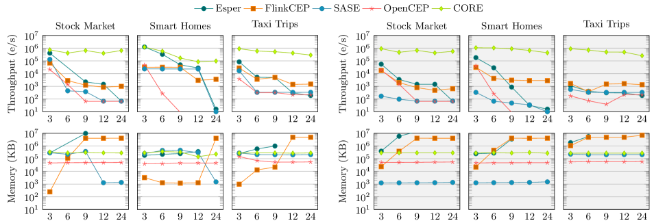
Figure 7. Throughput (higher is better) and memory consumption (lower is better) as a function of sequence length $n$, on queries with output (left) and queries without outputs (right, in gray).

In the following analysis, when the processing of an input event triggers one or more complex events to be recognized, we will refer to this triggering input event as a pattern occurrence. Each pattern occurrence may generate multiple complex event outputs. In our experiments, when a pattern occurrence is found, we only enumerate the first thousand corresponding complex events outputs. An exception is FlinkCEP where, for implementation reasons, we only generate the first such output. Note that this favors FlinkCEP since it needs to produce less output. For OpenCEP we use the so-called ANY evaluation strategy, which is the only one that allows enumerating all matches. Unfortunately, it does not produce the same outputs as CORE, SASE, and FlinkCEP. Despite this, the number of results produced by OpenCEP is similar to other systems, making the comparison reasonable.

Figure 7 (left), plots the measured throughput and memory consumption (in log scale) as a function of the sequence length $n$. CORE’s throughput is in the range of $[10^{5},10^{6}]$ e/s. This throughput fluctuates due to variations in the number of complex events found, which must all be reported before an event can be declared fully processed. For example, for the smart homes dataset, queries $P_{9}$ and $P_{12}$ are very output intensive (i.e., around 1 million pattern occurrences in total), and the fluctuations are most noticeable for this dataset. Instead, the stocks and taxi trips datasets have less pattern occurrences (i.e., around a few thousand) and we can see that CORE’s throughput is more stable. Note in particular that CORE’s throughput is only linearly affected by $n$ in these cases.

We next compare to the other systems. For $n=3$, the throughput of most baselines is one order of magnitude (OOM) lower than CORE, except for Esper which has comparable throughput on stock and smart homes. However, as $n$ grows, the throughput of all systems except CORE degrades exponentially. For the smart homes dataset, the throughput of FlinkCEP is more stable, although up to 2 OOM lower than CORE. Recall, however, that FlinkCEP produces only a single complex event per pattern occurrence, while all other systems enumerate up to one thousand complex events per occurrence. In contrast to the baselines, CORE’s throughput is stable, only affected by the high number of complex events found, and degrades only linearly in $n$ on stocks and taxis. As a consequence, on these datasets, CORE’s throughput is 1 to 5 OOM higher than the baselines for large values of $n$.

The memory used by CORE is high ($\sim$300MB) but stable in $n$. By contrast, the memory consumption of Esper and FlinkCEP can grow exponentially in $n$. OpenCEP and SASE are special cases whose memory consumption is stable and comparable to CORE.

Sequence queries without output. In practice, we may expect CER systems to look for unusual patterns in the sense that the number of complex events found is small. Our next experiment captures this setting. For each query $P_{n}$ we create a variant $P_{n}^{\prime}$ by adding, to the sequence pattern of $P_{n}$, an additional event that never occurs in the stream. These variant queries hence never produce outputs. Since systems do not know this, however, they must inherently look for partial matches that satisfy the original sequence query $P_{n}$. Because no time is spent enumerating complex events when processing $P_{n}^{\prime}$, this experiment can hence also be viewed as a way of measuring only the update performance of $P_{n}$. Note that, even though no complex events are found, systems may still materialize a large number of partial matches.

Figure 7 (right) plots the results (in log scale) on $P_{n}^{\prime}$ for $n=3$, $6$, $9$, $12$, $24$. We see that CORE’s throughput is comparable to the throughput on $P_{n}$ (Figure 7, left), except for the smart homes dataset, where the throughput has improved. Overall, CORE’s throughput is on the order of $10^{6}$ e/s, decreasing mostly linearly with $n$. By contrast, other systems have lower throughput, by 1 to 5 OOM, and this throughput decreases much more rapidly in $n$. This is most observable for Esper and OpenCEP, whose performance drops exponentially in $n$. For the taxi dataset, the throughput of all systems reduces to less $10^{4}$ e/s compared to the original $P_{n}$ setting, most probably because of a high number of partial matches that are maintained but never completed. CORE is not affected by the number of partial matches, which explains its stable performance.

Notice that CORE does not use lazy evaluation (Mei and Madden, 2009; Kolchinsky et al., 2015; Kolchinsky and Schuster, 2018) as some other systems do: it eagerly updates its internal data structure on each input event.A CER system that uses lazy evaluation could perform well when there is no output (i.e., for $P_{n}^{\prime}$) but badly when several pattern occurrences appear (i.e., for $P_{n}$). One can see CORE as the best of both worlds. It does work event after event, and results are ready for enumeration at each pattern occurrence.

Memory consumption of most systems remains high, with the memory usage of Esper and FlinkCEP increases exponentially with $n$. CORE’s memory consumption is stable, like the consumption of SASE and OpenCEP.

Varying the time-window size. We next measure the effect of varying the time window size on processing performance. We do so by fixing query $P^{\prime}_{3}$, and varying the window size from T to 4T where T is the original window size. We fix $P_{3}^{\prime}$ because this allows us to measure the effect of update processing only, and because performance on $P_{n}^{\prime}$ is highest for all systems when $n=3$.

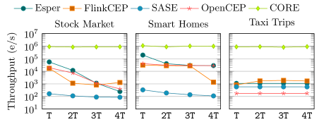
Figure 8. Throughput as a function of time-window size.

The results (log scale) are in Figure 8. We see that CORE outperforms other systems by at least one OOM for size T and by 2 to 4 OOM for 4T. Note that for stock market and smart homes dataset we are still using relatively small time windows of a few hundreds events; in practice windows may be significantly larger (e.g., taxi trips dataset). We also observe that the throughput of other systems may degrade exponentially as the size of the time window grows. Indeed, this is clear for Esper, FlinkCEP, and OpenCEP on stock market dataset, where the throughput is around $10^{5}$ e/s at T but less than $10^{3}$ e/s at 4T. In contrast, CORE consistently maintains its performance at $10^{6}$ e/s, and it is not affected by the window size, as the theoretical analysis predicted.

In Appendix H, we report similar experimental results even when all systems are allowed to use a selection strategy heuristic to aid in faster processing.

Other operators. For the last experiment, we consider a diverse workload of queries where other operators like disjunction, iteration, or partition-by are used. For these queries, we report only on the stock market dataset. Given space restrictions, we present the full CEQL definition of each query in the online appendix (sys, [n.d.]), and limit ourselves here to the the following simplified description.

$Q_{1}$  :=  SELL ; BUY ; BUY ; SELL

$Q_{2}$  :=   $Q_{1}$ + FILTER

$Q_{3}$  :=   $Q_{1}$ + PARTITION BY

$Q_{4}$  :=   SELL ; (BUY OR SELL) ; (BUY OR SELL) ; SELL

$Q_{5}$  :=   $Q_{4}$ + FILTER

$Q_{6}$  :=   $Q_{4}$ + PARTITION BY

$Q_{7}$  :=   SELL ; (BUY OR SELL)+ ; SELL

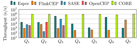
Figure 9. Throughput of evaluating queries $Q_{1}$ to $Q_{7}$, which include non-sequence operators, over stock market data.

SASE and OpenCEP do not support disjunction, and we hence omit $Q_{4}$–$Q_{7}$ for them. Queries $Q_{3}$ and $Q_{6}$ use the partition-by clause. Unfortunately, every system gave different outputs when we tried partition-by queries. Therefore, for $Q_{3}$ and $Q_{6}$ we cannot guarantee query equivalence for all systems. In all other cases, the results provided by each system are the same.

In Figure 9 we show the throughput (log-scale), grouped per query. The results confirm our observations from the previous experiments. In particular, CORE’s throughput is stable over all queries (i.e., $10^{6}$ e/s), in contrast to the baselines, which are not stable. In particular for every baseline system there is at least one query where CORE’ exhibits 2 OOM or more higher throughput.

$Q_{2}$ and $Q_{5}$ add filter clauses to $Q_{1}$ and $Q_{4}$ respectively. If we contrast system performance on $Q_{2}$ and $Q_{5}$ with that on $Q_{1}$ and $Q_{4}$, respectively, then we see that adding such filters reduces performance of some baselines, most notably SASE and Esper. CORE does not suffer from these problems due to its evaluation algorithm.

$Q_{3}$ and $Q_{6}$ add a partition-by clause to $Q_{1}$ and $Q_{4}$, respectively. If we contrast system performance on $Q_{3}$ and $Q_{6}$ with that on $Q_{1}$ and $Q_{4}$, respectively, then we see that partition-by aids the performance of systems like Esper and SASE but slightly decreases the throughput of CORE. This is because CORE  evaluate the partition-by clause by running several instances of the main algorithm, one for each partition, which slightly diminishes the throughput. Nevertheless, CORE still outperforms the baselines.

Limitations of CORE. As the previous experiments show, CORE outperforms other systems by several orders of magnitudes on different query and data workloads. We finish this section by a discussion of the limitations of CORE.

In particular, we see two limitations compared to other approaches. First, CORE’s asymptotically optimal performance comes from representing partial matches succinctly in a compact structure, and enumerating complex events from this structure whenever a pattern occurrence is found. The enumeration is with output-linear delay, meaning that the time spent to enumerate complex event $C$ is asymptotically $\mathcal{O}(|C|)$, i.e., linear in $C$. This asymptotic analysis hides a constant factor. While our experiments show that this constant is negligible in practice, enumeration from the data structure may take longer than directly fetching the complex event from an uncompressed representation, as most other systems do. This difference may be important in situations where a user wants to access outputs multiple times.

Second, CORE compiles CEQL queries into non-deterministic CEA, which need to be (on-the-fly) determinized before execution. In the worst case, this determinized CEA can be of size exponential in the size of the query. Since the time needed to process a new event tuple, while constant in data complexity, does depends on the CEA size (Section 4.3), this may also affect processing performance. While we did not observe this blowup on the queries in this section, CEQL queries with complicated nesting of iteration and disjunction can theoretically exhibit such behavior. Unfortunately, no baseline system (except CORE) currently allows such nesting, and we are therefore unable to experimentally compare CORE in such a setting.

6. Conclusions and future work

We introduced CORE, a CER system whose evaluation algorithm guarantees constant time per event, followed by output-linear delay enumeration. To the best of our knowledge, CORE is the first system that supports both guarantees. We showed through experiments that the evaluation algorithm provides stable performance for CORE, which is not affected by the size of the stream, query, or time window. This property means a throughput up to five orders of magnitudes higher than leading systems in the area.

CORE provides a novel query evaluation approach; however, there is space for several improvements. A natural problem is to extend CEQL to allow time windows or partition-by operators inside the WHERE clause, which will increase the expressive power of CEQL. We currently do not know how to extend the evaluation algorithm for such queries while maintaining the performance guarantees. Other relevant features to include in CORE are aggregation, integration of non-event data sources, or the algorithm’s parallelization, among others, which we leave as future work.

Appendix A Proofs of Section 2

A.1. Proof of Theorem 2

See 2

Proof.

This result follows almost directly from the proof for Theorem 6.2 in (Grez et al., 2021), which states that for every (unary) CEL formula $\varphi$ there is an equivalent CEA $\mathcal{A}$. However, there are certain subtleties that need to be addressed so that this result translates into ours. For completeness, we present here the construction of (Grez et al., 2021), modified to fit our setting with intervals. However, it is worth noting that the only three differences in the construction are in the cases $\varphi=R$, $\varphi=\psi_{1}\,;\,\psi_{2}$ and $\varphi=\psi+$, in order to handle the fact that now a run may start at an arbitrary position $i$ in the stream.

In (Grez et al., 2021), they use an extended model of CEA, which replaces the $\bullet,\circ$ marks in the transitions with subsets of variables. Formally, a valuation complex event automaton (VCEA) is a tuple $\mathcal{A}=(Q,\Delta,I,F)$, where $Q$ is the set of states, $I,F\subseteq Q$ are the set of initial and final states, respectivelly, and $\Delta$ is the transition relation $\Delta\subseteq Q\times\mathbf{P}\times 2^{\mathbf{X}}\times Q$. The definitions of run and accepting run remain the same as for CEA, i.e., a run is a sequence $\rho\ :=\ q_{i}\,\raisebox{-1.0pt}[10.0pt][0.0pt]{$\overset{P_{i}/L_{i}}{\underset{}{\raisebox{0.0pt}[3.0pt][0.0pt]{$\relbar\mspace{-8.0mu}\longrightarrow$}}}$}\,q_{i+1}\,\raisebox{-1.0pt}[10.0pt][0.0pt]{$\overset{P_{i+1}/L_{i+1}}{\underset{}{\raisebox{0.0pt}[3.0pt][0.0pt]{$\relbar\mspace{-8.0mu}\longrightarrow$}}}$}\,\ldots\,\raisebox{-1.0pt}[10.0pt][0.0pt]{$\overset{P_{j}/L_{j}}{\underset{}{\raisebox{0.0pt}[3.0pt][0.0pt]{$\relbar\mspace{-8.0mu}\longrightarrow$}}}$}\,q_{j+1}$ such that $q_{i}\in I$ and for every $k\in[i,j]$ it holds that $q_{k}\raisebox{-1.0pt}[10.0pt][0.0pt]{$\overset{P_{k}/L_{k}}{\underset{}{\raisebox{0.0pt}[3.0pt][0.0pt]{$\relbar\mspace{-8.0mu}\longrightarrow$}}}$}q_{k+1}\in\Delta$ and $t_{k}\models P_{k}$; and $\rho$ is accepting if $q_{j+1}\in F$. Now $\rho$ defines a valuation $V_{\rho}\ :=\ ([i,j],\mu)$, where $\mu(X)=\{k\mid X\in L_{k}\}$, and we define the valuation semantics of $\mathcal{A}$ over a stream $S$ as ${\llceil{\mathcal{A}}\rrfloor}(S):=\{V_{\rho}\mid\text{$\rho$ is an accepting run of $\mathcal{A}$ over $S$}\}.$ Now, we say that a CEL formula $\varphi$ is equivalent to a VCEA if ${\llceil{\varphi}\rrfloor}(S)={\llceil{\mathcal{A}}\rrfloor}(S)$ for every stream $S$.

Consider any CEL formula $\varphi$. We can construct a VCEA $\mathcal{A}_{\varphi}$ that is equivalent to $\varphi$ by induction on $\varphi$, as follows.

Figure 10. A VCEA for the atomic formula $R$. Here, $P_{R}=\{t\mid t(\operatorname{type})=R\}$.

• If $\varphi=R$, then $\mathcal{A}_{\varphi}$ is defined as depicted in Figure 10, i.e. $\mathcal{A}_{\varphi}=(\{q_{1},q_{2}\},\{(q_{1},P_{R},\{R\},q_{2})\},\{q_{1}\},\{q_{2}\})$, where $P_{R}$ is the predicate containing all tuples with type $R$, namely, $P_{R}:=\{t\mid t(\operatorname{type})=R\}$.

• If $\varphi=\psi~{}\operatorname{AS}~{}X$, then $\mathcal{A}_{\varphi}=(Q_{\psi},\Delta_{\varphi},I_{\psi},F_{\psi})$ where $\Delta_{\varphi}$ is the result of adding variable $X$ to all marking transitions of $\Delta_{\psi}$, i.e., $\Delta_{\varphi}=\{(p,P,L,q)\in\Delta_{\psi}\mid L=\emptyset\}\cup\{(p,P,L,q)\mid\exists L^{\prime}\neq\emptyset\text{ such that }(p,P,L^{\prime},q)\in\Delta_{\psi}\land L=L^{\prime}\cup\{X\}\}$.

• If $\varphi=\psi~{}\mathtt{FILTER}~{}X\texttt{[}P\texttt{]}$ for some variable $X$ and predicate $P$, then $\mathcal{A}_{\varphi}=(Q_{\psi},\Delta_{\varphi},I_{\psi},F_{\psi})$ where $\Delta_{\varphi}$ is defined as $\{(p,P^{\prime},L,q)\in\Delta_{\psi}\mid X\notin L\}\cup\{(p,P\wedge P^{\prime},L,q)\mid(p,P^{\prime},L,q)\in\Delta_{\psi}\land X\in L\}$.

• If $\varphi=\psi_{1}~{}\mathtt{OR}~{}\psi_{2}$, then $\mathcal{A}_{\varphi}$ is the automata union between $\mathcal{A}_{\psi_{1}}$ and $\mathcal{A}_{\psi_{2}}$: $\mathcal{A}_{\varphi}=(Q_{\psi_{1}}\cup Q_{\psi_{2}},\Delta_{\psi_{1}}\cup\Delta_{\psi_{2}},I_{\psi_{1}}\cup I_{\psi_{2}},F_{\psi_{1}}\cup F_{\psi_{2}})$. Here, we assume w.l.o.g. that $\mathcal{A}_{\psi_{1}}$ and $\mathcal{A}_{\psi_{2}}$ have disjoint sets of states.

• If $\varphi=\psi_{1}\,;\,\psi_{2}$, then $\mathcal{A}_{\varphi}=(Q_{\psi_{1}}\cup Q_{\psi_{2}},\Delta_{\varphi},I_{\psi_{1}},F_{\psi_{2}})$ where $\Delta_{\varphi}=\Delta_{\psi_{1}}\cup\Delta_{\psi_{2}}\cup\{(p,\mathtt{TRUE},\emptyset,p)\mid p\in I_{\psi_{2}}\}\cup\{(p,P,L,q)\mid q\in I_{\psi_{2}}\land\exists q^{\prime}\in F_{\psi_{1}}.(p,P,L,q^{\prime})\in\Delta_{\psi_{1}}\}$. Here, we assume w.l.o.g. that $\mathcal{A}_{\psi_{1}}$ and $\mathcal{A}_{\psi_{2}}$ have disjoint sets of states.

• If $\varphi=\psi+$, then $\mathcal{A}_{\varphi}=(Q_{\psi}\cup\{q\},\Delta_{\varphi},I_{\psi},F_{\psi})$ where $q$ is a fresh state, $\Delta_{\varphi}=\Delta_{\psi}\cup\{(p,P,L,q)\mid\exists q^{\prime}\in F_{\psi}.(p,P,L,q^{\prime})\in\Delta_{\psi}\}\cup\{(q,P,L,p)\mid\exists q^{\prime}\in I_{\psi}.(q^{\prime},P,L,p)\in\Delta_{\psi}\}$.

• If $\varphi=\pi_{L}(\psi)$ for some $L\subseteq\mathbf{L}$, then $\mathcal{A}_{\varphi}=(Q_{\psi},\Delta_{\varphi},I_{\psi},F_{\psi})$ where $\Delta_{\varphi}$ is the result of intersecting the labels of each transition in $\Delta_{\psi}$ with $L$. Formally, that is $\Delta_{\varphi}=\{(p,P,L\cap L^{\prime},q)\mid(p,P,L^{\prime},q)\in\Delta_{\psi}\}$.

Note that in the VCEA model we replaced $q_{0}$ with a subset of states $I$. This is not a problem, since one can modify the final automaton to have only one initial state by adding a fresh state $q_{0}$ and replicating every transition coming from an initial state to go from $q_{0}$, i.e., adding transitions $\{(q_{0},P,L,q)\mid\exists p\in I.(p,P,L,q)\in\Delta\}$. This also assures that $q_{0}$ has no incoming transitions. From now on, we assume that $\mathcal{A}_{\varphi}$ has only one initial state $q_{\varphi}$.

Now that we have a VCEA $\mathcal{A}_{\varphi}=(Q_{\varphi},\Delta_{\varphi},q_{\varphi},F_{\varphi})$ that is equivalent to $\varphi$, we can construct a CEA $\mathcal{A}$ by changing the sets in the transitions with $\bullet,\circ$ marks. More precisely, we define $\mathcal{A}=(Q_{\varphi},\Delta,q_{\varphi},F_{\varphi})$ where $\Delta=\{(p,P,\bullet,q)\mid(p,P,L,q)\in\Delta_{\varphi}\land L\neq\emptyset\}\cup\{(p,P,\circ,q)\mid(p,P,L,q)\in\Delta_{\varphi}\land L=\emptyset\}$. One can verify that this CEA satisfies the theorem. ∎

Appendix B Proofs of Section 4

B.1. Proof of Theorem 3

See 3

Proof.

Consider a $k$-bounded and time-ordered tECD $\mathcal{E}$, a duplicate-free node n of $\mathcal{E}$, a time-window bound $\epsilon$ and a position $j$. We provide Algorithm 2 and show that: (1) it enumerates the set ${\llbracket{}{\texttt{n}}\rrbracket}_{\mathcal{E}}^{\epsilon}(j)$, and (2) it does so with output-linear delay. To simplify presentation in what follows, we denote the sets of bottom, output and union nodes by $N_{B}$, $N_{O}$ and $N_{U}$, respectively.

Algorithm 2 Enumeration of ${\llbracket{}{\texttt{n}}\rrbracket}_{\mathcal{E}}^{\epsilon}(j)$.

1:procedure Enumerate($\mathcal{E},\texttt{n},\epsilon,j$)

2:     $\texttt{st}\leftarrow\textsf{new-stack}()$

3:     $\tau\leftarrow j-\epsilon$

4:     if $\text{max}(\texttt{n})\geq\tau$ then

5:         $\textsf{push}(\texttt{st},(\texttt{n},\emptyset))$      

6:     while $(\texttt{n}^{\prime},P)\leftarrow\textsf{pop}(\texttt{st})$ do

7:         while true do

8:              if $\texttt{n}^{\prime}\in N_{B}$ then

9:                  $\texttt{output}([\textsf{pos}(\texttt{n}^{\prime}),j],P)$

10:                  break

11:              else if $\texttt{n}^{\prime}\in N_{O}$ then

12:                  $P\leftarrow P\cup\{\textsf{pos}(\texttt{n}^{\prime})\}$

13:                  $\texttt{n}^{\prime}\leftarrow\textsf{next}(\texttt{n}^{\prime})$

14:              else if $\texttt{n}^{\prime}\in N_{U}$ then

15:                  if $\text{max}(\textsf{right}(\texttt{n}^{\prime}))\geq\tau$ then

16:                       $\textsf{push}(\texttt{st},(\textsf{right}(\texttt{n}^{\prime}),P))$                   

17:                  $\texttt{n}^{\prime}\leftarrow\textsf{left}(\texttt{n}^{\prime})$                             

Algorithm 2 uses a stack st with the typical stack operations: $\textsf{new-stack}()$ to initialize an empty stack, $\textsf{push}(\texttt{st},e)$ to add an element $e$ at the beginning of st, and $\textsf{pop}(\texttt{st})$ to get the first element in st. Moreover, when st is empty, $e\leftarrow\textsf{pop}(\texttt{st})$ is interpreted as false. We assume that each of the previous operations can be performed in constant time.

Recall that $\mathcal{E}$ encodes a directed acyclic graph (DAG) $G_{\mathcal{E}}=(N,E)$ where $N$ are the vertices, and edges goes from any union node u to $\textsf{left}(\texttt{u})$ and $\textsf{right}(\texttt{u})$, and from any output node o to $\textsf{next}(\texttt{o})$. For every node $\texttt{n}^{\prime}\in N$ reachable from n and a threshold $\tau\geq 0$, let $\operatorname{paths}_{\geq\tau}(\texttt{n}^{\prime})$ be all paths of $G_{\mathcal{E}}$ that start at $\texttt{n}^{\prime}$ and end at some bottom node b with $\textsf{pos}(\texttt{b})\geq\tau$. It is clear that there exists a bijection between ${\llbracket{}{\texttt{n}^{\prime}}\rrbracket}_{\mathcal{E}}^{\epsilon}(j)$ and $\operatorname{paths}_{\geq j-\epsilon}(\texttt{n}^{\prime})$, namely, for every complex event within a time window of size $\epsilon$ there exists exactly one path that reaches a bottom node b with $\textsf{pos}(\texttt{b})\geq j-\epsilon$ (this is true because, since n is duplicate-free, so must be $\texttt{n}^{\prime}$). Then, Algorithm 2 receives as input a tECD $\mathcal{E}$, a node n, a time-window bound $\epsilon$ and a position$j$, and traverses $G_{\mathcal{E}}$ in a DFS manner and following the left-to-right order, i.e., for every union node u, the paths of $\textsf{left}(\texttt{u})$ are traversed before the ones of $\textsf{right}(\texttt{u})$. Each iteration of the while of line 6 traverses a new path starting from the point it branches from the previous path. For this, the stack st is used to store the node and partial complex event of that branching point. Then, the while of line 7 traverses through the nodes of the next path, following the left direction whenever a union node is reached and adding the right node to the stack whenever needed. Moreover, by checking for every node $\texttt{n}^{\prime}$ its value $\text{max}(\texttt{n}^{\prime})$ before adding it to the stack, it makes sure of only going through paths in $\operatorname{paths}_{\geq j-\epsilon}(\texttt{n}^{\prime})$.

A simpler recursive algorithm could compute the same results. However, if done in a naive way, the output-linear delay might not be assured because when going back from a path to compute the next one, the number of backtracking steps might be as long as the longest path of $G_{\mathcal{E}}$. To avoid this, Algorithm 2 uses the stack st which allows it to jump immediately to the node that continues the next path. Here we assume that storing $P$ in the stack takes constant time. We can realize this assumption by representing $P$ as a linked list of positions, where the list is ordered by the last element added and there is a link to the previous element. Then for storing $P$ we can save in st a pointer to the last element added.

We first prove that Algorithm 2 enumerates the set ${\llbracket{}{\texttt{n}}\rrbracket}_{\mathcal{E}}^{\epsilon}(j)$, provided that $\mathcal{E}$ is time-ordered and n a duplicate-free node.

Lemma 0.

Let $\mathcal{E}$ be a time-ordered tECD, n a duplicate-free node of $\mathcal{E}$ and $\epsilon$ a time-window. Then, Algorithm 2 enumerates ${\llbracket{}{\texttt{n}}\rrbracket}_{\mathcal{E}}^{\epsilon}(j)$ without duplicates.

Proof.

For the rest of this proof fix a tECD $\mathcal{E}$ and a threshold $\tau=j-\epsilon$. For every node m of tECD, let $l_{\texttt{m}}$ be the longest path from m to a bottom node. We say a pair $(\texttt{m},R)$ of a node and a set of positions is visited if at some iteration of the while in line 7, variables $\texttt{n}^{\prime}$ and $P$ take the values m and $R$, respectively. Moreover, we say $(\texttt{m},R)$ is left when the pair $(\texttt{m}^{\prime},R^{\prime})$ is popped from the stack, where $(\texttt{m}^{\prime},R^{\prime})$ is the top of the stack when $(\texttt{m},R)$ was visited (or when the algorithm ends, if the stack was empty). The enumeration period of $(\texttt{m},R)$ is the period between it being visited and it being left. Intuitively, in the enumeration period of $(\texttt{m},R)$ is when the subtree rooted at m is enumerated.

Now, we prove that for every visited pair $(\texttt{m},R)$, the set $[\texttt{m}](R,j)=\{([i,j],D\cup R)\mid(i,D)\in{\llbracket{}{\texttt{m}}\rrbracket}_{\mathcal{E}}\land i\geq\tau\}$ is output in its enumeration period without duplicates. If this is the case, then it is clear that Lemma 1 holds, since, upon calling $\textsc{Enumerate}(\mathcal{E},\texttt{n},\epsilon,j)$ the pair $(\texttt{n},\emptyset)$ is the first one visited, and the enumerated set corresponds to $[\texttt{n}](\emptyset,j)=\{([i,j],D)\mid(i,D)\in{\llbracket{}{\texttt{n}}\rrbracket}_{\mathcal{E}}\land i\geq\tau\}={\llbracket{}{\texttt{n}}\rrbracket}_{\mathcal{E}}^{\epsilon}(j)$.

We prove the above by strong induction over $l_{\texttt{m}}$. The base case is when $l_{\texttt{m}}=0$, which means that m must be itself a bottom node. In that case, it enters in the if of line 8, outputs the corresponding complex event $([\textsf{pos}(\texttt{m}),j],R)$, clearly without duplicates. Note that ${\llbracket{}{\texttt{m}}\rrbracket}_{\mathcal{E}}=\{\textsf{pos}(\texttt{m}),\emptyset\}$ and that $\text{max}(\texttt{m})\geq\tau$, so $\textsf{pos}(\texttt{m})\geq\tau$ and the statement holds.

Now for the inductive step, consider $l_{\texttt{m}}>0$, which means that m is either an output node or a union node. In the former case, after entering the if of line 11, $P$ and $\texttt{n}^{\prime}$ are updated to $R\cup\{\textsf{pos}(\texttt{m})\}$ and $\textsf{next}(\texttt{m})$, respectively, and the new iteration of the while begins with those values. Then, since $l_{\textsf{next}(\texttt{m})}=l_{\texttt{m}}-1$, by induction hypothesis the set $[\textsf{next}(\texttt{m})](R\cup\{\textsf{pos}(\texttt{m})\},j)$ is enumerated, but by definition ${\llbracket{}{\texttt{m}}\rrbracket}_{\mathcal{E}}=\{(i,D^{\prime}\cup\{\textsf{pos}(\texttt{m})\})\mid(i,D^{\prime})\in{\llbracket{}{\textsf{next}(\texttt{m})}\rrbracket}_{\mathcal{E}}\}$, so

$$[\textsf{next}(\texttt{m})](R\cup\{\textsf{pos}(\texttt{m})\},j)\;=\;\{([i,j],D^{\prime}\cup R\cup\{\textsf{pos}(\texttt{m})\})\mid(i,D^{\prime})\in{\llbracket{}{\textsf{next}(\texttt{m})}\rrbracket}_{\mathcal{E}}\land i\geq\tau\}\;=\;[\texttt{m}](R,j).$$

Therefore, the enumerated set corresponds to $[\texttt{m}](R,j)$. Also, by induction hypothesis this set is enumerated without duplicates and the statement holds.

If m is a union node, the if of line 14 is entered, which first pushes the pair $(\textsf{right}(\texttt{m}),R)$ if $\text{max}(\textsf{right}(\texttt{m}))\geq\tau$ and then updates $\texttt{n}^{\prime}$ to $\textsf{left}(\texttt{m})$ before continuing with the next iteration. Since $l_{\textsf{left}(\texttt{m})}$ and $l_{\textsf{right}(\texttt{m})}$ are not greater than $l_{\texttt{m}}-1$, by induction hypothesis, both sets $[\textsf{left}(\texttt{m})](R,j)$, $[\textsf{right}(\texttt{m})](R,j)$ are enumerated without duplicates (note that after enumerating $[\textsf{left}(\texttt{m})](R,j)$, the pair $(\textsf{right}(\texttt{m}),R)$ is popped). Because ${\llbracket{}{\texttt{u}}\rrbracket}_{\mathcal{E}}={\llbracket{}{\textsf{left}(\texttt{u})}\rrbracket}_{\mathcal{E}}\uplus{\llbracket{}{\textsf{right}(\texttt{u})}\rrbracket}_{\mathcal{E}}$, then this enumerated set corresponds to $[\textsf{left}(\texttt{m})](R,j)\cup[\textsf{right}(\texttt{m})](R,j)=[\texttt{m}](R,j)$. Also, since $\texttt{n}^{\prime}$ is duplicate-free, this set is enumerated without duplicates and the statement holds.

It has been proved that the set ${\llbracket{}{\texttt{n}}\rrbracket}_{\mathcal{E}}^{\epsilon}(j)$ is enumerated without duplicates. ∎

Now that the correctness of the algorithm has been proved, we proceed to show that the enumeration is performed with output-linear delay.

Lemma 0.

Fix $k$. Let $\mathcal{E}$ be a $k$-bounded and time-ordered tECD, n a node of $\mathcal{E}$ and $\epsilon$ a time-window. Then, Algorithm 2 enumerates ${\llbracket{}{\texttt{n}}\rrbracket}_{\mathcal{E}}^{\epsilon}(j)$ with output-linear delay.

Proof.

Fix $\mathcal{E}$ and $\tau$. We showed that Algorithm 2 traverses all paths of $\operatorname{paths}_{\geq\tau}(\texttt{n})$. Moreover, the order in which paths are traversed is completely determined by the order of the union nodes: for each union node u, the paths to its left are traversed first, and then the ones to its right. Formally, for every node $\texttt{n}^{\prime}$ define the leftmost path from $\texttt{n}^{\prime}$ as $\operatorname{\pi_{\vbox{\hbox{\scalebox{0.5}{$\swarrow$}}}}}(\texttt{n}^{\prime}):=\texttt{n}_{0}\rightarrow\texttt{n}_{1}\rightarrow\ldots\rightarrow\texttt{n}_{l}$ such that $\texttt{n}_{0}=\texttt{n}^{\prime}$ and, for every $i\leq l$:

• if $\texttt{n}_{i}\in N_{B}$, then $i=l$,

• if $\texttt{n}_{i}\in N_{O}$, then $\texttt{n}_{i+1}=\textsf{next}(\texttt{n}_{i})$, and

• if $\texttt{n}_{i}\in N_{U}$, then $\texttt{n}_{i+1}=\textsf{left}(\texttt{n}_{i})$.

Consider a path $\pi:=\texttt{n}_{0}\rightarrow\texttt{n}_{1}\rightarrow\ldots\rightarrow\texttt{n}_{l}$, and let $j\leq l$ be the last position such that $\texttt{n}_{j}$ is a union node, $\texttt{n}_{j+1}=\textsf{left}(\texttt{n}_{j})$ and $\text{max}(\textsf{right}(\texttt{n}_{j}))\geq\tau$. Then, let $\pi^{u}$ be the path $\pi$ up to position $j$, i.e., that stops at such union node.

Let $P=\{\pi_{1},\pi_{2},\ldots,\pi_{m}\}$ be the set of paths enumerated by Algorithm 2 in that order. Then, by analysing Algorithm 2, one can see that $\pi_{1}=\operatorname{\pi_{\vbox{\hbox{\scalebox{0.5}{$\swarrow$}}}}}(\texttt{n})$ and, for every $i\leq m$, $\pi_{i}=\pi_{i-1}^{u}\cdot\operatorname{\pi_{\vbox{\hbox{\scalebox{0.5}{$\swarrow$}}}}}(\textsf{right}(\texttt{u}))$, where u is the last node of $\pi_{i-1}^{u}$. In other words, it performs a greedy DFS from left to right: the first path to enumerate is $\pi_{1}=\operatorname{\pi_{\vbox{\hbox{\scalebox{0.5}{$\swarrow$}}}}}(\texttt{n})$, then each $\pi_{i}$ is the path of $\operatorname{paths}_{\geq\tau}(\texttt{n})$ that branches from $\pi_{i-1}$ to the right at the deepest level (u) and from there follows the leftmost path. Moreover, to jump from $\pi_{i-1}$ to $\pi_{i}$, the node popped by the stack is exactly u, that is, the last node of $\pi_{i-1}^{u}$.

To show that the enumeration is done with output-linear delay, we study how long it takes between enumerating the complex events of $\pi_{i-1}$ and $\pi_{i}$. Consider that $\pi_{i-1}$ was just traversed and its complex event was output by line 9. Then, the break of line 10 is executed, breaking the while of line 7. Afterwards, either the stack is empty and the algorithm ends, or a pair $(\texttt{m},R)$ is popped from the stack, where m corresponds to the last node of $\pi_{i-1}^{u}$. From that point, it is straightforward to see that the number of iterations of the while of line 7 (each taking constant time) is equal to the number of nodes $l$ in $\operatorname{\pi_{\vbox{\hbox{\scalebox{0.5}{$\swarrow$}}}}}(\texttt{m})$, so those nodes are traversed and the complex event of the path $\pi_{i}$ is output. But, because $\mathcal{E}$ is $k$-bounded, then $l\leq k\cdot|O|$, where $O$ is the complex event of $\pi_{i}$. Finally, the time taken is bounded by the size of the output, and the enumeration is performed with output-linear delay. ∎

By Lemmas 1 and  2, Theorem 3 immediately holds. ∎

B.2. Proof of Theorem 4

See 4

Proof.

Fix a CEA $\mathcal{A}=(Q,\Delta,q_{0},F)$ and a stream $S=t_{0}t_{2}\ldots$. Given a run of $\mathcal{A}$ over $S$ of the form $\rho:=q_{i}\raisebox{-1.0pt}[10.0pt][0.0pt]{$\overset{P_{i}/m_{i}}{\underset{}{\raisebox{0.0pt}[3.0pt][0.0pt]{$\relbar\mspace{-8.0mu}\longrightarrow$}}}$}q_{i+1}\raisebox{-1.0pt}[10.0pt][0.0pt]{$\overset{P_{i+1}/m_{i+1}}{\underset{}{\raisebox{0.0pt}[3.0pt][0.0pt]{$\relbar\mspace{-8.0mu}\longrightarrow$}}}$}\ldots\raisebox{-1.0pt}[10.0pt][0.0pt]{$\overset{P_{j}/m_{j}}{\underset{}{\raisebox{0.0pt}[3.0pt][0.0pt]{$\relbar\mspace{-8.0mu}\longrightarrow$}}}$}q_{j+1}$, let $o(\rho)=(i,D)$ where $D=\{k\mid i\leq k\leq j\land m_{k}=\bullet\}$ be the open complex event associated to $\rho$. For any position $j$ and a state $q\in Q$, let $R_{j}^{q}$ be the set of runs that reach $q$ after reading position $j$ of the stream, that is, $R_{j}^{q}=\{\rho\mid\exists i.\,\text{$\rho$ is a run of $\mathcal{A}$ over $S$ from positions $i$ to $j$}\}$. Further, let $CE_{j}^{q}=\{o(\rho)\mid\rho\in R_{j}^{q}\}$ be the set of corresponding open complex events.

For a union-list $\texttt{ul}=\texttt{n}_{0},\texttt{n}_{1},\ldots,\texttt{n}_{k}$, of a tECD $\mathcal{E}$ define its set of open complex events as expected: $o(\texttt{ul})={\llbracket{}{\texttt{n}_{0}}\rrbracket}_{\mathcal{E}}\cup\ldots\cup{\llbracket{}{\texttt{n}_{k}}\rrbracket}_{\mathcal{E}}$. Then, for a position $j$ and a state $q\in Q$ let $ACE_{j}^{q}=o(\operatorname{T}[q])$ be the set of open complex events stored by $\operatorname{T}[q]$ after reading position $j$ of the stream, i.e., after the $(j+1)$-th iteration of the while of line 4 of Algorithm 1.

Note that ${\llbracket{}{\mathcal{A}}\rrbracket}^{\epsilon}_{j}(S)=\{([i,j],D)\mid(i,D)\in\bigcup_{q\in F}CE_{j}^{q}\land j-i\leq\epsilon\}$. One can see that in Algorithm 1, if after the $j$-th iteration the underlying tECS $\mathcal{E}$ is time-ordered and $k$-bounded for some constant $k$ and all nodes of $\mathcal{E}$ are duplicate-free, then by Theorem 3 procedure Output enumerates the set $\{([i,j],D)\mid(i,D)\in\bigcup_{q\in F}ACE_{j}^{q}\land j-i\leq\epsilon\}$ with output-linear delay. Therefore, if we prove that, for every $j$ and $q$, (1) $CE_{j}^{q}=ACE_{j}^{q}$, (2) $\mathcal{E}$ is time-ordered and $k$-bounded and (3) all nodes in $\mathcal{E}$ are duplicate-free, then the theorem holds.

Before we start proving (1)-(3), let us first analyse procedure ExecTrans. At the beginning of iteration $j$, every $ACE^{q}_{j}$ starts empty. Then, every time $\textsc{ExecTrans}(p,\texttt{ul},t,j)$ is called, it takes all open complex events in $ACE^{p}_{j-1}$ and:

• for $q_{\circ}=\Delta(p,t,\circ)$, it makes $ACE^{q_{\circ}}_{j}\leftarrow ACE^{q_{\circ}}_{j}\cup ACE^{p}_{j-1}$; and

• for $q_{\bullet}=\Delta(p,t,\bullet)$, it makes $ACE^{q_{\bullet}}_{j}\leftarrow ACE^{q_{\bullet}}_{j}\cup(ACE^{p}_{j-1}\times\{j\})$, where $ACE^{p}_{j-1}\times\{j\}=\{(i,D\cup\{j\})\mid(i,D)\in ACE^{p}_{j-1}\}$.

The two cases in Add just handle whether $ACE^{q_{\bullet}}_{j}$ or $ACE^{q_{\circ}}_{j}$ are empty at the moment or not.

We will prove (1) by simple induction over $j$. For the base case, consider the state before the first iteration, namely $j=-1$ and $\operatorname{T}=\emptyset$. It is easy to see that $CE_{-1}^{q}=ACE_{-1}^{q}=\emptyset$, so the property holds. Now for the inductive case, consider that $CE_{j}^{q}=ACE_{j}^{q}$. First, a new list with only a bottom node is created and stored in ul and then $\textsc{ExecTrans}(q_{0},\texttt{ul},t,j)$ is called. This starts possibly two runs from the initial state $q_{0}$ with either a $\circ$ or $\bullet$-transition. Then, $\textsc{ExecTrans}(q_{0},\operatorname{T}[p],t,j)$ is called for every state that is active before reading position $j$, i.e., for every $p$ with $ACE_{j}^{p}\neq\emptyset$. Let us consider any $(i,D)\in ACE_{j+1}^{q}$. If it came from the first call to ExecTrans, then it means that $i=j$ and, either $D=\{j\}$ and there is a run (from $j+1$ to $j+1$) of the form $\rho=q_{0}\raisebox{-1.0pt}[10.0pt][0.0pt]{$\overset{P/\bullet}{\underset{}{\raisebox{0.0pt}[3.0pt][0.0pt]{$\relbar\mspace{-8.0mu}\longrightarrow$}}}$}q$, or $D=\emptyset$ and there is a run (from $j+1$ to $j+1$) $\rho=q_{0}\raisebox{-1.0pt}[10.0pt][0.0pt]{$\overset{P/\circ}{\underset{}{\raisebox{0.0pt}[3.0pt][0.0pt]{$\relbar\mspace{-8.0mu}\longrightarrow$}}}$}q$. Either way, the corresponding run assures that $(i,D)\in CE_{j+1}^{q}$. Now, if $(i,D)$ came from one of the subsequent calls to ExecTrans, it means that there was some $(i,D^{\prime})\in ACE_{j}^{p}$ such that either $D=D^{\prime}$ and $q=\Delta(p,t_{j},\circ)$, or $D=D^{\prime}\cup\{j\}$ and $q=\Delta(p,t_{j},\bullet)$. Call such transition $e$. By induction hypothesis, there is a run from $i$ to $j$ $\rho=q_{i}\raisebox{-1.0pt}[10.0pt][0.0pt]{$\overset{P_{i}/m_{i}}{\underset{}{\raisebox{0.0pt}[3.0pt][0.0pt]{$\relbar\mspace{-8.0mu}\longrightarrow$}}}$}q_{i+1}\raisebox{-1.0pt}[10.0pt][0.0pt]{$\overset{P_{i+1}/m_{i+1}}{\underset{}{\raisebox{0.0pt}[3.0pt][0.0pt]{$\relbar\mspace{-8.0mu}\longrightarrow$}}}$}\ldots\raisebox{-1.0pt}[10.0pt][0.0pt]{$\overset{P_{j}/m_{j}}{\underset{}{\raisebox{0.0pt}[3.0pt][0.0pt]{$\relbar\mspace{-8.0mu}\longrightarrow$}}}$}p$ with $o(\rho)=(i,D^{\prime})$. Therefore, there is a run $\rho^{\prime}$ that extends $\rho$ with $e$ such that $o(\rho^{\prime})=(i,D)$ and $\rho^{\prime}\in R^{q}_{j+1}$, therefore $(i,D)\in ACE^{q}_{j+1}$. Then, $CE^{q}_{j+1}\subseteq ACE^{q}_{j+1}$. We can use the same analysis to prove that $ACE^{q}_{j+1}\subseteq CE^{q}_{j+1}$, thus $CE^{q}_{j+1}=ACE^{q}_{j+1}$ and the induction holds.

Now, we focus on proving (2). It has already been shown that every operation over tECS $\mathcal{E}$ used by Algorithm 1 preserves the time-ordered and $k$-boundedness for $k=3$, provided that every time we call $\textsf{union}(\texttt{n}_{1},\texttt{n}_{2})$, both $\texttt{n}_{1}$ and $\texttt{n}_{2}$ are safe nodes. In particular, since we only manage unions using union-lists, we only need to check that every time $\textsf{new-ulist}(\texttt{n})$ or $\textsf{insert}(\texttt{ul},\texttt{n})$ are called, the input node n is a safe one. This is easily verifiably by looking at lines 7, 17 and 24 of Algorithm 1 (for 17 and 24, recall that $\textsf{merge}(\texttt{ul})$ returns a safe node). Note that $\textsf{merge}(\texttt{ul})$ does not have any requirement, since its correct behaviour is ensured by using the other operations correctly. Therefore, at any moment in the evaluation, the underlying tECS $\mathcal{E}$ is time-ordered and 3-bounded. Note that $\textsf{insert}(\texttt{ul},\texttt{n})$ has another precondition: that $\text{max}(\texttt{n}_{0})\geq\text{max}(\texttt{n})$, where $\texttt{n}_{0}$ is the first node of ul. Since this does not relate directly with the correctness of the output of Algorithm 1, but with an overall correct behaviour of the algorithm, this property is discussed in the next section, along with another property that is needed to ensure constant update-time.

Next, we prove (3). By taking a look at Algorithm 1, one can see that the only ways it could add to $\mathcal{E}$ nodes with duplicates are with methods merge and insert, particularly in lines 14, 24 and 32. Fix a position $j$. Let $\operatorname{All-N}$ be the set all nodes in the union-list of some state at position $j$, i.e., $\operatorname{All-N}=\{\texttt{n}\mid\exists q.\exists i.T[q]=\texttt{n}_{0},\ldots,\texttt{n}_{l}\land\texttt{n}_{i}=\texttt{n}\}$, where $T[q]$ is its value at iteration $j$. If, for every two $\texttt{n}_{1},\texttt{n}_{2}\in\operatorname{All-N}$ with $\texttt{n}_{1}\neq\texttt{n}_{2}$ it holds that ${\llbracket{}{\texttt{n}_{i}}\rrbracket}_{\mathcal{E}}\cap{\llbracket{}{\texttt{n}_{j}}\rrbracket}_{\mathcal{E}}=\emptyset$, then all cases are solved and the algorithm creates no nodes with duplicates. One can see that each ${\llbracket{}{\texttt{n}}\rrbracket}_{\mathcal{E}}$ actually stores the open complex events for a disjoint set of runs. Then, if there were some $\texttt{n}_{1},\texttt{n}_{2}\in\operatorname{All-N}$ with ${\llbracket{}{\texttt{n}_{1}}\rrbracket}_{\mathcal{E}}\cap{\llbracket{}{\texttt{n}_{2}}\rrbracket}_{\mathcal{E}}\neq\emptyset$, it would mean that there are two different runs defining the same output, thus contradicting the fact that $\mathcal{A}$ is I/O-deterministic. Therefore, all nodes must define disjoint sets and Algorithm 1 only adds duplicate-free nodes to $\mathcal{E}$.

Finally, because (1)-(3) hold, also does the theorem. ∎

B.3. Special invariants of union-lists in Algorithm 1

In this section we discuss in more detail two invariants maintained by Algorithm 1 which are needed for its correct behaviour. Specifically, we prove that:

1. every time a node n is added to some union-list $\texttt{ul}=\texttt{n}_{0},\ldots,\texttt{n}_{k}$, it is the case that $\text{max}(\texttt{n}_{0})\geq\text{max}(\texttt{n})$; and

2. at any moment, the length of every union-list $\operatorname{T}[q]$ is smaller than the number of states of the automaton $\mathcal{A}$.

The former assures that the first node $\texttt{n}_{0}$ always remains a non-union node, while the latter is needed so that operations merge and insert take constant time (when $\mathcal{A}$ is fixed).

First, we focus on (1). This comes directly from the order in which we update the union-lists. As notation, for a non-empty union-list $\texttt{ul}=\texttt{n}_{0},\ldots,\texttt{n}_{k}$, we write $\text{max}(\texttt{ul})=\text{max}(\texttt{n}_{0})$. Consider any iteration $j\geq 0$ and let $q_{1},\ldots,q_{l}$ be the order given by $\textsf{ordered-keys}(\operatorname{T})$. One can prove that this order actually preserves the following property: $\text{max}(\operatorname{T}[q_{i}])\geq\text{max}(\operatorname{T}[q_{i+1}])$ for every $i<l$. One can prove this by simple induction over $j$. As consequence, if $\textsc{ExecTrans}(q_{i},\operatorname{T}[q_{i}],t,j)$ is called and we need to add some node n at some union-list ul, it must be that ul was the result of some previous call $\textsc{ExecTrans}(q_{k},\operatorname{T}[q_{k}],t,j)$ with $k<i$, and so $\text{max}(\texttt{ul})\geq\text{max}(\operatorname{T}[q_{k}])\geq\text{max}(\texttt{n})$.

Now we prove (2). First, we show a property about the possible maximum-start values at any iteration of the algorithm. For $j\geq 0$, we define the set of maximum-starts at iteration $j$ as $M_{j}=\{\text{max}(\operatorname{T}[q])\mid q\in\textsf{keys}(\operatorname{T})\}$. The property we use is that the set $M_{j}$ is closely restricted by the set $M_{j-1}$ of the previous iteration. Specifically, one can see that $M_{j}$ must always be a subset of $M_{j-1}$, with the possibility of adding the maximum-start $j$ if a new run begins at that iteration, i.e., $M_{j}\subseteq(M_{j-1}\cup\{j\})$. This is because the maximum-start of every union-list $\operatorname{T}[q]$ at some iteration came either from extending the already existing runs of the previous iteration, therefore maintaining its maximum-start, or from starting a new run with maximum-start $j$.

Consider any union-list $\operatorname{T}[q]$ created at iteration $j$. From (1), we know that we will only add to $\operatorname{T}[q]$ nodes n with $\text{max}(\texttt{n})\leq\text{max}(\operatorname{T}[q])$. Moreover, it is always the case that $\text{max}(\texttt{n})\in M_{j}$. This is clear for iteration $j$, but it actually holds for the following ones. Indeed, $\operatorname{T}[q]$ could actually receive insertions in some future iteration, call it $k$. However, since $\text{max}(\operatorname{T}[q])$ does not change and the new maximum-start values in $M_{k}$ are higher than $j\geq\text{max}(\operatorname{T}[q])$, the actual maximum-start values that could be added to $\operatorname{T}[q]$ are still in $M_{j}\cap M_{k}\subseteq M_{j}$. Therefore, the size of $\operatorname{T}[q]$ is bounded by $|M_{j}|\leq|Q|$.

Appendix C Other baseline systems

We have surveyed the literature for other systems to compare against, but have chosen to limit our experiments to SASE (Wu et al., 2006), Esper (Esp, [n.d.]), FlinkCEP (Fli, [n.d.]), and OpenCEP (Ope, [n.d.]), for the following reasons.

First, we cannot compare against systems that, while published in the literature, do not publish an accompanying implementation (e.g., ZStream (Mei and Madden, 2009), NextCEP (Schultz-Møller et al., 2009), DistCED (Pietzuch et al., 2003), SAP ESP (Zhang et al., 2017)) or whose implementation was discontinued in the last decade (e.g., Cayuga (Demers et al., 2006)). Second, we cannot compare against proposals that do not offer a CER query language or whose implementation does not allow running the queries considered here (e.g. CET (Poppe et al., 2017a), GRETA (Poppe et al., 2017b)). We do not consider comparison against system whose optimization focus is on additional CER features (Zhao et al., 2021; Hirzel, 2012; Zhao et al., 2020), such as load shedding (Zhao et al., 2020) or interacting with external, non-stream data sources (Zhao et al., 2021), for which the comparison would not be fair. Finally, we do not compare against streaming SQL systems like Spark and Flink SQL whose SQL-based query languages do not natively support basic CER operators, like sequencing and iteration.

We have run experiments to compare against TESLA/TRex (Cugola and Margara, 2010, 2012a) and Siddhi (Suhothayan et al., 2011; Sid, [n.d.]). Unfortunately, their event recognition features differ from CORE’s; in particular, they do not have dedicated support for count-based time windows. As such, they are not optimized for the use cases that we aim to test here. When we expressed simple sequence queries with time windows by means of other features in their query languages (e.g., by using inequality predicates), performance was so limited (i.e., a throughput of less than ten events per second), that we decided not to further report the results of TESLA/TRex and Siddhi.

Appendix D Stock market dataset

Dataset. We reuse the stock market dataset from (sto, [n.d.]) also used in related work (Poppe et al., 2021; Poppe et al., 2019, 2017a, 2017b) to evaluate the effectiveness of CER processing strategies. This dataset contains approximately 225k transaction records of 10 stocks from NYSE in a single day, listing stock name, transaction ID, volume, price, time, and transaction type (SELL/BUY). We use the transaction type to divide the dataset into two streams: one stream of SELL events, and one steam of BUY events.

Queries. The workload of sequence queries with output over the stock market dataset are the following queries of length $3$, $6$, $9$, $12$ and $24$, respectively:

ΨΨS3 = SELECT * FROM S
ΨΨ     WHERE (SELL as T1; BUY as T2; BUY as T3)
ΨΨ     FILTER T1[name = ’INTC’] AND T2[name = ’RIMM’] AND T3[name = ’QQQ’]
ΨΨ     WITHIN 10000 [stock_time]
Ψ
ΨΨS6 = SELECT * FROM S
ΨΨ     WHERE (SELL as T1; BUY as T2; BUY as T3;
ΨΨ            SELL as T4; BUY as T5; BUY as T6)
ΨΨ     FILTER T1[name = ’INTC’] AND T2[name = ’RIMM’] AND T3[name = ’QQQ’] AND
ΨΨ            T4[name = ’IPIX’] AND T5[name = ’AMAT’] AND T6[name = ’CSCO’]
ΨΨ     WITHIN 10000 [stock_time]
ΨΨ
ΨΨS9 = SELECT * FROM S
ΨΨ     WHERE (SELL as T1; BUY as T2; BUY as T3;
ΨΨ            SELL as T4; BUY as T5; BUY as T6;
ΨΨ            SELL as T7; BUY as T8; BUY as T9)
ΨΨ     FILTER T1[name = ’INTC’] AND T2[name = ’RIMM’] AND T3[name = ’QQQ’] AND
ΨΨ            T4[name = ’IPIX’] AND T5[name = ’AMAT’] AND T6[name = ’CSCO’] AND
ΨΨ            T7[name = ’YHOO’] AND T8[name = ’DELL’] AND T9[name = ’ORCL’]
ΨΨ     WITHIN 10000 [stock_time]
ΨΨ
ΨΨS12 = SELECT * FROM S
ΨΨ      WHERE (SELL as T1; BUY as T2; BUY as T3;
ΨΨ             SELL as T4; BUY as T5; BUY as T6;
ΨΨ             SELL as T7; BUY as T8; BUY as T9;
ΨΨ             SELL as T10; BUY as T11; BUY as T12)
ΨΨ      FILTER T1[name = ’INTC’] AND T2[name = ’RIMM’] AND T3[name = ’QQQ’] AND
ΨΨ             T4[name = ’IPIX’] AND T5[name = ’AMAT’] AND T6[name = ’CSCO’] AND
ΨΨ             T7[name = ’YHOO’] AND T8[name = ’DELL’] AND T9[name = ’ORCL’] AND
ΨΨ             T10[name = ’MSFT’] AND T11[name = ’INTC’] AND T12[name = ’RIMM’]
ΨΨ      WITHIN 10000 [stock_time]
ΨΨ
ΨΨS24 = SELECT * FROM S
ΨΨ      WHERE (SELL as T1; BUY as T2; BUY as T3;
ΨΨ             SELL as T4; BUY as T5; BUY as T6;
ΨΨ             SELL as T7; BUY as T8; BUY as T9;
ΨΨ             SELL as T10; BUY as T11; BUY as T12;
ΨΨ             SELL as T13; BUY as T14; BUY as T15;
ΨΨ             SELL as T16; BUY as T17; BUY as T18;
ΨΨ             SELL as T19; BUY as T20; BUY as T21;
ΨΨ             SELL as T22; BUY as T23; BUY as T24)
ΨΨ      FILTER T1[name = ’INTC’] AND T2[name = ’RIMM’] AND T3[name = ’QQQ’] AND
ΨΨ             T4[name = ’IPIX’] AND T5[name = ’AMAT’] AND T6[name = ’CSCO’] AND
ΨΨ             T7[name = ’YHOO’] AND T8[name = ’DELL’] AND T9[name = ’ORCL’] AND
ΨΨ             T10[name = ’MSFT’] AND T11[name = ’INTC’] AND T12[name = ’RIMM’] AND
ΨΨ             T13[name = ’INTC’] AND T14[name = ’RIMM’] AND T15[name = ’QQQ’] AND
ΨΨ             T16[name = ’IPIX’] AND T17[name = ’AMAT’] AND T18[name = ’CSCO’] AND
ΨΨ             T19[name = ’YHOO’] AND T20[name = ’DELL’] AND T21[name = ’ORCL’] AND
ΨΨ             T22[name = ’MSFT’] AND T23[name = ’INTC’] AND T24[name = ’RIMM’]
ΨΨ      WITHIN 10000 [stock_time]
Ψ

For the workload of sequence queries without output, we extend each query of the previous workload with a “non-existing” event. Queries S3’, S6’, S9’, S12’, and S24’ are the aforementioned extension of S3, S6, S9, S12, and S24, respectively :

ΨS3’ = SELECT * FROM S
Ψ      WHERE (SELL as T1; BUY as T2; BUY as T3; BUY as NE)
Ψ      FILTER T1[name = ’INTC’] AND T2[name = ’RIMM’] AND T3[name = ’QQQ’] AND NE[name = ’NotExists’]
Ψ      WITHIN 10000 [stock_time]
Ψ
ΨS6’ = SELECT * FROM S
Ψ      WHERE (SELL as T1; BUY as T2; BUY as T3;
Ψ             SELL as T4; BUY as T5; BUY as T6; BUY AS NE)
Ψ      FILTER T1[name = ’INTC’] AND T2[name = ’RIMM’] AND T3[name = ’QQQ’] AND
Ψ             T4[name = ’IPIX’] AND T5[name = ’AMAT’] AND T6[name = ’CSCO’] AND NE[name = ’NotExists’]
Ψ      WITHIN 10000 [stock_time]
Ψ
ΨS9’ = SELECT * FROM S
Ψ      WHERE (SELL as T1; BUY as T2; BUY as T3;
Ψ             SELL as T4; BUY as T5; BUY as T6;
Ψ             SELL as T7; BUY as T8; BUY as T9; BUY AS NE)
Ψ      FILTER T1[name = ’INTC’] AND T2[name = ’RIMM’] AND T3[name = ’QQQ’] AND
Ψ             T4[name = ’IPIX’] AND T5[name = ’AMAT’] AND T6[name = ’CSCO’] AND
Ψ             T7[name = ’YHOO’] AND T8[name = ’DELL’] AND T9[name = ’ORCL’] AND NE[name = ’NotExists’]
Ψ      WITHIN 10000 [stock_time]
Ψ
ΨS12’ = SELECT * FROM S
Ψ       WHERE (SELL as T1; BUY as T2; BUY as T3;
Ψ              SELL as T4; BUY as T5; BUY as T6;
Ψ              SELL as T7; BUY as T8; BUY as T9;
Ψ              SELL as T10; BUY as T11; BUY as T12; BUY AS NE)
Ψ       FILTER T1[name = ’INTC’] AND T2[name = ’RIMM’] AND T3[name = ’QQQ’] AND
Ψ              T4[name = ’IPIX’] AND T5[name = ’AMAT’] AND T6[name = ’CSCO’] AND
Ψ              T7[name = ’YHOO’] AND T8[name = ’DELL’] AND T9[name = ’ORCL’] AND
Ψ              T10[name = ’MSFT’] AND T11[name = ’INTC’] AND T12[name = ’RIMM’] AND NE[name = ’NotExists’]
Ψ       WITHIN 10000 [stock_time]
Ψ
ΨS24’ = SELECT * FROM S
Ψ       WHERE (SELL as T1; BUY as T2; BUY as T3;
Ψ              SELL as T4; BUY as T5; BUY as T6;
Ψ              SELL as T7; BUY as T8; BUY as T9;
Ψ              SELL as T10; BUY as T11; BUY as T12;
Ψ              SELL as T13; BUY as T14; BUY as T15;
Ψ              SELL as T16; BUY as T17; BUY as T18;
Ψ              SELL as T19; BUY as T20; BUY as T21;
Ψ              SELL as T22; BUY as T23; BUY as T24; BUY AS NE)
Ψ       FILTER T1[name = ’INTC’] AND T2[name = ’RIMM’] AND T3[name = ’QQQ’] AND
Ψ              T4[name = ’IPIX’] AND T5[name = ’AMAT’] AND T6[name = ’CSCO’] AND
Ψ              T7[name = ’YHOO’] AND T8[name = ’DELL’] AND T9[name = ’ORCL’] AND
Ψ              T10[name = ’MSFT’] AND T11[name = ’INTC’] AND T12[name = ’RIMM’] AND
Ψ              T13[name = ’INTC’] AND T14[name = ’RIMM’] AND T15[name = ’QQQ’] AND
Ψ              T16[name = ’IPIX’] AND T17[name = ’AMAT’] AND T18[name = ’CSCO’] AND
Ψ              T19[name = ’YHOO’] AND T20[name = ’DELL’] AND T21[name = ’ORCL’] AND
Ψ              T22[name = ’MSFT’] AND T23[name = ’INTC’] AND T24[name = ’RIMM’] AND NE[name = ’NotExists’]
Ψ       WITHIN 10000 [stock_time]

For the workload of sequence queries of length 3 with increasing time windows and without output, we use query S3’ and modify the size of the time window by $20$, $30$, and $40$ seconds as follow:

ΨS3’ = SELECT * FROM S
Ψ      WHERE (SELL as T1; BUY as T2; BUY as T3; BUY as NE)
Ψ      FILTER T1[name = ’INTC’] AND T2[name = ’RIMM’] AND T3[name = ’QQQ’] AND NE[name = ’NotExists’]
Ψ      WITHIN 10000 [stock_time]
Ψ
ΨS3’x2 = SELECT * FROM S
Ψ        WHERE (SELL as T1; BUY as T2; BUY as T3; BUY as NE)
Ψ        FILTER T1[name = ’INTC’] AND T2[name = ’RIMM’] AND T3[name = ’QQQ’] AND NE[name = ’NotExists’]
Ψ        WITHIN 20000 [stock_time]
Ψ
ΨS3’x3 = SELECT * FROM S
Ψ        WHERE (SELL as T1; BUY as T2; BUY as T3; BUY as NE)
Ψ        FILTER T1[name = ’INTC’] AND T2[name = ’RIMM’] AND T3[name = ’QQQ’] AND NE[name = ’NotExists’]
Ψ        WITHIN 30000 [stock_time]
Ψ
ΨS3’x4 = SELECT * FROM S
Ψ        WHERE (SELL as T1; BUY as T2; BUY as T3; BUY as NE)
Ψ        FILTER T1[name = ’INTC’] AND T2[name = ’RIMM’] AND T3[name = ’QQQ’] AND NE[name = ’NotExists’]
Ψ        WITHIN 40000 [stock_time]

Finally, for the last workout of sequence queries with selection strategies, we consider queries S3’, S3’x2, S3’x3, and S3’x4 and use the selection strategy provided by each system.

Appendix E Smart homes dataset

Dataset. We reuse the smart homes dataset from the DEBS 2014 Grand Challenge (sma, [n.d.]), which contains events originating from smart plugs deployed in private households. Each smart plug acts as a proxy between the wall power outlet and the device connected to it, and is equipped with sensors to measure power load and power work at a resolution of one measurement per second. The full dataset consists of over 4055 million measurements for 2125 plugs distributed across 40 houses. We select the substream of events of a single house, with house id 28. This substream contains data from 85 plugs distributed over 17 households in the stream. We process the first million events, focusing on load measurements only. Each event consists of an event id, the timestamp, the measured load value, the plug id, and the household id.

Queries. All queries look for sequences of measurements in different household that are above the dataset average load of 76 Watts, in a time window of $10$ seconds (note that the plug timestamp is in seconds). The workload of sequence queries with output over the smart homes dataset are the following queries of length $3$, $6$, $9$, $12$ and $24$, respectively.

ΨΨH3 = SELECT * FROM S
ΨΨ     WHERE (LOAD as L1; LOAD as L2; LOAD as L3) as L
ΨΨ     FILTER L[value > 76] AND
ΨΨ            L1[household_id = 0] AND L2[household_id = 2] AND L3[household_id = 4]
ΨΨ     WITHIN 10 [plug_timestamp]
ΨΨ
ΨΨH6 = SELECT * FROM S
ΨΨ     WHERE (LOAD as L1; LOAD as L2; LOAD as L3;
ΨΨ            LOAD as L4; LOAD as L5; LOAD as L6) as L
ΨΨ     FILTER L[value > 76] AND
ΨΨ            L1[household_id = 0] AND L2[household_id = 2] AND L3[household_id = 4] AND
ΨΨ            L4[household_id = 6] AND L5[household_id = 9] AND L6[household_id = 10]
ΨΨ     WITHIN 10 [plug_timestamp]

ΨΨH9 = SELECT * FROM S
ΨΨ     WHERE (LOAD as L1; LOAD as L2; LOAD as L3;
ΨΨ            LOAD as L4; LOAD as L5; LOAD as L6;
ΨΨ            LOAD as L7; LOAD as L8; LOAD as L9) as L
ΨΨ     FILTER L[value > 76] AND
ΨΨ            L1[household_id = 0] AND L2[household_id = 2] AND L3[household_id = 4] AND
ΨΨ            L4[household_id = 6] AND L5[household_id = 9] AND L6[household_id = 10] AND
ΨΨ            L7[household_id = 12] AND L8[household_id = 14] AND L9[household_id = 15]
ΨΨ     WITHIN 10 [plug_timestamp]
ΨΨ
ΨΨH12 = SELECT * FROM S
ΨΨ      WHERE (LOAD as L1; LOAD as L2; LOAD as L3;
ΨΨ             LOAD as L4; LOAD as L5; LOAD as L6;
ΨΨ             LOAD as L7; LOAD as L8; LOAD as L9;
ΨΨ             LOAD as L10; LOAD as L11; LOAD as L12) as L
ΨΨ      FILTER L[value > 76] AND
ΨΨ             L1[household_id = 0] AND L2[household_id = 2] AND L3[household_id = 4] AND
ΨΨ             L4[household_id = 6] AND L5[household_id = 9] AND L6[household_id = 10] AND
ΨΨ             L7[household_id = 12] AND L8[household_id = 14] AND L9[household_id = 15] AND
ΨΨ             L10[household_id = 4] AND L11[household_id = 9] AND L12[household_id = 10]
ΨΨ      WITHIN 10 [plug_timestamp]
ΨΨ
ΨΨH24 = SELECT * FROM S
ΨΨ      WHERE (LOAD as L1; LOAD as L2; LOAD as L3;
ΨΨ             LOAD as L4; LOAD as L5; LOAD as L6;
ΨΨ             LOAD as L7; LOAD as L8; LOAD as L9;
ΨΨ             LOAD as L10; LOAD as L11; LOAD as L12;
ΨΨ             LOAD as L13; LOAD as L14; LOAD as L15;
ΨΨ             LOAD as L16; LOAD as L17; LOAD as L18;
ΨΨ             LOAD as L19; LOAD as L20; LOAD as L21;
ΨΨ             LOAD as L22; LOAD as L23; LOAD as L24) as L
ΨΨ      FILTER L[value > 76] AND
ΨΨ             L1[household_id = 0] AND L2[household_id = 2] AND L3[household_id = 4] AND
ΨΨ             L4[household_id = 6] AND L5[household_id = 9] AND L6[household_id = 10] AND
ΨΨ             L7[household_id = 12] AND L8[household_id = 14] AND L9[household_id = 15] AND
ΨΨ             L10[household_id = 4] AND L11[household_id = 9] AND L12[household_id = 10] AND
ΨΨ             L13[household_id = 0] AND L14[household_id = 2] AND L15[household_id = 4] AND
ΨΨ             L16[household_id = 6] AND L17[household_id = 9] AND L18[household_id = 10] AND
ΨΨ             L19[household_id = 12] AND L20[household_id = 14] AND L21[household_id = 15] AND
ΨΨ             L22[household_id = 4] AND L23[household_id = 9] AND L24[household_id = 10]
ΨΨ      WITHIN 10 [plug_timestamp]
Ψ

Similarly, we extend each query of the previous workload with a “non-existing” event. The queries H3’, H6’, H9’, H12’, and H24’ are the corresponding extensions of H3, H6, H9, H12, and H24:

ΨH3’ = SELECT * FROM S
Ψ      WHERE (LOAD as L1; LOAD as L2; LOAD as L3; LOAD as NE) as L
Ψ      FILTER L[value > 76] AND
Ψ             L1[household_id = 0] AND L2[household_id = 2] AND L3[household_id = 4] AND
Ψ             NE[household_id = 1000]
Ψ      WITHIN 10 [plug_timestamp]
Ψ
ΨH6’ = SELECT * FROM S
Ψ      WHERE (LOAD as L1; LOAD as L2; LOAD as L3;
Ψ             LOAD as L4; LOAD as L5; LOAD as L6; LOAD as NE) as L
Ψ      FILTER L[value > 76] AND
Ψ             L1[household_id = 0] AND L2[household_id = 2] AND L3[household_id = 4] AND
Ψ             L4[household_id = 6] AND L5[household_id = 9] AND L6[household_id = 10] AND
Ψ             NE[household_id = 1000]
Ψ      WITHIN 10 [plug_timestamp]
Ψ
ΨH9’ = SELECT * FROM S
Ψ      WHERE (LOAD as L1; LOAD as L2; LOAD as L3;
Ψ             LOAD as L4; LOAD as L5; LOAD as L6;
Ψ             LOAD as L7; LOAD as L8; LOAD as L9; LOAD as NE) as L
Ψ      FILTER L[value > 76] AND
Ψ             L1[household_id = 0] AND L2[household_id = 2] AND L3[household_id = 4] AND
Ψ             L4[household_id = 6] AND L5[household_id = 9] AND L6[household_id = 10] AND
Ψ             L7[household_id = 12] AND L8[household_id = 14] AND L9[household_id = 15] AND
Ψ             NE[household_id = 1000]
Ψ      WITHIN 10 [plug_timestamp]
Ψ
ΨH12’ = SELECT * FROM S
Ψ       WHERE (LOAD as L1; LOAD as L2; LOAD as L3;
Ψ              LOAD as L4; LOAD as L5; LOAD as L6;
Ψ              LOAD as L7; LOAD as L8; LOAD as L9;
Ψ              LOAD as L10; LOAD as L11; LOAD as L12; LOAD as NE) as L
Ψ       FILTER L[value > 76] AND
Ψ              L1[household_id = 0] AND L2[household_id = 2] AND L3[household_id = 4] AND
Ψ              L4[household_id = 6] AND L5[household_id = 9] AND L6[household_id = 10] AND
Ψ              L7[household_id = 12] AND L8[household_id = 14] AND L9[household_id = 15] AND
Ψ              L10[household_id = 4] AND L11[household_id = 9] AND L12[household_id = 10] AND
Ψ              NE[household_id = 1000]
Ψ       WITHIN 10 [plug_timestamp]
Ψ
ΨH24’ = SELECT * FROM S
Ψ       WHERE (LOAD as L1; LOAD as L2; LOAD as L3;
Ψ              LOAD as L4; LOAD as L5; LOAD as L6;
Ψ              LOAD as L7; LOAD as L8; LOAD as L9;
Ψ              LOAD as L10; LOAD as L11; LOAD as L12;
Ψ              LOAD as L13; LOAD as L14; LOAD as L15;
Ψ              LOAD as L16; LOAD as L17; LOAD as L18;
Ψ              LOAD as L19; LOAD as L20; LOAD as L21;
Ψ              LOAD as L22; LOAD as L23; LOAD as L24; LOAD as NE) as L
Ψ       FILTER L[value > 76] AND
Ψ              L1[household_id = 0] AND L2[household_id = 2] AND L3[household_id = 4] AND
Ψ              L4[household_id = 6] AND L5[household_id = 9] AND L6[household_id = 10] AND
Ψ              L7[household_id = 12] AND L8[household_id = 14] AND L9[household_id = 15] AND
Ψ              L10[household_id = 4] AND L11[household_id = 9] AND L12[household_id = 10] AND
Ψ              L13[household_id = 0] AND L14[household_id = 2] AND L15[household_id = 4] AND
Ψ              L16[household_id = 6] AND L17[household_id = 9] AND L18[household_id = 10] AND
Ψ              L19[household_id = 12] AND L20[household_id = 14] AND L21[household_id = 15] AND
Ψ              L22[household_id = 4] AND L23[household_id = 9] AND L24[household_id = 10] AND
Ψ              NE[household_id = 1000]
Ψ       WITHIN 10 [plug_timestamp]

For the workload of sequence queries of length 3 with increasing time windows and without output, we use query H3’ and modify the size of the time window by $20$, $30$, and $40$ seconds:

ΨH3’ = SELECT * FROM S
Ψ      WHERE (LOAD as L1; LOAD as L2; LOAD as L3; LOAD as NE) as L
Ψ      FILTER L[value > 76] AND
Ψ             L1[household_id = 0] AND L2[household_id = 2] AND L3[household_id = 4] AND
Ψ             NE[household_id = 1000]
Ψ      WITHIN 10 [plug_timestamp]
Ψ
ΨH3’x2 = SELECT * FROM S
Ψ        WHERE (LOAD as L1; LOAD as L2; LOAD as L3; LOAD as NE) as L
Ψ        FILTER L[value > 76] AND
Ψ               L1[household_id = 0] AND L2[household_id = 2] AND L3[household_id = 4] AND
Ψ               NE[household_id = 1000]
Ψ        WITHIN 20 [plug_timestamp]
Ψ
ΨH3’x3 = SELECT * FROM S
Ψ        WHERE (LOAD as L1; LOAD as L2; LOAD as L3; LOAD as NE) as L
Ψ        FILTER L[value > 76] AND
Ψ               L1[household_id = 0] AND L2[household_id = 2] AND L3[household_id = 4] AND
Ψ               NE[household_id = 1000]
Ψ        WITHIN 30 [plug_timestamp]
Ψ
ΨH3’x4 = SELECT * FROM S
Ψ        WHERE (LOAD as L1; LOAD as L2; LOAD as L3; LOAD as NE) as L
Ψ        FILTER L[value > 76] AND
Ψ               L1[household_id = 0] AND L2[household_id = 2] AND L3[household_id = 4] AND
Ψ               NE[household_id = 1000]
Ψ        WITHIN 40 [plug_timestamp]

For the workout of sequence queries with selection strategies, H3’, H3’x2, H3’x3, and H3’x4 are executed with the selection strategy provided by each system.

Appendix F Taxi trips dataset

Dataset. We reuse the taxi trips dataset from the DEBS 2015 Grand Challenge (tax, [n.d.]), which contains events reporting on taxi trips in New York, listing the trip’s pickup and drop-off location, timestamps, information on the taxi, and information related to the payment. Data are reported at the end of the trip, i.e., upon arrival in the order of the drop-off timestamps. The full dataset consists of 173 million events, of which we process the first million. The original dataset contains absolute (latitude, longitue) coordinates of pickup and dropoff locations. We preprocess events and use reverse geo-location to convert these coordinates into corresponding zone (E.g., East Harlem, Midwood, …) using the official definition of New York City zones available at https://www1.nyc.gov/site/tlc/about/tlc-trip-record-data.page.

Queries. Queries look for sequences of events where the dropoff location of one event equals the pickup location of the next event. We search for this pattern in a time window of 2.7 hours (i.e., 10000 seconds). Concretely, the workload of sequence queries with output over the NY taxi trips are the following queries of length $3$, $6$, $9$, $12$ and $24$, respectively:

ΨΨT3 = SELECT * FROM S
ΨΨ     WHERE (TRIP as loc1; TRIP as loc2; TRIP as loc3)
ΨΨ     FILTER loc1[pickup_loc = ’East Harlem North’ and dropoff_loc = ’Midwood’] AND
ΨΨ            loc2[pickup_loc = ’Midwood’ AND dropoff_loc = ’Gravesend’] AND
ΨΨ            loc3[pickup_loc = ’Gravesend’ AND dropoff_loc = ’West Brighton’]
ΨΨ     WITHIN 10000 [dropoff_datetime]
ΨΨ
ΨΨT6 = SELECT * FROM S
ΨΨ     WHERE (TRIP as loc1; TRIP as loc2; TRIP as loc3;
ΨΨ            TRIP as loc4; TRIP as loc5; TRIP as loc6)
ΨΨ     FILTER loc1[pickup_loc = ’East Harlem North’ and dropoff_loc = ’Midwood’] AND
ΨΨ            loc2[pickup_loc = ’Midwood’ AND dropoff_loc = ’Gravesend’] AND
ΨΨ            loc3[pickup_loc = ’Gravesend’ AND dropoff_loc = ’West Brighton’] AND
ΨΨ            loc4[pickup_loc = ’West Brighton’ AND dropoff_loc = ’Lincoln Square West’] AND
ΨΨ            loc5[pickup_loc = ’Lincoln Square West’ AND dropoff_loc = ’Sutton Place/Turtle Bay North’] AND
ΨΨ            loc6[pickup_loc = ’Sutton Place/Turtle Bay North’ AND
ΨΨ                 dropoff_loc = ’East Concourse/Concourse Village’]
ΨΨ     WITHIN 10000 [dropoff_datetime]
ΨΨ
ΨΨT9 = SELECT * FROM S
ΨΨ     WHERE (TRIP as loc1; TRIP as loc2; TRIP as loc3;
ΨΨ            TRIP as loc4; TRIP as loc5; TRIP as loc6;
ΨΨ            TRIP as loc7; TRIP as loc8; TRIP as loc9)
ΨΨ     FILTER loc1[pickup_loc = ’East Harlem North’ and dropoff_loc = ’Midwood’] AND
ΨΨ            loc2[pickup_loc = ’Midwood’ AND dropoff_loc = ’Gravesend’] AND
ΨΨ            loc3[pickup_loc = ’Gravesend’ AND dropoff_loc = ’West Brighton’] AND
ΨΨ            loc4[pickup_loc = ’West Brighton’ AND dropoff_loc = ’Lincoln Square West’] AND
ΨΨ            loc5[pickup_loc = ’Lincoln Square West’ AND dropoff_loc = ’Sutton Place/Turtle Bay North’] AND
ΨΨ            loc6[pickup_loc = ’Sutton Place/Turtle Bay North’ AND
ΨΨ                 dropoff_loc = ’East Concourse/Concourse Village’] AND
ΨΨ            loc7[pickup_loc = ’East Concourse/Concourse Village’ AND dropoff_loc = ’East Harlem North’] AND
ΨΨ            loc8[pickup_loc = ’East Harlem North’ AND dropoff_loc = ’East Harlem North’] AND
ΨΨ            loc9[pickup_loc = ’East Harlem North’ AND dropoff_loc = ’Gravesend’]
ΨΨ     WITHIN 10000 [dropoff_datetime]
ΨΨ
ΨΨT12 = SELECT * FROM S
ΨΨ      WHERE (TRIP as loc1; TRIP as loc2; TRIP as loc3;
ΨΨ             TRIP as loc4; TRIP as loc5; TRIP as loc6;
ΨΨ             TRIP as loc7; TRIP as loc8; TRIP as loc9;
ΨΨ             TRIP as loc10; TRIP as loc11; TRIP as loc12)
ΨΨ      FILTER loc1[pickup_loc = ’East Harlem North’ and dropoff_loc = ’Midwood’] AND
ΨΨ             loc2[pickup_loc = ’Midwood’ AND dropoff_loc = ’Gravesend’] AND
ΨΨ             loc3[pickup_loc = ’Gravesend’ AND dropoff_loc = ’West Brighton’] AND
ΨΨ             loc4[pickup_loc = ’West Brighton’ AND dropoff_loc = ’Lincoln Square West’] AND
ΨΨ             loc5[pickup_loc = ’Lincoln Square West’ AND dropoff_loc = ’Sutton Place/Turtle Bay North’] AND
ΨΨ             loc6[pickup_loc = ’Sutton Place/Turtle Bay North’ AND
ΨΨ                  dropoff_loc = ’East Concourse/Concourse Village’] AND
ΨΨ             loc7[pickup_loc = ’East Concourse/Concourse Village’ AND dropoff_loc = ’East Harlem North’] AND
ΨΨ             loc8[pickup_loc = ’East Harlem North’ AND dropoff_loc = ’East Harlem North’] AND
ΨΨ             loc9[pickup_loc = ’East Harlem North’ AND dropoff_loc = ’Gravesend’] AND
ΨΨ             loc10[pickup_loc = ’Gravesend’ AND dropoff_loc = ’Midwood’] AND
ΨΨ             loc11[pickup_loc = ’Midwood’ AND dropoff_loc = ’Midwood’] AND
ΨΨ             loc12[pickup_loc = ’Midwood’ AND dropoff_loc = ’Gravesend’]
ΨΨ      WITHIN 10000 [dropoff_datetime]
ΨΨ
ΨT24 = SELECT * FROM S
Ψ      WHERE (TRIP as loc1; TRIP as loc2; TRIP as loc3;
Ψ             TRIP as loc4; TRIP as loc5; TRIP as loc6;
Ψ             TRIP as loc7; TRIP as loc8; TRIP as loc9;
Ψ             TRIP as loc10; TRIP as loc11; TRIP as loc12;
Ψ             TRIP as loc13; TRIP as loc14; TRIP as loc15;
Ψ             TRIP as loc16; TRIP as loc17; TRIP as loc18;
Ψ             TRIP as loc19; TRIP as loc20; TRIP as loc21;
Ψ             TRIP as loc22; TRIP as loc23; TRIP as loc24)
Ψ      FILTER loc1[pickup_loc = ’East Harlem North’ and dropoff_loc = ’Midwood’] AND
Ψ             loc2[pickup_loc = ’Midwood’ AND dropoff_loc = ’Gravesend’] AND
Ψ             loc3[pickup_loc = ’Gravesend’ AND dropoff_loc = ’West Brighton’] AND
Ψ             loc4[pickup_loc = ’West Brighton’ AND dropoff_loc = ’Lincoln Square West’] AND
Ψ             loc5[pickup_loc = ’Lincoln Square West’ AND dropoff_loc = ’Sutton Place/Turtle Bay North’] AND
Ψ             loc6[pickup_loc = ’Sutton Place/Turtle Bay North’ AND
Ψ                  dropoff_loc = ’East Concourse/Concourse Village’] AND
Ψ             loc7[pickup_loc = ’East Concourse/Concourse Village’ AND dropoff_loc = ’East Harlem North’] AND
Ψ             loc8[pickup_loc = ’East Harlem North’ AND dropoff_loc = ’East Harlem North’] AND
Ψ             loc9[pickup_loc = ’East Harlem North’ AND dropoff_loc = ’Gravesend’] AND
Ψ             loc10[pickup_loc = ’Gravesend’ AND dropoff_loc = ’Midwood’] AND
Ψ             loc11[pickup_loc = ’Midwood’ AND dropoff_loc = ’Midwood’] AND
Ψ             loc12[pickup_loc = ’Midwood’ AND dropoff_loc = ’Gravesend’] AND
Ψ             loc13[pickup_loc = ’Gravesend’ and dropoff_loc = ’Midwood’] AND
Ψ             loc14[pickup_loc = ’Midwood’ AND dropoff_loc = ’Gravesend’] AND
Ψ             loc15[pickup_loc = ’Gravesend’ AND dropoff_loc = ’West Brighton’] AND
Ψ             loc16[pickup_loc = ’West Brighton’ AND dropoff_loc = ’Lincoln Square West’] AND
Ψ             loc17[pickup_loc = ’Lincoln Square West’ AND dropoff_loc = ’Sutton Place/Turtle Bay North’] AND
Ψ             loc18[pickup_loc = ’Sutton Place/Turtle Bay North’ AND
Ψ                   dropoff_loc = ’East Concourse/Concourse Village’] AND
Ψ             loc19[pickup_loc = ’East Concourse/Concourse Village’ AND dropoff_loc = ’East Harlem North’] AND
Ψ             loc20[pickup_loc = ’East Harlem North’ AND dropoff_loc = ’East Harlem North’] AND
Ψ             loc21[pickup_loc = ’East Harlem North’ AND dropoff_loc = ’Gravesend’] AND
Ψ             loc22[pickup_loc = ’Gravesend’ AND dropoff_loc = ’Midwood’] AND
Ψ             loc23[pickup_loc = ’Midwood’ AND dropoff_loc = ’Midwood’] AND
Ψ             loc24[pickup_loc = ’Midwood’ AND dropoff_loc = ’Gravesend’]
Ψ      WITHIN 10000 [dropoff_datetime]
Ψ

The workload of sequence queries without output extends each query of the previous workload with a “non-existing” event.

ΨT3’ = SELECT * FROM S
Ψ     WHERE (TRIP as loc1; TRIP as loc2; TRIP as loc3; TRIP as NE)
Ψ     FILTER loc1[pickup_loc = ’East Harlem North’ and dropoff_loc = ’Midwood’] AND
Ψ            loc2[pickup_loc = ’Midwood’ AND dropoff_loc = ’Gravesend’] AND
Ψ            loc3[pickup_loc = ’Gravesend’ AND dropoff_loc = ’West Brighton’] AND
Ψ            NE[pickup_loc = ’NotExists’]
Ψ     WITHIN 10000 [dropoff_datetime]
Ψ
ΨT6’ = SELECT * FROM S
Ψ      WHERE (TRIP as loc1; TRIP as loc2; TRIP as loc3;
Ψ            TRIP as loc4; TRIP as loc5; TRIP as loc6; TRIP as NE)
Ψ      FILTER loc1[pickup_loc = ’East Harlem North’ and dropoff_loc = ’Midwood’] AND
Ψ             loc2[pickup_loc = ’Midwood’ AND dropoff_loc = ’Gravesend’] AND
Ψ             loc3[pickup_loc = ’Gravesend’ AND dropoff_loc = ’West Brighton’] AND
Ψ             loc4[pickup_loc = ’West Brighton’ AND dropoff_loc = ’Lincoln Square West’] AND
Ψ             loc5[pickup_loc = ’Lincoln Square West’ AND dropoff_loc = ’Sutton Place/Turtle Bay North’] AND
Ψ             loc6[pickup_loc = ’Sutton Place/Turtle Bay North’ AND
Ψ                  dropoff_loc = ’East Concourse/Concourse Village’] AND
Ψ             NE[pickup_loc = ’NotExists’]
Ψ      WITHIN 10000 [dropoff_datetime]
Ψ
ΨT9’ = SELECT * FROM S
Ψ      WHERE (TRIP as loc1; TRIP as loc2; TRIP as loc3;
Ψ             TRIP as loc4; TRIP as loc5; TRIP as loc6;
Ψ             TRIP as loc7; TRIP as loc8; TRIP as loc9; TRIP as NE)
Ψ      FILTER loc1[pickup_loc = ’East Harlem North’ and dropoff_loc = ’Midwood’] AND
Ψ             loc2[pickup_loc = ’Midwood’ AND dropoff_loc = ’Gravesend’] AND
Ψ             loc3[pickup_loc = ’Gravesend’ AND dropoff_loc = ’West Brighton’] AND
Ψ             loc4[pickup_loc = ’West Brighton’ AND dropoff_loc = ’Lincoln Square West’] AND
Ψ             loc5[pickup_loc = ’Lincoln Square West’ AND dropoff_loc = ’Sutton Place/Turtle Bay North’] AND
Ψ             loc6[pickup_loc = ’Sutton Place/Turtle Bay North’ AND
Ψ                  dropoff_loc = ’East Concourse/Concourse Village’] AND
Ψ             loc7[pickup_loc = ’East Concourse/Concourse Village’ AND dropoff_loc = ’East Harlem North’] AND
Ψ             loc8[pickup_loc = ’East Harlem North’ AND dropoff_loc = ’East Harlem North’] AND
Ψ             loc9[pickup_loc = ’East Harlem North’ AND dropoff_loc = ’Gravesend’] AND
Ψ             NE[pickup_loc = ’NotExists’]
Ψ      WITHIN 10000 [dropoff_datetime]
Ψ
ΨT12’ = SELECT * FROM S
Ψ       WHERE (TRIP as loc1; TRIP as loc2; TRIP as loc3;
Ψ              TRIP as loc4; TRIP as loc5; TRIP as loc6;
Ψ              TRIP as loc7; TRIP as loc8; TRIP as loc9;
Ψ              TRIP as loc10; TRIP as loc11; TRIP as loc12; TRIP as NE)
Ψ       FILTER loc1[pickup_loc = ’East Harlem North’ and dropoff_loc = ’Midwood’] AND
Ψ              loc2[pickup_loc = ’Midwood’ AND dropoff_loc = ’Gravesend’] AND
Ψ              loc3[pickup_loc = ’Gravesend’ AND dropoff_loc = ’West Brighton’] AND
Ψ              loc4[pickup_loc = ’West Brighton’ AND dropoff_loc = ’Lincoln Square West’] AND
Ψ              loc5[pickup_loc = ’Lincoln Square West’ AND dropoff_loc = ’Sutton Place/Turtle Bay North’] AND
Ψ              loc6[pickup_loc = ’Sutton Place/Turtle Bay North’ AND
Ψ                   dropoff_loc = ’East Concourse/Concourse Village’] AND
Ψ              loc7[pickup_loc = ’East Concourse/Concourse Village’ AND dropoff_loc = ’East Harlem North’] AND
Ψ              loc8[pickup_loc = ’East Harlem North’ AND dropoff_loc = ’East Harlem North’] AND
Ψ              loc9[pickup_loc = ’East Harlem North’ AND dropoff_loc = ’Gravesend’] AND
Ψ              loc10[pickup_loc = ’Gravesend’ AND dropoff_loc = ’Midwood’] AND
Ψ              loc11[pickup_loc = ’Midwood’ AND dropoff_loc = ’Midwood’] AND
Ψ              loc12[pickup_loc = ’Midwood’ AND dropoff_loc = ’Gravesend’] AND
Ψ              NE[pickup_loc = ’NotExists’]
Ψ       WITHIN 10000 [dropoff_datetime]
Ψ
ΨT24’ = SELECT * FROM S
Ψ       WHERE (TRIP as loc1; TRIP as loc2; TRIP as loc3;
Ψ              TRIP as loc4; TRIP as loc5; TRIP as loc6;
Ψ              TRIP as loc7; TRIP as loc8; TRIP as loc9;
Ψ              TRIP as loc10; TRIP as loc11; TRIP as loc12;
Ψ              TRIP as loc13; TRIP as loc14; TRIP as loc15;
Ψ              TRIP as loc16; TRIP as loc17; TRIP as loc18;
Ψ              TRIP as loc19; TRIP as loc20; TRIP as loc21;
Ψ              TRIP as loc22; TRIP as loc23; TRIP as loc24; TRIP as NE)
           FILTER loc1[pickup_loc = ’East Harlem North’ and dropoff_loc = ’Midwood’] AND
                  loc2[pickup_loc = ’Midwood’ AND dropoff_loc = ’Gravesend’] AND
                  loc3[pickup_loc = ’Gravesend’ AND dropoff_loc = ’West Brighton’] AND
                  loc4[pickup_loc = ’West Brighton’ AND dropoff_loc = ’Lincoln Square West’] AND
                  loc5[pickup_loc = ’Lincoln Square West’ AND dropoff_loc = ’Sutton Place/Turtle Bay North’] AND
                  loc6[pickup_loc = ’Sutton Place/Turtle Bay North’ AND
                       dropoff_loc = ’East Concourse/Concourse Village’] AND
                  loc7[pickup_loc = ’East Concourse/Concourse Village’ AND dropoff_loc = ’East Harlem North’] AND
                  loc8[pickup_loc = ’East Harlem North’ AND dropoff_loc = ’East Harlem North’] AND
                  loc9[pickup_loc = ’East Harlem North’ AND dropoff_loc = ’Gravesend’] AND
                  loc10[pickup_loc = ’Gravesend’ AND dropoff_loc = ’Midwood’] AND
                  loc11[pickup_loc = ’Midwood’ AND dropoff_loc = ’Midwood’] AND
                  loc12[pickup_loc = ’Midwood’ AND dropoff_loc = ’Gravesend’] AND
                  loc13[pickup_loc = ’Gravesend’ and dropoff_loc = ’Midwood’] AND
                  loc14[pickup_loc = ’Midwood’ AND dropoff_loc = ’Gravesend’] AND
                  loc15[pickup_loc = ’Gravesend’ AND dropoff_loc = ’West Brighton’] AND
                  loc16[pickup_loc = ’West Brighton’ AND dropoff_loc = ’Lincoln Square West’] AND
                  loc17[pickup_loc = ’Lincoln Square West’ AND dropoff_loc = ’Sutton Place/Turtle Bay North’] AND
                  loc18[pickup_loc = ’Sutton Place/Turtle Bay North’ AND
                        dropoff_loc = ’East Concourse/Concourse Village’] AND
                  loc19[pickup_loc = ’East Concourse/Concourse Village’ AND dropoff_loc = ’East Harlem North’] AND
                  loc20[pickup_loc = ’East Harlem North’ AND dropoff_loc = ’East Harlem North’] AND
                  loc21[pickup_loc = ’East Harlem North’ AND dropoff_loc = ’Gravesend’] AND
                  loc22[pickup_loc = ’Gravesend’ AND dropoff_loc = ’Midwood’] AND
                  loc23[pickup_loc = ’Midwood’ AND dropoff_loc = ’Midwood’] AND
                  loc24[pickup_loc = ’Midwood’ AND dropoff_loc = ’Gravesend’] AND
                  NE[pickup_loc = ’NotExists’]
Ψ       WITHIN 10000 [dropoff_datetime]

For the workload of sequence queries of length 3 with increasing time windows and without output, we use query T3’ and modify the size of the time window by $20$, $30$, and $40$ seconds as follow:

ΨT3’ = SELECT * FROM S
Ψ      WHERE (TRIP as loc1; TRIP as loc2; TRIP as loc3; TRIP as NE)
Ψ      FILTER loc1[pickup_loc = ’East Harlem North’ and dropoff_loc = ’Midwood’] AND
Ψ             loc2[pickup_loc = ’Midwood’ AND dropoff_loc = ’Gravesend’] AND
Ψ             loc3[pickup_loc = ’Gravesend’ AND dropoff_loc = ’West Brighton’] AND
Ψ             NE[pickup_loc = ’NotExists’]
Ψ      WITHIN 10000 [dropoff_datetime]
Ψ
ΨT3’x2 = SELECT * FROM S
Ψ        WHERE (TRIP as loc1; TRIP as loc2; TRIP as loc3; TRIP as NE)
Ψ        FILTER loc1[pickup_loc = ’East Harlem North’ and dropoff_loc = ’Midwood’] AND
Ψ               loc2[pickup_loc = ’Midwood’ AND dropoff_loc = ’Gravesend’] AND
Ψ               loc3[pickup_loc = ’Gravesend’ AND dropoff_loc = ’West Brighton’] AND
Ψ               NE[pickup_loc = ’NotExists’]
Ψ        WITHIN 20000 [dropoff_datetime]
Ψ
ΨT3’x3 = SELECT * FROM S
Ψ        WHERE (TRIP as loc1; TRIP as loc2; TRIP as loc3; TRIP as NE)
Ψ        FILTER loc1[pickup_loc = ’East Harlem North’ and dropoff_loc = ’Midwood’] AND
Ψ               loc2[pickup_loc = ’Midwood’ AND dropoff_loc = ’Gravesend’] AND
Ψ               loc3[pickup_loc = ’Gravesend’ AND dropoff_loc = ’West Brighton’] AND
Ψ               NE[pickup_loc = ’NotExists’]
Ψ        WITHIN 30000 [dropoff_datetime]
Ψ
ΨT3’x4 = SELECT * FROM S
Ψ        WHERE (TRIP as loc1; TRIP as loc2; TRIP as loc3; TRIP as NE)
Ψ        FILTER loc1[pickup_loc = ’East Harlem North’ and dropoff_loc = ’Midwood’] AND
Ψ               loc2[pickup_loc = ’Midwood’ AND dropoff_loc = ’Gravesend’] AND
Ψ               loc3[pickup_loc = ’Gravesend’ AND dropoff_loc = ’West Brighton’] AND
Ψ               NE[pickup_loc = ’NotExists’]
Ψ        WITHIN 40000 [dropoff_datetime]

The last workout of sequence queries with selection strategies uses T3’, T3’x2, T3’x3, and T3’x4 with the selection strategy provided by each system.

Appendix G Stock market queries with other operators

The specification of the stock market queries $Q_{1}$ to $Q_{7}$ is the following:

ΨΨQ1 = SELECT * FROM S
ΨΨ     WHERE (SELL as msft; BUY as oracle; BUY as csco; SELL as amat)
ΨΨ     FILTER msft[name = ’MSFT’] AND oracle[name = ’ORCL’] AND
ΨΨ            csco[name = ’CSCO’] AND amat[name = ’AMAT’]
ΨΨ     WITHIN 30000 [stock_time]
ΨΨ
ΨΨQ2 = SELECT * FROM S
ΨΨ     WHERE (SELL as msft; BUY as oracle; BUY as csco; SELL as amat)
ΨΨ     FILTER msft[name = ’MSFT’] AND msft[price > 26.0] AND
ΨΨ            oracle[name = ’ORCL’] AND oracle[price > 11.14] AND
ΨΨ            csco[name = ’CSCO’] AND amat[name = ’AMAT’] AND amat[price >= 18.92]
ΨΨ     WITHIN 30000 [stock_time]
ΨΨ
ΨΨQ3 = SELECT * FROM S
ΨΨ     WHERE (SELL as msft; BUY as oracle; BUY as csco; SELL as amat)
ΨΨ     FILTER msft[name = ’MSFT’] AND oracle[name = ’ORCL’] AND
ΨΨ            csco[name = ’CSCO’] AND amat[name = ’AMAT’]
ΨΨ     PARTITION BY [volume]
ΨΨ     WITHIN 30000 [stock_time]
ΨΨ     CONSUME BY ANY
ΨΨ
ΨΨQ4 = SELECT * FROM S
ΨΨ     WHERE (SELL as msft; (BUY OR SELL) as oracle; (BUY OR SELL) as csco; SELL as amat)
ΨΨ     FILTER msft[name = ’MSFT’] AND oracle[name = ’ORCL’] AND
ΨΨ            csco[name = ’CSCO’] AND amat[name = ’AMAT’]
ΨΨ     WITHIN 30000 [stock_time]
ΨΨ
ΨΨQ5 = SELECT * FROM S
ΨΨ     WHERE (SELL as msft; (BUY OR SELL) as oracle; (BUY OR SELL) as csco; SELL as amat)
ΨΨ     FILTER msft[name = ’MSFT’] AND msft[price > 26.0] AND
ΨΨ            oracle[name = ’ORCL’] AND oracle[price > 11.14] AND
ΨΨ            csco[name = ’CSCO’] AND amat[name = ’AMAT’] AND amat[price >= 18.92]
ΨΨ     WITHIN 30000 [stock_time]
ΨΨ
ΨΨQ6 = SELECT * FROM S
ΨΨ     WHERE (SELL as msft; (BUY OR SELL) as oracle; (BUY OR SELL) as csco; SELL as amat)
ΨΨ     FILTER msft[name = ’MSFT’] AND oracle[name = ’ORCL’] AND
ΨΨ            csco[name = ’CSCO’] AND amat[name = ’AMAT’]
ΨΨ     PARTITION BY [volume]
ΨΨ     WITHIN 30000 [stock_time]
ΨΨ     CONSUME BY ANY
ΨΨ
ΨΨQ7 = SELECT * FROM S
ΨΨ     WHERE (SELL as msft; (BUY OR SELL)+ as qqq; SELL as amat)
ΨΨ     FILTER msft[name = ’MSFT’] AND qqq[name = ’QQQ’] and
ΨΨ            qqq[volume=4000] AND amat[name = ’AMAT’]
ΨΨ     WITHIN 30000 [stock_time]
Ψ

Next, we briefly explain each query. $Q_{1}$ is a sequence query looking for a sequence SELL;BUY;BUY;SELL of four major tech companies. $Q_{2}$ restricts $Q_{1}$ by filtering the price of each stock over a certain threshold (similar than in Example LABEL:ex:cer-hard). Instead, $Q_{3}$ is a restricted version $Q_{1}$ with a partition-by clause over the stock volume. $Q_{4}$ is for testing disjunction by allowing $Q_{1}$ to test for BUY OR SELL in the two middle events. $Q_{5}$ and $Q_{6}$ are the analogs of $Q_{2}$ and $Q_{3}$, extending now $Q_{4}$ with filters and partition-by, respectively. Indeed, $Q_{5}$ contains the same features as Example LABEL:ex:cer-hard. Finally, $Q_{7}$ combines disjunction and iteration, searching for a pattern of the form SELL;(BUY OR SELL)+;SELL.

For all queries, we used a time windows of 30 seconds (e.g., 30,000 milliseconds) over the stock_time attribute. We measure the throughput of the stock market stream, and it gives 4,803 e/s. Thus, using a time window of 30 seconds, we will have approximately 100 active events in the window, which is comparable with the experiments that we performed over synthetic data.

Appendix H Experiments with selection strategies

Many CER systems offer so-called selection strategies (Giatrakos et al., 2020; Cugola and Margara, 2012b; Wu et al., 2006; Zhang et al., 2014). A selection strategy can be seen as a heuristic for evaluating a query, where the system is asked to return only a specific subset of all matched complex event. Since this subset is often easier to recognize, it improves performance.

In the next experiment, we compare all systems in the presence of selection strategies. For this, we redo the experiments of fixing the sequence length to 3, adding a final non-existing event (i.e., no output), and varying the window length from T to 4T, but this time we allow each system to use its own selection strategy. Unfortunately, each system has its own algorithm for selection strategy and, thus, it is not possible to guarantee that everyone generates the same outputs. Given that there is no output in this experiment setup, we can argue that all systems are hence performing a similar task; namely, we test the case where the selection strategy found no result (i.e., an unusual event). Nevertheless, the systems are still free to adopt their performance-improving heuristics, consistent with their selection strategy.

For each system we use the selection strategy that gives better performance for this experiment (except for FlinkCEP that was already using a selection strategy in all experiments). Instead, CORE implements four different selection strategies: ALL (no selection strategy), NEXT, LAST, and MAX (see (Grez et al., 2021) for the semantics of each selection strategy). All are implemented at the automata level, doing a sophisticated determinization procedure to filter outputs, namely, the algorithm is the same (see Section 4), but the underlying automaton is different. Then for CORE we use LAST selection strategy, which it is the most heavy selection strategy compared with NEXT, MAX, and ALL (i.e., regarding determinization of the automaton) and it produces a single output per pattern occurrence, similar to all other systems.

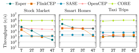
Figure 11. Throughput as a function of time-window size when using selection strategies.

In Figure 11, we display the throughput, separated by dataset, of each system running with a selection strategy. From here, we can conclude that the use of a selection strategy improves the performance of Esper, SASE, and OpenCEP. Esper still suffers with the time windows size, decreasing its performance exponentially when the window size increases (e.g., Stock Market). SASE and OpenCEP do not incur on this cost, having a stable throughput and, moreover, increasing it up to $10^{3}$ and $10^{4}$, respectively. Despite this improvement, CORE’s throughput is at least two OOM above other systems (i.e., $10^{6}$ e/s) and stable when the window size increases. Therefore, we can conclude then that the advantage of CORE is in the evaluation algorithm rather than in the use of selection strategies.

References

- (1)
- sys ([n.d.]) [n.d.]. CORE Website. https://github.com/CORE-cer. Accessed on 2022-03-15.
- sma ([n.d.]) [n.d.]. DEBS 2014 Grand Challenge: Smart homes. https://debs.org/grand-challenges/2014/. Accessed on 2022-03-11.
- tax ([n.d.]) [n.d.]. DEBS 2015 Grand Challenge: Taxi Trips. https://debs.org/grand-challenges/2015/. Accessed on 2022-03-11.
- Esp ([n.d.]) [n.d.]. Esper Enterprise Edition website. http://www.espertech.com/. Accessed on 2021-10-30.
- Fli ([n.d.]) [n.d.]. FlinkCEP - Complex event processing for Flink. https://ci.apache.org/projects/flink/flink-docs-release-1.13/docs/libs/cep/. Accessed on 2021-10-30.
- Ope ([n.d.]) [n.d.]. OpenCEP. https://research.redhat.com/blog/research_project/complex-event-processing-2/. Accessed on 2022-03-11.
- Sid ([n.d.]) [n.d.]. Siddhi: Cloud Native Stream Processor. https://siddhi.io/. Accessed on 2021-10-30.
- sto ([n.d.]) [n.d.]. Stock market data traces. https://davis.wpi.edu/datasets/Stock_Trace_Data/. Accessed on 2022-03-11.
- Agrawal et al. (2008) Jagrati Agrawal, Yanlei Diao, Daniel Gyllstrom, and Neil Immerman. 2008. Efficient pattern matching over event streams. In Proceedings of the 2008 ACM SIGMOD international conference on Management of data. Association for Computing Machinery, New York, NY, USA, 147–160.
- Aho and Hopcroft (1974) Alfred V Aho and John E Hopcroft. 1974. The design and analysis of computer algorithms. Pearson Education India.
- Alevizos et al. (2017) Elias Alevizos, Anastasios Skarlatidis, Alexander Artikis, and Georgios Paliouras. 2017. Probabilistic complex event recognition: A survey. ACM Computing Surveys (CSUR) 50, 5 (2017), 1–31.
- Amarilli et al. (2017) Antoine Amarilli, Pierre Bourhis, Louis Jachiet, and Stefan Mengel. 2017. A Circuit-Based Approach to Efficient Enumeration. In ICALP 2017-44th International Colloquium on Automata, Languages, and Programming. 1–15.
- Amarilli et al. (2019) Antoine Amarilli, Pierre Bourhis, Stefan Mengel, and Matthias Niewerth. 2019. Enumeration on trees with tractable combined complexity and efficient updates. In Proceedings of the 38th ACM SIGMOD-SIGACT-SIGAI Symposium on Principles of Database Systems. 89–103.
- Amarilli et al. (2021) Antoine Amarilli, Pierre Bourhis, Stefan Mengel, and Matthias Niewerth. 2021. Constant-delay enumeration for nondeterministic document spanners. ACM Transactions on Database Systems (TODS) 46, 1 (2021), 1–30.
- Anicic et al. (2010) Darko Anicic, Paul Fodor, Sebastian Rudolph, Roland Stühmer, Nenad Stojanovic, and Rudi Studer. 2010. A rule-based language for complex event processing and reasoning. In International Conference on Web Reasoning and Rule Systems. Springer, 42–57.
- Artikis et al. (2017a) Alexander Artikis, Nikos Katzouris, Ivo Correia, Chris Baber, Natan Morar, Inna Skarbovsky, Fabiana Fournier, and Georgios Paliouras. 2017a. A prototype for credit card fraud management: Industry paper. In Proceedings of the 11th ACM international conference on distributed and event-based systems. 249–260.
- Artikis et al. (2017b) Alexander Artikis, Alessandro Margara, Martin Ugarte, Stijn Vansummeren, and Matthias Weidlich. 2017b. Complex event recognition languages: Tutorial. In Proceedings of the 11th ACM International Conference on Distributed and Event-based Systems. 7–10.
- Artikis et al. (2014) Alexander Artikis, Marek Sergot, and Georgios Paliouras. 2014. An event calculus for event recognition. IEEE Transactions on Knowledge and Data Engineering 27, 4 (2014), 895–908.
- Artikis et al. (2012) Alexander Artikis, Anastasios Skarlatidis, François Portet, and Georgios Paliouras. 2012. Logic-based event recognition. The Knowledge Engineering Review 27, 4 (2012), 469–506.
- Bagan et al. (2007) Guillaume Bagan, Arnaud Durand, and Etienne Grandjean. 2007. On acyclic conjunctive queries and constant delay enumeration. In International Workshop on Computer Science Logic. Springer, 208–222.
- Berkholz et al. (2017) Christoph Berkholz, Jens Keppeler, and Nicole Schweikardt. 2017. Answering conjunctive queries under updates. In Proceedings of the 36th ACM SIGMOD-SIGACT-SIGAI Symposium on Principles of Database Systems. 303–318.
- Carmeli and Kröll (2021) Nofar Carmeli and Markus Kröll. 2021. On the Enumeration Complexity of Unions of Conjunctive Queries. ACM Transactions on Database Systems (TODS) 46, 2 (2021), 1–41.
- Chesani et al. (2010) Federico Chesani, Paola Mello, Marco Montali, and Paolo Torroni. 2010. A logic-based, reactive calculus of events. Fundamenta Informaticae 105, 1-2 (2010), 135–161.
- Cugola and Margara (2010) Gianpaolo Cugola and Alessandro Margara. 2010. TESLA: a formally defined event specification language. In Proceedings of the Fourth ACM International Conference on Distributed Event-Based Systems. 50–61.
- Cugola and Margara (2012a) Gianpaolo Cugola and Alessandro Margara. 2012a. Complex event processing with T-REX. Journal of Systems and Software 85, 8 (2012), 1709–1728.
- Cugola and Margara (2012b) Gianpaolo Cugola and Alessandro Margara. 2012b. Processing flows of information: From data stream to complex event processing. ACM Computing Surveys (CSUR) 44, 3 (2012), 1–62.
- Demers et al. (2005) Alan Demers, Johannes Gehrke, Mingsheng Hong, Mirek Riedewald, and Walker White. 2005. A general algebra and implementation for monitoring event streams. Technical Report. Cornell University.
- Demers et al. (2006) Alan Demers, Johannes Gehrke, Mingsheng Hong, Mirek Riedewald, and Walker White. 2006. Towards expressive publish/subscribe systems. In International Conference on Extending Database Technology. Springer, 627–644.
- Florenzano et al. (2020) Fernando Florenzano, Cristian Riveros, Martín Ugarte, Stijn Vansummeren, and Domagoj Vrgoč. 2020. Efficient enumeration algorithms for regular document spanners. ACM Transactions on Database Systems (TODS) 45, 1 (2020), 1–42.
- Giatrakos et al. (2020) Nikos Giatrakos, Elias Alevizos, Alexander Artikis, Antonios Deligiannakis, and Minos Garofalakis. 2020. Complex event recognition in the big data era: a survey. The VLDB Journal 29, 1 (2020), 313–352.
- Grez et al. (2019) Alejandro Grez, Cristian Riveros, and Martín Ugarte. 2019. A formal framework for complex event processing. In 22nd International Conference on Database Theory (ICDT 2019). Schloss Dagstuhl-Leibniz-Zentrum fuer Informatik, 5:1–5:18.
- Grez et al. (2020) Alejandro Grez, Cristian Riveros, Martín Ugarte, and Stijn Vansummeren. 2020. On the expressiveness of languages for complex event recognition. In 23rd International Conference on Database Theory (ICDT 2020). Schloss Dagstuhl-Leibniz-Zentrum für Informatik, 15:1–15:17.
- Grez et al. (2021) Alejandro Grez, Cristian Riveros, Martin Ugarte, and Stijn Vansummeren. 2021. A Formal Framework for Complex Event Recognition. ACM Transactions on Database Systems (TODS) (2021). https://doi.org/10.1145/3485463 To appear.
- Groover (2007) Mikell P Groover. 2007. Automation, production systems, and computer-integrated manufacturing. Prentice Hall.
- Hirzel (2012) Martin Hirzel. 2012. Partition and compose: Parallel complex event processing. In DEBS. 191–200.
- Idris et al. (2020) Muhammad Idris, Martín Ugarte, Stijn Vansummeren, Hannes Voigt, and Wolfgang Lehner. 2020. General dynamic Yannakakis: conjunctive queries with theta joins under updates. The VLDB Journal 29, 2 (2020), 619–653.
- Kolchinsky and Schuster (2018) Ilya Kolchinsky and Assaf Schuster. 2018. Efficient Adaptive Detection of Complex Event Patterns. Proc. VLDB Endow. 11, 11 (2018), 1346–1359. https://doi.org/10.14778/3236187.3236190
- Kolchinsky et al. (2015) Ilya Kolchinsky, Izchak Sharfman, and Assaf Schuster. 2015. Lazy evaluation methods for detecting complex events. In Proceedings of the 9th ACM International Conference on Distributed Event-Based Systems, DEBS ’15, Oslo, Norway, June 29 - July 3, 2015, Frank Eliassen and Roman Vitenberg (Eds.). ACM, 34–45. https://doi.org/10.1145/2675743.2771832
- Liu et al. (2011) Mo Liu, Elke Rundensteiner, Kara Greenfield, Chetan Gupta, Song Wang, Ismail Ari, and Abhay Mehta. 2011. E-cube: multi-dimensional event sequence analysis using hierarchical pattern query sharing. In Proceedings of the 2011 ACM SIGMOD International Conference on Management of data. 889–900.
- Mayer et al. (2017) Ruben Mayer, Muhammad Adnan Tariq, and Kurt Rothermel. 2017. Minimizing communication overhead in window-based parallel complex event processing. In Proceedings of the 11th ACM International Conference on Distributed and Event-based Systems. 54–65.
- Mei and Madden (2009) Yuan Mei and Samuel Madden. 2009. Zstream: a cost-based query processor for adaptively detecting composite events. In Proceedings of the 2009 ACM SIGMOD International Conference on Management of data. 193–206.
- Mukherjee et al. (1994) Biswanath Mukherjee, L Todd Heberlein, and Karl N Levitt. 1994. Network intrusion detection. IEEE network 8, 3 (1994), 26–41.
- Pietzuch et al. (2003) Peter R Pietzuch, Brian Shand, and Jean Bacon. 2003. A framework for event composition in distributed systems. In ACM/IFIP/USENIX International Conference on Distributed Systems Platforms and Open Distributed Processing. Springer, 62–82.
- Pitsikalis et al. (2019) Manolis Pitsikalis, Alexander Artikis, Richard Dreo, Cyril Ray, Elena Camossi, and Anne-Laure Jousselme. 2019. Composite event recognition for maritime monitoring. In Proceedings of the 13th ACM International Conference on Distributed and Event-based Systems. 163–174.
- Poppe et al. (2017a) Olga Poppe, Chuan Lei, Salah Ahmed, and Elke A Rundensteiner. 2017a. Complete event trend detection in high-rate event streams. In Proceedings of the 2017 ACM International Conference on Management of Data. 109–124.
- Poppe et al. (2021) Olga Poppe, Chuan Lei, Lei Ma, Allison Rozet, and Elke A Rundensteiner. 2021. To share, or not to share online event trend aggregation over bursty event streams. In Proceedings of the 2021 International Conference on Management of Data. 1452–1464.
- Poppe et al. (2017b) Olga Poppe, Chuan Lei, Elke A Rundensteiner, and David Maier. 2017b. GRETA: graph-based real-time event trend aggregation. Proceedings of the VLDB Endowment 11, 1 (2017), 80–92.
- Poppe et al. (2019) Olga Poppe, Chuan Lei, Elke A Rundensteiner, and David Maier. 2019. Event trend aggregation under rich event matching semantics. In Proceedings of the 2019 International Conference on Management of Data. 555–572.
- Ray et al. (2016) Medhabi Ray, Chuan Lei, and Elke A Rundensteiner. 2016. Scalable pattern sharing on event streams. In Proceedings of the 2016 international conference on management of data. 495–510.
- Sahay and Ranjan (2008) BS Sahay and Jayanthi Ranjan. 2008. Real time business intelligence in supply chain analytics. Information Management & Computer Security 16 (2008), 28–48.
- Schultz-Møller et al. (2009) Nicholas Poul Schultz-Møller, Matteo Migliavacca, and Peter Pietzuch. 2009. Distributed complex event processing with query rewriting. In Proceedings of the Third ACM International Conference on Distributed Event-Based Systems. 1–12.
- Segoufin (2013) Luc Segoufin. 2013. Enumerating with constant delay the answers to a query. In Proceedings of the 16th International Conference on Database Theory. 10–20.
- Suhothayan et al. (2011) Sriskandarajah Suhothayan, Kasun Gajasinghe, Isuru Loku Narangoda, Subash Chaturanga, Srinath Perera, and Vishaka Nanayakkara. 2011. Siddhi: A second look at complex event processing architectures. In Proceedings of the 2011 ACM workshop on Gateway computing environments. 43–50.
- Vardi (1982) Moshe Y Vardi. 1982. The complexity of relational query languages. In Proceedings of the fourteenth annual ACM symposium on Theory of computing. 137–146.
- Wu et al. (2006) Eugene Wu, Yanlei Diao, and Shariq Rizvi. 2006. High-performance complex event processing over streams. In Proceedings of the 2006 ACM SIGMOD international conference on Management of data. 407–418.
- Zhang et al. (2014) Haopeng Zhang, Yanlei Diao, and Neil Immerman. 2014. On complexity and optimization of expensive queries in complex event processing. In Proceedings of the 2014 ACM SIGMOD international conference on Management of data. 217–228.
- Zhang et al. (2017) Shuhao Zhang, Hoang Tam Vo, Daniel Dahlmeier, and Bingsheng He. 2017. Multi-query optimization for complex event processing in SAP ESP. In 2017 IEEE 33rd International Conference on Data Engineering (ICDE). IEEE, 1213–1224.
- Zhao et al. (2020) Bo Zhao, Nguyen Quoc Viet Hung, and Matthias Weidlich. 2020. Load shedding for complex event processing: Input-based and state-based techniques. In 2020 IEEE 36th International Conference on Data Engineering (ICDE). IEEE, 1093–1104.
- Zhao et al. (2021) Bo Zhao, Han van der Aa, Thanh Tam Nguyen, Quoc Viet Hung Nguyen, and Matthias Weidlich. 2021. EIRES: Efficient Integration of Remote Data in Event Stream Processing. In Proceedings of the 2021 International Conference on Management of Data. 2128–2141.