Strong convergence rate of Euler–Maruyama approximations in temporal-spatial Hölder-norms

Abstract

Classical approximation results for stochastic differential equations analyze the $L^{p}$-distance between the exact solution and its Euler–Maruyama approximations. In this article we measure the error with temporal-spatial Hölder-norms. Our motivation for this are multigrid approximations of the exact solution viewed as a function of the starting point. We establish the classical strong convergence rate $0.5$ with respect to temporal-spatial Hölder-norms if the coefficient functions have bounded derivatives of first and second order.

1 Introduction

Stochastic differential equations are typically not explicitly solvable and need to be approximated numerically. Classical results on strong convergence rates assume the SDE coefficients to be globally Lipschitz continuous; see, e.g., [18, 21]. In the last decade, strong convergence rates were also established in the case of non-globally Lipschitz coefficients. We refer, e.g., to [10, 11, 13, 27, 28] for the case of locally Lipschitz coefficients with polynomial growth where Euler approximations diverge in the strong and weak sense; see [12, 14]. Moreover, we refer, e.g., to [1, 4, 19, 20, 22, 23, 24] for the case of discontinuous drift coefficients. The error is measured in all of these approximation results as $L^{p}$-distance between the exact solution and the approximations for at least one $p\in[1,\infty)$.

In this article we measure the error with temporal-spatial Hölder-norms. Our motivation for considering spatial Hölder-norms is that in a number of applications we need to approximate the solution in several starting points, e.g., in a domain or a submanifold. It is inefficient to approximate the exact solution (as a function of the starting point) by interpolating over a fine subgrid. More efficient is to apply multigrid approximations and to exploit the spatial regularity of the approximation processes. To give a specific example, the (first component of the) solution of a backward stochastic differential equation (BSDE) can be written as $(u(t,X_{t}))_{t\in[0,1]}$ where $X$ is the forward process and where $u$ solves a backward partial differential equation (PDE). Assuming that the PDE is linear, we can approximate $u$ by Monte Carlo Euler approximations $(U_{n})_{n\in{\mathbbm{N}}}$. It is inefficient to approximate $(u(t,X_{t}))_{t\in[0,1]}$ by an affine-linear interpolation of $(U^{n}(k2^{-n},X_{k2^{-n}}))_{k\in\{0,1,\ldots,2^{n}\}}$, $n\in{\mathbbm{N}}$. More efficient than this are multigrid approximations

$$\begin{split}\sum_{\ell=0}^{n-1}\Bigl{[}\mathscr{L}\big{(}(U^{n-\ell}(k2^{-\ell-1},X_{k2^{-\ell-1}}))_{k\in\{0,1,\ldots,2^{\ell+1}\}}\big{)}-\mathbbm{1}_{{\mathbbm{N}}}(\ell)\mathscr{L}\big{(}(U^{n-\ell}(k2^{-\ell},X_{k2^{-\ell}}))_{k\in\{0,1,\ldots,2^{\ell}\}}\big{)}\Bigr{]}\end{split}$$ (1)

where $\mathbbm{1}_{{\mathbbm{N}}}$ is the indicator function of ${\mathbbm{N}}=\{1,2,\ldots\}$ and for every $N\in{\mathbbm{N}}$, $a\colon\{0,1,,\ldots,N\}\to{\mathbbm{R}}$ we denote by $\mathscr{L}(a)\in C([0,1],{\mathbbm{R}})$ the continuous function which satisfies for all $k\in\{0,1,\ldots,N-1\}$, $t\in[\frac{k}{N},\frac{k+1}{N}]$ that $(\mathscr{L}(a))(t)=a_{k}(k+1-Nt)+a_{k+1}(Nt-k)$; see [16, Theorem 2.3] for more details and cf. also [7, 8]. For the analysis of these multigrid approximations, however, we need to understand the temporal-spatial regularity of Monte Carlo Euler approximations. If the PDE is nonlinear and high-dimensional, then we can approximate its solution by multilevel Picard approximations; see, e.g., [5, 17, 15]. Also in this case we need to understand regularity of Euler–Maruyama approximations considered as functions of the starting point.

The following Theorem 1.1 illustrates the main result of this article and proves that Euler–Maruyama approximations converge with strong convergence rate $0.5$ also in spatial $1$-Hölder norms under suitable assumptions. The central assumption of Theorem 1.1 is that the coefficient functions $\mu$ and $\sigma$ are twice continuously differentiable and that the derivatives of first and second order are bounded. In fact, it suffices to assume a weaker assumption on the coefficient functions, namely there exists $c\in{\mathbbm{R}}$ such that for all $\zeta\in\{\mu,\sigma\}$, $x,y\in{\mathbbm{R}}^{d}$ it holds that

$$\begin{split}&\left\lVert(\zeta(x)-\zeta(y))-(\zeta(\tilde{x})-\zeta(\tilde{y}))\right\rVert\leq c\left\lVert(x-y)-(\tilde{x}-\tilde{y})\right\rVert+c\left(\left\lVert x-y\right\rVert+\left\lVert\tilde{x}-\tilde{y}\right\rVert\right)\lVert x-\tilde{x}\rVert,\end{split}$$ (2)

cf. Theorem 3.2 for details. So global Lipschitz continuity of the coefficient functions is sufficient for Euler–Maruyama approximations to converge with strong convergence rate $0.5$ whereas condition (LABEL:eq:second.order) is sufficient to obtain strong convergence rate $0.5$ with respect to spatial Hölder norms. Clearly, (LABEL:eq:second.order) implies global Lipschitz continuity of $\mu$ and $\sigma$. We believe, however, that condition (LABEL:eq:second.order) is not necessary for (3) to hold. It would be interesting to prove convergence rates in strong spatial Hölder norms in the situations considered in the articles mentioned in the first paragraph, that is, when the coefficients are only locally Lipschitz continuous or when the drift coefficient is only measurable (plus suitable additional assumptions).

Theorem 1.1.

Let $d\in{\mathbbm{N}}$, $T,p\in(0,\infty)$, let $\lVert\cdot\rVert\colon{\mathbbm{R}}^{d}\to[0,\infty)$ be a norm, let $\mu\in C^{2}({\mathbbm{R}}^{d},{\mathbbm{R}}^{d})$, $\sigma\in C^{2}({\mathbbm{R}}^{d},{\mathbbm{R}}^{d\times d})$ have bounded first and second order derivatives, let $(\Omega,\mathcal{F},{\mathbbm{P}},({\mathbbm{F}}_{t})_{t\in[0,T]})$ be a filtered probability space which satisfies the usual conditions, let $(W_{t})_{t\in[0,T]}\colon[0,T]\times\Omega\to{\mathbbm{R}}^{d}$ be a standard $({\mathbbm{F}}_{t})_{t\in[0,T]}$-Brownian motion with continuous sample paths, and for every $n\in{\mathbbm{N}}$, $x\in{\mathbbm{R}}^{d}$ let ${Y}_{k}^{n,x}\colon\Omega\to{\mathbbm{R}}^{d}$, $k\in\{0,\ldots,n\}$, satisfy for all $k\in\{0,\ldots,n-1\}$ that ${Y}_{0}^{n,x}=x$ and ${Y}_{k+1}^{n,x}={Y}_{k}^{n,x}+\mu({Y}_{k}^{n,x})\tfrac{T}{n}+\sigma({Y}_{k}^{n,x})(W_{\frac{(k+1)T}{n}}-W_{\frac{kT}{n}}).$ Then

1. for every $x\in{\mathbbm{R}}^{d}$ there exists a unique adapted stochastic process with continuous sample paths $(X^{x}_{t})_{t\in[0,T]}\colon[0,T]\times\Omega\to{\mathbbm{R}}^{d}$ such that for all $t\in[0,T]$ it holds a.s. that $X_{t}^{x}=x+\int_{0}^{t}\mu(X_{s}^{x})\,ds+\int_{0}^{t}\sigma(X_{s}^{x})\,dW_{s}$ and

2. there exists $C\in[0,\infty)$ which satisfies for all $n\in{\mathbbm{N}}$, $k\in\{0,1,\ldots,n\}$, $x\in{\mathbbm{R}}^{d}$, $y\in{\mathbbm{R}}^{d}\setminus\{x\}$ that

   $$\begin{split}\frac{\left({\mathbbm{E}}\!\left[\bigl{\lVert}X_{\frac{kT}{n}}^{x}-{Y}_{k}^{n,x}\bigr{\rVert}^{p}\right]\right)^{1/p}}{1+\lVert x\rVert}+\frac{\left({\mathbbm{E}}\!\left[\bigl{\lVert}\bigl{(}X_{\frac{kT}{n}}^{x}-{Y}_{k}^{n,x}\bigr{)}-\bigl{(}X_{\frac{kT}{n}}^{y}-{Y}_{k}^{n,y}\bigr{)}\bigr{\rVert}^{p}\right]\right)^{1/p}}{\lVert x-y\rVert\bigl{(}1+\lVert x\rVert+\lVert y\rVert\bigr{)}}\leq\frac{C}{\sqrt{n}}.\end{split}$$ (3)

Theorem 1.1 follows from Corollary 3.4, Hölder’s inequality, and the fact that for all $d\in{\mathbbm{N}}$ it holds that all norms on ${\mathbbm{R}}^{d}$ are equivalent. In order to illustrate Theorem 1.1 by a numerical experiment we consider an example where the SDE solution is explicit, Example 1.2 below.

Example 1.2.

Consider the setting of Theorem 1.1, assume for all $x\in{\mathbbm{R}}$ that $T=1$, $d=1$, $p=2$, $\mu(x)=-\sin(x)\cos^{3}(x)$, and $\sigma(x)=\cos^{2}(x)$ and for every $n\in{\mathbbm{N}}$ let $\Delta_{n}\in{\mathbbm{R}}$ satisfy that $\Delta_{n}=\bigl{(}{\mathbbm{E}}\bigl{[}\bigl{\lvert}(X_{1}^{1}-{Y}_{n}^{n,1})-(X_{1}^{1+\frac{1}{n}}-{Y}_{n}^{n,1+\frac{1}{n}})\bigr{\rvert}^{2}\bigr{]}\bigr{)}^{1/2}.$ We approximate each expectation by a Monte-Carlo average over $1000$ independent samples. Note that for all $t\in[0,1]$, $x\in{\mathbbm{R}}$ it holds a.s. that

$$X_{t}^{x}=x-\int_{0}^{t}\sin(X_{s}^{x})\cos^{3}(X_{s}^{x})\,ds+\int_{0}^{t}\cos^{2}(X^{x}_{s})\,dW_{s}$$ (4)

and $X_{t}^{x}=\arctan(aW_{t}+\tan(x))$ (see, e.g., [18, (4.27) in p. 121]). Theorem 1.1 shows that $\sup_{n\in{\mathbbm{N}}}[\Delta_{n}n^{-1.5}]<\infty$. Our simulations support this result and show that $(2^{n},\Delta_{2^{n}})_{n\in\{1,2,\ldots,10\}}$, decays like $(2^{n},(2^{n})^{-1.5})_{n\in\{1,2,\ldots,10\}}$; see Fig. 1.

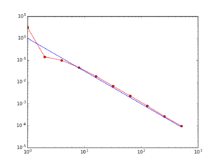
Figure 1: Simulation by Python using numpy and matplotlib.pyplot for Example 1.2. The line with dots contains the points $(2^{n},\Delta_{2^{n}})$ for $n\in\{1,2,\ldots,10\}$ in Example 1.2. The straight line is the reference line $(2^{n},(2^{n})^{-1.5})_{n\in\{1,2,\ldots,10\}}.$

The remainder of this article is organized as follows. In Section 2 we generalize Gronwall’s lemma to the case of general temporal discretizations. In Section 3 we prove under suitable assumptions that Euler–Maruyama approximations converge in temporal-spatial Hölder $L^{p}$-norms with rate $0.5$ (cf. Theorem 3.2 and Corollary 3.4). As a corollary hereof, we prove in Corollary 3.5 that Monte Carlo Euler approximations converge in spatial Lipschitz $L^{p}$-norms with rate $0.5$.

2 Gronwall inequalities

Lemma 2.1 generalizes the well-known discrete and continuous Gronwall lemma.

Lemma 2.1.

Let $a,c\in[0,\infty)$, $T\in{\mathbbm{R}}$, $t_{0}\in(-\infty,T)$, let $x\colon[t_{0},T]\to[0,\infty)$, $\delta\colon[t_{0},T]\to[t_{0},T]$ be measurable, and assume for all $t\in[t_{0},T]$ that $\delta(t)\leq t$ and $x(t)\leq a+\int_{t_{0}}^{t}cx(\delta(s))\,ds<\infty.$ Then for all $t\in[t_{0},T]$ it holds that $x(t)\leq ae^{c(t-t_{0})}$.

Proof of Lemma 2.1.

The assumptions on $x$ and $\delta$ imply for all $t\in[t_{0},T]$ that $x(\delta(t))\leq a+\int_{t_{0}}^{\delta(t)}cx(\delta(s))\,ds\leq a+\int_{t_{0}}^{t}cx(\delta(s))\,ds<\infty$. This and Gronwall’s lemma (see, e.g., [6, Lemma 2.11]) show for all $t\in[t_{0},T]$ that $x(\delta(t))\leq ae^{c(t-t_{0})}$. Therefore, the assumptions on $x$ and $\delta$ imply for all $t\in[t_{0},T]$ that $x(t)\leq a+\int_{t_{0}}^{t}cx(\delta(s))\,ds\leq a(1+c\int_{t_{0}}^{t}e^{c(s-t_{0})}\,ds)=ae^{c(t-t_{0})}.$ This completes the proof of Lemma 2.1. ∎

Corollary 2.2.

Let $c\in[0,\infty)$, $p\in[1,\infty)$, $T\in{\mathbbm{R}}$, $t_{0}\in(-\infty,T)$, let $a,x\colon[t_{0},T]\to[0,\infty)$, $\delta\colon[t_{0},T]\to[t_{0},T]$ be measurable, and assume for all $t\in[t_{0},T]$ that $\delta(t)\leq t$ and $x(t)\leq a(t)+\bigl{(}\int_{t_{0}}^{t}\lvert cx(\delta(s))\rvert^{p}\,ds\bigr{)}^{\nicefrac{{1}}{{p}}}<\infty.$ Then for all $t\in[t_{0},T]$ it holds that

$$\textstyle x(t)\leq 2^{1-\frac{1}{p}}\left[\sup_{s\in[t_{0},t]}a(s)\right]\exp(\tfrac{2^{p-1}c^{p}(t-t_{0})}{p}).$$ (5)

Proof of Corollary 2.2.

The assumptions and the fact that $\forall\,A,B\in[0,\infty)\colon(A+B)^{p}\leq 2^{p-1}(A^{p}+B^{p})$ show for all ${t}\in[t_{0},T]$, $\bar{t}\in[t,T]$ that $\lvert x(t)\rvert^{p}\leq 2^{p-1}\sup_{s\in[t_{0},\bar{t}]}a^{p}(s)+2^{p-1}\int_{t_{0}}^{t}c^{p}\lvert x(\delta(s))\rvert^{p}\,ds<\infty.$ This and Lemma 2.1 (applied for every $\bar{t}\in(t_{0},T]$ with $a\curvearrowleft 2^{p-1}\sup_{s\in[t_{0},\bar{t}]}a^{p}(s)$, $c\curvearrowleft 2^{p-1}c^{p}$, $T\curvearrowleft\bar{t}$, $x\curvearrowleft x^{p}|_{[t_{0},\bar{t}]}$ in the notation of Lemma 2.1) imply for all ${t}\in(t_{0},T]$, $\bar{t}\in[t,T]$ that $\lvert x(t)\rvert^{p}\leq 2^{p-1}\sup_{s\in[t_{0},\bar{t}]}a^{p}(s)\exp(2^{p-1}c^{p}(t-t_{0}))$. This and the fact that $x(t_{0})\leq a(t_{0})$ complete the proof of Corollary 2.2. ∎

3 Strong convergence rate of Euler–Maruyama approximations in temporal-spatial Hölder norms

In Section 3 we prove under suitable assumptions that Euler–Maruyama approximations converge in temporal-spatial Hölder $L^{p}$-norms with rate $0.5$ (cf. Theorem 3.2 and Corollary 3.4). As a corollary hereof, we prove in Corollary 3.5 that Monte Carlo Euler approximations converge in spatial Lipschitz $L^{p}$-norms with rate $0.5$. The central assumption for this is (9). In Lemma 3.3 below we provide the well-known fact that a $C^{2}$-function with bounded first and second order derivatives satisfies this condition (9). First, we provide in Lemma 3.1 well-known upper bounds for polynomials which we use as Lyapunov-type functions.

Lemma 3.1.

Let $d\in{\mathbbm{N}}$, let $\lVert\cdot\rVert\colon{\mathbbm{R}}^{d}\to[0,\infty)$ be the standard norm, and let $p\in[3/2,\infty)$, $a,c\in[0,\infty)$, $V\colon{\mathbbm{R}}^{d}\to{\mathbbm{R}}$ satisfy for all $x\in{\mathbbm{R}}^{d}$ that $V(x)=({a}+c^{2}\lVert x\rVert^{2})^{p}.$ Then it holds for all $x,y,z\in{\mathbbm{R}}^{d}$ that $\bigl{\lvert}((\mathsf{D}V)(x))(y)\bigr{\rvert}\leq 2pc(V(x))^{\frac{2p-1}{2p}}\lVert y\rVert$ and $\bigl{\lvert}((\mathsf{D}^{2}V)(x))(y,z)\bigr{\rvert}\leq 2p(2p-1)c^{2}(V(x))^{\frac{p-1}{p}}\lVert y\rVert\lVert z\rVert$.

Proof of Lemma 3.1.

Throughout the proof let $\langle\cdot,\cdot\rangle\colon{\mathbbm{R}}^{d}\times{\mathbbm{R}}^{d}\to{\mathbbm{R}}$ be the standard scalar product. The assumptions and the Cauchy-Schwarz inequality show for all $x,y,z\in{\mathbbm{R}}^{d}$ that $c\lVert x\rVert\leq(V(x))^{\frac{1}{2p}}$, $\bigl{\lvert}[(\mathsf{D}V)(x)](y)\bigr{\rvert}=\bigl{\lvert}p\bigl{[}{a}+c^{2}\lVert x\rVert^{2}\bigr{]}^{p-1}2c^{2}\langle x,y\rangle\bigr{\rvert}\leq 2pc^{2}(V(x))^{\frac{p-1}{p}}\lVert x\rVert\lVert y\rVert\leq 2pc(V(x))^{\frac{2p-1}{2p}}\lVert y\rVert,$ and

$$\begin{split}\left\lvert[(\mathsf{D}^{2}V)(x)](y,z)\right\rvert&=\left\lvert p(p-1)\left[{a}+c^{2}\lVert x\rVert^{2}\right]^{p-2}2c^{2}\langle x,z\rangle 2c^{2}\langle x,y\rangle+2pc^{2}\left[{a}+c^{2}\lVert x\rVert^{2}\right]^{p-1}\langle y,z\rangle\right\rvert\\ &\leq 4p(p-1)c^{4}(V(x))^{\frac{p-2}{p}}\lVert x\rVert^{2}\lVert y\rVert\lVert z\rVert+2pc^{2}(V(x))^{\frac{p-1}{p}}\lVert y\rVert\lVert z\rVert\\ &\leq 4p(p-1)c^{2}(V(x))^{\frac{p-1}{p}}\lVert y\rVert\lVert z\rVert+2pc^{2}(V(x))^{\frac{p-1}{p}}\lVert y\rVert\lVert z\rVert\\ &\leq(4p^{2}-2p)c^{2}(V(x))^{\frac{p-1}{p}}\lVert y\rVert\lVert z\rVert.\end{split}$$ (6)

This completes the proof of Lemma 3.1. ∎

The following theorem, Theorem 3.2, is the main result of this article and establishes strong convergence rate $0.5$ of Euler–Maruyama approximations in temporal-spatial Hölder norms. The estimates in Theorem 3.2 are explicit in all parameters. In particular, this allows to identify situations where the approximation error grows at most polynomially in the dimension and where the Euler–Maruyama approximations do not suffer from the curse of dimensionality. Note that $b=\infty$ is the case of globally Lipschitz continuous coefficients and in this case the right-hand sides of (16) and (17) are trivial (in $\{0,\infty\}$). Moreover, observe that (12) and the fact that $\forall\,t\in[0,T]\colon\iota(t)=t$ imply for every $s\in[0,T]$, $x\in{\mathbbm{R}}^{d}$ that $(X^{\iota,x}_{s,t})_{t\in[s,T]}$ is the exact solution to the SDE with coefficient functions $\mu,\sigma$ starting at $(s,x)$. Furthermore, (12) implies that for all $\delta\in\mathbbm{S}$, $n\in{\mathbbm{N}}$, $t_{0},t_{1},\ldots,t_{n}\in[0,T]$, $k\in[0,n-1]\cap{\mathbbm{Z}}$, $s\in[0,T]$, $t\in[s,T]$ with $0=t_{0}<t_{1}<\ldots<t_{n}=T$, $\delta([t_{0},t_{1}])=\{t_{0}\},\delta((t_{1},t_{2}])=\{t_{1}\},\ldots,\delta((t_{n-1},t_{n}])=\{t_{n-1}\}$, $t\in(t_{k},t_{k+1}]$ it holds that $\delta(t)=t_{k}$, $X_{s,s}^{\delta,x}=x$, and

$$X^{\delta,x}_{s,t}=X^{\delta,x}_{s,\max\{s,t_{k}\}}+\mu(X^{\delta,x}_{s,\max\{s,t_{k}\}})(t-\max\{s,t_{k}\})+\sigma(X^{\delta,x}_{s,\max\{s,t_{k}\}})(W_{t}-W_{\max\{s,t_{k}\}}),$$ (7)

that is, $(X^{\delta,x}_{s,t})_{t\in[s,T]}$ is the Euler–Maruyama approximation to the SDE with coefficient functions $\mu,\sigma$ starting at $(s,x)$ and associated to the partition $(t_{0},t_{1},\ldots,t_{n})$ of $[0,T]$.

Let us discuss the proof of Theorem 3.2. First, (i)–(iv) are standard results and we include their proofs here for convenience and to have explicit constants. The main parts of Theorem 3.2 are (v)–(vi). While the estimate of a two point term is based on Gronwall’s inequality and (27), the four point term in (v) is estimated by using Gronwall’s inequality and (44). A crucial step for (44) is (31) in which the regularity assumption of $\mu,\sigma$ in (9) is used to “break” the four point term containing $\mu,\sigma$ in (44) into a four point term solely containing the SDE solution and its approximation. To prove (vi) we extend the four point estimate in (v) to time regularity estimates. In the proof of (iii) we have done similar things but for two point terms.

Theorem 3.2 (Strong convergence of Euler–Maruyama approximations in Hölder norms).

Let $\lVert\cdot\rVert\colon\bigcup_{k,\ell\in{\mathbbm{N}}}{\mathbbm{R}}^{k\times\ell}\to[0,\infty)$ satisfy for all $k,\ell\in{\mathbbm{N}}$, $s=(s_{ij})_{i\in[1,k]\cap{\mathbbm{N}},j\in[1,\ell]\cap{\mathbbm{N}}}\in{\mathbbm{R}}^{k\times\ell}$ that $\lVert s\rVert^{2}=\sum_{i=1}^{k}\sum_{j=1}^{\ell}\lvert s_{ij}\rvert^{2}$, let $0\cdot\infty=0$, let $d,m\in{\mathbbm{N}}$, $T,c,\bar{c}\in(0,\infty)$, $b\in(0,\infty]$, $p\in[2,\infty)$, $\mu\in C({\mathbbm{R}}^{d},{\mathbbm{R}}^{d})$, $\sigma\in C({\mathbbm{R}}^{d},{\mathbbm{R}}^{d\times m})$, $V\in C^{2}({\mathbbm{R}}^{d},[1,\infty))$ satisfy for all $x,y,\tilde{x},\tilde{y}\in{\mathbbm{R}}^{d}$ that $\lVert\mu(0)\rVert+\lVert\sigma(0)\rVert+c\lVert x\rVert\leq(V(x))^{\nicefrac{{1}}{{p}}},$

$$\bigl{\lvert}((\mathsf{D}V)(x))(y)\bigr{\rvert}\leq\bar{c}(V(x))^{\frac{p-1}{p}}\lVert y\rVert,\quad\bigl{\lvert}((\mathsf{D}^{2}V)(x))(y,y)\bigr{\rvert}\leq\bar{c}(V(x))^{\frac{p-2}{p}}\lVert y\rVert^{2},$$ (8)

and

$$\begin{split}&\max_{\zeta\in\{\mu,\sigma\}}\left\lVert(\zeta(x)-\zeta(y))-(\zeta(\tilde{x})-\zeta(\tilde{y}))\right\rVert\\ &\leq c\left\lVert(x-y)-(\tilde{x}-\tilde{y})\right\rVert+b\frac{\left\lVert x-y\right\rVert+\left\lVert\tilde{x}-\tilde{y}\right\rVert}{2}\lVert x-\tilde{x}\rVert,\end{split}$$ (9)

let $\iota\colon[0,T]\to[0,T]$ satisfy for all $t\in[0,T]$ that $\iota(t)=t$, let $\mathbbm{S}$ satisfy that

$$\small\begin{split}\mathbbm{S}=\left\{\delta\colon[0,T]\to[0,T]\colon\begin{aligned} &\exists\,n\in{\mathbbm{N}},t_{0},t_{1},\ldots,t_{n}\in[0,T]\colon 0=t_{0}<t_{1}<\ldots<t_{n}=T,\\ &\delta([t_{0},t_{1}])=\{t_{0}\},\delta((t_{1},t_{2}])=\{t_{1}\},\ldots,\delta((t_{n-1},t_{n}])=\{t_{n-1}\}\end{aligned}\right\},\end{split}$$ (10)

let $\widetilde{\mathbbm{S}}=\mathbbm{S}\cup\{\iota\}$, let $\lvert\cdot\rvert\colon\widetilde{\mathbbm{S}}\to[0,T]$ satisfy for all $\delta\in\mathbbm{S}$ that $\lvert\iota\rvert=0$ and

$$\lvert\delta\rvert=\max\Bigl{\{}\lvert s-t\rvert\colon s,t\in\delta([0,T]),s<t,(s,t)\cap\delta([0,T])=\emptyset\Bigr{\}},$$ (11)

let $(\Omega,\mathcal{F},{\mathbbm{P}},({\mathbbm{F}}_{t})_{t\in[0,T]})$ be a filtered probability space which satisfies the usual conditions, for every $s\in[1,\infty)$, $k,\ell\in{\mathbbm{N}}$ and every random variable $\mathfrak{X}\colon\Omega\to{\mathbbm{R}}^{k\times\ell}$ let $\lVert\mathfrak{X}\rVert_{s}\in[0,\infty]$ satisfy that $\lVert\mathfrak{X}\rVert_{s}^{s}={\mathbbm{E}}[\lVert\mathfrak{X}\rVert^{s}]$, let $W=(W_{t})_{t\in[0,T]}\colon[0,T]\times\Omega\to{\mathbbm{R}}^{m}$ be a standard $({\mathbbm{F}}_{t})_{t\in[0,T]}$-Brownian motion with continuous sample paths, and for every $\delta\in\widetilde{\mathbbm{S}}$, $s\in[0,T]$, $x\in{\mathbbm{R}}^{d}$ let $(X^{\delta,x}_{s,t})_{t\in[s,T]}\colon[s,T]\times\Omega\to{\mathbbm{R}}^{d}$ be an adapted stochastic process with continuous sample paths such that for all $t\in[s,T]$ it holds a.s. that

$$X^{\delta,x}_{s,t}=x+\int_{s}^{t}\mu(X_{s,\max\{s,\delta(r)\}}^{\delta,x})\,d{r}+\int_{s}^{t}\sigma(X_{s,\max\{s,\delta(r)\}}^{\delta,x})\,dW_{r}.$$ (12)

Then

1. it holds for all $\delta\in\widetilde{\mathbbm{S}}$, $s\in[0,T]$, $t\in[s,T]$, $x\in{\mathbbm{R}}^{d}$ that ${\mathbbm{E}}\bigl{[}V(X_{s,t}^{\delta,x})\bigr{]}\leq e^{1.5\bar{c}\lvert t-s\rvert}V(x),$

2. it holds for all $\delta\in\widetilde{\mathbbm{S}}$, $s\in[0,T]$, $t\in[s,T]$, $x\in{\mathbbm{R}}^{d}$ that

   $$\left\lVert X_{s,t}^{\delta,x}-X_{s,t}^{\iota,x}\right\rVert_{p}\leq\sqrt{2}c\left[\sqrt{T}+p\right]^{2}e^{c^{2}\left[\sqrt{T}+p\right]^{2}T}(e^{1.5\bar{c}T}V(x))^{\nicefrac{{1}}{{p}}}\lvert t-s\rvert^{\nicefrac{{1}}{{2}}}\lvert\delta\rvert^{\nicefrac{{1}}{{2}}},$$ (13)

3. it holds for all $\delta\in\widetilde{\mathbbm{S}}$, $s,\tilde{s}\in[0,T]$, $t\in[s,T]$, $\tilde{t}\in[\tilde{s},T]$, $x,\tilde{x}\in{\mathbbm{R}}^{d}$ that

   $$\begin{split}&\left\lVert X^{\delta,x}_{s,t}-X^{\delta,\tilde{x}}_{\tilde{s},\tilde{t}}\right\rVert_{p}\leq\sqrt{2}\lVert x-\tilde{x}\rVert e^{c^{2}\left[\sqrt{T}+p\right]^{2}T}\\ &+{5}e^{c^{2}\left[\sqrt{T}+p\right]^{2}T}\left[\sqrt{T}+p\right]e^{1.5\bar{c}T/p}\frac{(V(x))^{\nicefrac{{1}}{{p}}}+(V(\tilde{x}))^{\nicefrac{{1}}{{p}}}}{2}\left[\lvert s-\tilde{s}\rvert^{\nicefrac{{1}}{{2}}}+\lvert t-\tilde{t}\rvert^{\nicefrac{{1}}{{2}}}\right],\end{split}$$ (14)

4. it holds for all $\delta\in\widetilde{\mathbbm{S}}$, $s\in[0,T]$, $t,\tilde{t}\in[s,T]$, $x,\tilde{x}\in{\mathbbm{R}}^{d}$ that

   $$\left\lVert\bigl{(}X^{\delta,x}_{s,\tilde{t}}-X_{s,t}^{\delta,x}\bigr{)}-\bigl{(}X^{\delta,\tilde{x}}_{s,\tilde{t}}-X^{\delta,\tilde{x}}_{s,t}\bigr{)}\right\rVert_{p}\leq c\left[\sqrt{T}+p\right]\sqrt{2}e^{c^{2}\left[\sqrt{T}+p\right]^{2}T}\lVert x-\tilde{x}\rVert\lvert t-\tilde{t}\rvert^{\nicefrac{{1}}{{2}}},$$ (15)

5. it holds for all $\delta\in\widetilde{\mathbbm{S}}$, $s\in[0,T]$, $t\in[s,T]$, $x,\tilde{x},y,\tilde{y}\in{\mathbbm{R}}^{d}$ that

   $$\mathbbm{1}_{[4,\infty)}(p)\left\lVert\bigl{(}X^{\iota,x}_{s,t}-X^{\delta,y}_{s,t}\bigr{)}-\bigl{(}X^{\iota,\tilde{x}}_{s,t}-X^{\delta,\tilde{y}}_{s,t}\bigr{)}\right\rVert_{\frac{p}{2}}\leq\sqrt{2}e^{c^{2}\left[\sqrt{T}+p\right]^{2}T}\left\lVert\bigl{(}x-y\bigr{)}-\bigl{(}\tilde{x}-\tilde{y}\bigr{)}\right\rVert$$

   $$+2\sqrt{2}(c^{2}+bc+b)\left[\sqrt{T}+p\right]^{4}e^{3c^{2}\left[\sqrt{T}+p\right]^{2}T}e^{1.5\bar{c}T/p}\frac{(V(x))^{\nicefrac{{1}}{{p}}}+(V(\tilde{x}))^{\nicefrac{{1}}{{p}}}}{2}\lvert\delta\rvert^{\nicefrac{{1}}{{2}}}\lVert x-\tilde{x}\rVert\lvert t-s\rvert^{\nicefrac{{1}}{{2}}}$$

   $$+2\sqrt{2}b\left[\sqrt{T}+p\right]e^{3c^{2}\left[\sqrt{T}+p\right]^{2}T}\frac{\left(\lVert x-y\rVert+\lVert\tilde{x}-\tilde{y}\rVert\right)\lVert x-\tilde{x}\rVert}{2}\lvert t-s\rvert^{\nicefrac{{1}}{{2}}},$$ (16)

   and

6. it holds for all $\delta\in\widetilde{\mathbbm{S}}$, $s,\tilde{s}\in[0,T]$, $t\in[s,T]$, $\tilde{t}\in[\tilde{s},T]$, $x,\tilde{x}\in{\mathbbm{R}}^{d}$ that

   $$\begin{split}&\mathbbm{1}_{[4,\infty)}(p)\left\lVert\bigl{(}X_{s,t}^{\iota,x}-X_{\tilde{s},\tilde{t}}^{\iota,\tilde{x}}\bigr{)}-\bigl{(}X_{s,t}^{\delta,x}-X_{\tilde{s},\tilde{t}}^{\delta,\tilde{x}}\bigr{)}\right\rVert_{\frac{p}{2}}\\ &\leq 31(b+c)(c+1)\left[\sqrt{T}+p\right]^{6}e^{5c^{2}\left[\sqrt{T}+p\right]^{2}T}\\ &\qquad\qquad e^{4.5\bar{c}T/p}\frac{(V(x))^{\nicefrac{{2}}{{p}}}+(V(\tilde{x}))^{\nicefrac{{2}}{{p}}}}{2}\left[\lvert s-\tilde{s}\rvert^{\nicefrac{{1}}{{2}}}+\lvert t-\tilde{t}\rvert^{\nicefrac{{1}}{{2}}}+\lVert x-\tilde{x}\rVert\right]\lvert\delta\rvert^{\nicefrac{{1}}{{2}}}.\end{split}$$ (17)

Proof of Theorem 3.2.

Throughout this proof let $\sigma_{1},\sigma_{2},\ldots,\sigma_{m}\in C({\mathbbm{R}}^{d},{\mathbbm{R}}^{d})$ satisfy that $\sigma=(\sigma_{1},\sigma_{2},\ldots,\sigma_{m})$. First, observe that (9) (applied with $(x,y,\tilde{x},\tilde{y})\curvearrowleft(x,y,x,x)$ in the notation of (9)), the fact that $\forall\,x\in{\mathbbm{R}}^{d}\colon\lVert\mu(0)\rVert+\lVert\sigma(0)\rVert+c\lVert x\rVert\leq(V(x))^{\nicefrac{{1}}{{p}}}$, and the triangle inequality prove for all $x,y\in{\mathbbm{R}}^{d}$, $\zeta\in\{\mu,\sigma\}$ that

$$\left\lVert\zeta(x)-\zeta(y)\right\rVert\leq c\lVert x-y\rVert\quad\text{and}\quad\lVert\zeta(x)\rVert\leq\lVert\zeta(0)\rVert+c\lVert x\rVert\leq(V(x))^{\nicefrac{{1}}{{p}}}.$$ (18)

This, (8), and the fact that $\forall\,A,B\in[0,\infty),\lambda\in(0,1)\colon A^{\lambda}B^{1-\lambda}\leq\lambda A+(1-\lambda)B$ imply for all $x,y\in{\mathbbm{R}}^{d}$ that

$$\left\lvert((\mathsf{D}V)(y))(\mu(x))\right\rvert+\frac{1}{2}\left\lvert\sum_{k=1}^{m}((\mathsf{D}^{2}V)(y))(\sigma_{k}(x),\sigma_{k}(x))\right\rvert$$

$$\leq\bar{c}(V(y))^{1-\frac{1}{p}}\lVert\mu(x)\rVert+\frac{1}{2}\bar{c}(V(y))^{1-\frac{2}{p}}\lVert\sigma(x)\rVert^{2}$$

$$\leq\bar{c}(V(y))^{1-\frac{1}{p}}(V(x))^{\frac{1}{p}}+\frac{1}{2}\bar{c}(V(y))^{1-\frac{2}{p}}(V(x))^{\frac{2}{p}}$$

$$\leq\bar{c}\left[\left(1-\frac{1}{p}\right)V(y)+\frac{1}{p}V(x)\right]+\frac{1}{2}\bar{c}\left[\left(1-\frac{2}{p}\right)V(y)+\frac{2}{p}V(x)\right]$$

$$=\left[\bar{c}\left(1-\frac{1}{p}\right)+\frac{1}{2}\bar{c}\left(1-\frac{2}{p}\right)\right]V(y)+\left[\bar{c}\frac{1}{p}+\frac{1}{2}\bar{c}\frac{2}{p}\right]V(x)$$

$$=\left(1.5\bar{c}-\frac{2\bar{c}}{p}\right)V(y)+\frac{2\bar{c}}{p}V(x).$$ (19)

This and [2, Lemma 2.2] (applied for all $s\in[0,T)$, $t\in(s,T]$, $x\in{\mathbbm{R}}^{d}$ with $T\curvearrowleft t-s$, $O\curvearrowleft{\mathbbm{R}}^{d}$, $V\curvearrowleft\bigl{(}[0,t-s]\times{\mathbbm{R}}^{d}\ni(\mathfrak{t},\mathfrak{x})\mapsto V(\mathfrak{x})\in[0,\infty)\bigr{)}$, $\alpha\curvearrowleft\bigl{(}[0,t-s]\ni\mathfrak{t}\mapsto 1.5\bar{c}\in[0,\infty)\bigr{)}$, $\tau\curvearrowleft t-s$, $X\curvearrowleft(X^{\iota,x}_{s,s+r})_{r\in[0,t-s]}$ in the notation of [2, Lemma 2.2]) show for all $x\in{\mathbbm{R}}^{d}$, $s\in[0,T]$, $t\in[s,T]$ that

$${\mathbbm{E}}\bigl{[}V(X_{s,t}^{\iota,x})\bigr{]}\leq e^{1.5\bar{c}(t-s)}V(x).$$ (20)

Next, (19), [9, Theorem 2.4] (applied for all $x\in{\mathbbm{R}}^{d}$, $s\in[0,T]$ with $H\curvearrowleft{\mathbbm{R}}^{d}$, $U\curvearrowleft{\mathbbm{R}}^{m}$, $O\curvearrowleft{\mathbbm{R}}^{d}$, $\tau\curvearrowleft(\Omega\ni\omega\mapsto s\in[0,T])$, $X\curvearrowleft(x+\mu(x)t+\sigma(x)W_{t})_{{t}\in[0,T]}$, $a\curvearrowleft\bigl{(}[0,T]\times\Omega\ni({t},\omega)\mapsto\mu(x)\in{\mathbbm{R}}^{d}\bigr{)}$, $b\curvearrowleft\bigl{(}[0,T]\times\Omega\ni(t,\omega)\mapsto\sigma(x)\in{\mathbbm{R}}^{{d\times m}}\bigr{)}$, $p\curvearrowleft 1$, $V\curvearrowleft([0,T]\times{\mathbbm{R}}^{d}\ni(t,y))\mapsto V(y)\in[0,\infty))$, $\alpha\curvearrowleft\bigl{(}[0,T]\times\Omega\ni({t},\omega)\mapsto(1.5\bar{c}-\frac{2\bar{c}}{p})\in[0,\infty]\bigr{)}$, $\beta\curvearrowleft\bigl{(}[0,T]\times\Omega\ni({t},\omega)\mapsto\frac{2\bar{c}V(x)}{p}\in[0,\infty]\bigr{)}$, $q_{1}\curvearrowleft 1$, $q_{2}\curvearrowleft\infty$ in the notation of [9, Theorem 2.4]), and the fact that $\forall\,a\in[0,\infty)\colon 1+a\leq e^{a}$ imply for all $x\in{\mathbbm{R}}^{d}$, $s\in[0,T]$ that

$$\begin{split}&{\mathbbm{E}}\bigl{[}V(x+\mu(x)s+\sigma(x)W_{s}))\bigr{]}\leq e^{(1.5\bar{c}-\frac{2\bar{c}}{p})s}\left(1+\tfrac{2\bar{c}s}{p}\right)V(x)\\ &\leq e^{(1.5\bar{c}-\frac{2\bar{c}}{p})s}e^{\frac{2\bar{c}s}{p}}V(x)=e^{1.5\bar{c}s}V(x).\end{split}$$ (21)

This, the tower property, the disintegration theorem (see, e.g., [17, Lemma 2.2]), the Markov property of $W$, and the fact that $\forall\,s\in[0,T],t\in[s,T],B\in\mathcal{B}({\mathbbm{R}}^{d})\colon{\mathbbm{P}}((W_{t}-W_{s})\in B)={\mathbbm{P}}(W_{t-s}\in B)$ imply for all $\delta\in\mathbbm{S}$, $x\in{\mathbbm{R}}^{d}$, $s\in[0,T]$, $t\in[s,T]$ that

$${\mathbbm{E}}\bigl{[}V(X_{s,t}^{\delta,x})\bigr{]}={\mathbbm{E}}\!\left[{\mathbbm{E}}\bigl{[}V(X_{s,t}^{\delta,x})\big{|}{\mathbbm{F}}_{\max\{s,\delta(t)\}}\bigr{]}\right]$$

$$={\mathbbm{E}}\biggl{[}{\mathbbm{E}}\Bigl{[}V\Bigl{(}z+\mu(z)(t-\max\{s,\delta(t)\})+\sigma(z)(W_{t}-W_{\max\{s,\delta(t)\}})\Bigr{)}\Bigr{|}_{z=X_{s,\max\{s,\delta(t)\}}^{\delta,x}}\Big{|}{\mathbbm{F}}_{\max\{s,\delta(t)\}}\Bigr{]}\biggr{]}$$

$$={\mathbbm{E}}\!\left[{\mathbbm{E}}\Bigl{[}V\Bigl{(}z+\mu(z)(t-\max\{s,\delta(t)\})+\sigma(z)(W_{t-\max\{s,\delta(t)\}})\Bigr{)}\Bigr{]}\Bigr{|}_{z=X_{s,\max\{s,\delta(t)\}}^{\delta,x}}\right]$$

$$\leq e^{1.5\bar{c}(t-\max\{s,\delta(t)\})}{\mathbbm{E}}\!\left[V\bigl{(}X_{s,\max\{s,\delta(t)\}}^{\delta,x}\bigr{)}\right].$$ (22)

This, induction, and (12) show for all $\delta\in\mathbbm{S}$, $x\in{\mathbbm{R}}^{d}$, $s\in[0,T]$, $t\in[s,T]$ that ${\mathbbm{E}}\bigl{[}V(X_{s,t}^{\delta,x})\bigr{]}\leq e^{1.5\bar{c}(t-s)}V(x).$ This, (20), and Jensen’s inequality show for all $q\in[1,p]$, $\delta\in\widetilde{\mathbbm{S}}$, $x\in{\mathbbm{R}}^{d}$, $s\in[0,T]$, $t\in[s,T]$ that

$$\left\lVert(V(X_{s,t}^{\delta,x}))^{\nicefrac{{1}}{{p}}}\right\rVert_{q}\leq\bigl{(}e^{1.5\bar{c}\lvert t-s\rvert}V(x)\bigr{)}^{\nicefrac{{1}}{{p}}}.$$ (23)

This shows (i).

Next, Hölder’s inequality, the Burkholder-Davis-Gundy inequality (see, e.g., [3, Lemma 7.7]), and the fact that $\forall\,t,\tilde{t}\in[0,T]\colon\lvert t-\tilde{t}\rvert^{\nicefrac{{1}}{{2}}}\leq\sqrt{T}$ show for all $q\in[2,p]$, $s\in[0,T]$, $t\in[s,T]$, $\tilde{t}\in[t,T]$, $\mathfrak{a}\in\mathrm{span}_{{\mathbbm{R}}}\{(\mu(X^{\delta,x}_{s,\max\{s,\delta(r)\}}))_{r\in[t,\tilde{t}]}\colon\delta\in\widetilde{\mathbbm{S}},x\in{\mathbbm{R}}^{d}\}$, $\mathfrak{b}\in\mathrm{span}_{{\mathbbm{R}}}\{(\sigma(X^{\delta,x}_{s,\max\{s,\delta(r)\}}))_{r\in[t,\tilde{t}]}\colon\delta\in\widetilde{\mathbbm{S}},x\in{\mathbbm{R}}^{d}\}$ that

$$\begin{split}&\left\lVert\int_{t}^{\tilde{t}}\mathfrak{a}_{r}\,dr\right\rVert_{q}+\left\lVert\int_{t}^{\tilde{t}}\mathfrak{b}_{r}\,dW_{r}\right\rVert_{q}\leq\lvert\tilde{t}-t\rvert^{\nicefrac{{1}}{{2}}}\left[\int_{t}^{\tilde{t}}\lVert\mathfrak{a}_{r}\rVert_{q}^{2}\,dr\right]^{\nicefrac{{1}}{{2}}}+q\left[\int_{t}^{\tilde{t}}\lVert\mathfrak{b}_{r}\rVert_{q}^{2}\,dr\right]^{\nicefrac{{1}}{{2}}}\\ &\leq\left[\sqrt{T}+{q}\right]\left[\int_{t}^{\tilde{t}}\max\{\lVert\mathfrak{a}_{r}\rVert_{q}^{2},\lVert\mathfrak{b}_{r}\rVert_{q}^{2}\}\,dr\right]^{\nicefrac{{1}}{{2}}}\leq\left[\sqrt{T}+{q}\right]\lvert\tilde{t}-t\rvert^{\nicefrac{{1}}{{2}}}\sup_{r\in\left[t,\tilde{t}\right]}\!\max\{\lVert\mathfrak{a}_{r}\rVert_{q},\lVert\mathfrak{b}_{r}\rVert_{q}\}.\end{split}$$ (24)

This, (12), the triangle inequality, (18), and (23) show for all $q\in[2,p]$, $s\in[0,T]$, $t\in[s,T]$, $\tilde{t}\in[t,T]$, $\delta\in\widetilde{\mathbbm{S}}$, $x\in{\mathbbm{R}}^{d}$ that

$$\begin{split}&\left\lVert X_{s,\tilde{t}}^{\delta,x}-X_{s,t}^{\delta,x}\right\rVert_{q}\leq\left\lVert\int_{t}^{\tilde{t}}\mu(X^{\delta,x}_{s,\max\{s,\delta(r)\}})\,dr\right\rVert_{q}+\left\lVert\int_{t}^{\tilde{t}}\sigma(X^{\delta,x}_{s,\max\{s,\delta(r)\}})\,dW_{r}\right\rVert_{q}\\ &\leq\left[\sqrt{T}+q\right]\lvert\tilde{t}-t\rvert^{\nicefrac{{1}}{{2}}}\sup_{r\in\left[t,\tilde{t}\right]}\max_{\zeta\in\{\mu,\sigma\}}\left\lVert\zeta(X^{\delta,x}_{s,\max\{s,\delta(r)\}})\right\rVert_{q}\\ &\leq\left[\sqrt{T}+q\right]\lvert\tilde{t}-t\rvert^{\nicefrac{{1}}{{2}}}\sup_{r\in\left[t,\tilde{t}\right]}\left\lVert V(X^{\delta,x}_{s,\max\{s,\delta(r)\}})^{\nicefrac{{1}}{{p}}}\right\rVert_{q}\\ &\leq\left[\sqrt{T}+q\right](e^{1.5\bar{c}T}V(x))^{\nicefrac{{1}}{{p}}}\lvert\tilde{t}-t\rvert^{\nicefrac{{1}}{{2}}}.\end{split}$$ (25)

Moreover, (24) and (18) imply for all $q\in[2,p]$, $s\in[0,T]$, $t\in[s,T]$, $\mathbb{X},\mathbb{Y}\in\{(X^{\delta,x}_{s,\max\{s,\delta(r)\}})_{r\in[s,t]}\colon\delta\in\widetilde{\mathbbm{S}},x\in{\mathbbm{R}}^{d}\}$ that

$$\begin{split}&\left\lVert\int_{s}^{t}\mu(\mathbb{X}_{r})-\mu(\mathbb{Y}_{r})\,dr\right\rVert_{q}+\left\lVert\int_{s}^{t}\sigma(\mathbb{X}_{r})-\sigma(\mathbb{Y}_{r})\,dW_{r}\right\rVert_{q}\\ &\leq\left[\sqrt{T}+q\right]\left[\int_{s}^{t}\max_{\zeta\in\{\mu,\sigma\}}\lVert\zeta(\mathbb{X}_{r})-\zeta(\mathbb{Y}_{r})\rVert_{q}^{2}dr\right]^{\nicefrac{{1}}{{2}}}\\ &\leq c\left[\sqrt{T}+q\right]\left[\int_{s}^{t}\left\lVert\mathbb{X}_{r}-\mathbb{Y}_{r}\right\rVert_{q}^{2}dr\right]^{\nicefrac{{1}}{{2}}}\leq c\left[\sqrt{T}+q\right]\lvert t-s\rvert^{\nicefrac{{1}}{{2}}}\sup_{r\in[s,t]}\left\lVert\mathbb{X}_{r}-\mathbb{Y}_{r}\right\rVert_{q}.\end{split}$$ (26)

This, (12), and the triangle inequality show for all $q\in[2,p]$, $\delta\in\widetilde{\mathbbm{S}}$, $s\in[0,T]$, $t\in[s,T]$, $x,\tilde{x}\in{\mathbbm{R}}^{d}$ that

$$\begin{split}&\left\lVert X^{\delta,x}_{s,t}-X^{\delta,\tilde{x}}_{s,t}\right\rVert_{q}\leq\lVert x-\tilde{x}\rVert+\left\lVert\int_{s}^{t}\mu(X_{s,\max\{s,\delta(r)\}}^{\delta,x})-\mu(X_{s,\max\{s,\delta(r)\}}^{\delta,\tilde{x}})\,d{r}\right\rVert_{q}\\ &\qquad+\left\lVert\int_{s}^{t}\sigma(X_{s,\max\{s,\delta(r)\}}^{\delta,x})-\sigma(X_{s,\max\{s,\delta(r)\}}^{\delta,\tilde{x}})\,dW_{r}\right\rVert_{q}\\ &\leq\lVert x-\tilde{x}\rVert+c\left[\sqrt{T}+q\right]\left[\int_{s}^{t}\left\lVert X^{\delta,x}_{s,\max\{s,\delta(r)\}}-X^{\delta,\tilde{x}}_{s,\max\{s,\delta(r)\}}\right\rVert_{q}^{2}dr\right]^{\nicefrac{{1}}{{2}}}.\end{split}$$ (27)

This, Corollary 2.2, and integrability in (i) imply for all $\delta\in\widetilde{\mathbbm{S}}$, $q\in[2,p]$, $s\in[0,T]$, $t\in[s,T]$, $x,\tilde{x}\in{\mathbbm{R}}^{d}$ that

$$\left\lVert X_{s,t}^{\delta,x}-X_{s,t}^{\delta,\tilde{x}}\right\rVert_{q}\leq\sqrt{2}\lVert x-\tilde{x}\rVert e^{c^{2}\left[\sqrt{T}+q\right]^{2}T}.$$ (28)

Next, (12) proves for all $\delta\in\widetilde{\mathbbm{S}}$, $s\in[0,T]$, $t\in[s,T]$, $x\in{\mathbbm{R}}^{d}$ that

$$\begin{split}&X_{s,t}^{\delta,x}-X_{s,t}^{\iota,x}=\int_{s}^{t}\mu(X_{s,\max\{s,\delta(r)\}}^{\delta,x})-\mu(X_{s,r}^{\iota,x})\,dr+\int_{s}^{t}\sigma(X_{s,\max\{s,\delta(r)\}}^{\delta,x})-\sigma(X_{s,r}^{\iota,x})\,dW_{r}\\ &=\int_{s}^{t}\mu(X_{s,\max\{s,\delta(r)\}}^{\delta,x})-\mu(X_{s,\max\{s,\delta(r)\}}^{\iota,x})\,dr+\int_{s}^{t}\sigma(X_{s,\max\{s,\delta(r)\}}^{\delta,x})-\sigma(X_{s,\max\{s,\delta(r)\}}^{\iota,x})\,dW_{r}\\ &\quad+\int_{s}^{t}\mu(X_{s,\max\{s,\delta(r)\}}^{\iota,x})-\mu(X_{s,r}^{\iota,x})\,dr+\int_{s}^{t}\sigma(X_{s,\max\{s,\delta(r)\}}^{\iota,x})-\sigma(X_{s,r}^{\iota,x})\,dW_{r}.\end{split}$$ (29)

This, the triangle inequality, (26), (25), and the fact that $\forall\,t\in[0,T],\delta\in\mathbbm{S}\colon 0\leq t-\delta(t)\leq\lvert\delta\rvert$ prove for all $\delta\in\widetilde{\mathbbm{S}}$, $q\in[2,p]$, $s\in[0,T]$, $t\in[s,T]$, $x\in{\mathbbm{R}}^{d}$ that

$$\begin{split}&\left\lVert X_{s,t}^{\delta,x}-X_{s,t}^{\iota,x}\right\rVert_{q}\leq c\left[\sqrt{T}+q\right]\Biggl{[}\left(\int_{s}^{t}\bigl{\lVert}X_{s,\max\{s,\delta(r)\}}^{\delta,x}-X_{s,\max\{s,\delta(r)\}}^{\iota,x}\bigr{\rVert}_{q}^{2}\,dr\right)^{\nicefrac{{1}}{{2}}}\\ &\qquad\qquad\qquad\qquad\qquad\qquad\qquad\qquad\qquad+\lvert t-s\rvert^{\nicefrac{{1}}{{2}}}\sup_{r\in[s,t]}\bigl{\lVert}X_{s,\max\{s,\delta(r)\}}^{\iota,x}-X_{s,r}^{\iota,x}\bigr{\rVert}_{q}\Biggr{]}\\ &\leq c\left[\sqrt{T}+q\right]\left(\int_{s}^{t}\bigl{\lVert}X_{s,\max\{s,\delta(r)\}}^{\delta,x}-X_{s,\max\{s,\delta(r)\}}^{\iota,x}\bigr{\rVert}_{q}^{2}\,dr\right)^{\nicefrac{{1}}{{2}}}\\ &\qquad\qquad\qquad\qquad\qquad+c\left[\sqrt{T}+q\right]\lvert{t}-s\rvert^{\nicefrac{{1}}{{2}}}\left[\sqrt{T}+q\right](e^{1.5\bar{c}T}V(x))^{\nicefrac{{1}}{{p}}}\lvert\delta\rvert^{\nicefrac{{1}}{{2}}}.\end{split}$$ (30)

This, Corollary 2.2, integrability in (i), and the fact that $\forall\,t,s\in[0,T]\colon\lvert t-s\rvert^{\nicefrac{{1}}{{2}}}\leq\sqrt{T}+p$ show for all $q\in[2,p]$, $\delta\in\widetilde{\mathbbm{S}}$, $s\in[0,T]$, $t\in[s,T]$, $x\in{\mathbbm{R}}^{d}$ that

$$\begin{split}&\left\lVert X_{s,t}^{\delta,x}-X_{s,t}^{\iota,x}\right\rVert_{q}\leq\sqrt{2}e^{c^{2}\left[\sqrt{T}+q\right]^{2}T}c\left[\sqrt{T}+q\right]^{2}(e^{1.5\bar{c}T}V(x))^{\nicefrac{{1}}{{p}}}\lvert t-s\rvert^{\nicefrac{{1}}{{2}}}\lvert\delta\rvert^{\nicefrac{{1}}{{2}}}\\ &\leq\sqrt{2}e^{c^{2}\left[\sqrt{T}+q\right]^{2}T}c\left[\sqrt{T}+q\right]^{3}(e^{1.5\bar{c}T}V(x))^{\nicefrac{{1}}{{p}}}\lvert\delta\rvert^{\nicefrac{{1}}{{2}}}.\end{split}$$ (31)

This proves (ii).

(a) There is no grid point on $(s,\bar{s})$.

(b) $\bar{s}$ is the smallest grid point on $(\tilde{s},t]$.

(c) $\tilde{s}$ is a grid point.

(d) $\bar{s}$ is the largest grid point on $[s,\tilde{s})$.

Figure 2: An illustration for the case distinction. A grid point is drawn by $\times$.

Next, the Markov property of the exact solution in (12), the fact that the Euler approximations (12) restricted to their grid points satisfy the Markov property, the disintegration theorem (see, e.g., [17, Lemma 2.2]), (28), and (25) show for all $q\in[2,p]$, $\delta\in\widetilde{\mathbbm{S}}$, $x\in{\mathbbm{R}}^{d}$, $s\in[0,T]$, $\tilde{s}\in\delta([0,T])\cap[s,T]$, $t\in[\tilde{s},T]$ (cf. Fig. 2(c)) that

$$\begin{split}&\left\lVert X_{s,t}^{\delta,x}-X_{\tilde{s},t}^{\delta,x}\right\rVert_{q}=\left\lVert\left\lVert X_{\tilde{s},t}^{\delta,\eta}-X_{\tilde{s},t}^{\delta,x}\right\rVert_{q}\bigr{|}_{\eta=X_{s,\tilde{s}}^{\delta,x}}\right\rVert_{q}\\ &\leq\sqrt{2}e^{c^{2}\left[\sqrt{T}+q\right]^{2}T}\left\lVert X_{s,\tilde{s}}^{\delta,x}-x\right\rVert_{q}\leq\sqrt{2}e^{c^{2}\left[\sqrt{T}+q\right]^{2}T}\left[\sqrt{T}+q\right](e^{1.5\bar{c}T}V(x))^{\nicefrac{{1}}{{p}}}\lvert\tilde{s}-s\rvert^{\nicefrac{{1}}{{2}}}.\end{split}$$ (32)

Next, (12), the triangle inequality, and (25) show that for all $q\in[2,p]$, $\delta\in\mathbbm{S}$, $s\in[0,T]$, $\tilde{s}\in[s,T]$, $\bar{s}\in[\tilde{s},T]$ with $(s,\bar{s})\cap\delta([0,T])=\emptyset$ (cf. Fig. 2(a)) it holds that

$$X_{s,\bar{s}}^{\delta,x}=\mu(x)(\bar{s}-s)+\sigma(x)(W_{\bar{s}}-W_{s}),\quad X_{\tilde{s},\bar{s}}^{\delta,x}=\mu(x)(\bar{s}-\tilde{s})+\sigma(x)(W_{\bar{s}}-W_{\tilde{s}}),$$ (33)

and

$$\left\lVert X_{\tilde{s},\bar{s}}^{\delta,x}-X_{s,\bar{s}}^{\delta,x}\right\rVert_{q}=\left\lVert\mu(x)(s-\tilde{s})+\sigma(x)(W_{s}-W_{\tilde{s}})\right\rVert_{q}\leq\left[\sqrt{T}+q\right](e^{1.5\bar{c}T}V(x))^{\nicefrac{{1}}{{p}}}\lvert s-\tilde{s}\rvert^{\nicefrac{{1}}{{2}}}.$$ (34)

Furthermore, note that (cf. Figs. 2(a) and 2(b)) for all $\delta\in\mathbbm{S}$, $s\in[0,T]$, $\tilde{s}\in[s,T]$, $t\in[\tilde{s},T]$ with $(s,\tilde{s})\cap\delta([0,T])=\emptyset$ there exists $\bar{s}\in[\tilde{s},t]\cap\bigl{(}\delta([0,T])\cup\{t\}\bigr{)}$ with $(s,\bar{s})\cap\delta([0,T])=\emptyset$. This, the fact that the Euler approximations (12) restricted to their grid points satisfy the Markov property, the disintegration theorem (see, e.g., [17, Lemma 2.2]), (28), and (34) prove that for all $q\in[2,p]$, $\delta\in\mathbbm{S}$, $s\in[0,T]$, $\tilde{s}\in[s,T]$, $t\in[\tilde{s},T]$, $\bar{s}=\min([\tilde{s},t]\cap\bigl{(}\delta([0,T])\cup\{t\}\bigr{)})$ (cf. Figs. 2(a) and 2(b)) it holds that

$$\left\lVert X_{s,t}^{\delta,x}-X_{\tilde{s},t}^{\delta,x}\right\rVert_{q}=\left\lVert\left\lVert X_{\bar{s},t}^{\delta,\eta}-X_{\bar{s},t}^{\delta,\tilde{\eta}}\right\rVert_{q}\bigr{|}_{\eta=X_{s,\bar{s}}^{\delta,x},\,\tilde{\eta}=X_{\tilde{s},\bar{s}}^{\delta,x}}\right\rVert_{q}$$

$$\leq\left\lVert\left[\sqrt{2}e^{c^{2}\left[\sqrt{T}+q\right]^{2}T}\lVert\eta-\tilde{\eta}\rVert\right]\bigr{|}_{\eta=X_{s,\bar{s}}^{\delta,x},\,\tilde{\eta}=X_{\tilde{s},\bar{s}}^{\delta,x}}\right\rVert_{q}$$

$$\leq\sqrt{2}e^{c^{2}\left[\sqrt{T}+q\right]^{2}T}\left[\sqrt{T}+q\right](e^{1.5\bar{c}T}V(x))^{\nicefrac{{1}}{{p}}}|\tilde{s}-s|^{\nicefrac{{1}}{{2}}}.$$ (35)

This, the triangle inequality, and (32) prove that for all $q\in[2,p]$, $\delta\in\mathbbm{S}$, $s\in[0,T]$, $\tilde{s}\in[s,T]$, $t\in[\tilde{s},T]$, $\bar{s}\in[s,\tilde{s}]\cap(\delta([0,T])\cup\{s\})$ with $(\bar{s},\tilde{s})\cap\delta([0,T])=\emptyset$ (cf. Fig. 2(d)) it holds that $\max\{\lvert s-\bar{s}\rvert,\lvert\bar{s}-\tilde{s}\rvert\}\leq\lvert s-\tilde{s}\rvert$ and

$$\begin{split}&\left\lVert X_{s,t}^{\delta,x}-X_{\tilde{s},t}^{\delta,x}\right\rVert_{q}\leq\left\lVert X_{s,t}^{\delta,x}-X_{\bar{s},t}^{\delta,x}\right\rVert_{q}+\left\lVert X_{\bar{s},t}^{\delta,x}-X_{\tilde{s},t}^{\delta,x}\right\rVert_{q}\\ &\leq 2\sqrt{2}e^{c^{2}\left[\sqrt{T}+q\right]^{2}T}\left[\sqrt{T}+q\right](e^{1.5\bar{c}T}V(x))^{\nicefrac{{1}}{{p}}}\lvert s-\tilde{s}\rvert^{\nicefrac{{1}}{{2}}}.\end{split}$$ (36)

Next, note that (cf. Fig. 2(d)) for all $\delta\in\mathbbm{S}$, $s\in[0,T]$, $\tilde{s}\in[s,T]$, $t\in[\tilde{s},T]$ there exists $\bar{s}\in[s,\tilde{s}]\cap(\delta([0,T])\cup\{s\})$ with $(\bar{s},\tilde{s})\cap\delta([0,T])=\emptyset$. This, (36), symmetry, and the strong convergence in (ii) as $\lvert\delta\rvert\to 0$ imply that for all $q\in[2,p]$, $\delta\in\widetilde{\mathbbm{S}}$, $s,\tilde{s}\in[0,T]$, $t\in[\max\{s,\tilde{s}\},T]$ it holds that

$$\left\lVert X_{s,t}^{\delta,x}-X_{\tilde{s},t}^{\delta,x}\right\rVert_{q}\leq{2}\sqrt{2}e^{c^{2}\left[\sqrt{T}+q\right]^{2}T}\left[\sqrt{T}+q\right](e^{1.5\bar{c}T}V(x))^{\nicefrac{{1}}{{p}}}\lvert s-\tilde{s}\rvert^{\nicefrac{{1}}{{2}}}.$$ (37)

Next, the fact that $\forall\,s,\tilde{s},t,\tilde{t}\in[0,T]\colon\max\{\tilde{s},\tilde{t}\}\leq\max\{s,\tilde{s},t,\tilde{t}\}\leq\max\{\tilde{s},\tilde{t}\}+\lvert s-\tilde{s}\rvert+\lvert t-\tilde{t}\rvert$ and the fact that $\forall A,B\in[0,\infty)\colon\sqrt{A+B}\leq\sqrt{A}+\sqrt{B}$ show for all $s,\tilde{s},t,\tilde{t}\in[0,T]$ that

$$\left\lvert\max\{s,\tilde{s},t,\tilde{t}\}-\max\{\tilde{s},\tilde{t}\}\right\rvert^{\nicefrac{{1}}{{2}}}\leq\lvert s-\tilde{s}\rvert^{\nicefrac{{1}}{{2}}}+\lvert t-\tilde{t}\rvert^{\nicefrac{{1}}{{2}}}.$$ (38)

This, the triangle inequality, (25), (37), (28), the fact that $V\geq 1$, and the fact that $2\sqrt{2}+2\leq 5$ show that for all $\delta\in\widetilde{\mathbbm{S}}$, $s,\tilde{s},t,\tilde{t}\in[0,T]$, $q\in[2,p]$, $x,\tilde{x}\in{\mathbbm{R}}^{d}$ with $V(x)\leq V(\tilde{x})$ it holds that

$$\left\lVert X^{\delta,x}_{s,\max\{s,t\}}-X^{\delta,\tilde{x}}_{\tilde{s},\max\{\tilde{s},\tilde{t}\}}\right\rVert_{q}\leq\left\lVert X^{\delta,x}_{s,\max\{s,t\}}-X^{\delta,x}_{s,\max\{s,\tilde{s},t,\tilde{t}\}}\right\rVert_{q}+\left\lVert X^{\delta,x}_{s,\max\{s,\tilde{s},t,\tilde{t}\}}-X^{\delta,x}_{\tilde{s},\max\{s,\tilde{s},t,\tilde{t}\}}\right\rVert_{q}$$

$$\qquad\qquad+\left\lVert X^{\delta,x}_{\tilde{s},\max\{s,\tilde{s},t,\tilde{t}\}}-X^{\delta,x}_{\tilde{s},\max\{\tilde{s},\tilde{t}\}}\right\rVert_{q}+\left\lVert X^{\delta,x}_{\tilde{s},\max\{\tilde{s},\tilde{t}\}}-X^{\delta,\tilde{x}}_{\tilde{s},\max\{\tilde{s},\tilde{t}\}}\right\rVert_{q}$$

$$\leq\left[\sqrt{T}+q\right](e^{1.5\bar{c}T}V(x))^{\nicefrac{{1}}{{p}}}\lvert\max\{s,t\}-\max\{s,\tilde{s},t,\tilde{t}\}\rvert^{\nicefrac{{1}}{{2}}}$$

$$\quad+2\sqrt{2}e^{c^{2}\left[\sqrt{T}+q\right]^{2}T}\left[\sqrt{T}+q\right](e^{1.5\bar{c}T}V(x))^{\nicefrac{{1}}{{p}}}\lvert\tilde{s}-s\rvert^{\nicefrac{{1}}{{2}}}$$

$$\quad+\left[\sqrt{T}+q\right](e^{1.5\bar{c}T}V(x))^{\nicefrac{{1}}{{p}}}\lvert\max\{s,\tilde{s},t,\tilde{t}\}-\max\{\tilde{s},\tilde{t}\}\rvert^{\nicefrac{{1}}{{2}}}+\sqrt{2}\lVert x-\tilde{x}\rVert e^{c^{2}\left[\sqrt{T}+q\right]^{2}T}$$

$$\leq{5}e^{c^{2}\left[\sqrt{T}+q\right]^{2}T}\left[\sqrt{T}+q\right]e^{1.5\bar{c}T/p}\frac{(V(x))^{\nicefrac{{1}}{{p}}}+(V(\tilde{x}))^{\nicefrac{{1}}{{p}}}}{2}\left[\lvert s-\tilde{s}\rvert^{\nicefrac{{1}}{{2}}}+\lvert t-\tilde{t}\rvert^{\nicefrac{{1}}{{2}}}\right]$$

$$\quad+\sqrt{2}\lVert x-\tilde{x}\rVert e^{c^{2}\left[\sqrt{T}+q\right]^{2}T}.$$ (39)

This and symmetry establish (iii).

Next, (12), the triangle inequality, (26), and (28) prove for all $q\in[2,p]$, $\delta\in\widetilde{\mathbbm{S}}$, $s\in[0,T]$, $t\in[s,T]$, $\tilde{t}\in[t,T]$, $x,\tilde{x}\in{\mathbbm{R}}^{d}$ that

$$\left\lVert\bigl{(}X^{\delta,x}_{s,\tilde{t}}-X_{s,t}^{\delta,x}\bigr{)}-\bigl{(}X^{\delta,\tilde{x}}_{s,\tilde{t}}-X^{\delta,\tilde{x}}_{s,t}\bigr{)}\right\rVert_{q}$$

$$=\left\lVert\int_{t}^{\tilde{t}}\mu(X_{s,\max\{s,\delta(r)\}}^{\delta,x})-\mu(X_{s,\max\{s,\delta(r)\}}^{\delta,\tilde{x}})\,d{r}+\int_{t}^{\tilde{t}}\sigma(X_{s,\max\{s,\delta(r)\}}^{\delta,x})-\sigma(X_{s,\max\{s,\delta(r)\}}^{\delta,\tilde{x}})\,dW_{r}\right\rVert_{q}$$

$$\leq c\left[\sqrt{T}+q\right]\lvert t-\tilde{t}\rvert^{\nicefrac{{1}}{{2}}}\sup_{r\in[0,T]}\left\lVert X_{s,\max\{s,\delta(r)\}}^{\delta,x}-X_{s,\max\{s,\delta(r)\}}^{\delta,\tilde{x}}\right\rVert_{q}$$

$$\leq c\left[\sqrt{T}+q\right]\sqrt{2}e^{c^{2}\left[\sqrt{T}+q\right]^{2}T}\lVert x-\tilde{x}\rVert\lvert t-\tilde{t}\rvert^{\nicefrac{{1}}{{2}}}.$$ (40)

This and symmetry prove (iv).

For the rest of this proof we assume that $p\geq 4$. The triangle inequality, (25), (31), and (28) show for all $\delta\in\widetilde{\mathbbm{S}}$, $s\in[0,T]$, $t\in[s,T]$, $x,y\in{\mathbbm{R}}^{d}$ that

$$\left\lVert X_{s,t}^{\iota,x}-X_{s,\max\{s,\delta(t)\}}^{\delta,y}\right\rVert_{p}$$

$$\leq\left\lVert X_{s,t}^{\iota,x}-X_{s,\max\{s,\delta(t)\}}^{\iota,x}\right\rVert_{p}+\left\lVert X_{s,\max\{s,\delta(t)\}}^{\iota,x}-X_{s,\max\{s,\delta(t)\}}^{\delta,x}\right\rVert_{p}+\left\lVert X_{s,\max\{s,\delta(t)\}}^{\delta,x}-X_{s,\max\{s,\delta(t)\}}^{\delta,y}\right\rVert_{p}$$

$$\leq\left[\sqrt{T}+p\right](e^{1.5\bar{c}T}V(x))^{\nicefrac{{1}}{{p}}}\lvert\delta\rvert^{\nicefrac{{1}}{{2}}}+\sqrt{2}\left[\sqrt{T}+p\right]^{3}ce^{c^{2}\left[\sqrt{T}+p\right]^{2}T}(e^{1.5\bar{c}T}V(x))^{\nicefrac{{1}}{{p}}}\lvert\delta\rvert^{\nicefrac{{1}}{{2}}}$$

$$\quad+\sqrt{2}e^{c^{2}\left[\sqrt{T}+p\right]^{2}T}\lVert x-y\rVert$$

$$\leq\left[\sqrt{2}c+1\right]\left[\sqrt{T}+p\right]^{3}e^{c^{2}\left[\sqrt{T}+p\right]^{2}T}(e^{1.5\bar{c}T}V(x))^{\nicefrac{{1}}{{p}}}\lvert\delta\rvert^{\nicefrac{{1}}{{2}}}+\sqrt{2}e^{c^{2}\left[\sqrt{T}+p\right]^{2}T}\lVert x-y\rVert.$$ (41)

This, (9), the triangle inequality, Hölder’s inequality, the fact that $p\geq 4$, (40), the fact that $\forall\,t\in[0,T],\delta\in\widetilde{\mathbbm{S}}\colon 0\leq t-\delta(t)\leq\lvert\delta\rvert$, (28), and the fact that $V\geq 1$ show that for all $\zeta\in\{\mu,\sigma\}$, $\delta\in\widetilde{\mathbbm{S}}$, $s\in[0,T]$, $t,\tilde{t}\in[s,T]$, $x,y\in{\mathbbm{R}}^{d}$ with $\tilde{t}=\max\{s,\delta(t)\}$ it holds that

$$\left\lVert\bigl{(}\zeta(X_{s,t}^{\iota,x})-\zeta(X_{s,\tilde{t}}^{\delta,y})\bigr{)}-\bigl{(}\zeta(X_{s,t}^{\iota,\tilde{x}})-\zeta(X_{s,\tilde{t}}^{\delta,\tilde{y}})\bigr{)}\right\rVert_{\frac{p}{2}}$$

$$\leq c\left\lVert\bigl{(}X_{s,t}^{\iota,x}-X_{s,\tilde{t}}^{\delta,y}\bigr{)}-\bigl{(}X_{s,t}^{\iota,\tilde{x}}-X_{s,\tilde{t}}^{\delta,\tilde{y}}\bigr{)}\right\rVert_{\frac{p}{2}}+b\frac{\left\lVert X_{s,t}^{\iota,x}-X_{s,\tilde{t}}^{\delta,y}\right\rVert_{p}+\left\lVert X_{s,t}^{\iota,\tilde{x}}-X_{s,\tilde{t}}^{\delta,\tilde{y}}\right\rVert_{p}}{2}\left\lVert X_{s,t}^{\iota,x}-X_{s,t}^{\iota,\tilde{x}}\right\rVert_{p}$$

$$\leq c\left\lVert\bigl{(}X_{s,\tilde{t}}^{\iota,x}-X_{s,\tilde{t}}^{\delta,y}\bigr{)}-\bigl{(}X_{s,\tilde{t}}^{\iota,\tilde{x}}-X_{s,\tilde{t}}^{\delta,\tilde{y}}\bigr{)}\right\rVert_{\frac{p}{2}}+c\left\lVert\bigl{(}X_{s,t}^{\iota,x}-X_{s,\tilde{t}}^{\iota,x}\bigr{)}-\bigl{(}X_{s,t}^{\iota,\tilde{x}}-X_{s,\tilde{t}}^{\iota,\tilde{x}}\bigr{)}\right\rVert_{\frac{p}{2}}$$

$$\quad+b\frac{\left\lVert X_{s,t}^{\iota,x}-X_{s,\tilde{t}}^{\delta,y}\right\rVert_{p}+\left\lVert X_{s,t}^{\iota,\tilde{x}}-X_{s,\tilde{t}}^{\delta,\tilde{y}}\right\rVert_{p}}{2}\left\lVert X_{s,t}^{\iota,x}-X_{s,t}^{\iota,\tilde{x}}\right\rVert_{p}$$

$$\leq c\left\lVert\bigl{(}X_{s,\tilde{t}}^{\iota,x}-X_{s,\tilde{t}}^{\delta,y}\bigr{)}-\bigl{(}X_{s,\tilde{t}}^{\iota,\tilde{x}}-X_{s,\tilde{t}}^{\delta,\tilde{y}}\bigr{)}\right\rVert_{\frac{p}{2}}+c^{2}\left[\sqrt{T}+p\right]\sqrt{2}e^{c^{2}\left[\sqrt{T}+p\right]^{2}T}\lVert x-\tilde{x}\rVert\lvert\delta\rvert^{\nicefrac{{1}}{{2}}}$$

$$\quad+b\Biggl{[}\frac{\left[\sqrt{2}c+1\right]\left[\sqrt{T}+p\right]^{3}e^{c^{2}\left[\sqrt{T}+p\right]^{2}T}e^{1.5\bar{c}T/p}\left((V(x))^{\nicefrac{{1}}{{p}}}+(V(\tilde{x}))^{\nicefrac{{1}}{{p}}}\right)\lvert\delta\rvert^{\nicefrac{{1}}{{2}}}}{2}$$

$$\qquad\qquad+\sqrt{2}e^{c^{2}\left[\sqrt{T}+p\right]^{2}T}\frac{\lVert x-y\rVert+\lVert\tilde{x}-\tilde{y}\rVert}{2}\Biggr{]}\sqrt{2}e^{c^{2}\left[\sqrt{T}+p\right]^{2}T}\lVert x-\tilde{x}\rVert$$

$$\leq c\left\lVert\bigl{(}X_{s,\tilde{t}}^{\iota,x}-X_{s,\tilde{t}}^{\delta,y}\bigr{)}-\bigl{(}X_{s,\tilde{t}}^{\iota,\tilde{x}}-X_{s,\tilde{t}}^{\delta,\tilde{y}}\bigr{)}\right\rVert_{\frac{p}{2}}$$

$$\quad+2(c^{2}+bc+b)\left[\sqrt{T}+p\right]^{3}e^{2c^{2}\left[\sqrt{T}+p\right]^{2}T}e^{1.5\bar{c}T/p}\frac{(V(x))^{\nicefrac{{1}}{{p}}}+(V(\tilde{x}))^{\nicefrac{{1}}{{p}}}}{2}\lvert\delta\rvert^{\nicefrac{{1}}{{2}}}\lVert x-\tilde{x}\rVert$$

$$\quad+2be^{2c^{2}\left[\sqrt{T}+p\right]^{2}T}\frac{\left(\lVert x-y\rVert+\lVert\tilde{x}-\tilde{y}\rVert\right)\lVert x-\tilde{x}\rVert}{2}.$$ (42)

Next, (12) proves for all $\delta\in\widetilde{\mathbbm{S}}$, $s\in[0,T]$, $t\in[s,T]$, $x,\tilde{x},y,\tilde{y}\in{\mathbbm{R}}^{d}$ that

$$\begin{split}&\bigl{(}X^{\iota,x}_{s,t}-X^{\delta,y}_{s,t}\bigr{)}-\bigl{(}X^{\iota,\tilde{x}}_{s,t}-X^{\delta,\tilde{y}}_{s,t}\bigr{)}=\bigl{(}x-y\bigr{)}-\bigl{(}\tilde{x}-\tilde{y}\bigr{)}\\ &+\int_{s}^{t}\bigl{(}\mu(X_{s,r}^{\iota,x})-\mu(X_{s,\max\{s,\delta(r)\}}^{\delta,y})\bigr{)}-\bigl{(}\mu(X_{s,r}^{\iota,\tilde{x}})-\mu(X_{s,\max\{s,\delta(r)\}}^{\delta,\tilde{y}})\bigr{)}\,dr\\ &\qquad+\int_{s}^{t}\bigl{(}\sigma(X_{s,r}^{\iota,x})-\sigma(X_{s,\max\{s,\delta(r)\}}^{\delta,y})\bigr{)}-\bigl{(}\sigma(X_{s,r}^{\iota,\tilde{x}})-\sigma(X_{s,\max\{s,\delta(r)\}}^{\delta,\tilde{y}})\bigr{)}\,dW_{r}.\end{split}$$ (43)

This, the triangle inequality, (24), and (42) prove for all $\delta\in\widetilde{\mathbbm{S}}$, $s\in[0,T]$, $t\in[s,T]$, $x,\tilde{x},y,\tilde{y}\in{\mathbbm{R}}^{d}$ that

$$\left\lVert\bigl{(}X^{\iota,x}_{s,t}-X^{\delta,y}_{s,t}\bigr{)}-\bigl{(}X^{\iota,\tilde{x}}_{s,t}-X^{\delta,\tilde{y}}_{s,t}\bigr{)}\right\rVert_{\frac{p}{2}}\leq\left\lVert\bigl{(}x-y\bigr{)}-\bigl{(}\tilde{x}-\tilde{y}\bigr{)}\right\rVert$$

$$\quad+\left[\sqrt{T}+p\right]\Biggl{[}\int_{s}^{t}\max_{\zeta\in\{\mu,\sigma\}}\Bigl{\lVert}\bigl{(}\zeta(X_{s,r}^{\iota,x})-\zeta(X_{s,\max\{s,\delta(r)\}}^{\delta,y})\bigr{)}$$

$$\qquad\qquad\qquad\qquad\qquad\qquad\qquad\qquad\qquad-\bigl{(}\zeta(X_{s,r}^{\iota,\tilde{x}})-\zeta(X_{s,\max\{s,\delta(r)\}}^{\delta,\tilde{y}})\bigr{)}\Bigr{\rVert}^{2}_{\frac{p}{2}}\,dr\Biggr{]}^{\nicefrac{{1}}{{2}}}$$

$$\leq\left\lVert\bigl{(}x-y\bigr{)}-\bigl{(}\tilde{x}-\tilde{y}\bigr{)}\right\rVert+c\left[\sqrt{T}+p\right]\Biggl{[}\int_{s}^{t}\Bigl{\lVert}\bigl{(}X_{s,\max\{s,\delta(r)\}}^{\iota,x}-X_{s,\max\{s,\delta(r)\}}^{\delta,y}\bigr{)}$$

$$\qquad\qquad\qquad\qquad\qquad\qquad\qquad\qquad\qquad\qquad-\bigl{(}X_{s,\max\{s,\delta(r)\}}^{\iota,\tilde{x}}-X_{s,\max\{s,\delta(r)\}}^{\delta,\tilde{y}}\bigr{)}\Bigr{\rVert}^{2}_{\frac{p}{2}}\,dr\Biggr{]}^{\nicefrac{{1}}{{2}}}$$

$$+\left[\sqrt{T}+p\right]\biggl{[}2(c^{2}+bc+b)\left[\sqrt{T}+p\right]^{3}e^{2c^{2}\left[\sqrt{T}+p\right]^{2}T}e^{1.5\bar{c}T/p}\frac{(V(x))^{\nicefrac{{1}}{{p}}}+(V(\tilde{x}))^{\nicefrac{{1}}{{p}}}}{2}\lvert\delta\rvert^{\nicefrac{{1}}{{2}}}\lVert x-\tilde{x}\rVert$$

$$\qquad\qquad\qquad\qquad\qquad+2be^{2c^{2}\left[\sqrt{T}+p\right]^{2}T}\frac{\left(\lVert x-y\rVert+\lVert\tilde{x}-\tilde{y}\rVert\right)\lVert x-\tilde{x}\rVert}{2}\biggr{]}\lvert t-s\rvert^{\nicefrac{{1}}{{2}}}.$$ (44)

This, Corollary 2.2, and integrability in (i) show for all $\delta\in\widetilde{\mathbbm{S}}$, $s\in[0,T]$, $t\in[s,T]$, $x,\tilde{x},y,\tilde{y}\in{\mathbbm{R}}^{d}$ that

$$\left\lVert\bigl{(}X^{\iota,x}_{s,t}-X^{\delta,y}_{s,t}\bigr{)}-\bigl{(}X^{\iota,\tilde{x}}_{s,t}-X^{\delta,\tilde{y}}_{s,t}\bigr{)}\right\rVert_{\frac{p}{2}}\leq\sqrt{2}e^{c^{2}\left[\sqrt{T}+p\right]^{2}T}\Biggl{\{}\left\lVert\bigl{(}x-y\bigr{)}-\bigl{(}\tilde{x}-\tilde{y}\bigr{)}\right\rVert$$

$$+\left[\sqrt{T}+p\right]\biggl{[}2(c^{2}+bc+b)\left[\sqrt{T}+p\right]^{3}e^{2c^{2}\left[\sqrt{T}+p\right]^{2}T}e^{1.5\bar{c}T/p}\frac{(V(x))^{\nicefrac{{1}}{{p}}}+(V(\tilde{x}))^{\nicefrac{{1}}{{p}}}}{2}\lvert\delta\rvert^{\nicefrac{{1}}{{2}}}\lVert x-\tilde{x}\rVert$$

$$\qquad\qquad\qquad\qquad\qquad+2be^{2c^{2}\left[\sqrt{T}+p\right]^{2}T}\frac{\left(\lVert x-y\rVert+\lVert\tilde{x}-\tilde{y}\rVert\right)\lVert x-\tilde{x}\rVert}{2}\biggr{]}\lvert t-s\rvert^{\nicefrac{{1}}{{2}}}\Biggr{\}}$$

$$\leq\sqrt{2}e^{c^{2}\left[\sqrt{T}+p\right]^{2}T}\left\lVert\bigl{(}x-y\bigr{)}-\bigl{(}\tilde{x}-\tilde{y}\bigr{)}\right\rVert$$

$$+2\sqrt{2}(c^{2}+bc+b)\left[\sqrt{T}+p\right]^{4}e^{3c^{2}\left[\sqrt{T}+p\right]^{2}T}e^{1.5\bar{c}T/p}\frac{(V(x))^{\nicefrac{{1}}{{p}}}+(V(\tilde{x}))^{\nicefrac{{1}}{{p}}}}{2}\lvert\delta\rvert^{\nicefrac{{1}}{{2}}}\lVert x-\tilde{x}\rVert\lvert t-s\rvert^{\nicefrac{{1}}{{2}}}$$

$$+2\sqrt{2}b\left[\sqrt{T}+p\right]e^{3c^{2}\left[\sqrt{T}+p\right]^{2}T}\frac{\left(\lVert x-y\rVert+\lVert\tilde{x}-\tilde{y}\rVert\right)\lVert x-\tilde{x}\rVert}{2}\lvert t-s\rvert^{\nicefrac{{1}}{{2}}}.$$ (45)

This establishes (v).

Next, (12) shows that for all $\delta\in\mathbbm{S}$, $x\in{\mathbbm{R}}^{d}$, $s\in[0,T]$, $\tilde{s}\in[s,T]$, $\bar{s}\in[\tilde{s},T]$ with $(s,\bar{s})\cap\delta([0,T])=\emptyset$ (cf. Fig. 2(a)) it holds that

$$\begin{split}X_{s,\bar{s}}^{\delta,x}-X_{\tilde{s},\bar{s}}^{\delta,x}&=\bigl{[}\mu(x)(\bar{s}-s)+\sigma(x)(W_{\bar{s}}-W_{s})\bigr{]}-\bigl{[}\mu(x)(\bar{s}-\tilde{s})+\sigma(x)(W_{\bar{s}}-W_{\tilde{s}})\bigr{]}\\ &=\mu(x)(\tilde{s}-s)+\sigma(x)(W_{\tilde{s}}-W_{s})\end{split}$$ (46)

and

$$\begin{split}&\bigl{(}X_{s,\bar{s}}^{\iota,x}-X_{s,\bar{s}}^{\delta,x}\bigr{)}-\bigl{(}X_{\tilde{s},\bar{s}}^{\iota,x}-X_{\tilde{s},\bar{s}}^{\delta,x}\bigr{)}=\bigl{(}X_{s,\bar{s}}^{\iota,x}-X_{\tilde{s},\bar{s}}^{\iota,x}\bigr{)}-\bigl{(}X_{s,\bar{s}}^{\delta,x}-X_{\tilde{s},\bar{s}}^{\delta,x}\bigr{)}\\ &=\left[\int_{s}^{\bar{s}}\mu(X_{s,r}^{\iota,x})\,dr+\int_{s}^{\bar{s}}\sigma(X_{s,r}^{\iota,x})\,dW_{r}\right]-\left[\int_{\tilde{s}}^{\bar{s}}\mu(X_{\tilde{s},r}^{\iota,x})\,dr+\int_{\tilde{s}}^{\bar{s}}\sigma(X_{\tilde{s},r}^{\iota,x})\,dW_{r}\right]\\ &\qquad\qquad-\left[\int_{s}^{\tilde{s}}\mu(x)\,dr+\int_{s}^{\tilde{s}}\sigma(x)\,dW_{r}\right]\\ &=\left[\int_{s}^{\tilde{s}}\mu(X_{s,r}^{\iota,x})-\mu(x)\,dr+\int_{s}^{\tilde{s}}\sigma(X_{s,r}^{\iota,x})-\sigma(x)\,dW_{r}\right]\\ &\qquad\qquad+\left[\int_{\tilde{s}}^{\bar{s}}\mu(X_{s,r}^{\iota,x})-\mu(X_{\tilde{s},r}^{\iota,x})\,dr+\int_{\tilde{s}}^{\bar{s}}\sigma(X_{s,r}^{\iota,x})-\sigma(X_{\tilde{s},r}^{\iota,x})\,dW_{r}\right].\end{split}$$ (47)

This, the triangle inequality, (26), (25), and (37) show that for all $q\in[2,p/2]$, $\delta\in\mathbbm{S}$, $x\in{\mathbbm{R}}^{d}$, $s\in[0,T]$, $\tilde{s}\in[s,T]$, $\bar{s}\in[\tilde{s},T]$ with $(s,\bar{s})\cap\delta([0,T])=\emptyset$ (cf. Fig. 2(a)) it holds that $\max\{\lvert\tilde{s}-s\rvert,\lvert\bar{s}-\tilde{s}\rvert\}\leq\lvert\delta\rvert$ and

$$\begin{split}&\left\lVert\bigl{(}X_{s,\bar{s}}^{\iota,x}-X_{s,\bar{s}}^{\delta,x}\bigr{)}-\bigl{(}X_{\tilde{s},\bar{s}}^{\iota,x}-X_{\tilde{s},\bar{s}}^{\delta,x}\bigr{)}\right\rVert_{q}\\ &\leq c\left[\sqrt{T}+q\right]\lvert\delta\rvert^{\nicefrac{{1}}{{2}}}\left[\sup_{r\in[s,\tilde{s}]}\left\lVert X_{s,r}^{\iota,x}-x\right\rVert_{q}+\sup_{r\in\left[\tilde{s},\bar{s}\right]}\left\lVert X_{s,r}^{\iota,x}-X_{\tilde{s},r}^{\iota,x}\right\rVert_{q}\right]\\ &\leq c\left[\sqrt{T}+q\right]\lvert\delta\rvert^{\nicefrac{{1}}{{2}}}\biggl{[}\left[\sqrt{T}+q\right](e^{1.5\bar{c}T}V(x))^{\nicefrac{{1}}{{p}}}\lvert s-\tilde{s}\rvert^{\nicefrac{{1}}{{2}}}\\ &\qquad\qquad\qquad\qquad\qquad+{2}\sqrt{2}e^{c^{2}\left[\sqrt{T}+q\right]^{2}T}\left[\sqrt{T}+q\right](e^{1.5\bar{c}T}V(x))^{\nicefrac{{1}}{{p}}}\lvert s-\tilde{s}\rvert^{\nicefrac{{1}}{{2}}}\biggr{]}.\end{split}$$ (48)

This and the fact that $1+2\sqrt{2}\leq 4$ show that for all $q\in[2,p/2]$, $\delta\in\mathbbm{S}$, $x\in{\mathbbm{R}}^{d}$, $s\in[0,T]$, $\tilde{s}\in[s,T]$, $\bar{s}\in[\tilde{s},T]$ with $(s,\bar{s})\cap\delta([0,T])=\emptyset$ (cf. Fig. 2(a)) it holds that

$$\begin{split}&\left\lVert\bigl{(}X_{s,\bar{s}}^{\iota,x}-X_{s,\bar{s}}^{\delta,x}\bigr{)}-\bigl{(}X_{\tilde{s},\bar{s}}^{\iota,x}-X_{\tilde{s},\bar{s}}^{\delta,x}\bigr{)}\right\rVert_{q}\\ &\leq{4}c\left[\sqrt{T}+q\right]^{2}e^{c^{2}\left[\sqrt{T}+q\right]^{2}T}(e^{1.5\bar{c}T}V(x))^{\nicefrac{{1}}{{p}}}\lvert s-\tilde{s}\rvert^{\nicefrac{{1}}{{2}}}\lvert\delta\rvert^{\nicefrac{{1}}{{2}}}.\end{split}$$ (49)

This, the fact that the Euler approximations in (12) restricted to their grid points satisfy the Markov property, the disintegration theorem (see, e.g., [17, Lemma 2.2]), (45), the fact that $\forall\,t,s\in[0,T]\colon\lvert t-s\rvert^{\nicefrac{{1}}{{2}}}\leq\sqrt{T}$, the triangle inequality, Hölder’s inequality, the fact that $p\geq 4$, (23), (37), (31), the fact that $V\geq 1$, and the fact that $\sqrt{2}\cdot 4c+2\sqrt{2}(c^{2}+bc+b)2\sqrt{2}+\sqrt{2}b\cdot 2\sqrt{2}c\cdot 2\sqrt{2}\leq 6c+8(c^{2}+bc+b)+12bc\leq 20(c^{2}+bc+b+c)=20(b+c)(c+1)$ show that for all $\delta\in\mathbbm{S}$, $x\in{\mathbbm{R}}^{d}$, $s\in[0,T]$, $\tilde{s}\in[s,T]$, $t\in[\tilde{s},T]$, $\bar{s}\in[\tilde{s},t]\cap\bigl{(}\delta([0,T])\cup\{t\}\bigr{)}$ with $(s,\bar{s})\cap\delta([0,T])=\emptyset$ (cf. Figs. 2(a) and 2(b)) it holds that

$$\left\lVert\bigl{(}X_{s,t}^{\iota,x}-X_{s,t}^{\delta,x}\bigr{)}-\bigl{(}X_{\tilde{s},t}^{\iota,x}-X_{\tilde{s},t}^{\delta,x}\bigr{)}\right\rVert_{\frac{p}{2}}$$

$$=\left\lVert\left\lVert\bigl{(}X_{\bar{s},t}^{\iota,\mathbf{x}}-X_{\bar{s},t}^{\delta,\mathbf{y}}\bigr{)}-\bigl{(}X_{\bar{s},t}^{\iota,\mathbf{\tilde{x}}}-X_{\bar{s},t}^{\delta,\mathbf{\tilde{y}}}\bigr{)}\right\rVert_{\frac{p}{2}}\bigr{|}_{\begin{subarray}{c}\mathbf{x}=X_{s,\bar{s}}^{\iota,x},\mathbf{y}=X_{s,\bar{s}}^{\delta,x},\mathbf{\tilde{x}}=X^{\iota,x}_{\tilde{s},\bar{s}},\mathbf{\tilde{y}}=X_{\tilde{s},\bar{s}}^{\delta,x}\end{subarray}}\right\rVert_{\frac{p}{2}}$$

$$\leq\Biggl{\lVert}\Biggl{[}\sqrt{2}e^{c^{2}\left[\sqrt{T}+p\right]^{2}T}\left\lVert\bigl{(}\mathbf{x}-\mathbf{y}\bigr{)}-\bigl{(}\tilde{\mathbf{x}}-\tilde{\mathbf{y}}\bigr{)}\right\rVert$$

$$\quad+2\sqrt{2}(c^{2}+bc+b)\left[\sqrt{T}+p\right]^{5}e^{3c^{2}\left[\sqrt{T}+p\right]^{2}T}e^{1.5\bar{c}T/p}\frac{(V(\mathbf{x}))^{\nicefrac{{1}}{{p}}}+(V(\tilde{\mathbf{x}}))^{\nicefrac{{1}}{{p}}}}{2}\lvert\delta\rvert^{\nicefrac{{1}}{{2}}}\lVert\mathbf{x}-\tilde{\mathbf{x}}\rVert$$

$$\quad+2\sqrt{2}b\left[\sqrt{T}+p\right]^{2}e^{3c^{2}\left[\sqrt{T}+p\right]^{2}T}\frac{\left(\lVert\mathbf{x}-\mathbf{y}\rVert+\lVert\tilde{\mathbf{x}}-\tilde{\mathbf{y}}\rVert\right)\lVert\mathbf{x}-\tilde{\mathbf{x}}\rVert}{2}\Biggr{]}\Bigr{|}_{\begin{subarray}{c}\mathbf{x}=X_{s,\bar{s}}^{\iota,x},\mathbf{y}=X_{s,\bar{s}}^{\delta,x},\mathbf{\tilde{x}}=X^{\iota,x}_{\tilde{s},\bar{s}},\mathbf{\tilde{y}}=X_{\tilde{s},\bar{s}}^{\delta,x}\end{subarray}}\Biggr{\rVert}_{\frac{p}{2}}$$

$$\leq\sqrt{2}e^{c^{2}\left[\sqrt{T}+p\right]^{2}T}\left\lVert\bigl{(}X_{s,\bar{s}}^{\iota,x}-X_{s,\bar{s}}^{\delta,x}\bigr{)}-\bigl{(}X^{\iota,x}_{\tilde{s},\bar{s}}-X_{\tilde{s},\bar{s}}^{\delta,x}\bigr{)}\right\rVert_{\frac{p}{2}}$$

$$\quad+2\sqrt{2}(c^{2}+bc+b)\left[\sqrt{T}+p\right]^{5}e^{3c^{2}\left[\sqrt{T}+p\right]^{2}T}$$

$$\qquad\qquad\left\lVert e^{1.5\bar{c}T/p}\frac{(V(X_{s,\bar{s}}^{\iota,x}))^{\nicefrac{{1}}{{p}}}+(V(X_{\tilde{s},\bar{s}}^{\iota,x}))^{\nicefrac{{1}}{{p}}}}{2}\right\rVert_{p}\lvert\delta\rvert^{\nicefrac{{1}}{{2}}}\left\lVert X_{s,\bar{s}}^{\iota,x}-X_{\tilde{s},\bar{s}}^{\iota,x}\right\rVert_{p}$$

$$\quad+\sqrt{2}b\left[\sqrt{T}+p\right]^{2}e^{3c^{2}\left[\sqrt{T}+p\right]^{2}T}\left(\left\lVert X_{s,\bar{s}}^{\iota,x}-X_{s,\bar{s}}^{\delta,x}\right\rVert_{p}+\left\lVert X_{\tilde{s},\bar{s}}^{\iota,x}-X_{\tilde{s},\bar{s}}^{\delta,x}\right\rVert_{p}\right)\left\lVert X_{s,\bar{s}}^{\iota,x}-X_{\tilde{s},\bar{s}}^{\iota,x}\right\rVert_{p}$$

$$\leq\sqrt{2}e^{c^{2}\left[\sqrt{T}+p\right]^{2}T}4c\left[\sqrt{T}+p\right]^{2}e^{c^{2}\left[\sqrt{T}+p\right]^{2}T}(e^{1.5\bar{c}T}V(x))^{\nicefrac{{1}}{{p}}}\lvert s-\tilde{s}\rvert^{\nicefrac{{1}}{{2}}}\lvert\delta\rvert^{\nicefrac{{1}}{{2}}}$$

$$\quad+2\sqrt{2}(c^{2}+bc+b)\left[\sqrt{T}+p\right]^{5}e^{3c^{2}\left[\sqrt{T}+p\right]^{2}T}$$

$$\qquad\qquad e^{3\bar{c}T/p}(V(x))^{\nicefrac{{1}}{{p}}}\lvert\delta\rvert^{\nicefrac{{1}}{{2}}}{2}\sqrt{2}e^{c^{2}\left[\sqrt{T}+p\right]^{2}T}\left[\sqrt{T}+p\right](e^{1.5\bar{c}T}V(x))^{\nicefrac{{1}}{{p}}}\lvert s-\tilde{s}\rvert^{\nicefrac{{1}}{{2}}}$$

$$\quad+\sqrt{2}b\left[\sqrt{T}+p\right]^{2}e^{3c^{2}\left[\sqrt{T}+p\right]^{2}T}2\sqrt{2}e^{c^{2}\left[\sqrt{T}+p\right]^{2}T}c\left[\sqrt{T}+p\right]^{3}(e^{1.5\bar{c}T}V(x))^{\nicefrac{{1}}{{p}}}\lvert\delta\rvert^{\nicefrac{{1}}{{2}}}$$

$$\qquad\qquad{2}\sqrt{2}e^{c^{2}\left[\sqrt{T}+p\right]^{2}T}\left[\sqrt{T}+p\right](e^{1.5\bar{c}T}V(x))^{\nicefrac{{1}}{{p}}}\lvert s-\tilde{s}\rvert^{\nicefrac{{1}}{{2}}}$$

$$\leq 20(b+c)(c+1)e^{5c^{2}\left[\sqrt{T}+p\right]^{2}T}\left[\sqrt{T}+p\right]^{6}e^{4.5\bar{c}T/p}(V(x))^{\nicefrac{{2}}{{p}}}\lvert s-\tilde{s}\rvert^{\nicefrac{{1}}{{2}}}\lvert\delta\rvert^{\nicefrac{{1}}{{2}}}.$$ (50)

Furthermore, note that (cf. Figs. 2(a) and 2(b)) for all $\delta\in\mathbbm{S}$, $s\in[0,T]$, $\tilde{s}\in[s,T]$, $t\in[\tilde{s},T]$ with $(s,\tilde{s})\cap\delta([0,T])=\emptyset$ there exists $\bar{s}\in[\tilde{s},t]\cap\bigl{(}\delta([0,T])\cup\{t\}\bigr{)}$ with $(s,\bar{s})\cap\delta([0,T])=\emptyset$. This and (50) show for all $\delta\in\mathbbm{S}$, $s\in[0,T]$, $\tilde{s}\in[s,T]$, $t\in[\tilde{s},T]$ that

$$\left\lVert\bigl{(}X_{s,t}^{\iota,x}-X_{s,t}^{\delta,x}\bigr{)}-\bigl{(}X_{\tilde{s},t}^{\iota,x}-X_{\tilde{s},t}^{\delta,x}\bigr{)}\right\rVert_{\frac{p}{2}}$$

$$\leq 20(b+c)(c+1)e^{5c^{2}\left[\sqrt{T}+p\right]^{2}T}\left[\sqrt{T}+p\right]^{6}e^{4.5\bar{c}T/p}(V(x))^{\nicefrac{{2}}{{p}}}\lvert s-\tilde{s}\rvert^{\nicefrac{{1}}{{2}}}\lvert\delta\rvert^{\nicefrac{{1}}{{2}}}.$$ (51)

Next, the fact that the Euler approximations in (12) restricted to their grid points satisfy the Markov property, the disintegration theorem (see, e.g., [17, Lemma 2.2]), (45), the fact that $\forall\,t,s\in[0,T]\colon\lvert t-s\rvert^{\nicefrac{{1}}{{2}}}\leq\sqrt{T}$, the triangle inequality, Hölder’s inequality, the fact that $p\geq 4$, (31), (23), (25), the fact that $V\geq 1$, and the fact that $\sqrt{2}\cdot\sqrt{2}c+2\sqrt{2}(c^{2}+bc+b)+\sqrt{2}b\sqrt{2}c\leq 2c+3(c^{2}+bc+b)+2bc\leq 5(c^{2}+bc+b+c)=5(b+c)(c+1)$ show for all $\delta\in\mathbbm{S}$, $s\in[0,T]$, $\tilde{s}\in\delta([0,T])\cap[s,T]$, $t\in[\tilde{s},T]$ (cf. Fig. 2(c)) that

$$\left\lVert\bigl{(}X_{s,t}^{\iota,x}-X_{s,t}^{\delta,x}\bigr{)}-\bigl{(}X_{\tilde{s},t}^{\iota,x}-X_{\tilde{s},t}^{\delta,x}\bigr{)}\right\rVert_{\frac{p}{2}}=\left\lVert\left\lVert\bigl{(}X_{\tilde{s},t}^{\iota,\mathbf{x}}-X_{\tilde{s},t}^{\delta,\mathbf{y}}\bigr{)}-\bigl{(}X_{\tilde{s},t}^{\iota,x}-X_{\tilde{s},t}^{\delta,x}\bigr{)}\right\rVert_{\frac{p}{2}}\bigr{|}_{\mathbf{x}=X^{\iota,x}_{s,\tilde{s}},\mathbf{y}=X^{\delta,x}_{s,\tilde{s}}}\right\rVert_{\frac{p}{2}}$$

$$\leq\Biggl{\lVert}\biggl{[}\sqrt{2}e^{c^{2}\left[\sqrt{T}+p\right]^{2}T}\left\lVert\bigl{(}\mathbf{x}-\mathbf{y}\bigr{)}-\bigl{(}{x}-{x}\bigr{)}\right\rVert$$

$$\quad+2\sqrt{2}(c^{2}+bc+b)\left[\sqrt{T}+p\right]^{5}e^{3c^{2}\left[\sqrt{T}+p\right]^{2}T}e^{1.5\bar{c}T/p}\frac{(V(\mathbf{x}))^{\nicefrac{{1}}{{p}}}+(V({x}))^{\nicefrac{{1}}{{p}}}}{2}\lvert\delta\rvert^{\nicefrac{{1}}{{2}}}\lVert\mathbf{x}-{x}\rVert$$

$$\quad+2\sqrt{2}b\left[\sqrt{T}+p\right]^{2}e^{3c^{2}\left[\sqrt{T}+p\right]^{2}T}\frac{\left(\lVert\mathbf{x}-\mathbf{y}\rVert+\lVert{x}-{x}\rVert\right)\lVert\mathbf{x}-{x}\rVert}{2}\biggr{]}\bigr{|}_{\mathbf{x}=X^{\iota,x}_{s,\tilde{s}},\mathbf{y}=X^{\delta,x}_{s,\tilde{s}}}\Biggr{\rVert}_{{\frac{p}{2}}}$$

$$\leq\sqrt{2}e^{c^{2}\left[\sqrt{T}+p\right]^{2}T}\left\lVert X^{\iota,x}_{s,\tilde{s}}-X^{\delta,x}_{s,\tilde{s}}\right\rVert_{\frac{p}{2}}$$

$$\quad+2\sqrt{2}(c^{2}+bc+b)$$

$$\qquad\qquad\left[\sqrt{T}+p\right]^{5}e^{3c^{2}\left[\sqrt{T}+p\right]^{2}T}e^{1.5\bar{c}T/p}\left\lVert\frac{(V(X^{\iota,x}_{s,\tilde{s}}))^{\nicefrac{{1}}{{p}}}+(V({x}))^{\nicefrac{{1}}{{p}}}}{2}\right\rVert_{p}\lvert\delta\rvert^{\nicefrac{{1}}{{2}}}\left\lVert X^{\iota,x}_{s,\tilde{s}}-{x}\right\rVert_{p}$$

$$\quad+\sqrt{2}b\left[\sqrt{T}+p\right]^{2}e^{3c^{2}\left[\sqrt{T}+p\right]^{2}T}\left\lVert X^{\iota,x}_{s,\tilde{s}}-X^{\delta,x}_{s,\tilde{s}}\right\rVert_{p}\left\lVert X^{\iota,x}_{s,\tilde{s}}-{x}\right\rVert_{p}$$

$$\leq\sqrt{2}e^{c^{2}\left[\sqrt{T}+p\right]^{2}T}\sqrt{2}e^{c^{2}\left[\sqrt{T}+p\right]^{2}T}c\left[\sqrt{T}+p\right]^{2}(e^{1.5\bar{c}T}V(x))^{\nicefrac{{1}}{{p}}}\lvert s-\tilde{s}\rvert^{\nicefrac{{1}}{{2}}}\lvert\delta\rvert^{\nicefrac{{1}}{{2}}}$$

$$\quad+2\sqrt{2}(c^{2}+bc+b)\left[\sqrt{T}+p\right]^{5}e^{3c^{2}\left[\sqrt{T}+p\right]^{2}T}e^{3\bar{c}T/p}(V({x}))^{\nicefrac{{1}}{{p}}}\lvert\delta\rvert^{\nicefrac{{1}}{{2}}}$$

$$\qquad\qquad\left[\sqrt{T}+p\right](e^{1.5\bar{c}T}V(x))^{\nicefrac{{1}}{{p}}}\lvert s-\tilde{s}\rvert^{\nicefrac{{1}}{{2}}}$$

$$\quad+\sqrt{2}b\left[\sqrt{T}+p\right]^{2}e^{3c^{2}\left[\sqrt{T}+p\right]^{2}T}\sqrt{2}e^{c^{2}\left[\sqrt{T}+p\right]^{2}T}c\left[\sqrt{T}+p\right]^{3}(e^{1.5\bar{c}T}V(x))^{\nicefrac{{1}}{{p}}}\lvert\delta\rvert^{\nicefrac{{1}}{{2}}}$$

$$\qquad\qquad\left[\sqrt{T}+p\right](e^{1.5\bar{c}T}V(x))^{\nicefrac{{1}}{{p}}}\lvert s-\tilde{s}\rvert^{\nicefrac{{1}}{{2}}}$$

$$\leq 5(b+c)(c+1)\left[\sqrt{T}+p\right]^{6}e^{4c^{2}\left[\sqrt{T}+p\right]^{2}T}e^{4.5\bar{c}T/p}(V(x))^{\nicefrac{{2}}{{p}}}\lvert{s}-\tilde{s}\rvert^{\nicefrac{{1}}{{2}}}\lvert\delta\rvert^{\nicefrac{{1}}{{2}}}.$$ (52)

This, the triangle inequality, and (51) show that for all $\delta\in\mathbbm{S}$, $s\in[0,T]$, $\tilde{s}\in[s,T]$, $t\in[\tilde{s},T]$, $\bar{s}\in[s,\tilde{s}]\cap(\delta([0,T])\cup\{s\})$ with $(\bar{s},\tilde{s})\cap\delta([0,T])=\emptyset$ (cf. Fig. 2(d)) it holds that $\max\{\lvert s-\bar{s}\rvert,\lvert\bar{s}-\tilde{s}\rvert\}\leq\lvert s-\tilde{s}\rvert$ and

$$\begin{split}&\left\lVert\bigl{(}X_{\tilde{s},t}^{\iota,x}-X_{\tilde{s},t}^{\delta,x}\bigr{)}-\bigl{(}X_{s,t}^{\iota,x}-X_{s,t}^{\delta,x}\bigr{)}\right\rVert_{\frac{p}{2}}\\ &\leq\left\lVert\bigl{(}X_{\tilde{s},t}^{\iota,x}-X_{\tilde{s},t}^{\delta,x}\bigr{)}-\bigl{(}X_{\bar{s},t}^{\iota,x}-X_{\bar{s},t}^{\delta,x}\bigr{)}\right\rVert_{\frac{p}{2}}+\left\lVert\bigl{(}X_{\bar{s},t}^{\iota,x}-X_{\bar{s},t}^{\delta,x}\bigr{)}-\bigl{(}X_{s,t}^{\iota,x}-X_{s,t}^{\delta,x}\bigr{)}\right\rVert_{\frac{p}{2}}\\ &\leq 20(b+c)(c+1)e^{5c^{2}\left[\sqrt{T}+p\right]^{2}T}\left[\sqrt{T}+p\right]^{6}e^{4.5\bar{c}T/p}(V(x))^{\nicefrac{{2}}{{p}}}\lvert\tilde{s}-\bar{s}\rvert^{\nicefrac{{1}}{{2}}}\lvert\delta\rvert^{\nicefrac{{1}}{{2}}}\\ &\quad+5(b+c)(c+1)\left[\sqrt{T}+p\right]^{6}e^{4c^{2}\left[\sqrt{T}+p\right]^{2}T}e^{4.5\bar{c}T/p}(V(x))^{\nicefrac{{2}}{{p}}}\lvert\bar{s}-s\rvert^{\nicefrac{{1}}{{2}}}\lvert\delta\rvert^{\nicefrac{{1}}{{2}}}\\ &\leq 25(b+c)(c+1)\left[\sqrt{T}+p\right]^{6}e^{5c^{2}\left[\sqrt{T}+p\right]^{2}T}e^{4.5\bar{c}T/p}(V(x))^{\nicefrac{{2}}{{p}}}\lvert s-\tilde{s}\rvert^{\nicefrac{{1}}{{2}}}\lvert\delta\rvert^{\nicefrac{{1}}{{2}}}.\end{split}$$ (53)

Next, note that (cf. Fig. 2(d)) for all $\delta\in\mathbbm{S}$, $s\in[0,T]$, $\tilde{s}\in[s,T]$, $t\in[\tilde{s},T]$ there exists $\bar{s}\in[s,\tilde{s}]\cap(\delta([0,T])\cup\{s\})$ with $(\bar{s},\tilde{s})\cap\delta([0,T])=\emptyset$. This, (53), and symmetry imply for all $\delta\in\mathbbm{S}$, $s,\tilde{s}\in[0,T]$, $t\in[\max\{s,\tilde{s}\},T]$ that

$$\begin{split}&\left\lVert\bigl{(}X_{\tilde{s},t}^{\iota,x}-X_{\tilde{s},t}^{\delta,x}\bigr{)}-\bigl{(}X_{s,t}^{\iota,x}-X_{s,t}^{\delta,x}\bigr{)}\right\rVert_{\frac{p}{2}}\\ &\leq 25(b+c)(c+1)\left[\sqrt{T}+p\right]^{6}e^{5c^{2}\left[\sqrt{T}+p\right]^{2}T}e^{4.5\bar{c}T/p}(V(x))^{\nicefrac{{2}}{{p}}}\lvert s-\tilde{s}\rvert^{\nicefrac{{1}}{{2}}}\lvert\delta\rvert^{\nicefrac{{1}}{{2}}}.\end{split}$$ (54)

Next, (12), the triangle inequality, (26), (25), and (31) prove for all $\delta\in\mathbbm{S}$, $s\in[0,T]$, $t\in[s,T]$, $\tilde{t}\in[t,T]$, $x\in{\mathbbm{R}}^{d}$ that

$$\left\lVert\bigl{(}X^{\iota,x}_{s,\tilde{t}}-X_{s,\tilde{t}}^{\delta,x}\bigr{)}-\bigl{(}X^{\iota,x}_{s,t}-X_{s,t}^{\delta,x}\bigr{)}\right\rVert_{\frac{p}{2}}$$

$$=\left\lVert\int_{t}^{\tilde{t}}\mu(X^{\iota,x}_{s,r})-\mu(X^{\delta,x}_{s,\max\{s,\delta(r)\}})\,dr+\int_{t}^{\tilde{t}}\sigma(X^{\iota,x}_{s,r})-\sigma(X^{\delta,x}_{s,\max\{s,\delta(r)\}})\,dW_{r}\right\rVert_{\frac{p}{2}}$$

$$\leq c\left[\sqrt{T}+p\right]\lvert t-\tilde{t}\rvert^{\nicefrac{{1}}{{2}}}\sup_{r\in\left[t,\tilde{t}\right]}\left\lVert X^{\iota,x}_{s,r}-X^{\delta,x}_{s,\max\{s,\delta(r)\}}\right\rVert_{\frac{p}{2}}$$

$$\leq c\left[\sqrt{T}+p\right]\lvert t-\tilde{t}\rvert^{\nicefrac{{1}}{{2}}}$$

$$\qquad\qquad\sup_{r\in\left[t,\tilde{t}\right]}\left[\left\lVert X^{\iota,x}_{s,r}-X^{\iota,x}_{s,\max\{s,\delta(r)\}}\right\rVert_{\frac{p}{2}}+\left\lVert X^{\iota,x}_{s,\max\{s,\delta(r)\}}-X^{\delta,x}_{s,\max\{s,\delta(r)\}}\right\rVert_{\frac{p}{2}}\right]$$

$$\leq c\left[\sqrt{T}+p\right]\lvert t-\tilde{t}\rvert^{\nicefrac{{1}}{{2}}}\biggl{[}\left[\sqrt{T}+p\right](e^{1.5\bar{c}T}V(x))^{\nicefrac{{1}}{{p}}}\lvert\delta\rvert^{\nicefrac{{1}}{{2}}}$$

$$\qquad\qquad\qquad\qquad\qquad\qquad+\sqrt{2}e^{c^{2}\left[\sqrt{T}+p\right]^{2}T}c\left[\sqrt{T}+p\right]^{3}(e^{1.5\bar{c}T}V(x))^{\nicefrac{{1}}{{p}}}\lvert\delta\rvert^{\nicefrac{{1}}{{2}}}\biggr{]}$$

$$\leq\left[\sqrt{2}c^{2}+c\right]\left[\sqrt{T}+p\right]^{4}e^{c^{2}\left[\sqrt{T}+p\right]^{2}T}(e^{1.5\bar{c}T}V(x))^{\nicefrac{{1}}{{p}}}\lvert\delta\rvert^{\nicefrac{{1}}{{2}}}\lvert t-\tilde{t}\rvert^{\nicefrac{{1}}{{2}}}.$$ (55)

This, symmetry, the triangle inequality, (54), (45) (applied with $(x,y,\tilde{x},\tilde{y})\curvearrowleft(x,x,\tilde{x},\tilde{x})$ in the notation of (45)), the fact that $\forall\,t,s\in[0,T]\colon\lvert t-s\rvert^{\nicefrac{{1}}{{2}}}\leq\sqrt{T}+p$, (38), the fact that $V\geq 1$, and the fact that $2(\sqrt{2}c^{2}+c)+25(b+c)(c+1)+2\sqrt{2}(c^{2}+bc+b)\leq 25(b+c)(c+1)+6(c^{2}+bc+b+c)=31(b+c)(c+1)$ prove that for all $\delta\in\mathbbm{S}$, $s,\tilde{s},t,\tilde{t}\in[0,T]$, $x,\tilde{x}\in{\mathbbm{R}}^{d}$ with $V(x)\leq V(\tilde{x})$ it holds that

$$\left\lVert\bigl{(}X_{s,\max\{s,t\}}^{\iota,x}-X_{s,\max\{s,t\}}^{\delta,x}\bigr{)}-\bigl{(}X_{\tilde{s},\max\{\tilde{s},\tilde{t}\}}^{\iota,\tilde{x}}-X_{\tilde{s},\max\{\tilde{s},\tilde{t}\}}^{\delta,\tilde{x}}\bigr{)}\right\rVert_{{\frac{p}{2}}}$$

$$\leq\left\lVert\bigl{(}X_{s,\max\{s,t\}}^{\iota,x}-X_{s,\max\{s,t\}}^{\delta,x}\bigr{)}-\bigl{(}X_{s,\max\{s,\tilde{s},t,\tilde{t}\}}^{\iota,x}-X_{s,\max\{s,\tilde{s},t,\tilde{t}\}}^{\delta,x}\bigr{)}\right\rVert_{{\frac{p}{2}}}$$

$$\quad+\left\lVert\bigl{(}X_{s,\max\{s,\tilde{s},t,\tilde{t}\}}^{\iota,x}-X_{s,\max\{s,\tilde{s},t,\tilde{t}\}}^{\delta,x}\bigr{)}-\bigl{(}X_{\tilde{s},\max\{s,\tilde{s},t,\tilde{t}\}}^{\iota,x}-X_{\tilde{s},\max\{s,\tilde{s},t,\tilde{t}\}}^{\delta,x}\bigr{)}\right\rVert_{{\frac{p}{2}}}$$

$$\quad+\left\lVert\bigl{(}X_{\tilde{s},\max\{s,\tilde{s},t,\tilde{t}\}}^{\iota,x}-X_{\tilde{s},\max\{s,\tilde{s},t,\tilde{t}\}}^{\delta,x}\bigr{)}-\bigl{(}X_{\tilde{s},\max\{\tilde{s},\tilde{t}\}}^{\iota,x}-X_{\tilde{s},\max\{\tilde{s},\tilde{t}\}}^{\delta,x}\bigr{)}\right\rVert_{{\frac{p}{2}}}$$

$$\quad+\left\lVert\bigl{(}X_{\tilde{s},\max\{\tilde{s},\tilde{t}\}}^{\iota,x}-X_{\tilde{s},\max\{\tilde{s},\tilde{t}\}}^{\delta,x}\bigr{)}-\bigl{(}X_{\tilde{s},\max\{\tilde{s},\tilde{t}\}}^{\iota,\tilde{x}}-X_{\tilde{s},\max\{\tilde{s},\tilde{t}\}}^{\delta,\tilde{x}}\bigr{)}\right\rVert_{{\frac{p}{2}}}$$

$$\leq\left[\sqrt{2}c^{2}+c\right]\left[\sqrt{T}+p\right]^{4}e^{c^{2}\left[\sqrt{T}+{p}\right]^{2}T}(e^{1.5\bar{c}T}V(x))^{\nicefrac{{1}}{{p}}}\lvert\delta\rvert^{\nicefrac{{1}}{{2}}}\left\lvert\max\{s,t\}-\max\{s,\tilde{s},t,\tilde{t}\}\right\rvert^{\nicefrac{{1}}{{2}}}$$

$$\quad+25(b+c)(c+1)\left[\sqrt{T}+p\right]^{6}e^{5c^{2}\left[\sqrt{T}+p\right]^{2}T}e^{4.5\bar{c}T/p}(V(x))^{\nicefrac{{2}}{{p}}}\lvert\delta\rvert^{\nicefrac{{1}}{{2}}}\lvert s-\tilde{s}\rvert^{\nicefrac{{1}}{{2}}}$$

$$\quad+\left[\sqrt{2}c^{2}+c\right]\left[\sqrt{T}+p\right]^{4}e^{c^{2}\left[\sqrt{T}+{p}\right]^{2}T}(e^{1.5\bar{c}T}V(x))^{\nicefrac{{1}}{{p}}}\lvert\delta\rvert^{\nicefrac{{1}}{{2}}}\left\lvert\max\{s,\tilde{s},t,\tilde{t}\}-\max\{\tilde{s},\tilde{t}\}\right\rvert^{\nicefrac{{1}}{{2}}}$$

$$\quad+2\sqrt{2}(c^{2}+bc+b)\left[\sqrt{T}+p\right]^{5}e^{3c^{2}\left[\sqrt{T}+p\right]^{2}T}e^{1.5\bar{c}T/p}\frac{(V(x))^{\nicefrac{{1}}{{p}}}+(V(\tilde{x}))^{\nicefrac{{1}}{{p}}}}{2}\lvert\delta\rvert^{\nicefrac{{1}}{{2}}}\lVert x-\tilde{x}\rVert$$

$$\leq 31(b+c)(c+1)\left[\sqrt{T}+p\right]^{6}e^{5c^{2}\left[\sqrt{T}+p\right]^{2}T}$$

$$\qquad\qquad e^{4.5\bar{c}T/p}\frac{(V(x))^{\nicefrac{{2}}{{p}}}+(V(\tilde{x}))^{\nicefrac{{2}}{{p}}}}{2}\left[\lvert s-\tilde{s}\rvert^{\nicefrac{{1}}{{2}}}+\lvert t-\tilde{t}\rvert^{\nicefrac{{1}}{{2}}}+\lVert x-\tilde{x}\rVert\right]\lvert\delta\rvert^{\nicefrac{{1}}{{2}}}.$$ (56)

This and symmetry imply (vi). The proof of Theorem 3.2 is thus completed. ∎

Lemma 3.3.

Let $(V,\lVert\cdot\rVert_{V})$, $(W,\lVert\cdot\rVert_{W})$ be finite-dimensional normed ${\mathbbm{R}}$-vector spaces with $V\neq\{0\}$ and let $f\in C^{2}(V,W)$. Then it holds for all $v_{1},v_{2},w_{1},w_{2}\in V$ that

$$\lVert(f(v_{1})-f(w_{1}))-(f(v_{2})-f(w_{2}))\rVert_{W}\leq\left[\sup_{v\in V,h\in V\setminus\{0\}}\frac{\left\lVert(\mathsf{D}f(v))(h)\right\rVert_{W}}{\lVert h\rVert_{V}}\right]\lVert(v_{1}-w_{1})-(v_{2}-w_{2})\rVert_{V}$$

$$\quad+\frac{1}{2}\left[\sup_{v\in V,h,k\in\setminus\{0\}}\frac{\left\lVert(\mathsf{D}^{2}f(v))(h,k)\right\rVert_{W}}{\lVert h\rVert_{V}\lVert k\rVert_{V}}\right]\Bigl{[}\lVert v_{1}-v_{2}\rVert_{V}+\lVert w_{1}-w_{2}\rVert_{V}\Bigr{]}\lVert w_{1}-w_{2}\rVert_{V}.$$

Proof of Lemma 3.3.

The fundamental theorem of calculus and the triangle inequality show for all $v_{1},v_{2},w_{1},w_{2}\in V$ that

$$\left\lVert(f(v_{1})-f(w_{1}))-(f(v_{2})-f(w_{2}))\right\rVert_{W}=\left\lVert(f(v_{1})-f(v_{2}))-(f(w_{1})-f(w_{2}))\right\rVert_{W}$$

$$=\left\lVert\int_{0}^{1}(\mathsf{D}f(\lambda v_{1}+(1-\lambda)v_{2}))(v_{1}-v_{2})-\mathsf{D}f(\lambda w_{1}+(1-\lambda)w_{2})(w_{1}-w_{2})\,d\lambda\right\rVert_{W}$$

$$=\biggl{\lVert}\int_{0}^{1}\bigl{[}\mathsf{D}f(\lambda v_{1}+(1-\lambda)v_{2})\bigr{]}((v_{1}-v_{2})-(w_{1}-w_{2}))\,d\lambda$$

$$\qquad+\int_{0}^{1}\bigl{[}\mathsf{D}f(\lambda v_{1}+(1-\lambda)v_{2})-\mathsf{D}f(\lambda w_{1}+(1-\lambda)w_{2})\bigr{]}(w_{1}-w_{2})\,d\lambda\biggr{\rVert}_{W}$$

$$=\biggl{\lVert}\int_{0}^{1}\bigl{[}\mathsf{D}f(\lambda v_{1}+(1-\lambda)v_{2})\bigr{]}((v_{1}-v_{2})-(w_{1}-w_{2}))\,d\lambda$$

$$\qquad+\int_{0}^{1}\int_{0}^{1}\left[\mathsf{D}^{2}f\Bigl{(}\mu(\lambda v_{1}+(1-\lambda)v_{2})+(1-\mu)(\lambda w_{1}+(1-\lambda)w_{2})\Bigr{)}\right]$$

$$\qquad\qquad\qquad\qquad\qquad\qquad\qquad\Bigl{(}\lambda(v_{1}-w_{1})+(1-\lambda)(v_{2}-w_{2}),w_{1}-w_{2}\Bigr{)}\,d\mu\,d\lambda\biggr{\rVert}_{W}$$

$$\leq\left[\sup_{v\in V,h\in V\setminus\{0\}}\frac{\left\lVert(\mathsf{D}f(v))(h)\right\rVert_{W}}{\lVert h\rVert_{V}}\right]\lVert(v_{1}-w_{1})-(v_{2}-w_{2})\rVert_{V}$$

$$\quad+\left[\sup_{v\in V,h,k\in\setminus\{0\}}\frac{\left\lVert(\mathsf{D}^{2}f(v))(h,k)\right\rVert_{W}}{\lVert h\rVert_{V}\lVert k\rVert_{V}}\right]\!\left[\int_{0}^{1}\lambda\lVert v_{1}-w_{1}\rVert_{V}+(1-\lambda)\lVert v_{2}-w_{2}\rVert_{V}\,d\lambda\right]\!\lVert w_{1}-w_{2}\rVert_{V}.$$ (57)

This and the fact that $\int_{0}^{1}\lambda\,d\lambda=\int_{0}^{1}(1-\lambda)\,d\lambda=1/2$ complete the proof of Lemma 3.3. ∎

Corollary 3.4.

Let $\lVert\cdot\rVert\colon\bigcup_{m,n\in{\mathbbm{N}}}{\mathbbm{R}}^{m\times n}\to[0,\infty)$ satisfy for all $m,n\in{\mathbbm{N}}$, $s=(s_{ij})_{i\in[1,m]\cap{\mathbbm{N}},j\in[1,n]\cap{\mathbbm{N}}}\in{\mathbbm{R}}^{m\times n}$ that $\lVert s\rVert^{2}=\sum_{i=1}^{m}\sum_{j=1}^{n}\lvert s_{ij}\rvert^{2}$, let $d\in{\mathbbm{N}}$, $T,p\in(0,\infty)$, let $\mu\in C^{2}({\mathbbm{R}}^{d},{\mathbbm{R}}^{d})$, $\sigma\in C^{2}({\mathbbm{R}}^{d},{\mathbbm{R}}^{d\times d})$ have bounded first and second order derivatives, let $(\Omega,\mathcal{F},{\mathbbm{P}},({\mathbbm{F}}_{t})_{t\in[0,T]})$ be a filtered probability space which satisfies the usual conditions, let $W=(W_{t})_{t\in[0,T]}\colon[0,T]\times\Omega\to{\mathbbm{R}}^{d}$ be a standard $({\mathbbm{F}}_{t})_{t\in[0,T]}$-Brownian motion with continuous sample paths, and for every $n\in{\mathbbm{N}}$, $x\in{\mathbbm{R}}^{d}$ let $Y^{n,x}=(Y^{n,x}_{t})_{t\in[0,T]}\colon[0,T]\times\Omega\to{\mathbbm{R}}^{d}$ satisfy for all $k\in\{0,1,\ldots,n-1\}$, $t\in(\frac{kT}{n},\frac{(k+1)T}{n}]$ that $Y^{n,x}_{0}=x$ and $Y^{n,x}_{t}=Y^{n,x}_{\frac{kT}{n}}+\mu(Y^{n,x}_{\frac{kT}{n}})(t-\frac{kT}{n})+\sigma(Y^{n,x}_{\frac{kT}{n}})(W_{t}-W_{\frac{kT}{n}})$. Then

1. for every $x\in{\mathbbm{R}}^{d}$ there exists a unique adapted stochastic process with continuous sample paths $X^{x}=(X^{x}_{t})_{t\in[0,T]}\colon[0,T]\times\Omega\to{\mathbbm{R}}^{d}$ such that for all $t\in[0,T]$ it holds a.s. that $X_{t}^{x}=x+\int_{0}^{t}\mu(X_{s}^{x})\,ds+\int_{0}^{t}\sigma(X_{s}^{x})\,dW_{s}$ and

2. there exists $C\in(0,\infty)$ such that for all $n\in{\mathbbm{N}}$, $x\in{\mathbbm{R}}^{d}$, $y\in{\mathbbm{R}}^{d}\setminus\{x\}$, $t\in[0,T]$ it holds that

   $$\begin{split}&\frac{\left({\mathbbm{E}}\!\left[\left\lVert X^{x}_{t}-X^{y}_{t}\right\rVert^{p}\right]\right)^{\nicefrac{{1}}{{p}}}}{\lVert x-y\rVert}+\frac{\left({\mathbbm{E}}\!\left[\left\lVert Y^{n,x}_{t}-Y^{n,y}_{t}\right\rVert^{p}\right]\right)^{\nicefrac{{1}}{{p}}}}{\lVert x-y\rVert}\\ &+\frac{\sqrt{n}\left({\mathbbm{E}}\!\left[\bigl{\lVert}X_{t}^{x}-Y_{t}^{n,x}\bigr{\rVert}^{p}\right]\right)^{1/p}}{1+\lVert x\rVert}+\frac{\sqrt{n}\left({\mathbbm{E}}\!\left[\bigl{\lVert}\bigl{(}X_{t}^{x}-Y_{t}^{n,x}\bigr{)}-\bigl{(}X_{t}^{y}-Y_{t}^{n,y}\bigr{)}\bigr{\rVert}^{p}\right]\right)^{1/p}}{\lVert x-y\rVert\bigl{(}1+\lVert x\rVert+\lVert y\rVert\bigr{)}}\leq C.\end{split}$$ (58)

Proof of Corollary 3.4.

By Jensen’s inequality we can assume $p\geq 4$. Next, the fact that $\mu\in C^{2}({\mathbbm{R}}^{d},{\mathbbm{R}}^{d})$, $\sigma\in C^{2}({\mathbbm{R}}^{d},{\mathbbm{R}}^{d\times d})$ have bounded first and second order derivatives and Lemma 3.3 show that there exist $b,c\in(0,\infty)$ such that for all $x,y,\tilde{x},\tilde{y}\in{\mathbbm{R}}^{d}$ it holds that

$$\begin{split}&\max_{\zeta\in\{\mu,\sigma\}}\left\lVert(\zeta(x)-\zeta(y))-(\zeta(\tilde{x})-\zeta(\tilde{y}))\right\rVert\leq c\left\lVert(x-y)-(\tilde{x}-\tilde{y})\right\rVert+b\tfrac{\left(\left\lVert x-y\right\rVert+\left\lVert\tilde{x}-\tilde{y}\right\rVert\right)}{2}\lVert x-\tilde{x}\rVert.\end{split}$$ (59)

Throughout the rest of this proof let $V\colon{\mathbbm{R}}^{d}\to[1,\infty)$ satisfy for all $x\in{\mathbbm{R}}^{d}$ that

$$V(x)=2^{p}\Bigl{(}1+\bigl{(}\lVert\mu(0)\rVert+\lVert\sigma(0)\rVert\bigr{)}^{2}+c^{2}\lVert x\rVert^{2}\Bigr{)}^{p/2},$$ (60)

let $\delta_{n}\colon[0,T]\to[0,T]$, $n\in{\mathbbm{N}}$, satisfy for all $n\in{\mathbbm{N}}$ that $\delta_{n}([0,\frac{T}{n}])=\{0\},\delta_{n}((\frac{T}{n},\frac{2T}{n}])=\{\frac{T}{n}\},\ldots,\delta_{n}((\frac{(n-1)T}{n},\frac{nT}{n}])=\{\frac{(n-1)T}{n}\}$, and for every $n\in{\mathbbm{N}}$, $s\in[0,T]$, $x\in{\mathbbm{R}}^{d}$ let $(\mathbb{Y}^{\delta_{n},x}_{s,t})_{t\in[s,T]}\colon[s,T]\times\Omega\to{\mathbbm{R}}^{d}$ satisfy for all $t\in[s,T]$ that $\mathbb{Y}^{\delta_{n},x}_{s,s}=x$ and $\mathbb{Y}^{\delta_{n},x}_{s,t}=\mathbb{Y}_{s,\max\{s,\delta_{n}(t)\}}^{\delta_{n},x}+\mu(\mathbb{Y}_{s,\max\{s,\delta_{n}(t)\}}^{\delta_{n},x})(t-\max\{s,\delta_{n}(t)\})+\sigma(\mathbb{Y}_{s,\max\{s,\delta_{n}(t)\}}^{\delta_{n},x})(W_{t}-W_{\max\{s,\delta_{n}(t)\}}).$ Then

1. for all $x\in{\mathbbm{R}}^{d}$ it holds that

   $$\lVert\mu(0)\rVert+\lVert\sigma(0)\rVert+c\lVert x\rVert\leq 2\Bigl{(}1+\bigl{(}\lVert\mu(0)\rVert+\lVert\sigma(0)\rVert\bigr{)}^{2}+c^{2}\lVert x\rVert^{2}\Bigr{)}^{1/2}=(V(x))^{1/p},$$ (61)

2. for all $n\in{\mathbbm{N}}$, $s\in[0,T]$, $x\in{\mathbbm{R}}^{d}$ it holds that $(\mathbb{Y}^{\delta_{n},x}_{s,t})_{t\in[s,T]}$ has continuous sample paths, and

3. for all $n\in{\mathbbm{N}}$, $s\in[0,T]$, $x\in{\mathbbm{R}}^{d}$, $t\in[s,T]$ it holds a.s. that

   $$\mathbb{Y}^{\delta_{n},x}_{0,t}=Y_{t}^{n,x}\quad\text{and}\quad\mathbb{Y}^{\delta_{n},x}_{s,t}=x+\int_{s}^{t}\mu(\mathbb{Y}_{s,\max\{s,\delta_{n}(r)\}}^{\delta_{n},x})\,d{r}+\int_{s}^{t}\sigma(\mathbb{Y}_{s,\max\{s,\delta_{n}(r)\}}^{\delta_{n},x})\,dW_{r}.$$ (62)

Next, a standard result on stochastic differential equations with Lipschitz continuous coefficients (see, e.g., [26, Theorem V.13.1 and Lemma V.13.6]) and the fact that $\mu,\sigma$ are Lipschitz continuous show that for every $s\in[0,T]$, $x\in{\mathbbm{R}}^{d}$ there exists a unique adapted stochastic process with continuous sample paths $(\mathbb{X}^{x}_{s,t})_{t\in[s,T]}\colon[s,T]\times\Omega\to{\mathbbm{R}}^{d}$ such that for all $t\in[s,T]$ it holds a.s. that

$$\mathbb{X}^{x}_{s,t}=x+\int_{s}^{t}\mu(\mathbb{X}_{s,t}^{x})\,d{r}+\int_{s}^{t}\sigma(\mathbb{X}_{s,t}^{x})\,dW_{r}.$$ (63)

For every $x\in{\mathbbm{R}}^{d}$ let $X^{x}=(X^{x}_{t})_{t\in[0,T]}\colon[0,T]\times\Omega\to{\mathbbm{R}}^{d}$ satisfy that $X^{x}=(\mathbb{X}_{0,t}^{x})_{t\in[0,T]}$. This and (63) prove (i).

Moreover, the fact that $p\geq 3$ and Lemma 3.1 (applied with $p\curvearrowleft p/2$, $a\curvearrowleft 4\bigl{[}1+\bigl{(}\lVert\mu(0)\rVert+\lVert\sigma(0)\rVert\bigr{)}^{2}\bigr{]}$, $c\curvearrowleft 2c$ in the notation of Lemma 3.1) show for all $x,y\in{\mathbbm{R}}^{d}$ that $\bigl{\lvert}((\mathsf{D}V)(x))(y)\bigr{\rvert}\leq{2p}{c}(V(x))^{\frac{p-1}{p}}\lVert y\rVert$ and $\bigl{\lvert}((\mathsf{D}^{2}V)(x))(y,y)\bigr{\rvert}\leq 4p^{2}c^{2}(V(x))^{\frac{p-2}{p}}\lVert y\rVert^{2}.$ This, the fact that $p\geq 4$, (59)–(63), and Theorem 3.2 (applied for every $n\in{\mathbbm{N}}$ with $\bar{c}\curvearrowleft\max\{2pc,4p^{2}c^{2}\}$, $\delta\curvearrowleft\delta_{n}$, $(X^{\iota,x}_{s,t})_{s\in[0,T],t\in[s,T],x\in{\mathbbm{R}}^{d}}\curvearrowleft(\mathbb{X}_{s,t}^{x})_{s\in[0,T],t\in[s,T],x\in{\mathbbm{R}}^{d}}$, $(X^{\delta,x}_{s,t})_{s\in[0,T],t\in[s,T],x\in{\mathbbm{R}}^{d}}\curvearrowleft(\mathbb{Y}_{s,t}^{\delta_{n},x})_{s\in[0,T],t\in[s,T],x\in{\mathbbm{R}}^{d}}$ in the notation of Theorem 3.2) complete the proof of Corollary 3.4. ∎

Corollary 3.5.

Let $d\in{\mathbbm{N}}$, $T,p\in(0,\infty)$, let $\lVert\cdot\rVert\colon{\mathbbm{R}}^{d}\to[0,\infty)$ be a norm, let $f\in C^{2}({\mathbbm{R}}^{d},{\mathbbm{R}})$, $\mu\in C^{2}({\mathbbm{R}}^{d},{\mathbbm{R}}^{d})$, $\sigma\in C^{2}({\mathbbm{R}}^{d},{\mathbbm{R}}^{d\times d})$ have bounded first and second order derivatives, let $(\Omega,\mathcal{F},{\mathbbm{P}},({\mathbbm{F}}_{t})_{t\in[0,T]})$ be a filtered probability space which satisfies the usual conditions, let $W^{i}\colon[0,T]\times\Omega\to{\mathbbm{R}}^{d}$, $i\in{\mathbbm{N}}$, be independent standard $({\mathbbm{F}}_{t})_{t\in[0,T]}$-Brownian motions with continuous sample paths, for every $n,i\in{\mathbbm{N}}$, $x\in{\mathbbm{R}}^{d}$ let $X^{n,i,x}=(X^{n,i,x}_{t})_{t\in[0,T]}\colon[0,T]\times\Omega\to{\mathbbm{R}}^{d}$ satisfy for all $k\in\{0,1,\ldots,n-1\}$, $t\in({kT}/{n},{(k+1)T}/{n}]$ that $X^{n,i,x}_{0}=x$ and $X^{n,i,x}_{t}=X^{n,i,x}_{{kT}/{n}}+\mu(X^{n,i,x}_{{kT}/{n}})(t-\frac{kT}{n})+\sigma(X^{n,i,x}_{{kT}/{n}})(W^{i}_{t}-W^{i}_{{kT}/{n}})$, and for every $x\in{\mathbbm{R}}^{d}$ let $X^{x}=(X^{x}_{t})_{t\in[0,T]}\colon[0,T]\times\Omega\to{\mathbbm{R}}^{d}$ be an adapted stochastic process with continuous sample paths such that for all $t\in[0,T]$ it holds a.s. that $X_{t}^{x}=x+\int_{0}^{t}\mu(X_{s}^{x})\,ds+\int_{0}^{t}\sigma(X_{s}^{x})\,dW_{s}^{1}$. Then

$$\footnotesize\begin{split}\sup_{\begin{subarray}{c}x,y\in{\mathbbm{R}}^{d},n\in{\mathbbm{N}}\colon\\ x\neq y\end{subarray}}\frac{\sqrt{n}\left({\mathbbm{E}}\!\left[\left\lvert\frac{1}{n}\sum\limits_{i=1}^{n}\left[\Bigl{(}f(X_{T}^{n,i,x})-{\mathbbm{E}}[f(X_{T}^{x})]\Bigr{)}-\Bigl{(}f(X_{T}^{n,i,y})-{\mathbbm{E}}[f(X_{T}^{y})]\Bigr{)}\right]\right\rvert^{p}\right]\right)^{\nicefrac{{1}}{{p}}}}{\lVert x-y\rVert(1+\lVert x\rVert+\lVert y\rVert)}<\infty.\end{split}$$ (64)

Proof of Corollary 3.5.

First, observe that by Jensen’s inequality we can assume that $p\geq 2$. Next, the assumptions on $f$ and Lemma 3.3 imply that there exists $c\in(0,\infty)$ such that for all $x,y,\tilde{x},\tilde{y}\in{\mathbbm{R}}^{d}$ it holds that $\lvert f(x)-f(y)\rvert\leq c\lVert x-y\rVert$ and

$$\begin{split}&\lvert(f(x)-f(y))-(f(\tilde{x})-f(\tilde{y}))\rvert\leq c\left[\lVert(x-y)-(\tilde{x}-\tilde{y})\rVert+\tfrac{\lVert x-y\rVert+\lVert\tilde{x}-\tilde{y}\rVert}{2}\lVert x-\tilde{x}\rVert\right].\end{split}$$ (65)

This, the triangle inequality, Hölder’s inequality, Corollary 3.4, and the assumptions on $\mu,\sigma$ imply that

$$\begin{split}&\sup_{\begin{subarray}{c}x,y\in{\mathbbm{R}}^{d},n\in{\mathbbm{N}}\colon x\neq y\end{subarray}}\frac{\left({\mathbbm{E}}\!\left[\left\lvert f(X^{n,1,x}_{T})-f(X^{n,1,y}_{T})\right\rvert^{p}\right]\right)^{\nicefrac{{1}}{{p}}}}{\lVert x-y\rVert}\\ &\leq\sup_{\begin{subarray}{c}x,y\in{\mathbbm{R}}^{d},n\in{\mathbbm{N}}\colon x\neq y\end{subarray}}\frac{c\left({\mathbbm{E}}\!\left[\left\lVert X^{n,1,x}_{T}-X^{n,1,y}_{T}\right\rVert^{p}\right]\right)^{\nicefrac{{1}}{{p}}}}{\lVert x-y\rVert}<\infty\end{split}$$ (66)

and

$$\begin{split}&\sup_{\begin{subarray}{c}x,y\in{\mathbbm{R}}^{d},n\in{\mathbbm{N}}\colon\\ x\neq y\end{subarray}}\frac{\sqrt{n}\left({\mathbbm{E}}\!\left[\left\lvert\left(f(X_{T}^{n,1,x})-f(X^{x}_{T})\right)-\left(f(X_{T}^{n,1,y})-f(X^{x}_{T})\right)\right\rvert^{p}\right]\right)^{\nicefrac{{1}}{{p}}}}{\lVert x-y\rVert(1+\lVert x\rVert+\lVert y\rVert)}\\ &\leq c\sup_{\begin{subarray}{c}x,y\in{\mathbbm{R}}^{d},n\in{\mathbbm{N}}\colon\\ x\neq y\end{subarray}}\Biggl{(}{\mathbbm{E}}\Biggl{[}\biggl{\lvert}\frac{\sqrt{n}\left\lVert\left(X_{T}^{n,1,x}-X^{x}_{T}\right)-\left(X_{T}^{n,1,y}-X^{y}_{T}\right)\right\rVert}{(1+\lVert x\rVert+\lVert y\rVert)\lVert x-y\rVert}\\ &\qquad\qquad\qquad\qquad\qquad+\frac{0.5\sqrt{n}\Bigl{[}\left\lVert X_{T}^{n,1,x}-X^{x}_{T}\right\rVert+\left\lVert X_{T}^{n,1,y}-X^{y}_{T}\right\rVert\Bigr{]}\bigl{\lVert}X^{x}_{T}-X^{y}_{T}\bigr{\rVert}}{(1+\lVert x\rVert+\lVert y\rVert)\lVert x-y\rVert}\biggr{\rvert}^{p}\Biggr{]}\Biggr{)}^{\nicefrac{{1}}{{p}}}\\ \end{split}$$

$$\begin{split}&\leq c\sup_{\begin{subarray}{c}x,y\in{\mathbbm{R}}^{d},n\in{\mathbbm{N}}\colon\\ x\neq y\end{subarray}}\frac{\sqrt{n}\left({\mathbbm{E}}\!\left[\left\lVert\left(X_{T}^{n,1,x}-X^{x}_{T}\right)-\left(X_{T}^{n,1,y}-X^{y}_{T}\right)\right\rVert^{p}\right]\right)^{\!\nicefrac{{1}}{{p}}}}{(1+\lVert x\rVert+\lVert y\rVert)\lVert x-y\rVert}\\ &+c\left[\sup_{x\in{\mathbbm{R}}^{d},n\in{\mathbbm{N}}}\frac{\sqrt{n}\left({\mathbbm{E}}\!\left[\left\lVert X_{T}^{n,1,x}-X^{x}_{T}\right\rVert^{2p}\right]\right)^{\frac{1}{2p}}}{1+\lVert x\rVert}\right]\!\!\!\left[\sup_{\begin{subarray}{c}x,y\in{\mathbbm{R}}^{d}\colon x\neq y\end{subarray}}\frac{\left({\mathbbm{E}}\!\left[\left\lVert X^{x}_{T}-X^{y}_{T}\right\rVert^{2p}\right]\right)^{\frac{1}{2p}}}{\lVert x-y\rVert}\right]<\infty.\end{split}$$ (67)

Next, for all $x,y\in{\mathbbm{R}}^{d}$, $n\in{\mathbbm{N}}$ it holds that

$$\begin{split}&\frac{1}{n}\sum_{i=1}^{n}\Bigl{(}f(X_{T}^{n,i,x})-{\mathbbm{E}}[f(X_{T}^{x})]\Bigr{)}-\Bigl{(}f(X_{T}^{n,i,y})-{\mathbbm{E}}[f(X_{T}^{y})]\Bigr{)}\\ &=\frac{1}{n}\sum_{i=1}^{n}\Bigl{(}f(X_{T}^{n,i,x})-f(X_{T}^{n,i,y})\Bigr{)}-\Bigl{(}{\mathbbm{E}}\!\left[f(X_{T}^{n,i,x})-f(X_{T}^{n,i,y})\right]\Bigr{)}\\ &\quad+{\mathbbm{E}}\!\left[\left(f(X_{T}^{n,1,x})-f(X_{T}^{x})\right)-\left(f(X_{T}^{n,1,y})-f(X_{T}^{y})\right)\right].\end{split}$$ (68)

Furthermore, the Marcinkiewicz-Zygmund inequality (see [25, Theorem 2.1]), the fact that $p\in[2,\infty)$, the triangle inequality, and Jensen’s inequality show that for all $n\in{\mathbbm{N}}$ and all i.i.d. integrable random variables $\mathfrak{X}_{1},\mathfrak{X}_{2},\ldots,\mathfrak{X}_{n}\colon\Omega\to{\mathbbm{R}}$ it holds that $\left({\mathbbm{E}}\!\left[\left\lvert\sum_{k=1}^{n}(\mathfrak{X}_{k}-{\mathbbm{E}}[\mathfrak{X}_{k}])\right\rvert^{p}\right]\right)^{\nicefrac{{1}}{{p}}}\leq\sqrt{n}\sqrt{p-1}\bigl{(}{\mathbbm{E}}[\lvert\mathfrak{X}_{1}-{\mathbbm{E}}[\mathfrak{X}_{1}]\rvert^{p}]\bigr{)}^{\nicefrac{{1}}{{p}}}\leq 2\sqrt{n}\sqrt{p-1}\bigl{(}{\mathbbm{E}}[\lvert\mathfrak{X}_{1}\rvert^{p}]\bigr{)}^{\nicefrac{{1}}{{p}}}.$ This, (68), the independence assumptions, the triangle inequality, (66), and (67) show that

$$\sup_{\begin{subarray}{c}x,y\in{\mathbbm{R}}^{d},n\in{\mathbbm{N}}\colon\\ x\neq y\end{subarray}}\left[\sqrt{n}\left({\mathbbm{E}}\!\left[\left\lvert\frac{1}{n}\sum_{i=1}^{n}\frac{\Bigl{(}f(X_{T}^{n,i,x})-{\mathbbm{E}}[f(X_{T}^{x})]\Bigr{)}-\Bigl{(}f(X_{T}^{n,i,y})-{\mathbbm{E}}[f(X_{T}^{y})]\Bigr{)}}{\lVert x-y\rVert(1+\lVert x\rVert+\lVert y\rVert)}\right\rvert^{p}\right]\right)^{\nicefrac{{1}}{{p}}}\right]$$

$$\leq\sup_{\begin{subarray}{c}x,y\in{\mathbbm{R}}^{d},n\in{\mathbbm{N}}\colon\\ x\neq y\end{subarray}}\left[2\sqrt{p-1}\left({\mathbbm{E}}\!\left[\left\lvert\frac{f(X_{T}^{n,1,x})-f(X_{T}^{n,1,y})}{\lVert x-y\rVert(1+\lVert x\rVert+\lVert y\rVert)}\right\rvert^{p}\right]\right)^{\nicefrac{{1}}{{p}}}\right]$$

$$\quad+\sup_{\begin{subarray}{c}x,y\in{\mathbbm{R}}^{d},n\in{\mathbbm{N}}\colon\\ x\neq y\end{subarray}}\frac{\sqrt{n}\left({\mathbbm{E}}\!\left[\left\lvert\left(f(X_{T}^{n,1,x})-f(X_{T}^{x})\right)-\left(f(X_{T}^{n,1,y})-f(X_{T}^{y})\right)\right\rvert^{p}\right]\right)^{\nicefrac{{1}}{{p}}}}{\lVert x-y\rVert(1+\lVert x\rVert+\lVert y\rVert)}<\infty.$$ (69)

This completes the proof of Corollary 3.5. ∎

Acknowledgement

This work has been funded by the Deutsche Forschungsgemeinschaft (DFG, German Research Foundation) through the research grant HU1889/7-2.

References

[1]Bao, J., Huang, X., and Zhang, S.-Q.Convergence rate of EM algorithm for SDEs under integrability
condition.
arXiv preprint arXiv:2009.04781 (2020).
[2]Cox, S. G., Hutzenthaler, M., and Jentzen, A.Local Lipschitz continuity in the initial value and strong
completeness for nonlinear stochastic differential equations.
arXiv:1309.5595v2 (2014), 1–84.
[3]Da Prato, G., and Zabczyk, J.Stochastic equations in infinite dimensions, vol. 44 of Encyclopedia of Mathematics and its Applications.
Cambridge University Press, Cambridge, 1992.
[4]Dareiotis, K., Gerencsér, M., and Lê, K.Quantifying a convergence theorem of Gyöngy and Krylov.
arXiv preprint arXiv:2101.12185 (2021).
[5]E, W., Hutzenthaler, M., Jentzen, A., and Kruse, T.Multilevel Picard iterations for solving smooth semilinear
parabolic heat equations.
arXiv:1607.03295 (2016).
Springer Nature Partial Differential Equations and Applications (in
press).
[6]Grohs, P., Hornung, F., Jentzen, A., and von Wurstemberger, P.A proof that artificial neural networks overcome the curse of
dimensionality in the numerical approximation of Black-Scholes partial
differential equations.
to appear in Mem. Amer. Math. Soc. (2019).
[7]Heinrich, S.Monte Carlo complexity of global solution of integral equations.
J. Complexity 14, 2 (1998), 151–175.
[8]Heinrich, S.Multilevel Monte Carlo methods.
In Large-Scale Scientific Computing, vol. 2179 of Lect.
Notes Comput. Sci. Springer, Berlin, 2001, pp. 58–67.
[9]Hudde, A., Hutzenthaler, M., and Mazzonetto, S.A stochastic Gronwall inequality and applications to moments, strong
completeness, strong local Lipschitz continuity, and perturbations.
In Annales de l’Institut Henri Poincaré, Probabilités et
Statistiques (2021), vol. 57, Institut Henri Poincaré, pp. 603–626.
[10]Hutzenthaler, M., and Jentzen, A.Numerical approximations of stochastic differential equations with
non-globally Lipschitz continuous coefficients.
Mem. Amer. Math. Soc. 4 (2015), 1–112.
[11]Hutzenthaler, M., and Jentzen, A.On a perturbation theory and on strong convergence rates for
stochastic ordinary and partial differential equations with non-globally
monotone coefficients.
Annals of Probability 48, 1 (2020), 53–93.
[12]Hutzenthaler, M., Jentzen, A., and Kloeden, P. E.Strong and weak divergence in finite time of Euler’s method for
stochastic differential equations with non-globally Lipschitz continuous
coefficients.
Proc. R. Soc. Lond. Ser. A Math. Phys. Eng. Sci. 467 (2011),
1563–1576.
[13]Hutzenthaler, M., Jentzen, A., and Kloeden, P. E.Strong convergence of an explicit numerical method for SDEs with
non-globally Lipschitz continuous coefficients.
Ann. Appl. Probab. 22, 4 (2012), 1611–1641.
[14]Hutzenthaler, M., Jentzen, A., and Kloeden, P. E.Divergence of the multilevel Monte Carlo Euler method for
nonlinear stochastic differential equations.
Ann. Appl. Probab. 23, 5 (2013), 1913–1966.
[15]Hutzenthaler, M., Jentzen, A., and Kruse, T.Overcoming the curse of dimensionality in the numerical approximation
of parabolic partial differential equations with gradient-dependent
nonlinearities.
Foundations of Computational Mathematics (2021), 1–62.
[16]Hutzenthaler, M., Jentzen, A., Kruse, T., and Nguyen, T. A.Overcoming the curse of dimensionality in the numerical approximation
of backward stochastic differential equations.
arXiv preprint arXiv:2108.10602 (2021).
[17]Hutzenthaler, M., Jentzen, A., Kruse, T., Nguyen, T. A., and von
Wurstemberger, P.Overcoming the curse of dimensionality in the numerical approximation
of semilinear parabolic partial differential equations.
Proceeding of the Royal Society A 476, 20190630 (2020).
[18]Kloeden, P. E., and Platen, E.Numerical solution of stochastic differential equations,
vol. 23 of Applications of Mathematics.
Springer-Verlag, 1999.
[19]Lê, K., and Ling, C.Taming singular stochastic differential equations: A numerical
method.
arXiv preprint arXiv:2110.01343 (2021).
[20]Leobacher, G., and Szölgyenyi, M.A numerical method for SDEs with discontinuous drift.
BIT Numerical Mathematics 56, 1 (2016), 151–162.
[21]Mao, X.Stochastic differential equations and their applications.
Horwood Publishing Limited, Chichester, 2007.
[22]Neuenkirch, A., and Szölgyenyi, M.The Euler–Maruyama scheme for SDEs with irregular drift:
convergence rates via reduction to a quadrature problem.
IMA Journal of Numerical Analysis 41, 2 (2021), 1164–1196.
[23]Neuenkirch, A., Szölgyenyi, M., and Szpruch, L.An adaptive Euler–Maruyama scheme for stochastic differential
equations with discontinuous drift and its convergence analysis.
SIAM Journal on Numerical Analysis 57, 1 (2019), 378–403.
[24]Ngo, H.-L., and Taguchi, D.On the Euler–Maruyama approximation for one-dimensional
stochastic differential equations with irregular coefficients.
IMA Journal of Numerical Analysis 37, 4 (2017), 1864–1883.
[25]Rio, E.Moment inequalities for sums of dependent random variables under
projective conditions.
Journal of Theoretical Probability 22 (2009), 146––163.
[26]Rogers, L. C. G., and Williams, D.Diffusions, Markov processes and martingales. Vol. 2.
Cambridge Mathematical Library. Cambridge University Press,
Cambridge, 2000.
Itô calculus, Reprint of the second (1994) edition.
[28]Sabanis, S.Euler approximations with varying coefficients: the case of
superlinearly growing diffusion coefficients.
The Annals of Applied Probability 26, 4 (2016), 2083–2105.