General-relativistic neutrino-radiation magnetohydrodynamic simulation of seconds-long black hole-neutron star mergers

Abstract

Seconds-long numerical-relativity simulations for black hole-neutron star mergers are performed for the first time to obtain a self-consistent picture of the merger and post-merger evolution processes. To investigate the case that tidal disruption takes place, we choose the initial mass of the black hole to be $5.4M_{\odot}$ or $8.1M_{\odot}$ with the dimensionless spin of 0.75. The neutron-star mass is fixed to be $1.35M_{\odot}$. We find that after the tidal disruption, dynamical mass ejection takes place spending $\lesssim 10$ ms together with the formation of a massive accretion disk. Subsequently, the magnetic field in the disk is amplified by the magnetic winding and magnetorotational instability, establishing a turbulent state and inducing the angular momentum transport. The post-merger mass ejection by the magnetically-induced viscous effect sets in at $\sim 300$–500 ms after the tidal disruption, at which the neutrino luminosity drops below $\sim 10^{51.5}\,{\rm erg/s}$, and continues for several hundreds ms. A magnetosphere near the rotational axis of the black hole is developed after the matter and magnetic flux fall into the black hole from the accretion disk, and high-intensity Poynting flux generation sets in at a few hundreds ms after the tidal disruption. The intensity of the Poynting flux becomes low after the significant post-merger mass ejection, because the opening angle of the magnetosphere increases. The lifetime for the stage with the strong Poynting flux is $1$–2 s, which agrees with the typical duration of short-hard gamma-ray bursts.

I Introduction

The opening for the era of the gravitational-wave astronomy was heralded by the first observation of a binary black hole merger, referred to as GW150914 Abbott et al. (2016). To date, $\sim 80$ binary black hole merger events have been already observed by advanced LIGO and advanced Virgo Abbott et al. (2021a, b). In addition to binary black holes, a couple of neutron-star binaries have been also observed. In particular, associated with the first binary neutron star merger event, GW170817 Abbott et al. (2017a), a wide variety of the signals of the electromagnetic counterpart were successfully detected Abbott et al. (2017b, c), and the multi-messenger astronomy including gravitational-wave observation was opened from this event.

In addition, the gravitational-wave signals from the black hole-neutron star mergers referred to as GW200105 and GW200115 were detected in 2020 Abbott et al. (2021c). These events surely indicate that black hole-neutron star binaries exist in nature. Although any electromagnetic counterpart was not detected for these two events, a number of numerical-relativity simulations for the black hole-neutron star mergers have predicted that tidal disruption of the neutron star and subsequent mass ejection should take place if the parameters of the source (black-hole mass, black-hole spin, and neutron-star compactness) are in an appropriate range Shibata and Taniguchi (2011); Kyutoku et al. (2021). If the remnant black hole is rapidly spinning and is surrounded by a magnetized massive torus, an ultra-relativistic jet is likely to drive a short-hard gamma-ray burst Eichler et al. (1989); Nakar (2007); Berger (2014). In the presence of mass ejection, the $r$-process nucleosynthesis inevitably proceeds Lattimer and Schramm (1974); Eichler et al. (1989), and subsequently, the ejecta should shine with a high luminosity associated with the thermal energy generated by the radioactive decay of neutron-rich heavy elements Li and Paczyński (1998); Metzger et al. (2010). Since the sensitivity of gravitational-wave detectors and electromagnetic telescopes is improved year by year, it is quite natural to expect that electromagnetic counterparts of black hole-neutron star mergers are observed in the near future, if the distance to the source is within several hundreds Mpc, and thus, black hole-neutron star mergers are among the promising sources for the multi-messenger astronomy. In this situation, the theoretical studies to elucidate the entire process from the tidal disruption to the post-merger evolution are required to predict the observable signals.

In the last 15 years, a variety of numerical-relativity simulations have been performed for black hole-neutron star mergers Shibata and Uryū (2006, 2007); Shibata and Taniguchi (2008); Etienne et al. (2008); Duez et al. (2008); Shibata et al. (2009); Etienne et al. (2009); Chawla et al. (2010); Duez et al. (2010); Kyutoku et al. (2010, 2011); Foucart et al. (2011, 2012); Etienne et al. (2012a, b); Kyutoku et al. (2013, 2015); Foucart et al. (2013); Lovelace et al. (2013); Deaton et al. (2013); Foucart et al. (2014); Paschalidis et al. (2015); Kawaguchi et al. (2015); Kiuchi et al. (2015); Foucart et al. (2017); Kyutoku et al. (2018); Brege et al. (2018); Ruiz et al. (2018); Foucart et al. (2019a, b); Hinderer et al. (2019); Hayashi et al. (2021); Foucart et al. (2021); Chaurasia et al. (2021); Most et al. (2021) improving the input physics and grid resolutions, and the processes of tidal disruption and subsequent accretion disk formation, merger remnants, dynamical mass ejection, gravitational waves, and neutrino emissivity have been extensively studied. However, all these work have focused primarily on the inspiral to early merger stages, and hence, the long-term (seconds-long) post-merger process has not been explored in these simulations. To compensate for this drawback, many numerical simulations (viscous hydrodynamics or magnetohydrodynamics simulations) have been also performed for exploring the long-term evolution of the accretion disks (or tori) around a black hole Fernández and Metzger (2013); Metzger and Fernández (2014); Just et al. (2015); Fernández et al. (2015, 2017); Siegel and Metzger (2018); Fernández et al. (2019); Janiuk (2019); Christie et al. (2019); Miller et al. (2019); Fujibayashi et al. (2020a, b); Li and Siegel (2021); Fernández et al. (2020); Just et al. (2022); Shibata et al. (2021), and have clarified the post-merger mass ejection mechanisms and the properties of the post-merger ejecta. These work have reported that the post-merger mass ejection is driven primarily by a viscous hydrodynamics effect induced by the magnetohydrodynamics turbulence in the accretion disks and by a Lorentz force associated with the amplified magnetic fields. Although these work are important for understanding the post-merger mass ejection mechanisms, the initial conditions for the simulations were ad hoc or some of important physical inputs were absent, and hence, the conclusive quantitative details such as quantitative properties of the post-merger ejecta have not been fully understood yet.

In order to acquire the full understanding of the black hole-neutron star mergers and associated mass ejection processes, we need to perform a self-consistent simulation starting from an inspiral stage throughout the post-merger stage. Specifically, the post-merger evolution has to be followed at least for a few seconds, because the post-merger mass ejection takes place spending the timescale of $\gtrsim 1$ s. Furthermore, to explore the generation mechanism of short-hard gamma-ray bursts, a simulation with the duration of $\gtrsim 1$ s is needed because their typical duration is $\sim 1$ s with the longest duration of $\sim 2$ s Nakar (2007); Berger (2014). Keeping in mind these timescales, in this paper, we tackle this problem by performing general-relativistic neutrino-radiation magnetohydrodynamics simulations of black hole-neutron star mergers for $\approx 1$–2 s. Here, we emphasize that both the neutrino radiation transfer and magnetohydrodynamics effects are inevitable elements for determining the evolution of the merger remnant. In this long-term simulation with the relevant physics, the magnetohydrodynamics turbulence and associated angular-momentum transport in the accretion disk are naturally taken into account, and furthermore, a black-hole magnetosphere in the vicinity of the rotation axis of the remnant spinning black hole, which could be suitable for generating a short-hard gamma-ray burst, also naturally emerges.

This paper is organized as follows. In Sec. II, we briefly summarize the method and initial setup for the numerical simulation. In Sec. III, we present the numerical results focusing on the entire evolution process, mass ejection mechanisms, and collimated electromagnetic outflow developed near the rotation axis of the black hole. Finally, we conclude this work in Sec. IV. Throughout this paper, we adopt the geometrical units in which $G=c=1$, where $G$ and $c$ are the gravitational constant and the speed of light, respectively.

II Methods

Our numerical implementation for the present simulations is the same as that in Ref. Kyutoku et al. (2018) except for the ideal magnetohydrodynamics part for which we implement the scheme used in Ref. Kiuchi et al. (2015). Specifically, we solve Einstein’s equation by a puncture-Baumgarte-Shapiro-Shibata-Nakamura (BSSN) formalism Shibata and Nakamura (1995); Baumgarte and Shapiro (1998); Campanelli et al. (2006); Baker et al. (2006); Marronetti et al. (2008), incorporating a Z4c-type constraint-propagation prescription Hilditch et al. (2013); Kawaguchi et al. (2015). In this work, the original version of the BSSN formalism Shibata and Nakamura (1995) is employed. The fourth-order finite-differencing scheme is applied to discretize the gravitational-field equation. Magnetohydrodynamics equations are solved in a high-resolution shock capturing scheme Shibata and Sekiguchi (2005); Shibata et al. (2007); Kiuchi et al. (2012) together with the second-order constrained-transport scheme Evans and Hawley (1988) and Balsara’s flux-preserving mesh refinement scheme Balsara (2009). Neutrino transfer is handled using a leakage-based scheme Sekiguchi et al. (2012) together with a truncated moment formalism using a closure relation for the free-streaming component Thorne (1981); Shibata et al. (2011). Neutrino heating and absorption on free nucleons are incorporated using the updated numerical procedure Fujibayashi et al. (2020c). We do not take into account the neutrino pair annihilation effect in this paper.

The simulation is performed using a fixed-mesh refinement (FMR) algorithm with the equatorial symmetry imposed at $z=0$. The $i$-th refinement level covers a half cubic region of $[-L_{i}:L_{i}]\times[-L_{i}:L_{i}]\times[0:L_{i}]$ where $L_{i}=N\Delta x_{i}$ and $\Delta x_{i}$ is the grid spacing for the $i$-th level. The grid spacing for each level is determined by $\Delta x_{i}=2\Delta x_{i+1}$ ($i=1,2,\cdots,i_{\mathrm{max}}-1$) with $\Delta x_{i_{\mathrm{max}}}=400\,\mathrm{m}$ for low-resolution runs and $\Delta x_{i_{\mathrm{max}}}=270\,\mathrm{m}$ for high-resolution runs. $i_{\rm max}$ is chosen to be 9 or 10. The values of $N$ are $170$ or 192 for low-resolution runs and 234 or 282 for high-resolution runs, respectively (cf. Table 1).

During the merger stage, the black hole is kicked mainly by the back reaction of the dynamical mass ejection and the resulting velocity is $v_{\rm kick}=200$–400 km/s ( which is estimated by $m_{\rm ej}v_{\rm ej}/M_{\rm BH}$ with $m_{\rm ej}$ dynamical ejecta mass, $v_{\rm ej}(\sim 0.2c)$ its absolute average velocity, and $M_{\rm BH}$ the remnant black hole mass) in our present setting. Thus, the black hole moves toward a refinement boundary of the finest FMR level with time and eventually escapes from the highest-resolution level in the absence of any prescription. To keep the black hole in the highest-resolution level, we control the shift vector by modifying the evolution equation in the following prescription:

$$\partial_{t}\beta^{i} = \frac{3}{4}\tilde{\gamma}^{ij}\left(F_{j}+\partial_{t}F_{j}\Delta t\right)-{v_{\rm BH}^{i}\over T_{\rm relax}}$$ (1)

$${\rm for}~{}T_{\rm sta}<t<T_{\rm sta}+T_{\rm relax},$$

$$\partial_{t}\beta^{i} = \frac{3}{4}\tilde{\gamma}^{ij}\left(F_{j}+\partial_{t}F_{j}\Delta t\right)$$ (2)

$${\rm for~{}other~{}cases},$$

where $\beta^{i}$ is the shift vector, $\tilde{\gamma}_{ij}$ is the conformal three-metric, $F_{i}=\delta^{jk}\partial_{j}\tilde{\gamma}_{ki}$ is the auxiliary variable in the original version of the BSSN formalism, $\Delta t$ is the time-step interval, and $v_{\rm BH}^{i}$, $T_{\rm relax}$, and $T_{\rm sta}$ are constants which we determine appropriately based on the numerical result. $v_{\rm BH}^{i}$ is the coordinate velocity of the black-hole center (the location of the puncture) just before modifying the shift vector, which is of order $10^{-3}c$ as we already mentioned. $T_{\rm relax}$ is the relaxation time, which we choose $T_{\rm relax}=40~{}{\rm ms}$. $T_{\rm sta}$ is the starting time of this prescription, and it is set to be $T_{\rm sta}\approx 100$–$200~{}{\rm ms}$ to satisfy $v_{\rm kick}(T_{\rm sta}+T_{\rm relax})\lesssim L_{i_{\rm max}}/2$.

We stop the time evolution of the gravitational field at a certain moment after the ratio of the rest mass of the remnant disk to the black-hole mass drops below $10^{-2}$. This prescription is reasonable because the self-gravity of the matter located outside the black hole can be safely neglected and the gravitational field is approximately stationary in such a low-mass disk stage.

For modeling the neutron-star matter, we employ a nuclear-theory-based finite-temperature equation of state (EOS) referred to as DD2 Banik et al. (2014) for a high-density range and Helmholtz EOS Timmes and Swesty (2000) for a low-density range (see Appendix A for our method of the construction of the EOS and Appendix B for the heating effect due to the nuclear reactions). Initial data are given by calculating a quasi-equilibrium state of black hole-neutron star binaries in a quasi-circular orbit assuming the neutrinoless beta-equilibrium cold state Kyutoku et al. (2018). The initial gravitational mass of the neutron star is set to be $M_{\rm NS}=1.35M_{\odot}$ following Ref. Kyutoku et al. (2018). The circumferential radius of the isolated spherical neutron star of mass $1.3$–$1.4M_{\odot}$ is $\approx 13.2\,\mathrm{km}$ with this EOS, and it satisfies constraints imposed by the observation of gravitational waves for GW170817 Abbott et al. (2017a) and by the X-ray observation by NICER  Miller et al. (2019).

For the initial black-hole mass, we choose $M_{\rm BH,0}=5.4M_{\odot}$ or $8.1M_{\odot}$; the mass ratio of the black hole to the neutron star is $Q:=M_{\rm BH,0}/M_{\rm NS}=4$ or 6. The initial dimensionless spin parameter of the black hole is set to be $0.75$. With such a spin, tidal disruption of the neutron star with $M_{\rm NS}=1.35M_{\odot}$ takes place for a wide range of $Q$. The initial orbital angular velocity $\Omega_{0}$ is set to be $m_{0}\Omega_{0}=0.056$ for $Q=4$ and $0.064$ for $Q=6$, where $m_{0}$ is the sum of the initial black-hole mass and neutron-star mass, i.e., $m_{0}=M_{\rm BH,0}+M_{\rm NS}=1.35(Q+1)M_{\odot}$. In this initial setup, the binary merges after about three orbits. We note that the binary parameter for $Q=4$ is the same as that employed for the DD2 EOS in our previous paper Kyutoku et al. (2018).

Table 1: Key parameters and quantities for the initial conditions together with the parameters of grid setup for our numerical simulations. $M_{\rm BH,0}$: the initial black-hole mass, $b_{\rm 0,max}$: the initial maximum magnetic-field strength, $\Omega_{0}$: the initial orbital angular velocity, $M_{\rm ADM,0}$: the initial ADM mass, $\Delta x_{i_{\rm max}}$: the grid spacing for the finest refinement level, $L_{1}$: the location of the outer boundaries along each axis, and the values of $N$ and $i_{\rm max}$. For all the models, the neutron-star mass is $1.35M_{\odot}$ and the initial dimensionless black-hole spin is 0.75. Note that $M_{\rm ADM,0}$ is by $\sim 1\%$ smaller than $m_{0}=(6.75$ and $9.45M_{\odot}$ for $Q=4$ and 6) because of the presence of the gravitational binding energy.

model name	$M_{\rm BH,0}~{}[M_{\odot}]$	$b_{\rm 0,max}~{}[{\rm G}]$	$m_{0}\Omega_{0}$	$M_{\rm ADM,0}~{}[M_{\odot}]$	$\Delta x_{i_{\rm max}}~{}[{\rm m}]$	$L_{1}~{}[{\rm km}]$	$N$	$i_{\rm max}~{}~{}$
Q4B5H	5.400	$5\times 10^{16}$	0.056	6.679	270	$1.62\times 10^{4}$	234	9
Q4B5L	5.400	$5\times 10^{16}$	0.056	6.679	400	$1.74\times 10^{4}$	170	9
Q4B3L	5.400	$3\times 10^{16}$	0.056	6.679	400	$1.74\times 10^{4}$	170	9
Q6B5H	8.100	$5\times 10^{16}$	0.064	9.368	270	$3.90\times 10^{4}$	282	10
Q6B5L	8.100	$5\times 10^{16}$	0.064	9.368	400	$3.97\times 10^{4}$	194	10
Q6B3H	8.100	$3\times 10^{16}$	0.064	9.368	270	$3.90\times 10^{4}$	282	10
Q6B3L	8.100	$3\times 10^{16}$	0.064	9.368	400	$3.97\times 10^{4}$	194	10

We initially superimpose a poloidal magnetic field confined in the neutron star. Following our previous work Kiuchi et al. (2015), the poloidal field is given in terms of the vector potential as

$$A_{j} = \{-(y-y_{\mathrm{NS}})\delta_{j}^{~{}x}+(x-x_{\mathrm{NS}})\delta_{j}^{~{}y}\}$$ (3)

$$\times A_{b}\max(P/P_{\mathrm{max}}-10^{-3},0)^{2},$$

where $(x_{\mathrm{NS}},y_{\mathrm{NS}})$ is the coordinate position of the neutron-star center (location of the maximum rest-mass density) on the orbital plane, $P$ is the pressure, $P_{\mathrm{max}}$ is the maximum pressure, and $j=x,y$, and $z$. $A_{b}$ is a constant and is chosen so that the initial maximum magnetic-field strength $b_{\mathrm{0,max}}$ is $3\times 10^{16}~{}\mathrm{G}$ or $5\times 10^{16}~{}\mathrm{G}$. These values are chosen to obtain a strong magnetic field in the remnant disk formed after tidal disruption of the neutron star in a short timescale after the merger. The strong magnetic field is required to resolve the fastest growing mode of the magnetorotational instability (MRI) Balbus and Hawley (1991, 1998) in the accretion disk with the limited grid resolution, because its wavelength is proportional to the magnetic-field strength. Although such strong fields are not realistic in orbiting neutron stars, the resulting turbulent state in the accretion disk established by the MRI is not likely to depend strongly on the initial magnetic-field strength. Thus, it would be reasonable to suppose that the resulting strong magnetic field and turbulent state will be established even for the case that we start a simulation from a much weaker magnetic-field strength in the presence of a sufficient grid resolution. We also note that even with $b_{\mathrm{0,max}}=5\times 10^{16}$ G, the electromagnetic energy (of order $10^{49}$ erg) is much smaller than the internal energy and gravitational potential energy (of order $10^{53}$ erg) of the neutron star. We do not consider the effect of the neutrino viscosity to the MRI supposing that the magnetic-field strength could be enhanced to be $\gtrsim 10^{14}$ G due to the rapid winding in the main region of the accretion disk (see Sec. III.2) even if the early growth of the MRI is suppressed Masada and Sano (2008); Guilet et al. (2017).

We perform 7 simulations changing the black-hole mass, value of $b_{\mathrm{0,max}}$, and grid resolution. The parameters and quantities for the 7 models employed in this study are summarized in Table 1. Numerical simulations with the low-resolution setting are always performed for the duration of $\geq 1$ s. In particular for $Q=4$ models, the low-resolution simulations are performed for $\gtrsim 2$ s. On the other hand, the high-resolution simulations are performed only for $\lesssim 1$ s because such simulations require an extremely high computational cost. However, as we show below, the results for the low-resolution runs are quantitatively similar to those for the corresponding high-resolution runs, and hence, we consider that a fair convergence is achieved even with the low-resolution runs. The computational time with the low-resolution setting for 2 s is about 1400 hours using 64 nodes of our Sakura cluster in which 1 node has 2 Intel Xeon Gold 6248 CPUs (1 node has 40 cores).

III Results

III.1 Overview of the evolution

First, we summarize the entire merger process found in a seconds-long simulation presenting the result for model Q4B5L for which the system was evolved up to $\sim 2.1$ s. Figure 1 displays the snapshot for the rest-mass density, absolute value of the magnetic-field strength, electron fraction $Y_{\rm e}$, and temperature $T$, respectively, on the $x$-$z$ plane. The magnetic-field strength is defined by $b=(b_{\mu}b^{\mu})^{1/2}$ where $b^{\mu}$ is the magnetic field in the frame comoving with fluid and the temperature is shown by multiplying the Boltzmann’s constant $k$ and in units of MeV.

Figure 1: The snapshot for the rest-mass density $\rho~{}({\rm g/cm^{3}})$, magnetic-field strength $b=\sqrt{b^{\mu}b_{\mu}}~{}({\rm G})$, electron fraction $Y_{\rm e}$, and temperature $T$ ($kT$ in units of MeV) on the $x$-$z$ plane with $[-2000~{}{\rm km}:2000~{}{\rm km}]$ for both $x$ and $z$ at $t\approx 0.1$, $0.3$, $1.0$, $1.5$, and $2.0$ s for model Q4B5L. Note that the green region in $Y_{\rm e}$ found in the left side at the first and second rows shows the dynamical ejecta and fall-back matter. See also an animation: https://www2.yukawa.kyoto-u.ac.jp/~kota.hayashi/Q4B5L-2000a.mp4.

Table 2: The mass $M_{\rm BH}$ and the dimensionless spin parameter $\chi_{\rm BH}$ of the remnant black hole evaluated at $t=100~{}{\rm ms}$ together with the gravitational-wave and neutrino energy emitted before $t=100$ ms, $E_{\rm GW}$ and $E_{\nu}$, and the rest mass of the matter located outside the black hole at $t=100$ ms, $M_{>{\rm AH,0.1}}$. All the quantities related to the mass or energy are described in units of $M_{\odot}$.

model	$M_{\rm BH}$	$\chi_{\rm BH}$	$E_{\rm GW}$	$E_{\nu}$	$M_{\rm>AH,0.1}$
Q4B5H	6.466	0.856	0.069	0.008	0.129
Q4B5L	6.400	0.838	0.066	0.008	0.135
Q4B3L	6.396	0.838	0.066	0.008	0.138
Q6B5H	9.145	0.837	0.117	0.007	0.097
Q6B5L	9.138	0.832	0.112	0.007	0.104
Q6B3H	9.145	0.838	0.117	0.007	0.097
Q6B3L	9.136	0.833	0.112	0.007	0.106

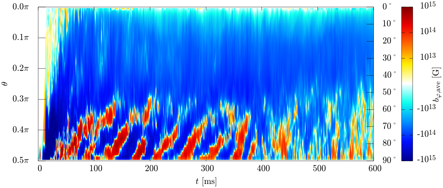
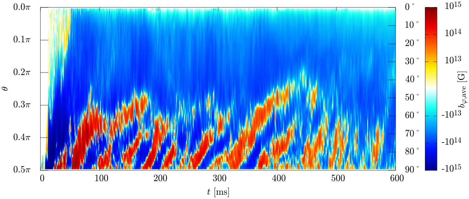
Figure 2: The profile of the average toroidal magnetic field along the polar direction ($\theta$) at $r\approx 50~{}{\rm km}$ as a function of time for models Q4B5L (top panel) and Q4B5H (bottom panel).

In the present choice of the dimensionless spin parameter for the black hole and the fairly large radius of the neutron star, the neutron star is tidally disrupted by the black hole before the binary reaches the innermost stable circular orbit both for $Q=4$ and 6. During the tidal disruption process, the neutron-star matter located in the black-hole side falls into the black hole. Specifically, $\sim 80$% of the neutron-star matter falls into the black hole in a short timescale of a few ms. On the other hand, the neutron-star matter located distant from the black hole forms a one-armed spiral structure. Due to the subsequent angular-momentum transport inside the spiral arm and the dynamical evolution of the black-hole spacetime resulting from the matter infall into it, a part of the matter in the outer part of the spiral arm gains specific energy and angular momentum. The matter which gains sufficient specific energy eventually becomes dynamical ejecta, while the other part in the spiral arm which is bound to the remnant black hole forms an accretion disk. The timescale of this stage is $\lesssim 10$ ms (see the first row of Fig. 1 for the resulting state). All these processes have been studied by a number of previous numerical-relativity work and our present result on the tidal disruption and disk formation processes is essentially the same as the previous findings.

The mass, $M_{\rm BH}$, and the dimensionless spin parameter, $\chi_{\rm BH}$, of the remnant black holes evaluated at $t=100~{}{\rm ms}$ are summarized in Table 2. Irrespective of the runs, the black-hole mass and dimensionless spin are increased by $\approx 1.05M_{\odot}$ and $\sim 0.1$, respectively, due to the matter infall. The black-hole mass is by $\sim 0.3M_{\odot}$ smaller than the initial Arnowitt-Deser-Misner (ADM) mass. The reason for this is that a part of the neutron-star matter forms an accretion disk and ejecta, and in addition, gravitational waves and neutrinos carry away the energy (see Tables 1 and 2) in the inspiral and early merger stages.

We also list the total gravitational-wave and neutrino energy emitted before $t=100$ ms, $E_{\rm GW}$ and $E_{\nu}$, and the rest mass of the matter located outside the apparent horizon at $t=100$ ms, $M_{>{\rm AH,0.1}}$, in Table 2. By comparing $M_{\rm BH}$ and $M_{\rm ADM,0}-E_{\rm GW}-E_{\nu}-M_{>{\rm AH,0.1}}$, we can assess how good (or bad) the energy conservation is satisfied in our simulation. It is found that for $Q=4$, the energy conservation is satisfied with about 0.1% and 1.1% error for high- and low-resolution runs of $Q=4$ model, and with $\ll 0.1\%$ and about 0.1% error for high- and low-resolution runs of $Q=6$ model, respectively. The reason that the accuracy depends strongly on the grid resolution for $Q=4$ (i.e., for the smaller black-hole mass) is that the accuracy for resolving the black hole depends strongly on it. This is found by taking a look at the value of the black-hole mass for $Q=4$: For the low-resolution runs, the black-hole mass is underestimated. However, the error of $\lesssim 1\%$ at $t=100$ ms is still in an acceptable level, indicating the reliability of the numerical results.

After the spiral arm winds around the black hole, a compact accretion disk is formed. The orbital period at the innermost region of the accretion disk is 1–2 ms. During the tidal disruption process, the neutron-star matter which eventually forms an accretion disk experiences a strong differential rotation stage in the spiral arm, and then, a toroidal magnetic field is developed from the initially poloidal magnetic field by winding. After the formation of the accretion disk, the winding continues to enhance the toroidal magnetic-field strength, in particular in the innermost region of the accretion disk. After the sufficient amplification of the magnetic-field strength, an outward expansion of the matter is driven toward the polar direction due to the enhanced magnetic pressure, and as a result, poloidal fields for which the strength is comparable to that of the toroidal fields are also generated. With these strong magnetic fields, the wavelength for the fastest growing mode of the MRI becomes $\sim 10$ km and can be numerically resolved (see Appendix C). Then, a turbulent state associated with the MRI is developed, and eventually, an MRI dynamo is activated in the accretion disk. This can be also observed from a spacetime diagram of the toroidal-field strength. In Fig. 2, we plot the average value of the toroidal field as a function of time and polar angle $\theta=\tan^{-1}(\sqrt{x^{2}+y^{2}}/z)$ for models Q4B5L and Q4B5H. Here, $x$, $y$, and $z$ are defined with respect to the black-hole center. The toroidal field is defined by $b_{\bar{\varphi}}=(xb_{y}-yb_{x})/\sqrt{x^{2}+y^{2}}$. The average is performed with respect to the azimuthal angle $\varphi=\tan^{-1}(y/x)$ at the selected radius of $r:=\sqrt{x^{2}+y^{2}+z^{2}}\approx 50$ km. From Fig. 2, we find the so-called butterfly structure Brandenburg and Subramanian (2005) irrespective of the grid resolution: The polarity of the toroidal magnetic field is reversed due to the turbulent motion in a periodic manner with the period of $\sim 20$ local orbital periods ($\approx 2.5$ ms). It is also found that strong magnetic-field regions move from the accretion disk to the polar region in the early stage, producing a global magnetic-field structure (see also the magnetic-field strength in the second row of Fig. 1).

During this turbulent stage, the angular momentum is transported from the inner to the outer region of the accretion disk due to the effective viscosity induced by the turbulence. In addition to this effective viscous process, magnetohydrodynamics effects such as the magneto-centrifugal effect Blandford and Payne (1982) which results from a global magnetic field could play an important role for expelling the matter from the central region. Due to these effects, the matter near the innermost stable circular orbit loses its angular momentum and falls into the black hole, while the matter in the outer part of the disk receives the angular momentum and expands gradually. As a result, the rest-mass density and the temperature in the disk decrease in the viscous timescale of order 100 ms to $1$ s (see the third to fifth rows of Fig. 1).

In addition to the disk expansion toward the equatorial direction, the matter expands toward the direction perpendicular to the orbital plane (see the entire panels of Fig. 1). Our interpretation for this expansion is that the magnetic tower effect plays a role: During the evolution of the accretion disk, the toroidal magnetic-field strength is enhanced by the MRI and winding. As a result, the magnetic pressure is enhanced to be high enough for the accretion disk to expand toward the direction perpendicular to the orbital plane (and thus the disk becomes a torus), while the serious baryon contamination in the vicinity of the rotational axis is prevented by the centrifugal force of the matter. This effect produces a funnel structure around the rotational axis (see the second to fifth rows of Fig. 1).

In spite of the enhanced magnetic-field strength, we do not find appreciable early-post-merger mass ejection (which might occur within 100–200 ms after the onset of the merger) associated with this enhancement. The absence of the clear early post-merger mass ejection agrees with some of the results found in Ref. Christie et al. (2019) in which the initial magnetic-field profile is chosen to be toroidal or weakly poloidal. Only in several previous magnetohydrodynamics studies Siegel and Metzger (2018); Fernández et al. (2019); Miller et al. (2019); Christie et al. (2019) in which a strong poloidal magnetic field is given, the early post-merger mass ejection was found. In our simulations, the magnetic-field profile in the early stage of the post-merger evolution is primarily toroidal. Thus, we consider that the early post-merger mass ejection takes place only for the case that a strong poloidal field is present in the disk at the formation of the remnant disk, although our result indicates that such strong poloidal fields are not likely to be formed soon after the merger of black hole-neutron star binaries.

Not only the magnetohydrodynamics effect but also the neutrino cooling plays an important role for the evolution of the accretion disk Fernández and Metzger (2013). In the early stage of the accretion disk, the maximum density is $\gtrsim 10^{12}\,{\rm g/cm^{3}}$ and the maximum temperature is several MeV. In addition to the high density and high temperature, the disk is massive with the mass $\gtrsim 0.1M_{\odot}$ in the early stage. In such a stage, neutrino luminosity becomes higher than $10^{53}\,{\rm erg/s}$ which is comparable to or higher than the viscous heating rate for a compact disk with a high viscous parameter Fujibayashi et al. (2020a). During the stage that the neutrino luminosity is as high as the rate of the viscous heating (and the shock heating associated with the magnetohydrodynamical activity in the present context), the matter in the accretion disk is not affected significantly by the heating effect, although the accretion disk gradually expands due to the viscous/magnetohydrodynamics angular-momentum transport and magnetic pressure resulting from the enhanced magnetic-field strength. However, with the expansion, the density and temperature of the accretion disk decrease, and consequently, the neutrino luminosity sharply decreases because the neutrino emissivity is approximately proportional to $T^{6}$ Fuller et al. (1985). As the neutrino luminosity drops below the heating rate due to the viscous and magnetohydrodynamics activities, neutrinos cannot efficiently carry away the thermal energy from the accretion disk and the thermal energy generated by the viscous/magnetohydrodynamics effect influences the evolution of the accretion disk. Specifically, convective motion of the matter at the innermost region of the disk, in which the viscous heating and shock heating are most efficient, is excited and blobs of the matter heated in the vicinity of the black hole are moved toward the outer region of the disk along the surface of the disk. As a result, the matter in the outer part of the disk obtains the thermal energy and the heated matter eventually becomes unbound from the system to be the post-merger ejecta (cf. the second and third rows of Fig. 1). This mechanism is the same as that found in the previous viscous hydrodynamics simulations Fernández and Metzger (2013); Metzger and Fernández (2014); Just et al. (2015); Fujibayashi et al. (2020a) (see also Ref. Metzger et al. (2008)). This post-merger mass ejection continues from $0.2$–0.3 s to $\sim 1$ s after the merger (i.e., after the formation of the accretion disk). We note that in addition to this convective effect, purely magnetohydrodynamical effects such as magneto-centrifugal effect Blandford and Payne (1982) could also play a role for the mass ejection.

In parallel with the accretion-disk evolution, a magnetosphere is developed in the low-density region near the rotational axis (see Fig. 1). For the merger of black hole-neutron star binaries that experience tidal disruption, such a low-density region is naturally developed because the matter is primarily ejected toward the equatorial direction. During the magnetohydrodynamics evolution of the accretion disk, a mass outflow toward the direction perpendicular to the equatorial plane is driven by the activity of the accretion disk. However, the density in the vicinity of the rotation axis is still preserved to be low because of the presence of the centrifugal force on the injected matter. Thus the accretion of the matter into the black hole proceeds primarily from the innermost region of the disk. In ideal magnetohydrodynamics, the accretion of the matter accompanies the infall of the magnetic flux into the black hole. Although the magnetic field comoving with the infalling matter falls together into the black hole, the magnetic-field line located outside the black hole can expand toward the outer direction in particular along the rotational axis which has low matter density and low gas pressure (see Sec. III.3). Such magnetic fields eventually develop a magnetosphere for which the magnetic-field lines are nearly aligned with the rotational axis (except for the vicinity of the black hole). The magnetic pressure in such a region is lower than the gas pressure of the surrounding thick torus which is formed after the activity of the accretion disk is enhanced (see the second to fifth rows of Fig. 1). In other word, the size of the magnetosphere is determined by the structure of the thick torus.

The magnetic-field lines penetrate the black hole spinning rapidly with the dimensionless spin $\gtrsim 0.8$, and thus, the system can be subject to the Blandford-Znajek mechanism Blandford and Znajek (1977) by which the rotational kinetic energy of the black hole is converted to the outgoing Poynting flux. In the presence of the matter for which the rest-mass energy density is comparable to or larger than the electromagnetic energy density, the Poynting flux cannot propagate away efficiently. However, the density in the polar region decreases with time because the matter in the vicinity of the black hole falls into the black hole and a part of the matter is expelled by the magnetic pressure. Hence, eventually, electromagnetic waves generated by the Blandford-Znajek effect can propagate away (cf. the second to fifth rows of Fig. 1). If an efficient conversion of the electromagnetic energy to the kinetic energy of the matter occurs during the subsequent propagation, a gamma-ray burst jet may be launched. Since the magnetic field has a collimated structure, the electromagnetic emission is also collimated. This collimated emission continues as far as the gas pressure of the thick and dense torus confines the magnetosphere (see Sec. III.3).

We note that the evolution processes described above are qualitatively universal irrespective of the black-hole mass, initial magnetic-field strength, and grid resolution employed in this paper. In the following subsections, we describe the quantitative details about the accretion disk evolution, mass ejection, and generation of strong Poynting flux in the magnetosphere separately.

III.2 The evolution of the accretion disk and post-merger mass ejection

III.2.1 Disk evolution and ejecta

In this subsection, we present the quantitative details on the evolution of the accretion disk and on the mass ejection. Figure 3 shows the rest mass of the matter located outside the apparent horizon $M_{>\mathrm{AH}}$ (dashed curves) and the accretion disk mass $M_{\rm disk}$ (solid curves) as functions of time. Figure 4 shows the rest mass of the unbound matter (ejecta) $M_{\mathrm{eje}}$ as a function of time. These quantities are defined by

$$M_{>{\rm AH}} := \int_{r>r_{\rm AH}}\rho_{*}d^{3}x+M_{\rm esc},$$ (4)

$$M_{\rm eje} := \int_{-hu_{t}>h_{\rm min},r>r_{\rm AH}}\rho_{*}d^{3}x+M_{\rm esc},$$ (5)

$$M_{\rm disk} := M_{>{\rm AH}}-M_{\rm eje},$$ (6)

where $\rho_{*}:=\rho\sqrt{-g}u^{t}$ with $g$ the determinant of the spacetime metric, $g_{\mu\nu}$, $u^{t}$ the time component of the four velocity, $u^{\mu}$, and $r_{\rm AH}$ denotes the coordinate radius of the apparent horizon with the respect to the black-hole puncture. $M_{\rm esc}$ denotes the rest mass escaping from the computational domain, which is calculated from

$$\dot{M}_{\rm esc} := \oint\rho\sqrt{-g}u^{i}dS_{i},$$ (7)

$$M_{\rm esc} := \int^{t}\dot{M}_{\rm esc}dt.$$ (8)

The surface integral is performed near the outer boundaries of the computational domain.

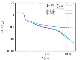
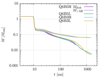
Figure 3: The time evolution of the rest mass of the matter located outside the apparent horizon (dashed curves) and the accretion-disk mass (solid curves) for all the runs with $Q=4$ (left panel) and $Q=6$ (right panel).

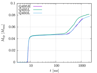
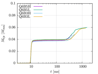
Figure 4: The time evolution of the rest mass of the unbound matter (ejecta) for all the runs with $Q=4$ (left panel) and $Q=6$ (right panel).

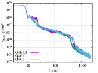
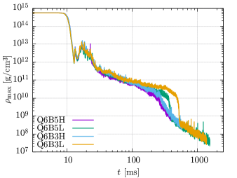
Figure 5: The time evolution of the maximum rest-mass density of the bound matter located outside the apparent horizon for all the runs with $Q=4$ (left panel) and $Q=6$ (right panel).

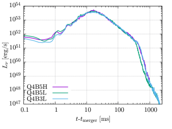
Figure 6: The time evolution of the total neutrino luminosity (sum of the luminosity for all the neutrino species) for all the runs with $Q=4$ (left panel) and $Q=6$ (right panel). The post-merger mass ejection sets in at $t-t_{\rm merger}\sim 300$–500 ms at which $L_{\nu}\sim 10^{51.5}~{}{\rm erg/s}$.

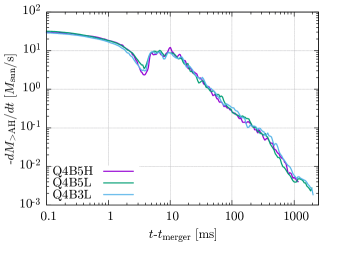
Figure 7: The time evolution of the rest-mass accretion rate calculated from $-dM_{\rm>AH}/dt$ (left panel), and the neutrino emission efficiency $L_{\nu}/(-dM_{\rm>AH}/dt)$ (right panel) for all the runs with $Q=4$.

The ejecta component is identified by considering the Bernoulli criterion; i.e., we regard the matter located outside the apparent horizon that satisfies $hu_{t}<-h_{\rm min}$ as the unbound component. Here, $u_{t}(<0)$ is the lower time component of the four velocity and $h$ is the specific enthalpy. $h_{\rm min}$ is the minimum specific enthalpy for a given electron fraction $Y_{\rm e}$ and it is obtained from the tabulated EOS employed. The value of $M_{>\mathrm{AH}}$ for $t\lesssim 20$ ms is in approximate agreement with that in our previous paper Kyutoku et al. (2018) in which magnetohydrodynamics and resulting viscous effects were absent. In the present simulation, by contrast to the one in Ref. Kyutoku et al. (2018), for $t\gtrsim$20\text{\,}\mathrm{ms}$$, $M_{>\mathrm{AH}}$ continuously decreases due to the matter accretion onto the black hole induced by the angular-momentum transport resulting from the magnetohydrodynamics effects as already mentioned in Sec. III.1. We note that the curves of $M_{>\mathrm{AH}}$ depend only weakly on the initial magnetic-field strength and grid resolution.

The value of $M_{\mathrm{eje}}$ steeply increases at two characteristic moments. The first increase is found right after the tidal disruption, and the steep increase continues only for a few ms, comparable to the dynamical timescale of the system. Thus, this mass ejection component is the dynamical ejecta. The rest mass for this component is $\approx 0.05M_{\odot}$ and $\approx 0.04M_{\odot}$ for models with $Q=4$ and 6, respectively. The result for $Q=4$ is in good agreement with our previous radiation-hydrodynamics result Kyutoku et al. (2018) because the magnetic-field strength is still weak at the tidal disruption, and hence, the magnetohydrodynamics effects play essentially no role in the dynamical mass ejection. After the steep increase, the value of $M_{\mathrm{eje}}$ remains approximately constant for the next few hundreds ms, reflecting that an efficient mass ejection activity is quiescent during this time. In this quiescent stage, however, the accretion disk is actively evolved due to the MRI and associated turbulent motion, and the density and temperature of the disk decrease (see, e.g., Fig. 5 for the rest-mass density) due to the expansion of the disk resulting from the angular-momentum transport process and enhanced magnetic pressure. As a result of the decrease in temperature, the neutrino luminosity eventually drops below the heating rate associated with the turbulent motion (cf. Fig. 6), and then, the post-merger mass ejection driven by the heating associated with the MRI turbulence sets in. Thus, the second steep increase of $M_{\mathrm{eje}}$ that starts at $t\sim 300$–$500\,{\rm ms}$ is triggered by the quick damping of the neutrino luminosity (see Fig. 6). We emphasize here that even in the presence of pure magnetohydrodynamics process (not effectively viscous process resulting from the MRI turbulence), the post-merger mass ejection appreciably occurs only after these onset time, and that, since the post-merger mass ejection continues for several hundred ms, simulations with the duration shorter than $\sim 500$ ms cannot clarify this ejection process.

The rest mass of the post-merger ejecta is $\approx 0.035M_{\odot}$ and $\approx 0.020M_{\odot}$ for models with $Q=4$ and 6, respectively, and these values are about 10% of the disk mass at its formation (at $t\sim 10$ ms). For both $Q=4$ and 6, the dynamical ejecta is the primary component of the ejecta in the present setting, and this tendency is stronger for the larger mass ratio, as discussed, e.g., in Refs. Kyutoku et al. (2015, 2021). The onset time of $t\sim 300$–$500\,{\rm ms}$ for the post-merger mass ejection depends on the initial magnetic-field strength and grid resolution by 100–200 ms. Our interpretation for this difference is that the magnetohydrodynamics turbulence is a stochastic process, and hence, the angular-momentum transport process can depend on the difference in the initial-field strength and grid resolution. However, the total ejecta mass and the properties of the post-merger ejecta do not depend strongly on them (see below for the electron fraction and velocity of the ejecta).

Figures 5 and 6 display the time evolution of the maximum rest-mass density $\rho_{\rm max}$ and the total neutrino luminosity $L_{\nu}$, respectively. For generating Fig. 6, we define the merger time $t_{\rm merger}$ as the time at which the rest-mass density reaches its local minimum value for the first time; i.e., $t\approx 10$ and 13 ms for $Q=4$ and 6, respectively. These figures indeed show that the density and neutrino luminosity steeply decrease at $t\approx 300$–500 ms. This simultaneous decrease clearly elucidates that the evolution of the accretion disk and the timing of the post-merger mass ejection are controlled by the neutrino cooling. We also note that after the onset of the post-merger mass ejection, the accretion rate of the matter onto the black hole also decreases steeply with time: see the left panel of Fig. 7.

One interesting point is that the curve of $L_{\nu}$ well reflects the evolution of the accretion disk. From $t-t_{\rm merger}\approx$1\text{\,}\mathrm{ms}$$ to $\sim 20$ ms, $L_{\nu}$ increases by orders of magnitude both for $Q=4$ and 6. This reflects the temperature increase during the formation of the accretion disk (e.g., due to the compressional heating and shock heating) and the subsequent enhancement of the turbulent state in the accretion disk due to the MRI (see, e.g., Fig. 8, which shows the increases of the electromagnetic energy in this stage). Subsequently, $L_{\nu}$ monotonically decreases for $t-t_{\rm merger}\gtrsim$20\text{\,}\mathrm{ms}$$, because in this stage, the accretion disk expands due to the angular-momentum transport process and enhanced magnetic pressure, and the density and temperature decrease gradually. However, the thermal energy generated by the heating associated with the MRI turbulence is consumed primarily by neutrino cooling prior to the onset of the post-merger mass ejection. Hence, the expansion of the accretion disk does not rapidly proceed, and thus, the mass ejection due to the thermally generated energy is suppressed. It is found that $L_{\nu}$ decreases approximately as $t^{-1.6}$ in this stage, and the decrease is fairly mild. However, after $L_{\nu}$ decreases below $\approx 10^{51.5}$ erg/s as a result of the disk expansion and resulting decrease of the temperature, the neutrino emission rate becomes smaller than the thermal energy generation rate due to the MRI turbulence. Then, the turbulent heating is used for the outward expansion of the disk efficiently, in particular through the convective motion from the inner to outer region (see footnote 1), and the post-merger mass ejection is driven. (We note that the critical neutrino luminosity, which is $\sim 10^{51.5}$ erg/s in the present case, should depend on the disk mass because the luminosity should be approximately proportional to it.) Subsequently, the neutrino luminosity exponentially drops at $t\approx 300$–500 ms irrespective of the binary mass ratio and the initial choice of the magnetic-field strength. Specifically, this post-merger mass ejection sets in when the temperature for most of the disk matter decreases below $\sim 3\,{\rm MeV}$ (cf. the top panel of Fig. 10 for a mass distribution with respect to the temperature as a function of time). This critical temperature at the onset of the post-merger mass ejection is quantitatively the same as that found in general relativistic neutrino-radiation viscous hydrodynamics simulations of black hole-torus systems Fujibayashi et al. (2020a, b). However, the time at the onset of the post-merger mass ejection is earlier than that in the viscous hydrodynamics result for the similar black-hole mass cases Fujibayashi et al. (2020b). As indicated in Refs. Christie et al. (2019); Just et al. (2015); Shibata et al. (2021), the inherent magnetohydrodynamics effects such as magento-centrifugal effect Blandford and Payne (1982) are likely to accelerate the mass ejection from the disk. The neutrino luminosity of $\approx 10^{51.5}\,{\rm erg/s}$ at the onset of the post-merger mass ejection which we find in this paper is indeed similar to that found in our recent magnetohydrodynamics study Shibata et al. (2021).

Figure 7 plots the rest-mass accretion rate onto the black hole calculated by $-dM_{>{\rm AH}}/dt$ and a neutrino emission efficiency defined by $L_{\nu}/(-dM_{>{\rm AH}}/dt)$. After the early matter infall associated with the onset of the merger, the mass accretion rate has a peak at $t-t_{\rm merger}\sim 10$ ms. This is due to the fact that the magnetic-field strength is amplified in the accretion disk and the mass accretion rate is enhanced (cf. Fig. 8). After the peak, the mass accretion rate decreases monotonically with time approximately as $\propto t^{-2}$ for $t-t_{\rm merger}\lesssim 50$ ms and as $\propto t^{-1}$ in the subsequent stage before the onset of the post-merger mass ejection. After the onset of the post-merger mass ejection, the mass accretion rate drops steeply. Broadly speaking, the curve of the neutrino emission efficiency reflects that of $L_{\nu}$. However, the peak comes at $t-t_{\rm merger}\sim 40$–50 ms, which is slightly later than the peak time of the neutrino luminosity and mass accretion rate. The reason for this is that $L_{\nu}\propto t^{-1.6}$ while $-dM_{>{\rm AH}}/dt\propto t^{-2}$ for $t-t_{\rm merger}\lesssim 50$ ms and subsequently $-dM_{>{\rm AH}}/dt\propto t^{-1}$, and thus, the peak is shifted at $t-t_{\rm merger}\sim 50$ ms. The maximum neutrino emission efficiency is $\sim 8$%–10%. Keeping the difference in the disk mass in mind, this value agrees broadly with those found in our viscous hydrodynamics simulations for similar black-hole mass ($M_{\rm BH}=6M_{\odot}$) and dimensionless spin ($\chi_{\rm BH}=0.8$) Fujibayashi et al. (2020b).

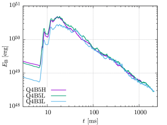
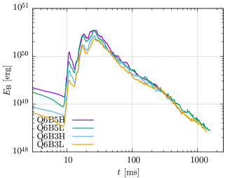
Figure 8: The time evolution of the electromagnetic energy evaluated for the outside of the apparent horizon for all the runs with $Q=4$ (left panel) and $Q=6$ (right panel)

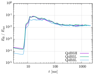
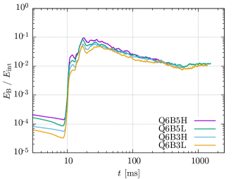
Figure 9: The time evolution of the ratio of the electromagnetic energy to the internal energy evaluated for the outside of the apparent horizon for all the runs with $Q=4$ (left panel) and $Q=6$ (right panel).

III.2.2 Magnetic-field evolution

Figures 8 and 9 show the time evolution of the electromagnetic energy, $E_{\rm B}$, and the ratio of the electromagnetic energy to the internal energy, $E_{\rm int}$, respectively. Here, $E_{\rm B}$ and $E_{\rm int}$ are defined, respectively, by

$$E_{\rm B} := \frac{1}{8\pi}\int_{r>r_{\rm AH}}u^{t}\sqrt{-g}\,b_{\mu}b^{\mu}d^{3}x,$$ (9)

$$E_{\rm int} := \int_{r>r_{\rm AH}}\rho_{*}\varepsilon d^{3}x,$$ (10)

and $\varepsilon$ denotes the specific internal energy. Here we note that the energy-momentum tensor in the ideal magnetohydrodynamics is written as

$$T_{\mu\nu} = \rho hu_{\mu}u_{\nu}+Pg_{\mu\nu}$$ (11)

$$+ {1\over 4\pi}\left(b^{\alpha}b_{\alpha}u_{\mu}u_{\nu}+{1\over 2}b^{\alpha}b_{\alpha}g_{\mu\nu}-b_{\mu}b_{\nu}\right),$$

and with $h=c^{2}+\varepsilon+P/\rho$, we have

$$u^{t}\sqrt{-g}T_{\mu\nu}u^{\mu}u^{\nu}=\rho_{*}(c^{2}+\varepsilon)+{1\over 8\pi}u^{t}\sqrt{-g}\,b^{\mu}b_{\mu}.$$ (12)

Here we recover $c$ to clarify the physical units. Thus, the choice of $E_{\rm int}$ and $E_{\rm B}$ stems from Eq. (12).

During the merger stage, the magnetic-field strength in the accretion disk is amplified quickly in a short timescale of a few ms. This is initially induced by the magnetic winding associated with the differential rotation in the accretion disk. In the Keplerian disk with the presence of the poloidal magnetic field of the cylindrically radial component $B^{\varpi}$, the strength of the toriodal magnetic field $B^{T}$ increases approximately linearly with time until a saturation as (e.g., Ref. Shibata et al. (2006))

$$B^{T}\approx{3\over 2}B^{\varpi}\Omega t,$$ (13)

where $\Omega$ denotes the local angular velocity. For a black hole with the dimensionless spin of $0.8$, the angular velocity at the innermost stable circular orbit of the black hole is $\Omega_{\rm ISCO}\approx 0.174M_{\rm BH}^{-1}\approx 5.43\times 10^{3}(M_{\rm BH}/6.5M_{\odot})^{-1}$ rad/s Bardeen et al. (1972). Thus for the models of $Q=4$ and $Q=6$, the matter near the innermost stable circular orbit rotates with the orbital period of $\approx 1.2$ and 1.6 ms, respectively. This implies that in the first $\sim 10$ ms, the toroidal field strength can be $\sim 60$–80 times of $B^{\varpi}$, the maximum of which is $\sim 10^{14}$ G at the formation of the accretion disk (i.e., much weaker than the field strength in the neutron star initially given) in the present simulations. This is the reason that the initial steep amplification to $E_{\rm B}>10^{50}$ erg is found in our present simulations. Because the winding timescale is quite short, the magnetic-field amplification by $\sim 3$ orders of magnitude in $\lesssim 100$ ms is possible even in the absence of other instabilities such as MRI: Even for the initial value of $B^{\varpi}=10^{12}$ G, the toroidal field can be amplified to $\sim 10^{15}$ G in $\sim 100$ ms. After the sufficient amplification of the toroidal magnetic field, an outward expansion of the accretion disk is driven toward the polar direction due to the enhanced magnetic pressure and a poloidal field with its strength comparable to that of the toroidal field is also generated. We note that the Kelvin-Helmholtz instability that takes place during the winding of the spiral arm around the black hole and collision between different parts of the spiral arm may also contribute partly to the magnetic-field amplification.

After the initial amplification of the magnetic-field strength, the ratio of $E_{\rm B}/E_{\rm int}$ reaches $\sim 0.05$–0.1. Then, the magnetic-field growth is saturated. The electromagnetic energy at the saturation, $E_{\rm B,sat}$, is smaller for the smaller value of the initial magnetic-field strength. However, the relative difference in the saturated electromagnetic energy between models with different initial magnetic-field strengths is not as large as that in the initial electromagnetic energy. Furthermore, the electromagnetic energy for $t\gtrsim 30$ ms depends only weakly on the initial condition (as well as on the grid resolution). Thus, we infer that the amplification and saturation of the magnetic-field strength take place in a universal manner irrespective of the initial magnetic-field strength.

When reaching the saturation, the typical magnetic-field strength is $10^{15}$ G (cf. Fig. 2) and the maximum rest-mass density is $\sim 10^{11}$–$10^{12}~{}{\rm g/cm^{3}}$ in the innermost region. Thus the Alfvén velocity is $\approx b/\sqrt{4\pi\rho}\approx 9\times 10^{8}$ cm/s$\,(b/10^{15}\,{\rm G})(\rho/10^{11}\,{\rm g\,cm^{-3}})^{-1/2}$ and the wavelength of the fastest growing mode of the MRI is typically $\sim 10$ km Balbus and Hawley (1998). As a result, the wavelength of this unstable mode is covered by tens of grid points in our setting (see Appendix C), and hence, the effect of the MRI comes into play subsequently. With the evolution of the disk, the typical magnetic-field strength and rest-mass density decrease, but in the equipartition stage (see below), the Alfvén velocity is always of order $\sqrt{E_{\rm B}/E_{\rm int}}(\sim 10\%)$ of the sound speed, which changes weakly with time. Thus, the wavelength of the fastest growing mode of the MRI is always covered by tens of grid points in the present setting. Indeed, our numerical analysis shows that the wavelength is covered by $\sim 10$ grid points for the region with $\rho=10^{11}\,{\rm g/cm^{3}}$, and more (several tens of) grid points for lower density region.

After the MRI starts playing a role, a turbulent state is developed in the accretion disk and an effective viscosity is induced. We evaluate the following ratio of the anisotropic stress to the pressure

$${\color[rgb]{0,0,0}\alpha_{ij}:=\left\langle\left|{1\over P}\left(\rho h\hat{u}_{i}\hat{u}_{j}-{1\over 4\pi}b_{i}b_{j}\right)\right|\right\rangle_{\rm ave},}$$ (14)

where $i\not=j$ ($i$, $j=x,y,z$) and $\langle\cdots\rangle_{\rm ave}$ denotes the spatial average with the weight of the rest-mass density ($\rho_{*}$) for the region with $z\geq 0$ and $\rho\geq 10^{7}\,{\rm g/cm^{3}}$. $\hat{u}_{i}$ is defined by $u_{i}-\langle u_{i}\rangle_{t,{\rm ave}}$ where $\langle u_{i}\rangle_{t,{\rm ave}}$ denotes the local time average of $u_{i}$. The time average needs to be subtracted from $u_{i}$ to eliminate the contribution of coherent motion (not random motion) for evaluating the anisotropic stress associated with the turbulent motion. We find that all the components of $\alpha_{ij}$ are between $\approx 0.02$ and $0.1$ at the onset of the post-merger mass ejection depending only weakly on the initial magnetic-field strength and grid resolution. The values of $\alpha_{ij}$ are comparable to the viscous alpha parameter often employed in the viscous hydrodynamics simulations (e.g., Refs. Fernández et al. (2019); Fujibayashi et al. (2020a, b)). The value is slightly larger than the result of previous magnetohydrodynamics simulations of black-hole accretion disks De and Siegel (2021) but this difference is likely to come from the difference in the definition of $\alpha_{ij}$. In this stage, the ratio of $E_{\rm B}/E_{\rm int}$ is preserved to be of $O(10^{-2})$.

As a result of the viscous angular-momentum transport, the matter in the inner region of the accretion disk falls into the black hole while the matter in the outer part expands outward. Because of the matter infall into the black hole, the rest mass of the accretion disk decreases (see Fig. 3), and associated with the decrease in the rest mass, the electromagnetic energy decreases with time although the ratio of $E_{\rm B}/E_{\rm int}=O(10^{-2})$ is preserved. Thus, for $t\gtrsim 100$ ms, the accretion disk is in a quasi-steady equipartition state; the magnetic-field energy relaxes to $\sim 1\%$ of the internal energy irrespective of the mass and internal energy of the accretion disk. It is interesting to point out that the electromagnetic energy decreases approximately in proportion to $t^{-1}$. All these features are found both for the models of $Q=4$ and $Q=6$ irrespective of the initial magnetic-field strength and grid resolution.

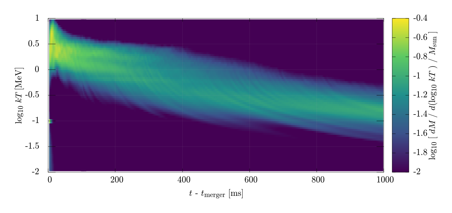
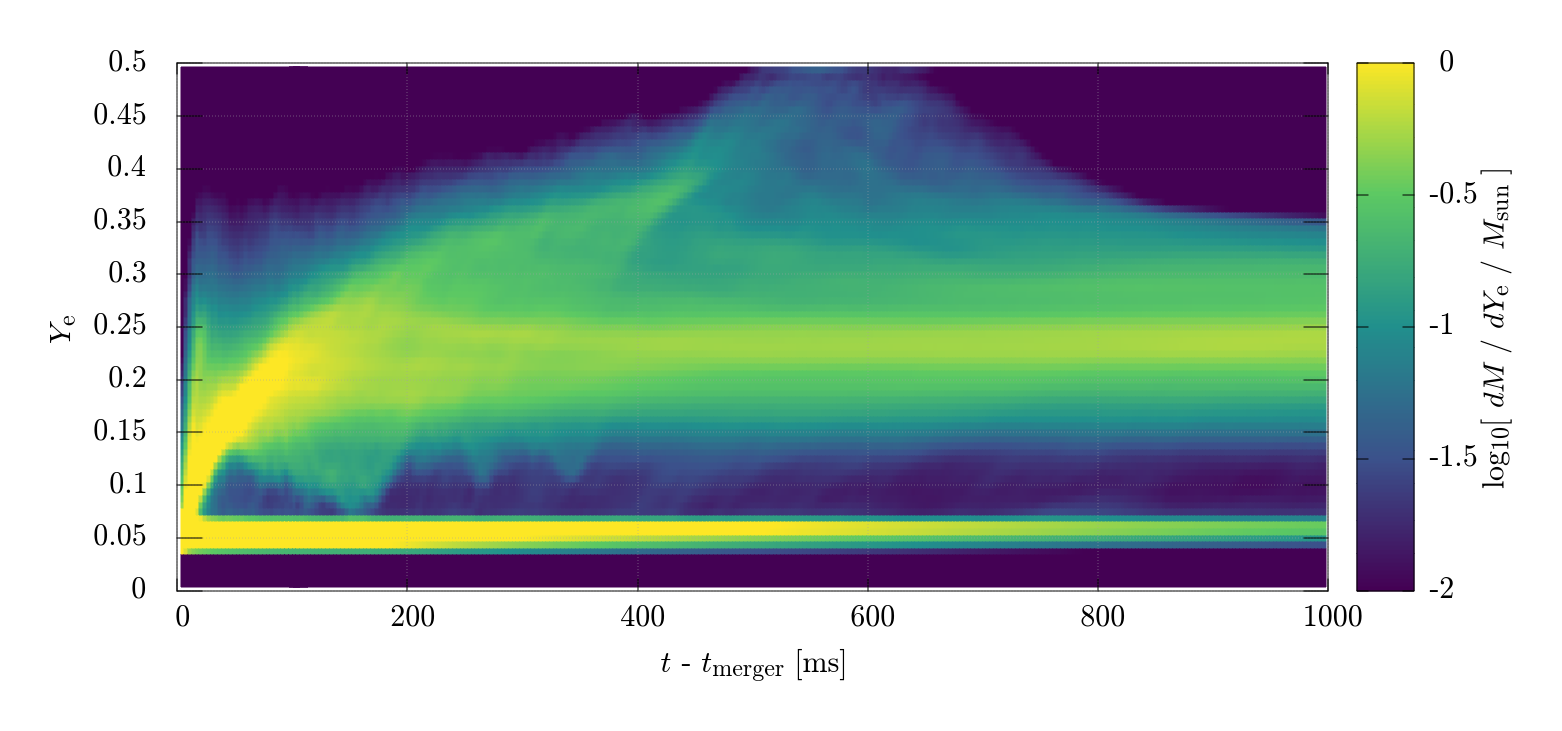
Figure 10: Time evolution of the mass histograms with respect to the temperature (upper panel) and electron fraction (lower panel) for model Q4B5H. The post-merger mass ejection sets in when the temperature for most of the matter decreases below $3~{}{\rm MeV}$ at $t\sim 400$ ms for this model. Note that the matter only in the computational domain is taken into account for plotting this figure, and thus, the matter which has escaped from the computational domain is neglected in the late stages. Thus, for $t\gtrsim 300~{}{\rm ms}$, the dynamical ejecta mass decreases with time.

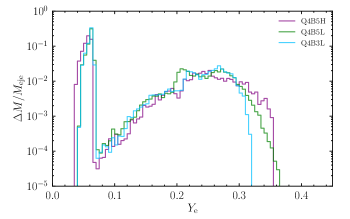
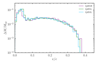
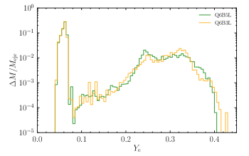
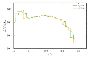
Figure 11: Mass histogram as functions of the electron fraction (left panels) and the velocity (right panels) of ejecta for the models with the simulation duration longer than $1\,{\rm s}$ (models Q4B5H, Q4B5L, Q4B3L, Q6B5L, and Q6B3L). Models with $Q=4$ and $Q=6$ are displayed in the upper and lower panels, respectively.

III.2.3 Property of ejecta

Now we turn our attention to the properties of the ejecta. The bottom panel of Fig. 10 displays the mass distribution of the remnant matter with respect to the electron fraction $Y_{\rm e}$ for model Q4B5H. This shows that there are two characteristic peaks of $Y_{\rm e}$ at the regions around 0.05 and of 0.25–0.35, respectively. The former peak is associated primarily with the dynamical ejecta and the latter is with the accretion disk for $t\lesssim 400$ ms and post-merger ejecta for $t\gtrsim 400$ ms. This figure clearly shows that the dynamical ejecta component with $Y_{\rm e}=0.03$–0.07 comes directly from the neutron star, because the values are unchanged from the beginning. That is, this dynamical ejecta component is not essentially affected by thermal or weak-interaction processes in the merger and post-merger stages.

By contrast, the electron fraction of the post-merger ejecta is found to be determined by the evolution process of the accretion disk, in which the typical electron fraction increases from $\sim 0.05$ to $\sim 0.25$ for $0<t\lesssim 200$ ms. As already mentioned, in this stage, the accretion disk gradually expands due to the viscous and magnetohydrodynamical angular-momentum transport and magnetic pressure by the amplified magnetic-field strength, and its rest-mass density and temperature monotonically decrease. In the disk with its optical depth to neutrinos $\lesssim 1$, the electron fraction is determined predominantly by the reaction equilibrium between electron/positron capture reactions if the temperature is high enough (typically $kT\gtrsim 2$–3 MeV; see Refs. Beloborodov (2003); Fujibayashi et al. (2020b); Just et al. (2022)) for their timescale to be shorter than that of the disk expansion. Due to the disk expansion, the electron degeneracy becomes weak, and as a result, the electron fraction is shifted to higher values in the reaction equilibrium state. With the decrease of the temperature, the neutrino luminosity decreases approximately in proportion to $T^{6}$. As already mentioned, the post-merger mass ejection sets in when the neutrino luminosity drops below $\sim 10^{51.5}\,{\rm erg/s}$, which occurs for $t\gtrsim 300$ ms. The typical value of $Y_{\rm e}$ for the post-merger ejecta is determined around this timing, resulting in $Y_{\rm e}\approx 0.25\pm 0.10$.

Figure 11 displays the rest-mass histogram as functions of the electron fraction and velocity for the ejecta component for the models for which the simulation duration is longer than 1 s. The mass histogram is derived for the ejecta component outgoing from the radius of $\approx 10^{4}$ km. As described in the previous paragraphs, there are two distinct $Y_{\rm e}$ components for the ejecta, and this feature is clearly observed in Fig. 11. The dynamical ejecta component always has $Y_{\rm e}\approx 0.03$–0.07 irrespective of the black-hole mass. By contrast, the distribution of $Y_{\rm e}$ for the post-merger ejecta component depends on the black-hole mass in the present results. Specifically, for larger black-hole mass, the value of $Y_{\rm e}$ tends to be larger. As a result, the peak of $Y_{\rm e}$ changes from $\sim 0.25$ for $Q=4$ to $\sim 0.31$ for $Q=6$. This is in agreement with our finding in our viscous hydrodynamics studies Fujibayashi et al. (2020b) (see also Refs. Fernández et al. (2020); Just et al. (2022)), and the reason is as follows: In the condition that the disk mass has an approximately identical value, the density of the disk can be higher for the lower black-hole mass (the lower mass ratio, $Q$, in the present context), because the tidally disrupted matter can have a more compact orbit around the black hole due to the smaller radius of its innermost stable circular orbit. Associated with this effect, the temperature is enhanced due to the compression and stronger shock heating, resulting in the higher neutrino emissivity and reducing the entropy per baryon of the matter in the accretion disk (cf. Fig. 6). With the lower entropy per baryon, the degree of the electron degeneracy becomes higher and the neutron-richness is enhanced. Therefore, for the lower black-hole mass, the electron fraction of the post-merger ejecta becomes slightly lower. Figure 11 shows that this effect is found irrespective of the initial-magnetic field strength and grid resolution (thus it is physical).

The right panels of Fig. 11 present the rest-mass histogram as a function of the ejecta velocity. Again, there are two components. Here, the low-velocity component with $v/c\lesssim 0.08$ stems primarily from the post-merger ejecta, while the high-velocity component stems from the dynamical ejecta. We note that the velocity distribution for the dynamical ejecta is in good agreement with that in our previous study Kyutoku et al. (2018), and the typical velocity of the post-merger ejecta agrees approximately with that found in viscous hydrodynamics simulations (e.g., Refs. Fujibayashi et al. (2020a, b)). As we reported in Ref. Kyutoku et al. (2015), the velocity of the dynamical ejecta is at highest $\sim 0.4c$. This is in contrast to the case of binary neutron star mergers in which the maximum ejecta velocity can be $\gtrsim 0.8c$ Hotokezaka et al. (2013).

Our present results confirm that there are two distinct ejecta components, low-$Y_{\rm e}$ and high-velocity component, and relatively-high-$Y_{\rm e}$ and low-velocity component, as many previous numerical work have suggested. By our self-consistent simulations, the distinction of two components emerges clearly. The former (dynamical ejecta) is likely to synthesize heavy $r$-process elements, while the latter (post-merger ejecta) is likely to synthesize relatively light $r$-process elements as well as heavy ones (e.g., Refs. Wanajo et al. (2014); Just et al. (2015)). Then, the former component is likely to shine as a red kilonova while the latter one is likely to contribute to a blue-kilonova component Metzger and Fernández (2014). However, the detailed light curve and spectrum are determined by a non-trivial radiation transfer effect Kawaguchi et al. (2020). It is also likely that the light curve depends on the mass ratio $Q$. Thus, a nucleosynthesis calculation and radiation transfer simulation are topics to be explored as follow-up work.

III.3 Magnetic field in the funnel region and the relation to short gamma-ray bursts

In addition to aforementioned ejected matter (dynamical and post-merger ejecta), we find a launch of an outflow of the matter and Poynting flux in the narrow funnel region established near the rotational axis of the black hole (see Fig. 12). In particular, the isotropic Poynting luminosity estimated for most of the runs is comparable to the typical luminosity of short-hard gamma-ray bursts Nakar (2007); Berger (2014). In this section, we discuss the quantitative details on this result.

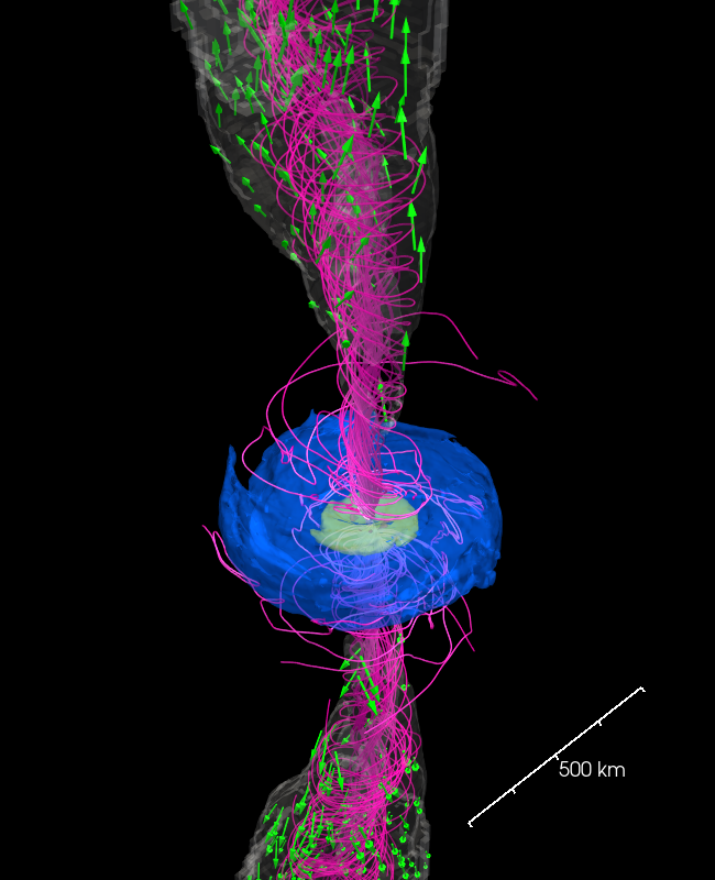
Figure 12: Snapshots of the rest-mass density profile (blue and green contours) with the magnetic-field lines (pink curves), unbound matter (white color) and its velocity (green arrow) for model Q4B5L at $t=300$ ms. Magnetic-field lines penetrating the black-hole horizon are displayed. See also the following link for the time evolution: https://www2.yukawa.kyoto-u.ac.jp/~kota.hayashi/Q4B5L-3D.mp4

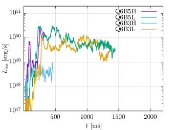
Figure 13: $L_{\rm iso}$ as a function of time for all the runs with $Q=4$ (left panel) and $6$ (right panel). The Poynting luminosity is evaluated at $r\approx 1500~{}{\rm km}$ for all the runs.

Irrespective of the black-hole mass, initial magnetic-field strength, and grid resolution, tidal disruption of the neutron star takes place in our present setting and a magnetized accretion disk is formed around the central black hole. As already mentioned in the previous subsections, the magnetic-field strength in the accretion disk is increased by the winding and MRI, and then, a turbulent state is established at $\sim 30$–40 ms after the tidal disruption. Subsequently, the accretion disk evolves primarily due to the viscous effect stemming from the MRI turbulence. As already mentioned in the previous subsection, the magnetic-field strength is determined by an equipartition state, i.e., by the internal energy of the matter, which is typically $\rho c_{\rm s}^{2}$ where $c_{\rm s}$ is the sound speed of order $10^{9}$ cm/s in the dense region of the disk. Since $E_{\rm B}/E_{\rm int}$ is of $O(10^{-2})$, the magnetic-field strength can be approximated as $\sim 0.1\sqrt{8\pi\rho c_{\rm s}^{2}}\sim 5\times 10^{14}(\rho/10^{12}\,{\rm g\,cm^{-3}})^{1/2}(c_{\rm s}/10^{9}\,{\rm cm\,s^{-1}})$ G near the inner edge of the accretion disk. The order of this field strength is indeed found in the accretion disk (see, e.g., Fig. 2). By the angular-momentum transport, the matter in the innermost part of the accretion disk falls continuously into the black hole, and in this infall, the magnetic fluxes also fall in. As a result, the poloidal magnetic-field lines for which the field strength is $\gtrsim 10^{14}$ G at the horizon penetrate the black hole. Here, the infall magnetic fluxes do not have aligned polarity because the accretion process is determined by the turbulence in the accretion disk, and hence, the magnetic-field strength on the horizon does not monotonically increase. On the other hand, the poloidal magnetic fields in the polar region are twisted by the black-hole spin, and hence, the field strength could be larger than that for the accretion disk in the presence of a rapidly spinning black hole. Due to the twisting associated with the black-hole spin, the toroidal magnetic-field strength dominates over the poloidal one in the vicinity of the black hole (cf. Fig. 12).

However, such amplified magnetic fields do not immediately form a global magnetosphere. The reason for this is that at tidal disruption, a dense atmosphere ($\rho\sim 10^{7}~{}{\rm g/cm^{3}}$) is formed in the polar region by the matter expelled by shocks generated during the winding and shock heating in the spiral arm. The matter also comes from the accretion disk due to its turbulent activity. Although a part of the matter in the polar region near the black hole eventually falls into the black hole, a certain fraction of the matter has to be expelled by the magnetic force to form a low-density magnetosphere. For this, the toroidal magnetic field amplified by the twisting due to the black-hole spin plays an important role, because a tower-like outflow is driven from the neighborhood of the black hole by this magnetic effect Ruiz et al. (2018). Hence, eventually, the matter energy density decreases below the magnetic energy density of $b^{2}/8\pi$ in the polar region of the black hole. This is satisfied for $\rho<b^{2}/8\pi c^{2}=4.4\times 10^{5}(b/10^{14}\,{\rm G})^{2}\,{\rm g/cm^{3}}$. Then, the magnetic pressure pushes the matter toward the outward direction along the rotation axis, establishing a low-density region near the rotational axis. During this process, the magnetic-field lines also expand outwardly, and a large-scale magnetosphere near the rotational axis is formed. In this region, the poloidal field is dominant (see Fig. 12). As a result, the rest-mass density decreases in the black-hole polar region, leading to the formation of the so-called funnel structure. At the funnel wall, the magnetic pressure is lower than the gas pressure of the surrounding thick torus and envelope, and hence, the magnetosphere is sustained by the surrounding matter.

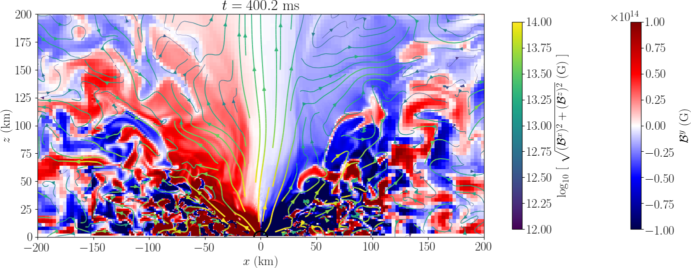
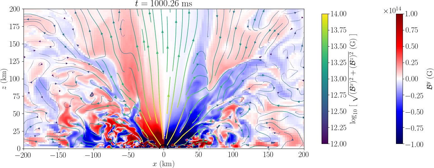
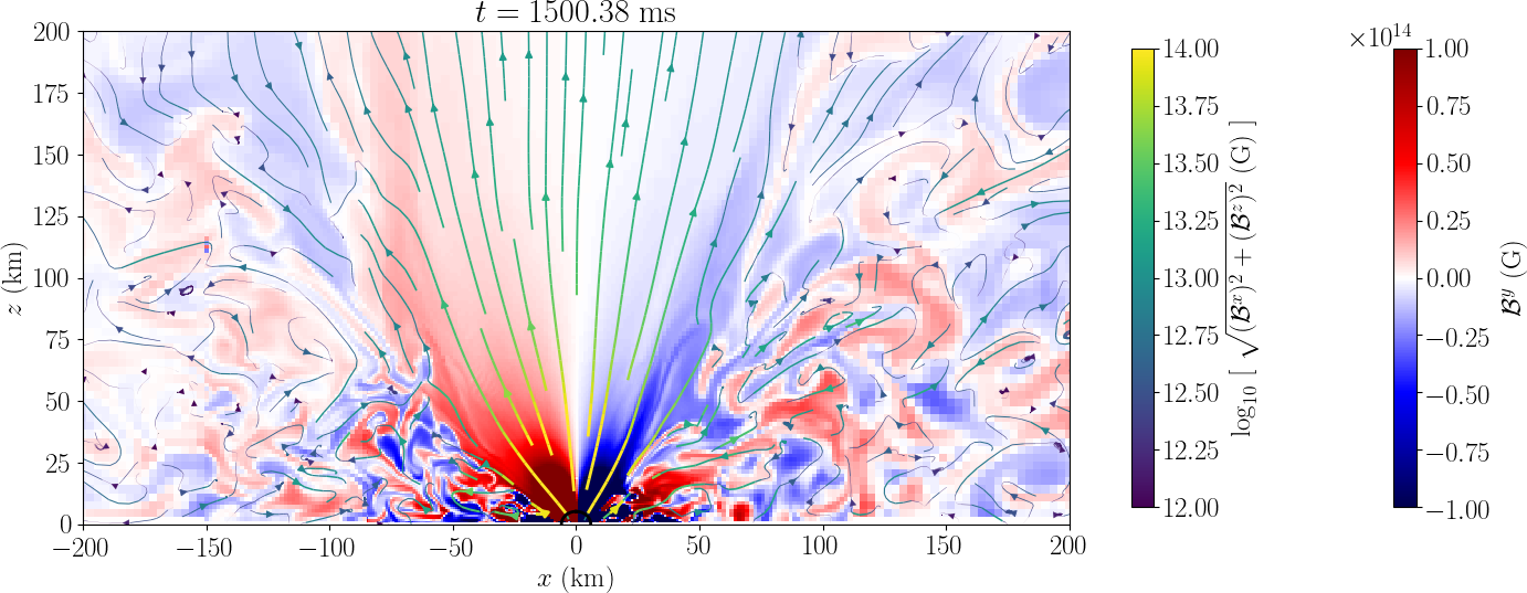
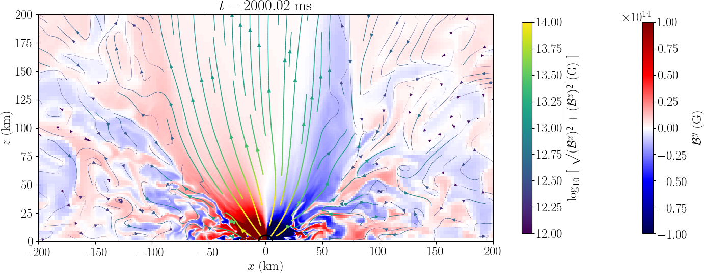
Figure 14: The snapshot of the toroidal magnetic field (color profile) together with the poloidal magnetic-field lines (curves) on the $x$-$z$ plane at selected time slices for model Q4B5L. See also the following link for an animation: https://www2.yukawa.kyoto-u.ac.jp/~kota.hayashi/Q4B5L-mf.mp4

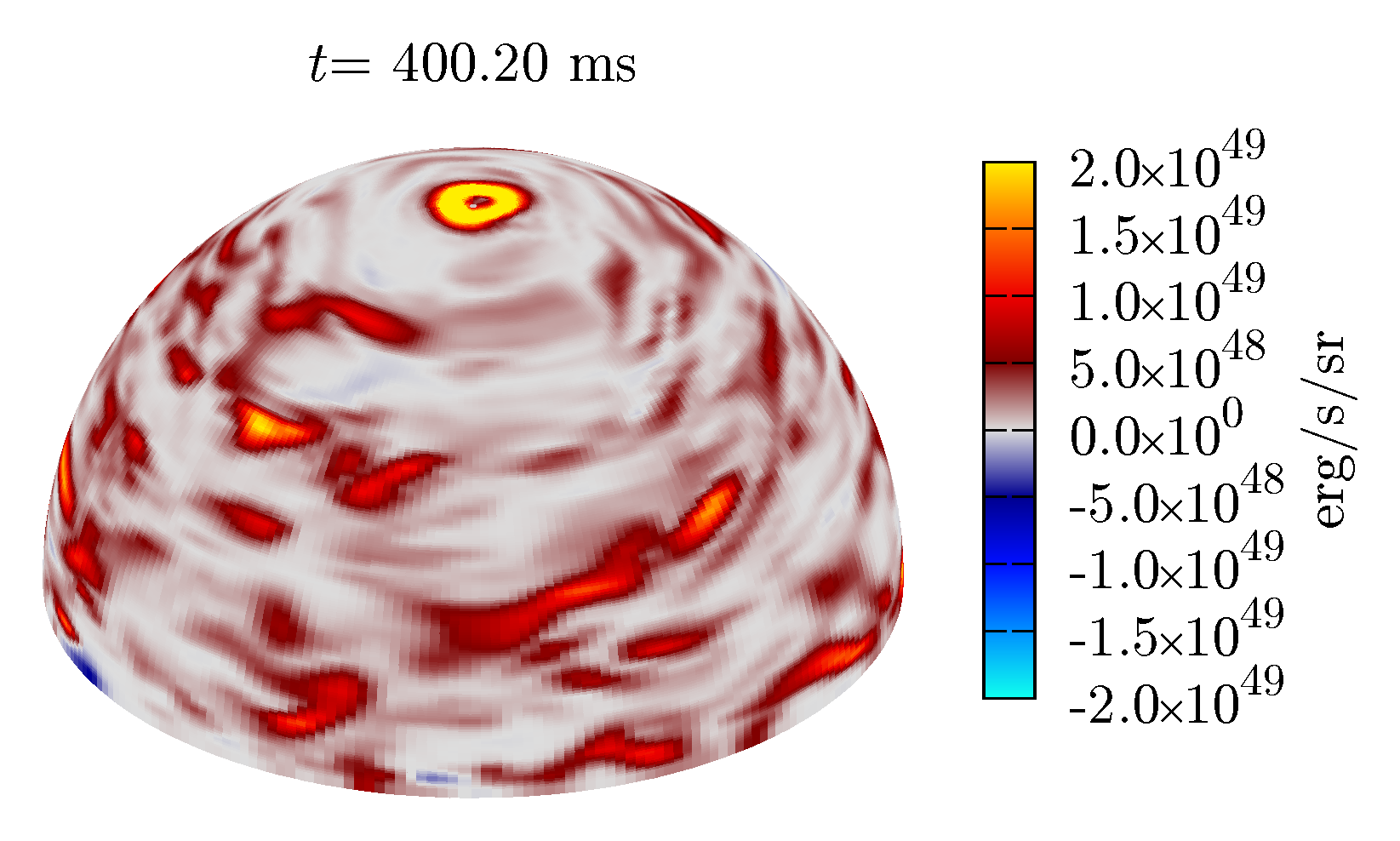
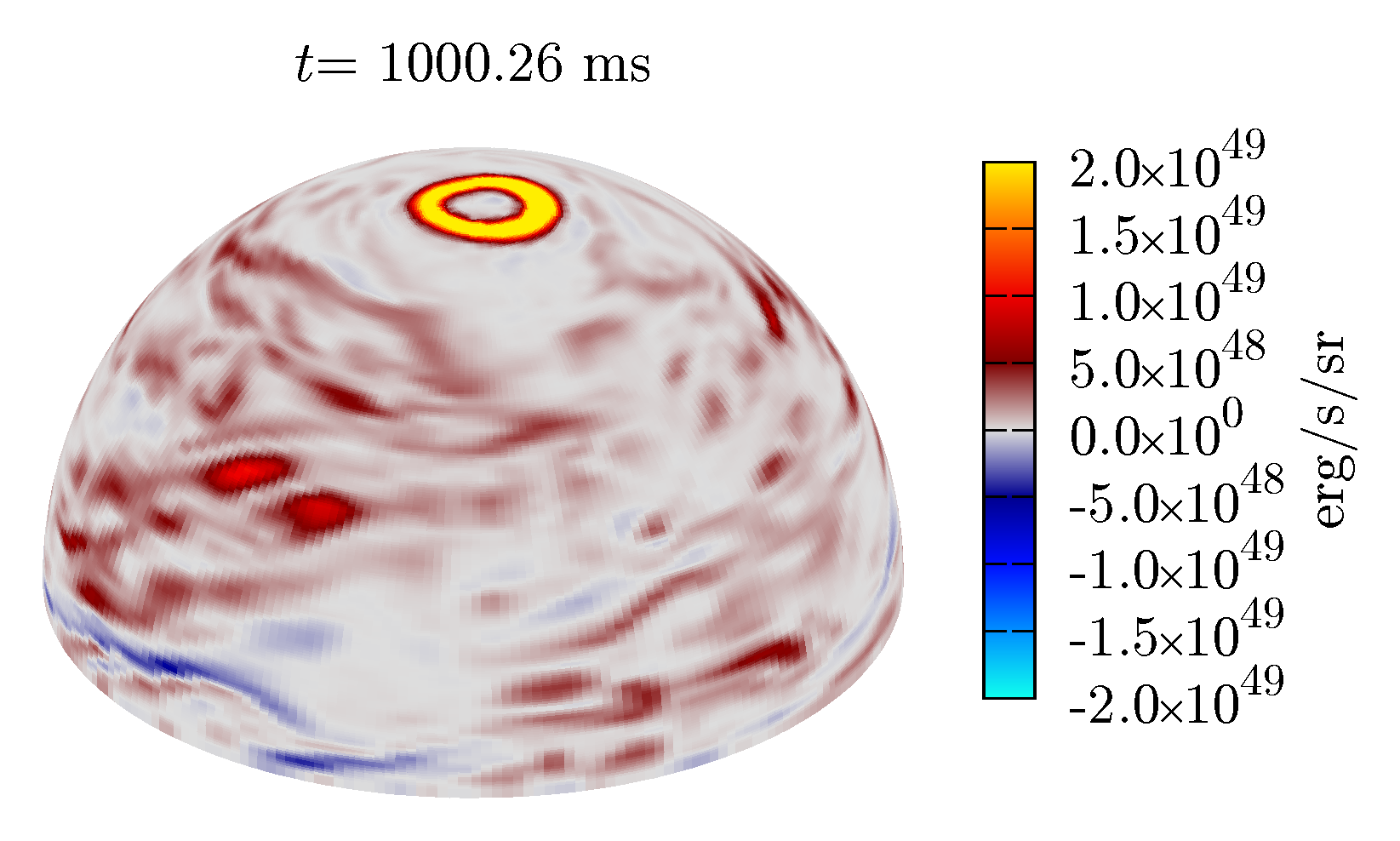
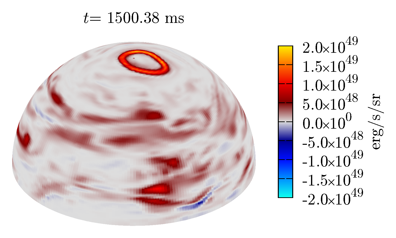
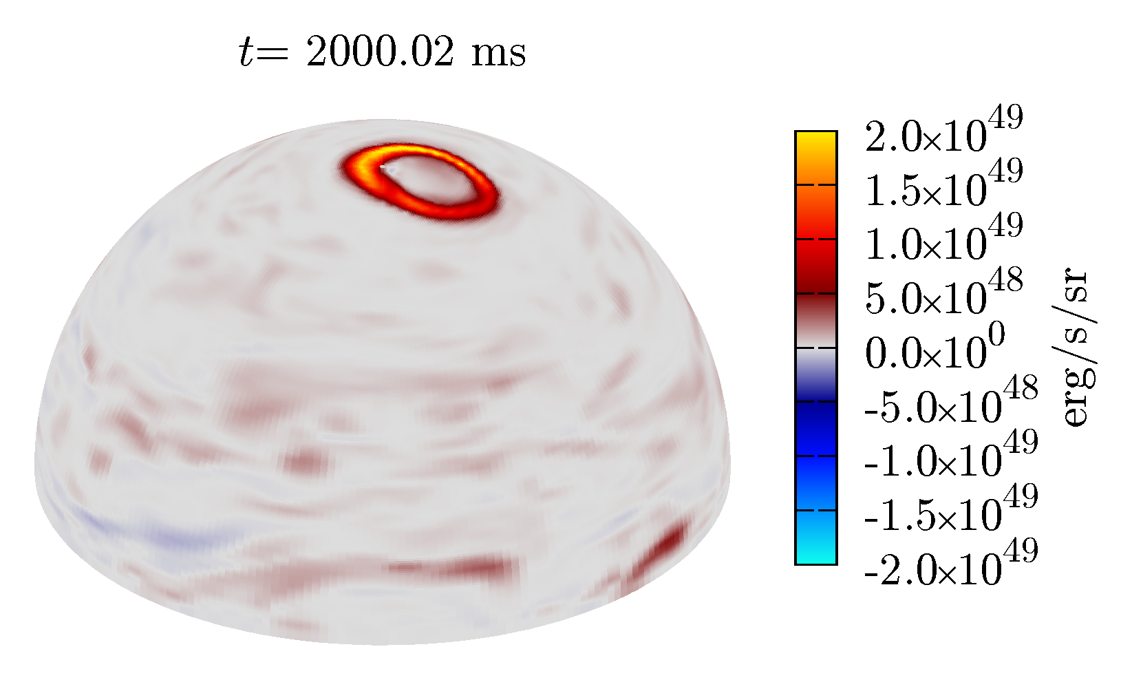
Figure 15: The angular distribution of the Poynting flux per steradian on a sphere of $r\approx 1500$ km for model Q4B5L at selected time slices. The bright color displayed in the polar region stems from the Blandford-Znajek effect, while for other regions, the magnetic fields accompanying with the outflowing matter contribute mainly to the Poynting flux. The opening angle of the Poynting flux in the polar region is shown to increase with time. See the following link for an animation: https://www2.yukawa.kyoto-u.ac.jp/~kota.hayashi/Q4B5L-f3D.mp4

Inside the funnel wall, the electromagnetic energy dominates over the rest-mass energy, and thus, an approximately force-free magnetosphere is formed. Here, the typical ratio of the electromagnetic energy density to the rest-mass energy density is 10–100. In such a region, the rotational kinetic energy of the black hole is extracted by the Blandford-Znajek mechanism Blandford and Znajek (1977) and transformed into the Poynting flux which propagates outward (see Appendix D for the result that shows the presence of the outgoing energy flux from the black hole). Figure 13 shows the time evolution of $L_{\rm iso}$: an isotropic Poynting luminosity, which we define using the Poynting luminosity for $\theta<10^{\circ}$ and $r\approx 1500\,{\rm km}$ as

$$L_{\rm iso}:=\frac{2}{1-\cos(10^{\circ})}L_{\theta<10^{\circ},r\approx 1500\,{\rm km}},$$ (15)

where

$$L_{\theta<10^{\circ},r\approx 1500\,{\rm km}}:=-\int_{\theta<10^{\circ},r\approx 1500\,{\rm km}}{T^{{\color[rgb]{0,0,0}\mathrm{(EM)}}}}^{~{}r}_{t}\sqrt{-g}dS_{r}.~{}~{}$$

$T^{\mathrm{(EM)}}_{~{}\mu\nu}$ denotes the electromagnetic part of the energy-momentum tensor. We here choose a particular value ($10^{\circ}$) for the surface integral because the opening angle of the funnel region is initially as narrow as $\sim 10^{\circ}$ (see Figs. 14 and 15).

Figure 13 shows that the typical maximum value of $L_{\rm iso}$ is of order $10^{50}\,{\rm erg/s}$ and $L_{\rm iso}$ varies with time irrespective of the black-hole mass and initial magnetic-field strength. This varying isotropic luminosity together with the opening angle of $\theta\sim 10^{\circ}$ (cf. Fig. 15) is in a fair agreement with those for short-hard gamma-ray bursts in the assumption that the conversion efficiency of the Poynting flux to the gamma-ray radiation is sufficiently high (i.e., close to unity) Nakar (2007); Berger (2014).

The stage with a high value of $L_{\rm iso}\gtrsim 10^{50}$ erg/s continues broadly for 1 s. Subsequently, the isotropic luminosity starts decreasing. This is due to the fact that the opening angle of the funnel region increases and the magnetic-flux density is reduced. Remember that the funnel region is determined by the gas pressure of the thick torus at the funnel wall. In the long-term evolution of the accretion torus, the rest-mass density and associated gas pressure around the funnel wall decrease with time due to the post-merger mass ejection. On the other hand, the total magnetic flux penetrating the black hole does not significantly decrease in the ideal magnetohydrodynamics, and thus, the decrease in the magnetic pressure is not as significant as the gas pressure at the funnel wall. As the rest-mass density decreases, thus, the magnetic pressure exceeds the gas pressure at the original position of the funnel wall, and as a result, the funnel wall expands gradually.

Figure 14 displays the snapshot of the toroidal magnetic field together with the poloidal magnetic-field lines on the $x$-$z$ plane at selected time slices. This indeed shows that the configuration of the magnetic-field lines changes from an aligned collimated one near the rotational axis to a more spread one for late time with $t\gtrsim 1$ s.

Since the collimation of the poloidal magnetic-field lines is loosened, the Poynting flux in the vicinity of the rotational axis also decreases gradually. Figure 15 shows that the opening angle of the strong Poynting-flux ($-{T^{{\color[rgb]{0,0,0}\mathrm{(EM)}}}}^{~{}r}_{t}\sqrt{-g}$) region increases from $\lesssim 10^{\circ}$ to $\sim 20^{\circ}$ and the intensity of the Poynting flux becomes weak with time. The reason that the peak of the Poynting flux is located near the funnel wall is that the magnetic-field lines near the funnel wall penetrate the equatorial regions of the spinning black hole, and hence, the Blandford-Znajek effect can be more efficient. If the Poynting flux indeed determines the luminosity of short-hard gamma-ray bursts, its brightness also should decrease for $t\gtrsim 1$ s. This mechanism could be interpreted as a reason that the timescales of short-hard gamma-ray bursts are less than 2 s with the typical timescale of $\sim 1$ s. Specifically, our numerical results propose that the timescale of $\sim 1$ s is determined by the evolution timescale of the accretion disk (torus), which is determined by the neutrino cooling and magnetohydrodynamics turbulence (effectively viscous process) that control the post-merger mass ejection.

A word of the caution is appropriate here. First, the turbulence and dynamo activated by the MRI in the accretion disk are stochastic processes. This implies that the poloidal magnetic-field flux penetrating the black hole could not be precisely predicted. For example, by the accretion of the magnetic fields with a random polarity, the magnetic flux that penetrates the black hole may be smaller than that in the accretion disk. Hence, it is reasonable that the magnetic-field strength could not be always as strong as the one necessary for explaining typical short-hard gamma-ray bursts. Indeed, for model Q6B3H, the Poynting luminosity is by one order of magnitude lower than those for other models. In this case, the magnetic-field strength on the black-hole horizon is about 1/3 of those for other models. Therefore, broadly speaking, there are two possible cases: (1) A magnetosphere with strong poloidal magnetic fields is formed near the rotational axis of a spinning black hole. In this case, the maximum isotropic Poynting luminosity of $10^{50}$–$10^{51}~{}{\rm erg/s}$ consistent with typical short-hard gamma-ray bursts can be generated; (2) Due to the stochastic process of the MRI-induced turbulent motion, poloidal magnetic fluxes falling from the disk are not aligned well, and the poloidal magnetic field formed around the black hole is not strong enough to appreciably form a magnetically supported funnel structure (force-free magnetosphere). In such a case, the isotropic Poynting luminosity may not be high enough to be consistent with typical short-hard gamma-ray bursts, although a weak Poynting luminosity can be generated as in model Q6B3H. For more detailed understanding on this problem, a larger number of higher-resolution simulations will be necessary. However, this is far beyond the scope of this paper under the current computational resource.

The accretion disks which we find in our simulations do not satisfy the condition for the magnetically-arrested disk Tchekhovskoy et al. (2011). We calculate the total magnetic flux on the upper semi-sphere of the horizon $\Phi_{\rm BH}$ and calculate the time evolution of $\phi_{\rm BH}:=\Phi_{\rm BH}/\sqrt{\dot{M}(GM_{\rm BH}/c^{2})^{2}c}$ where $\dot{M}$ denotes the rest-mass accretion rate onto the black-hole horizon calculated by $-dM_{>{\rm AH}}/dt$ (see the left panel of Fig. 7), and $c$ and $G$ are recovered to clarify the physical units. In our results, $\Phi_{\rm BH}=(1$–$4)\times 10^{27}\,{\rm G\,cm^{2}}$, and the value of the dimensionless quantity, $\phi_{\rm BH}$, increases with the decrease of $\dot{M}$ in time (see the left panel of Fig. 7). Specifically, irrespective of the initial magnetic-field strength and grid resolution, $\phi_{\rm BH}\sim 1$ at $t=100$ ms and $\sim 5$ at $t=2$ s for $Q=4$ and it is slightly smaller for the runs with $Q=6$. Thus in our simulation time, $\phi_{\rm BH}$ is much smaller than 50, which is proposed to be necessary to establish the magnetically-arrested disk Tchekhovskoy et al. (2011). In the early stage of its evolution, the accretion disk is the so-called neutrino-dominated accretion disk, for which the mass accretion rate is fairly large, the infall magnetic fluxes are determined by the equipartition condition in the disk, and thus, it seems to be difficult to form a disk which satisfies the condition for the magnetically-arrested disk. Our results are quantitatively similar to the model BT in Ref. Christie et al. (2019), in which the authors considered the evolution of an accretion disk around a spinning black hole with the initial condition of a purely toroidal magnetic field. Our results together with the results in Ref. Christie et al. (2019) suggest that in the absence of an extremely strong poloidal magnetic field on the disk from the beginning, the magnetically-arrested disk might not be formed as a remnant of neutron-star mergers in $t\sim 10$ s. We emphasize, however, that as we have described in this subsection, an intense Poynting flux can be generated even if the condition for the magnetically-arrested disk is not satisfied for the case that the rest-mass density along the rotational axis of the black hole becomes sufficiently low in a few hundreds ms after the onset of the merger.

Before closing this section, we note the following points: (i) the present simulations are performed imposing the equatorial-plane symmetry to save the computational costs. In this setting, asymmetric motion in the turbulent state of the accretion disk is neglected. To fully understand the effects of the turbulent motion in the disk and resulting formation of the magnetosphere, we need to remove such an unphysical symmetry. To clarify the importance of the asymmetric motion and also to explore the case that the orbital angular momentum and black-hole spin are misaligned, we plan to perform a simulation with no plane symmetry in the next step; (ii) the present simulations were started with a poloidal magnetic field confined in the neutron star. The evolution process of the magnetic-field strength is likely to depend on the initial field configuration. In particular, for the case that the field configuration is purely toroidal, the magnetic-field growth rate may be modified significantly in the remnant accretion disk. We also plan to perform simulations with several field configurations in the future work.

IV Conclusion

We have reported our new results of general-relativistic neutrino-radiation magnetohydrodynamics simulations for the black hole-neutron star merger. The mass of the black hole and neutron star are chosen to be plausible values ($M_{\rm BH,0}=5.4$ or $8.1M_{\odot}$ and $M_{\rm NS}=1.35M_{\odot}$; cf. Ref. Abbott et al. (2021a)), and we prepare a rapidly spinning black hole with the dimensionless spin of 0.75 to consider the case that the neutron star is tidally disrupted in a close orbit. The simulations were performed for $\sim 2~{}{\rm s}$ in the longest case to self-consistently explore the dynamical mass ejection, remnant disk evolution, post-merger mass ejection, and collimated Poynting flux generation near the rotational axis of the black hole which may be related to short-hard gamma-ray bursts.

We found that the matter with the mass of $0.04$–$0.05~{}M_{\odot}$ is ejected dynamically right after tidal disruption of the neutron star in the timescale of $\lesssim 10~{}{\rm ms}$ as found in Ref. Kyutoku et al. (2018). Then an accretion disk with the initial rest mass of $0.2$–$0.3M_{\odot}$ is formed around the remnant black hole. In the accretion disk, the magnetohydrodynamics effects such as MRI and winding amplify the magnetic field within the timescale of order $10$ ms, and the angular-momentum transport caused by the turbulent motion initially induces the mass accretion onto the black hole and disk expansion. In the turbulent process, the thermal energy is generated and in the first $\sim 300$–500 ms, the thermal energy is dissipated by the neutrino emission.

However, with the expansion of the accretion disk due to the angular-momentum transport and magnetic pressure, the neutrino luminosity eventually drops below $\sim 10^{51.5}\,{\rm erg/s}$. Then, the neutrino cooling does not play a role for carrying away the thermal energy from the accretion disk, and the thermal energy generated by the turbulent (effectively viscous) process can be fully used for the mass ejection. Then, the post-merger mass ejection sets in. In the present study, the rest mass of the post-merger ejecta is $\sim 0.035M_{\odot}$ and $\sim 0.020M_{\odot}$ for the models with $Q=4$ and 6, respectively. This post-merger mass ejection continues from $t\sim 0.3~{}{\rm s}$ to $\sim 1~{}{\rm s}$.

Before the post-merger mass ejection sets in, a low rest-mass density funnel with aligned magnetic-field lines is formed near the rotational axis of the spinning black hole. This funnel region is magnetically dominant and is approximately in a force-free state. In this region, the Blandford-Znajek mechanism extracts the rotation kinetic energy of the rapidly spinning black hole, and a collimated Poynting flux is generated with the openning angle of $\sim 10^{\circ}$. The estimated maximum isotropic Poynting luminosity is $10^{50}$–$10^{51}\,{\rm erg/s}$. Together with the opening angle of the Poynting flux with $\sim 10^{\circ}$, these numbers are in a fair agreement with the typical short-hard gamma-ray bursts Nakar (2007); Berger (2014). The high Poynting luminosity stage continues for $\sim 1~{}{\rm s}$ and the luminosity subsequently decreases with time due to the expansion of the funnel wall and resulting decrease of the magnetic-flux density. The expansion of the funnel region is caused by the decrease of the rest-mass density and gas pressure around the funnel wall which takes place due to the post-merger mass ejection. As already mentioned, the post-merger mass ejection sets in after the neutrino luminosity drops and the duration of the post-merger mass ejection is determined by the angular-momentum transport timescale of the accretion disk. Therefore our present results propose that the typical duration of short-hard gamma-ray bursts may be determined by the evolution timescale of the accretion disk. Specifically, the timescales of the neutrino cooling and viscous evolution in the accretion disk (torus) determine the duration of short-hard gamma-ray bursts.

As we have demonstrated in this paper, seconds-long simulations for the merger of neutron-star binaries are inevitable to self-consistently explore the entire merger and post-merger processes. This is the case not only for black hole-neutron star binaries but also for binary neutron stars. We need to focus our effort along this line in the future. For the case that a black hole is formed soon after the merger, we expect that the long-term evolution process (from the merger to the post-merger mass ejection) would be qualitatively the same as that found in this paper, although the quantitative properties of the post-merger ejecta such as the mass and the typical electron fraction are likely to depend sensitively on the mass of the remnant black hole and disk. For the case of binary neutron star mergers resulting in a massive neutron star, the post-merger evolution process can be influenced significantly by the presence of it. If strong global magnetic-field lines anchored by the massive neutron star are formed soon after the merger, the post-merger mass ejection is likely to be significantly influenced by the associated magnetohydrodynamics effects such as the magneto-centrifugal effect Shibata et al. (2021). To explore this possibility, we need to consistently follow the evolution of the magnetic-field configuration from the merger throughout the post-merger stages. Long-term accurate magnetohydrodynamics simulations that can clarify the evolution of the magnetic-field structure is in particular desired in the future.

Appendix A Extension of the equation of state

Here, we describe our method for extending the tabulated nuclear EOS to lower density and temperature. The original DD2 EOS Banik et al. (2014) covers a range of the rest-mass density of $[1.66\times 10^{3}:1.66\times 10^{16}]$ g/cm³ and temperature of $[0.1:158]$ MeV, respectively. Hereafter, we will call DD2 the original table. We extend the original EOS to low-density and low-temperature sides using the Timmes EOS Timmes and Swesty (2000). One guiding principle of our extension is to make the internal energy continuous. Otherwise, the primitive recovery procedure in the simulation converges to unphysical values or fails. Here the Timmes EOS contains the effect of not only electrons and positrons with any degeneracy in the non-relativistic to the highly relativistic regime, but also a nuclei component as an ideal gas and the (photon) radiation component.

While the original table returns thermodynamical quantities as functions of density, temperature, and electron fraction assuming the nuclear statistical equilibrium (NSE), the Timmes EOS requires the mean molecular weight of the nuclei as an additional argument. The internal energy of the original EOS table includes the contribution of the nuclear binding energy coming from the fact that the reference mass of a baryon is assumed to be the atomic mass unit ($\approx 931$ MeV/$c^{2}$). However, the Timmes EOS calculates only the thermal part of the internal energy for nuclei, and hence, we have to add the contribution of the nuclear binding energy. We first define the contribution of the “nuclear binding energy” $\varepsilon_{\mathrm{nuc}}$ to the specific internal energy by

$$\varepsilon_{\mathrm{nuc}}(\rho,T,Y_{\mathrm{e}}) :=\varepsilon^{\mathrm{DD2}}(\rho,T,Y_{\mathrm{e}})$$

$$-\varepsilon^{\mathrm{Timmes}}(\rho,T,Y_{\mathrm{e}},\mu^{\mathrm{DD2}}(\rho,T,Y_{\mathrm{e}})),$$ (17)

where $\varepsilon^{\mathrm{DD2}}$ and $\mu^{\mathrm{DD2}}$ are the specific internal energy and mean molecular weight of the nuclei, respectively, given in the original table, and $\varepsilon^{\mathrm{Timmes}}$ is the specific internal energy derived from the Timmes EOS. We note that $\varepsilon^{\mathrm{DD2}}$ also includes the contribution of the Coulomb energy, and hence, $\varepsilon_{\mathrm{nuc}}$ also has its contribution. Using $\varepsilon_{\mathrm{nuc}}$ defined above, we define the specific internal energy in the extended region of $(\rho,T)$ by

$$\varepsilon^{\mathrm{DD2(extended)}}(\rho,T,Y_{\mathrm{e}}):=$$

$$\varepsilon^{\mathrm{Timmes}}(\rho,T,Y_{\mathrm{e}},\mu^{\mathrm{DD2}}(\rho^{*},T^{*},Y_{\mathrm{e}}))+\varepsilon_{\mathrm{nuc}}(\rho^{*},T^{*},Y_{\mathrm{e}}),$$ (18)

where $\rho^{*}$ and $T^{*}$ are defined by

$$\rho^{*}=\mathrm{max}(\rho,\rho^{\mathrm{DD2}}_{\mathrm{min}}),$$ (19)

$$T^{*}=\mathrm{max}(T,T^{\mathrm{DD2}}_{\mathrm{min}})$$ (20)

with the minimum density and temperature of the original EOS table $\rho^{\mathrm{DD2}}_{\mathrm{min}}\approx$1.66\text{\times}{10}^{3}\text{\,}\mathrm{g}\mathrm{/}\mathrm{c}\mathrm{m}^{3}$$ and $kT^{\mathrm{DD2}}_{\mathrm{min}}=$0.1\text{\,}\mathrm{M}\mathrm{e}\mathrm{V}$$. The mass fractions of free nucleons and heavy nuclei $X_{i}$ ($i=$ neutrons, protons and heavy nuclei), and the average atomic and mass numbers of heavy nuclei $\langle Z\rangle_{\mathrm{heavy}}$ and $\langle A\rangle_{\mathrm{heavy}}$ are defined by

$$X_{i}^{\mathrm{DD2(extended)}}(\rho,T,Y_{\mathrm{e}}) =X_{i}^{\mathrm{DD2}}(\rho^{*},T^{*},Y_{\mathrm{e}}),$$ (21)

$$\langle Z\rangle_{\mathrm{heavy}}^{\mathrm{DD2(extended)}}(\rho,T,Y_{\mathrm{e}}) =\langle Z\rangle_{\mathrm{heavy}}^{\mathrm{DD2}}(\rho^{*},T^{*},Y_{\mathrm{e}}),$$ (22)

$$\langle A\rangle_{\mathrm{heavy}}^{\mathrm{DD2(extended)}}(\rho,T,Y_{\mathrm{e}}) =\langle A\rangle_{\mathrm{heavy}}^{\mathrm{DD2}}(\rho^{*},T^{*},Y_{\mathrm{e}}).$$ (23)

Here, the heavy nuclei are referred to the nuclei with mass number larger than 4.

This procedure of the extension of the internal energy assumes that the nuclear composition and the contribution of the nuclear binding energy at the low-density or low-temperature region are the same as those at the closest point of the original table in the $\rho$–$T$ plane with the same value of $Y_{\mathrm{e}}$. The method guarantees that $\varepsilon^{\mathrm{DD2(extended)}}$ and $\varepsilon^{\mathrm{DD2}}$ are continuously connected at $\rho=\rho^{\mathrm{DD2}}_{\mathrm{min}}$ or $T=T^{\mathrm{DD2}}_{\mathrm{min}}$. Other thermodynamical quantities, such as the pressure, are obtained using the Timmes EOS as functions of density, temperature, electron fraction, and mean molecular weight of the nuclei. It is a reasonable approximation to assume that nuclei are the ideal gas in a low-density region. Hence the extension of the pressure can be done in this region without any artificial reprocessing. We note that all thermodynamical quantities are derived by using the original table in the parameter region where it is valid.

In this method, the thermodynamical consistency is no longer strictly satisfied in the extended region because we modified the specific internal energy, and nuclear composition in the NSE is not calculated. However, since the original thermodynamically-consistent EOS is used in the high-density ($\geq$1.66\text{\times}{10}^{3}\text{\,}\mathrm{g}\mathrm{/}\mathrm{c}\mathrm{m}^{3}$$) and high-temperature ($\geq$0.1\text{\,}\mathrm{M}\mathrm{e}\mathrm{V}$$) region where the important magnetohydrodynamics processes proceed, this extension does not affect at least the hydrodynamics in the disk and the launch of post-merger ejecta. In addition, even in the low-density or low-temperature region for which the extended EOS is used, we believe that the effect of the violation of thermodynamical consistency on the hydrodynamics should be minor because we do not artificially modify the pressure in such a region.

With the procedure shown above we extended the original EOS to the ranges of the density of $[0.166:1.66\times 10^{16}]$ g/cm³ and the temperature of $[0.001:158]$ MeV. We can set a very-low-density artificial atmosphere with the extended EOS. This is particularly beneficial to investigate the long-term ejecta dynamics from the mergers of neutron star binaries because its dynamics could be affected if a dense artificial atmosphere were present. We set the artificial atmosphere density to 1 g/cm³ in the far region of the computational domain of our simulation. In this work, the volume of the computational domain is (0.3–5)$\times 10^{29}$ cm³, and thus the atmosphere density results in (0.16–3)$\times 10^{-4}M_{\odot}$. On the other hand, the mass of the dynamical ejecta, which can first suffer from the effects of the atmosphere, is $\gtrsim 0.04M_{\odot}$, which is larger by more than two orders of magnitude than the total mass in the atmosphere. Hence, the effects of the artificial atmosphere are expected to be minor.

Appendix B Heating due to the nuclear burning

The EOS that we used in this work is derived assuming the NSE for the nuclear composition. Here, we demonstrate how the energy released by the nuclear burning is taken into account in such an EOS.

The total energy density $e_{\mathrm{tot}}$ in the fluid rest frame including the rest-mass energy is written as

$$e_{\mathrm{tot}}=\sum_{i}m_{i}c^{2}n_{i}+e_{\mathrm{int}},$$ (24)

where $m_{i}$ and $n_{i}$ are the mass and number density of $i$-th nuclear species, and $e_{\mathrm{int}}$ is the “pure” internal energy density (i.e., without the rest-mass origin). In our formulation of hydrodynamics and also in constructing the EOS, we define the reference mass of baryons as the atomic unit mass $m_{\mathrm{u}}$($\approx 931$ MeV/$c^{2}$), and thus, the rest-mass density is written by

$$\rho=m_{\mathrm{u}}n_{\mathrm{b}}=m_{\mathrm{u}}\sum_{i}A_{i}n_{i},$$ (25)

where $A_{i}$ is the mass number of $i$-th nuclear species and $n_{\mathrm{b}}$ is the baryon number density. Using the definition of $\rho$, Eq. (24) can be rewritten as

$$e_{\mathrm{tot}} =\rho c^{2}+\biggl{[}\sum_{i}m_{i}c^{2}n_{i}-\rho c^{2}+e_{\mathrm{int}}\biggr{]}$$

$$=\rho c^{2}+\rho\biggl{[}\frac{\langle\Delta m\rangle c^{2}}{m_{\mathrm{u}}}+\varepsilon_{\mathrm{int}}\biggr{]},$$ (26)

where $\varepsilon_{\mathrm{int}}=e_{\mathrm{int}}/\rho$ and

$$\langle\Delta m\rangle=\sum_{i}(m_{i}-A_{i}m_{\mathrm{u}})\frac{n_{i}}{n_{\mathrm{b}}}$$ (27)

is the average mass excess per baryon for a given nuclear composition. The quantity inside the bracket of the second term in Eq. (26), $e_{\mathrm{tot}}/\rho-c^{2}$, is the “specific internal energy” $\varepsilon$ in our formulation.

Then we consider the variation only of the nuclear composition. That is, we consider the change of $\langle\Delta m\rangle$ with keeping the total energy density $e_{\mathrm{tot}}$ fixed. From Eq. (26), we have

$$0=de_{\mathrm{tot}}|_{\mathrm{comp}}=\rho\biggl{[}\frac{c^{2}}{m_{\mathrm{u}}}d\langle\Delta m\rangle+d\varepsilon_{\mathrm{int}}|_{\mathrm{comp}}\biggr{]},$$ (28)

where $dX|_{\mathrm{comp}}$ is the variation of the quantity $X$ associated only with the change in the composition. We note that $\rho=m_{\mathrm{u}}n_{\mathrm{b}}$ does not change by the modification of the nuclear composition. As a result,

$$d\varepsilon_{\mathrm{int}}|_{\mathrm{comp}}=-\frac{c^{2}}{m_{\mathrm{u}}}d\langle\Delta m\rangle.$$ (29)

Equation (29) clearly shows that the nuclear burning, which results in the modification of the nuclear composition, simply changes the internal energy, and thus, this is the net specific heating by the nuclear burning. For example, $\langle\Delta m\rangle\approx$7.4\text{\,}\mathrm{M}\mathrm{e}\mathrm{V}$/c^{2}$ for the production of irons from the matter composed of half free protons and half free neutrons, and $\langle\Delta m\rangle\approx$1.4\text{\,}\mathrm{M}\mathrm{e}\mathrm{V}$/c^{2}$ from the matter only with alpha particles. Thus, if protons and neutrons completely recombine into alpha particles in the matter with $Y_{\mathrm{e}}=0.5$, 6.0 MeV per baryon is released to increase $\varepsilon_{\mathrm{int}}$.

It is important to note that the heating by the nuclear burning is automatically incorporated without adding any source term in the equations of hydrodynamics if the change in the average mass excess by the nuclear burning is taken into account. The net specific heating rate by the nuclear reaction is written by

$$\frac{d\varepsilon_{\mathrm{int}}}{dt}\bigg{|}_{\mathrm{comp}}=-\frac{c^{2}}{m_{\mathrm{u}}}\frac{d\langle\Delta m\rangle}{dt}.$$ (30)

The time derivative of $\langle\Delta m\rangle$ is in general written by

$$\frac{d\langle\Delta m\rangle}{dt}=\sum_{i}(m_{i}-A_{i}m_{\mathrm{u}})\frac{1}{n_{\mathrm{b}}}\frac{dn_{i}}{dt},$$ (31)

where $dn_{i}/dt$ is the time derivative of the number density of $i$-th species (this method is employed in, e.g., Ref. Uchida et al. (2017)). On the other hand, in the NSE, $\langle\Delta m\rangle$ is a function of the baryon number density (or $\rho$), temperature and electron fraction, and thus, the net heating rate by the nuclear burning can be expressed as

$$\frac{d\langle\Delta m\rangle}{dt}=\frac{\partial\langle\Delta m\rangle}{\partial\rho}\frac{d\rho}{dt}+\frac{\partial\langle\Delta m\rangle}{\partial T}\frac{dT}{dt}+\frac{\partial\langle\Delta m\rangle}{\partial Y_{\mathrm{e}}}\frac{dY_{\mathrm{e}}}{dt}.$$ (32)

Appendix C On the resolution of MRI

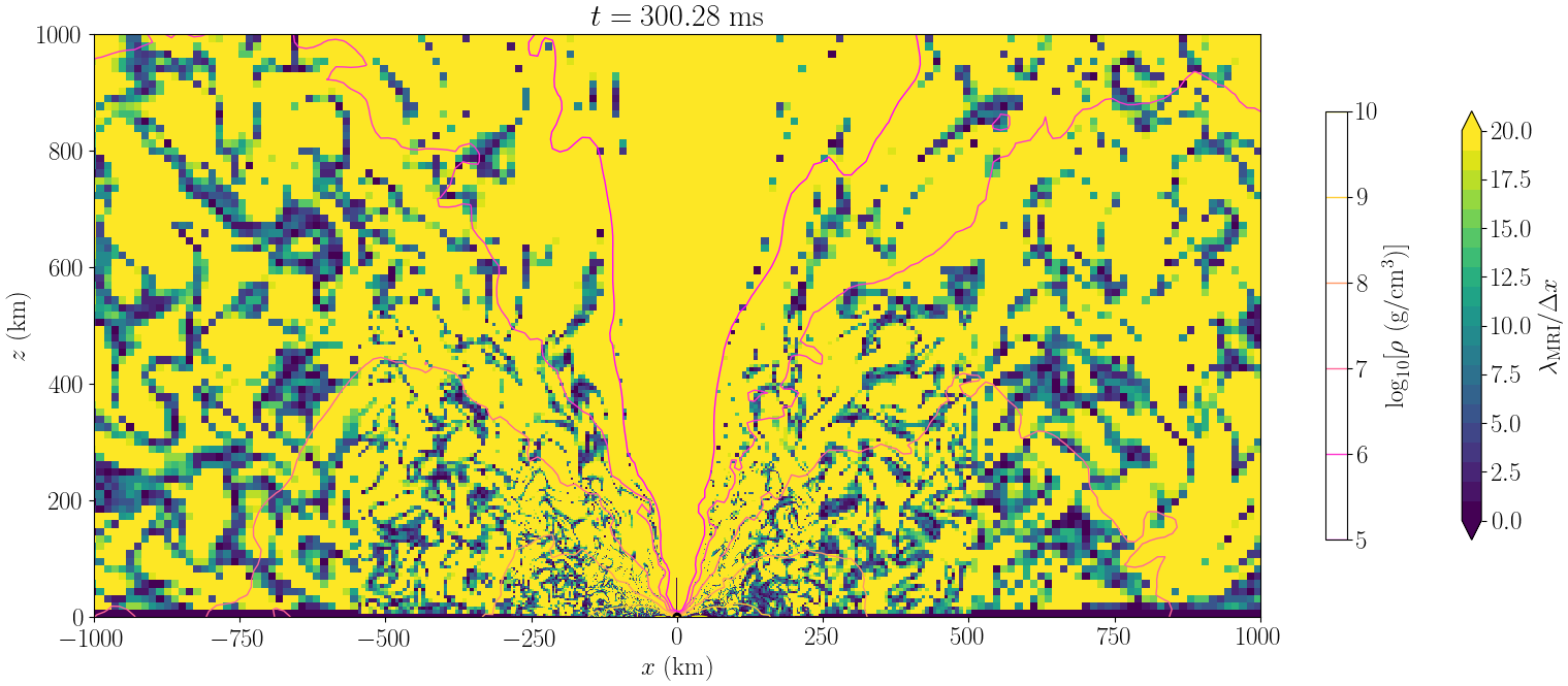
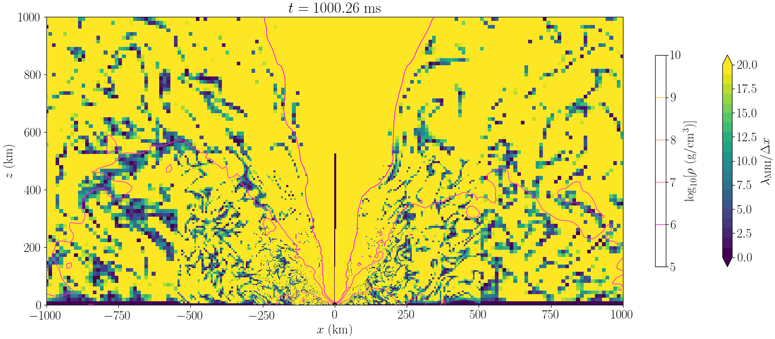
Figure 16: The snapshots of the MRI quality factor (color profile) together with the rest-mass density (contour) on the $x$-$z$ plane at $t\approx 300$ and 1000 ms for model Q4B5L.

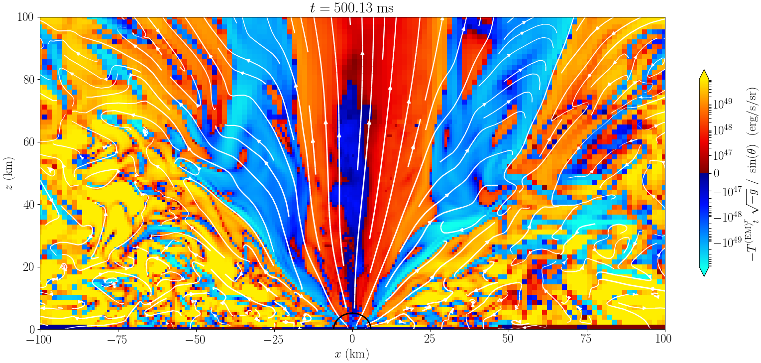
Figure 17: The snapshots of the outgoing Poynting flux per steradian (color profile) together with poloidal magnetic-field lines (white curves) near the apparent horizon on the $x$–$z$ plane at $t\approx 500$ and 1000 ms for model Q4B5L. The apparent horizon is shown with the black circle.

Figure 16 shows the snapshots of the MRI quality factor defined by ${\lambda_{z}}_{\rm MRI}/{\Delta}x$ on the $x$-$z$ plane for model Q4B5L. Here, ${\lambda_{z}}_{\rm MRI}$ is the wavelength of the fastest growing mode of the axisymmetric MRI, which is defined by

$${\lambda_{z}}_{\rm MRI} = \frac{b_{z}}{\sqrt{4{\pi}{\rho}h+b^{\mu}b_{\mu}}}\frac{2{\pi}}{\Omega},$$ (33)

where $\Omega$ denotes the local angular velocity and $z$-direction is the direction of the rotation axis. We note that for other time slices, the similar feature is also found. Figure 16 shows that the fastest growing mode is covered by more than 20 grid points in the large portion of the disk even for the low-resolution run (${\lambda_{z}}_{\rm MRI}\sim 10\,{\rm km}$ in the inner region of the disk), and thus, we consider that the fastest growing mode of the MRI is resolved with a reasonable accuracy in the present work.

Appendix D Evidence for the Blandford-Znajek mechanism

Figure 17 shows the snapshots for an outgoing Poynting flux per steradian near the apparent horizon defined by $-{T^{\mathrm{(EM)}}}^{~{}r}_{t}\sqrt{-g}/\sin{\theta}$. Along the poloidal magnetic-field line, the outgoing Poynting flux is distributed from the apparent horizon to the mangnetosphere around the rotational axis of the black hole. This indicates that energy is extracted from the black hole through the magnetic field, and thus, we can interpret that the Blandford-Znajek mechanism is in operation. In addition, we find that the total Poynting luminosity on the apparent horizon is $\sim 10^{49}\,{\rm erg/s}$. This value is consistent with the luminosity expected from the formula for the Blandford-Znajek mechanism Blandford and Znajek (1977) for the resultant values of the magnetic-field strength, black-hole mass, and spin.

References

- Abbott et al. (2016) B. P. Abbott et al. (LIGO Scientific Collaboration and Virgo Collaboration), Phys. Rev. Lett. 116, 061102 (2016).
- Abbott et al. (2021a) R. Abbott et al. (LIGO Scientific Collaboration and Virgo Collaboration), Phys. Rev. X 11, 021053 (2021a).
- Abbott et al. (2021b) R. Abbott et al., (2021b), arXiv:2111.03606 [gr-qc] .
- Abbott et al. (2017a) B. P. Abbott et al. (LIGO Scientific Collaboration and Virgo Collaboration), Phys. Rev. Lett. 119, 161101 (2017a).
- Abbott et al. (2017b) B. P. Abbott et al., Astrophys. J. 848, L12 (2017b).
- Abbott et al. (2017c) B. P. Abbott et al., Astrophys. J. 848, L13 (2017c).
- Abbott et al. (2021c) R. Abbott et al., Astrophys. J. 915, L5 (2021c).
- Shibata and Taniguchi (2011) M. Shibata and K. Taniguchi, Living Rev. Relativity 14, 6 (2011).
- Kyutoku et al. (2021) K. Kyutoku, M. Shibata, and K. Taniguchi, Living Rev. Relativity 24, 5 (2021).
- Eichler et al. (1989) D. Eichler, M. Livio, T. Piran, and D. N. Schramm, Nature (London) 340, 126 (1989).
- Nakar (2007) E. Nakar, Phys. Rep. 442, 166 (2007), the Hans Bethe Centennial Volume 1906-2006.
- Berger (2014) E. Berger, Annu. Rev. Astron. Astrophys. 52, 43 (2014).
- Lattimer and Schramm (1974) J. M. Lattimer and D. N. Schramm, Astrophys. J. Lett. 192, L145 (1974).
- Li and Paczyński (1998) L.-X. Li and B. Paczyński, Astrophys. J. 507, L59 (1998).
- Metzger et al. (2010) B. D. Metzger, G. Martínez-Pinedo, S. Darbha, E. Quataert, A. Arcones, D. Kasen, R. Thomas, P. Nugent, I. V. Panov, and N. T. Zinner, Mon. Not. R. Astron. Soc. 406, 2650 (2010).
- Shibata and Uryū (2006) M. Shibata and K. Uryū, Phys. Rev. D 74, 121503 (2006).
- Shibata and Uryū (2007) M. Shibata and K. Uryū, Classical Quantum Gravity 24, S125 (2007).
- Shibata and Taniguchi (2008) M. Shibata and K. Taniguchi, Phys. Rev. D 77, 084015 (2008).
- Etienne et al. (2008) Z. B. Etienne, J. A. Faber, Y. T. Liu, S. L. Shapiro, K. Taniguchi, and T. W. Baumgarte, Phys. Rev. D 77, 084002 (2008).
- Duez et al. (2008) M. D. Duez, F. Foucart, L. E. Kidder, H. P. Pfeiffer, M. A. Scheel, and S. A. Teukolsky, Phys. Rev. D 78, 104015 (2008).
- Shibata et al. (2009) M. Shibata, K. Kyutoku, T. Yamamoto, and K. Taniguchi, Phys. Rev. D 79, 044030 (2009).
- Etienne et al. (2009) Z. B. Etienne, Y. T. Liu, S. L. Shapiro, and T. W. Baumgarte, Phys. Rev. D 79, 044024 (2009).
- Chawla et al. (2010) S. Chawla, M. Anderson, M. Besselman, L. Lehner, S. L. Liebling, P. M. Motl, and D. Neilsen, Phys. Rev. Lett. 105, 111101 (2010).
- Duez et al. (2010) M. D. Duez, F. Foucart, L. E. Kidder, C. D. Ott, and S. A. Teukolsky, Classical Quantum Gravity 27, 114106 (2010).
- Kyutoku et al. (2010) K. Kyutoku, M. Shibata, and K. Taniguchi, Phys. Rev. D 82, 044049 (2010).
- Kyutoku et al. (2011) K. Kyutoku, H. Okawa, M. Shibata, and K. Taniguchi, Phys. Rev. D 84, 064018 (2011).
- Foucart et al. (2011) F. Foucart, M. D. Duez, L. E. Kidder, and S. A. Teukolsky, Phys. Rev. D 83, 024005 (2011).
- Foucart et al. (2012) F. Foucart, M. D. Duez, L. E. Kidder, M. A. Scheel, B. Szilagyi, and S. A. Teukolsky, Phys. Rev. D 85, 044015 (2012).
- Etienne et al. (2012a) Z. B. Etienne, Y. T. Liu, V. Paschalidis, and S. L. Shapiro, Phys. Rev. D 85, 064029 (2012a).
- Etienne et al. (2012b) Z. B. Etienne, V. Paschalidis, and S. L. Shapiro, Phys. Rev. D 86, 084026 (2012b).
- Kyutoku et al. (2013) K. Kyutoku, K. Ioka, and M. Shibata, Phys. Rev. D 88, 041503 (2013).
- Kyutoku et al. (2015) K. Kyutoku, K. Ioka, H. Okawa, M. Shibata, and K. Taniguchi, Phys. Rev. D 92, 044028 (2015).
- Foucart et al. (2013) F. Foucart, M. B. Deaton, M. D. Duez, L. E. Kidder, I. MacDonald, C. D. Ott, H. P. Pfeiffer, M. A. Scheel, B. Szilagyi, and S. A. Teukolsky, Phys. Rev. D 87, 084006 (2013).
- Lovelace et al. (2013) G. Lovelace, M. D. Duez, F. Foucart, L. E. Kidder, H. P. Pfeiffer, M. A. Scheel, and B. Szilágyi, Classical Quantum Gravity 30, 135004 (2013).
- Deaton et al. (2013) M. B. Deaton, M. D. Duez, F. Foucart, E. O’Connor, C. D. Ott, L. E. Kidder, C. D. Muhlberger, M. A. Scheel, and B. Szilagyi, Astrophys. J. 776, 47 (2013).
- Foucart et al. (2014) F. Foucart, M. B. Deaton, M. D. Duez, E. O’Connor, C. D. Ott, R. Haas, L. E. Kidder, H. P. Pfeiffer, M. A. Scheel, and B. Szilagyi, Phys. Rev. D 90, 024026 (2014).
- Paschalidis et al. (2015) V. Paschalidis, M. Ruiz, and S. L. Shapiro, Astrophys. J. 806, L14 (2015).
- Kawaguchi et al. (2015) K. Kawaguchi, K. Kyutoku, H. Nakano, H. Okawa, M. Shibata, and K. Taniguchi, Phys. Rev. D 92, 024014 (2015).
- Kiuchi et al. (2015) K. Kiuchi, Y. Sekiguchi, K. Kyutoku, M. Shibata, K. Taniguchi, and T. Wada, Phys. Rev. D 92, 064034 (2015).
- Foucart et al. (2017) F. Foucart, D. Desai, W. Brege, M. D. Duez, D. Kasen, D. A. Hemberger, L. E. Kidder, H. P. Pfeiffer, and M. A. Scheel, Classical Quantum Gravity 34, 044002 (2017).
- Kyutoku et al. (2018) K. Kyutoku, K. Kiuchi, Y. Sekiguchi, M. Shibata, and K. Taniguchi, Phys. Rev. D 97, 023009 (2018).
- Brege et al. (2018) W. Brege, M. D. Duez, F. Foucart, M. B. Deaton, J. Caro, D. A. Hemberger, L. E. Kidder, E. O’Connor, H. P. Pfeiffer, and M. A. Scheel, Phys. Rev. D 98, 063009 (2018).
- Ruiz et al. (2018) M. Ruiz, S. L. Shapiro, and A. Tsokaros, Phys. Rev. D 98, 123017 (2018).
- Foucart et al. (2019a) F. Foucart, M. D. Duez, T. Hinderer, J. Caro, A. R. Williamson, M. Boyle, A. Buonanno, R. Haas, D. A. Hemberger, L. E. Kidder, H. P. Pfeiffer, and M. A. Scheel, Phys. Rev. D 99, 044008 (2019a).
- Foucart et al. (2019b) F. Foucart, M. D. Duez, L. E. Kidder, S. M. Nissanke, H. P. Pfeiffer, and M. A. Scheel, Phys. Rev. D 99, 103025 (2019b).
- Hinderer et al. (2019) T. Hinderer, S. Nissanke, F. Foucart, K. Hotokezaka, T. Vincent, M. Kasliwal, P. Schmidt, A. R. Williamson, D. A. Nichols, M. D. Duez, L. E. Kidder, H. P. Pfeiffer, and M. A. Scheel, Phys. Rev. D 100, 063021 (2019).
- Hayashi et al. (2021) K. Hayashi, K. Kawaguchi, K. Kiuchi, K. Kyutoku, and M. Shibata, Phys. Rev. D 103, 043007 (2021).
- Foucart et al. (2021) F. Foucart, A. Chernoglazov, M. Boyle, T. Hinderer, M. Miller, J. Moxon, M. A. Scheel, N. Deppe, M. D. Duez, F. Hébert, L. E. Kidder, W. Throwe, and H. P. Pfeiffer, Phys. Rev. D 103, 064007 (2021).
- Chaurasia et al. (2021) S. V. Chaurasia, T. Dietrich, and S. Rosswog, Phys. Rev. D 104, 084010 (2021).
- Most et al. (2021) E. R. Most, L. J. Papenfort, S. D. Tootle, and L. Rezzolla, Mon. Not. R. Astron. Soc. 506, 3511 (2021).
- Fernández and Metzger (2013) R. Fernández and B. D. Metzger, Mon. Not. R. Astron. Soc. 435, 502 (2013).
- Metzger and Fernández (2014) B. D. Metzger and R. Fernández, Mon. Not. R. Astron. Soc. 441, 3444 (2014).
- Just et al. (2015) O. Just, A. Bauswein, R. A. Pulpillo, S. Goriely, and H.-T. Janka, Mon. Not. R. Astron. Soc. 448, 541 (2015).
- Fernández et al. (2015) R. Fernández, E. Quataert, J. Schwab, D. Kasen, and S. Rosswog, Mon. Not. R. Astron. Soc. 449, 390 (2015).
- Fernández et al. (2017) R. Fernández, F. Foucart, D. Kasen, J. Lippuner, D. Desai, and L. F. Roberts, Classical Quantum Gravity 34, 154001 (2017).
- Siegel and Metzger (2018) D. M. Siegel and B. D. Metzger, Astrophys. J. 858, 52 (2018).
- Fernández et al. (2019) R. Fernández, A. Tchekhovskoy, E. Quataert, F. Foucart, and D. Kasen, Mon. Not. R. Astron. Soc. 482, 3373 (2019).
- Janiuk (2019) A. Janiuk, Astrophys. J. 882, 163 (2019).
- Christie et al. (2019) I. M. Christie, A. Lalakos, A. Tchekhovskoy, R. Fernández, F. Foucart, E. Quataert, and D. Kasen, Mon. Not. R. Astron. Soc. 490, 4811 (2019).
- Miller et al. (2019) J. M. Miller, B. R. Ryan, J. C. Dolence, A. Burrows, C. J. Fontes, C. L. Fryer, O. Korobkin, J. Lippuner, M. R. Mumpower, and R. T. Wollaeger, Phys. Rev. D 100, 023008 (2019).
- Fujibayashi et al. (2020a) S. Fujibayashi, M. Shibata, S. Wanajo, K. Kiuchi, K. Kyutoku, and Y. Sekiguchi, Phys. Rev. D 101, 083029 (2020a).
- Fujibayashi et al. (2020b) S. Fujibayashi, M. Shibata, S. Wanajo, K. Kiuchi, K. Kyutoku, and Y. Sekiguchi, Phys. Rev. D 102, 123014 (2020b).
- Li and Siegel (2021) X. Li and D. M. Siegel, Phys. Rev. Lett. 126, 251101 (2021).
- Fernández et al. (2020) R. Fernández, F. Foucart, and J. Lippuner, Mon. Not. R. Astron. Soc. 497, 3221 (2020).
- Just et al. (2022) O. Just, S. Goriely, H. T. Janka, S. Nagataki, and A. Bauswein, Mon. Not. R. Astron. Soc. 509, 1377 (2022).
- Shibata et al. (2021) M. Shibata, S. Fujibayashi, and Y. Sekiguchi, Phys. Rev. D 104, 063026 (2021).
- Shibata and Nakamura (1995) M. Shibata and T. Nakamura, Phys. Rev. D 52, 5428 (1995).
- Baumgarte and Shapiro (1998) T. W. Baumgarte and S. L. Shapiro, Phys. Rev. D 59, 024007 (1998).
- Campanelli et al. (2006) M. Campanelli, C. O. Lousto, P. Marronetti, and Y. Zlochower, Phys. Rev. Lett. 96, 111101 (2006).
- Baker et al. (2006) J. G. Baker, J. Centrella, D.-I. Choi, M. Koppitz, and J. van Meter, Phys. Rev. Lett. 96, 111102 (2006).
- Marronetti et al. (2008) P. Marronetti, W. Tichy, B. Brügmann, J. González, and U. Sperhake, Phys. Rev. D 77, 064010 (2008).
- Hilditch et al. (2013) D. Hilditch, S. Bernuzzi, M. Thierfelder, Z. Cao, W. Tichy, and B. Brügmann, Phys. Rev. D 88, 084057 (2013).
- Shibata and Sekiguchi (2005) M. Shibata and Y. Sekiguchi, Phys. Rev. D 72, 044014 (2005).
- Shibata et al. (2007) M. Shibata, Y. Sekiguchi, and R. Takahashi, Prog. Theor. Phys. 118, 257 (2007).
- Kiuchi et al. (2012) K. Kiuchi, K. Kyutoku, and M. Shibata, Phys. Rev. D 86, 064008 (2012).
- Evans and Hawley (1988) C. R. Evans and J. F. Hawley, Astrophys. J. 332, 659 (1988).
- Balsara (2009) D. S. Balsara, J. Comput. Phys. 228, 5040 (2009).
- Sekiguchi et al. (2012) Y. Sekiguchi, K. Kiuchi, K. Kyutoku, and M. Shibata, Prog. Theor. Exp. Phys. 2012, 01A304 (2012).
- Thorne (1981) K. S. Thorne, Mon. Not. R. Astron. Soc. 194, 439 (1981).
- Shibata et al. (2011) M. Shibata, K. Kiuchi, Y. Sekiguchi, and Y. Suwa, Prog. Theor. Phys. 125, 1255 (2011).
- Fujibayashi et al. (2020c) S. Fujibayashi, S. Wanajo, K. Kiuchi, K. Kyutoku, Y. Sekiguchi, and M. Shibata, Astrophys. J. 901, 122 (2020c).
- Banik et al. (2014) S. Banik, M. Hempel, and D. Bandyopadhyay, Astrophys. J. 214, 22 (2014).
- Timmes and Swesty (2000) F. X. Timmes and F. D. Swesty, Astrophys. J. 126, 501 (2000).
- Miller et al. (2019) M. C. Miller, F. K. Lamb, A. J. Dittmann, S. Bogdanov, Z. Arzoumanian, K. C. Gendreau, S. Guillot, A. K. Harding, W. C. G. Ho, J. M. Lattimer, R. M. Ludlam, S. Mahmoodifar, S. M. Morsink, P. S. Ray, T. E. Strohmayer, K. S. Wood, T. Enoto, R. Foster, T. Okajima, G. Prigozhin, and Y. Soong, Astrophys. J. Lett. 887, L24 (2019).
- Balbus and Hawley (1991) S. A. Balbus and J. F. Hawley, Astrophys. J. 376, 214 (1991).
- Balbus and Hawley (1998) S. A. Balbus and J. F. Hawley, Rev. Mod. Phys. 70, 1 (1998).
- Masada and Sano (2008) Y. Masada and T. Sano, Astrophys. J. 689, 1234 (2008).
- Guilet et al. (2017) J. Guilet, A. Bauswein, O. Just, and H.-T. Janka, Mon. Not. R. Astron. Soc. 471, 1879 (2017).
- Brandenburg and Subramanian (2005) A. Brandenburg and K. Subramanian, Phys. Rep. 417, 1 (2005).
- Blandford and Payne (1982) R. D. Blandford and D. G. Payne, Mon. Not. R. Astron. Soc. 199, 883 (1982).
- Fuller et al. (1985) G. M. Fuller, W. A. Fowler, and M. J. Newman, Astrophys. J. 293, 1 (1985).
- Metzger et al. (2008) B. D. Metzger, A. L. Piro, and E. Quataert, Mon. Not. R. Astron. Soc. 390, 781 (2008).
- Liska et al. (2020) M. Liska, A. Tchekhovskoy, and E. Quataert, Mon. Not. R. Astron. Soc. 494, 3656 (2020).
- Blandford and Znajek (1977) R. D. Blandford and R. L. Znajek, Mon. Not. R. Astron. Soc. 179, 433 (1977).
- Shibata et al. (2006) M. Shibata, Y. T. Liu, S. L. Shapiro, and B. C. Stephens, Phys. Rev. D 74, 104026 (2006).
- Bardeen et al. (1972) J. M. Bardeen, W. H. Press, and S. A. Teukolsky, Astrophys. J. 178, 347 (1972).
- De and Siegel (2021) S. De and D. M. Siegel, Astrophys. J. 921, 94 (2021).
- Beloborodov (2003) A. M. Beloborodov, Astrophys. J. 588, 931 (2003).
- Hotokezaka et al. (2013) K. Hotokezaka, K. Kiuchi, K. Kyutoku, H. Okawa, Y. Sekiguchi, M. Shibata, and K. Taniguchi, Phys. Rev. D 87, 024001 (2013).
- Wanajo et al. (2014) S. Wanajo, Y. Sekiguchi, N. Nishimura, K. Kiuchi, K. Kyutoku, and M. Shibata, Astrophys. J. 789, L39 (2014).
- Kawaguchi et al. (2020) K. Kawaguchi, M. Shibata, and M. Tanaka, Astrophys. J. 889, 171 (2020).
- Tchekhovskoy et al. (2011) A. Tchekhovskoy, R. Narayan, and J. C. McKinney, Mon. Not. R. Astron. Soc. 418, L79 (2011).
- Uchida et al. (2017) H. Uchida, M. Shibata, T. Yoshida, Y. Sekiguchi, and H. Umeda, Phys. Rev. D 96, 083016 (2017).