Can we decipher the composition of the core of a neutron star?

Abstract

General relativity guarantees a unique one-to-one correspondence between static observables of neutron stars (NSs) accessible by multi-messenger astronomy, such as mass-radius or tidal deformability, and the equation of state (EoS) of beta equilibrated matter. It is well known that these static properties are not enough to discern conventional NSs from hybrid stars. However, if one assumes that hadrons present in the neutron star core are only neutrons and protons, the lepton fraction is in principle determined unequivocally by the condition of chemical equilibrium. Using a simple analytical method based on a polynomial expansion of the EoS, we show that multiple solutions are possible to the beta-equilibrium equation, leading to a characteristic indetermination on the composition of the interiors of NSs, even in the purely nucleonic hypothesis. We further show that additional empirical information on symmetric matter at high densities are not very efficient to pin down the composition, if uncertainties on measurements are accounted for. We conclude that constraints on the symmetry energy at high densities only, can make meaningful impact to decipher the composition of neutron star core. Our results give a lower limit to the uncertainty on the NS core composition that can be obtained with astrophysical and terrestrial experiments.

I Introduction

Neutron stars are among the most dense systems existing in the universe. Understanding the composition of their core will help us to peek at the behavior of matter at extreme density conditions. Unprecedented progress was achieved in multi-messenger astronomy in the last decade through quantitative measurements of neutron stars (NS) properties, such as mass measurements by radio astronomy through Shapiro delay Demorest et al. (2010); Antoniadis and et. al (2013), joint mass-radius determination by NICER using X-ray timing data Riley and et. al (2019); Miller and et. al. (2019); Riley and et. al. (2021); Miller and et. al (2021) or the tidal polarizability extracted from the gravitational wave signal by LIGO-Virgo collaboration Abbott and et. al. (2017, 2018, 2019); Aasi and et. al. (2015); Acernese and et. al. (2014).

A straightforward link between the observations and the underlying microphysics can be established due to a one-to-one correspondence between the static properties of NS and the EoS of matter under the realm of general relativity Hartle (1967). The behavior of the dense matter EoS can therefore be extracted with controlled uncertainty from the astrophysical observations within minimal assumptions using Bayesian techniques Steiner et al. (2013); Margueron et al. (2018a, b); Zhang et al. (2018); Lim and Holt (2019); Tsang et al. (2020); Traversi et al. (2020); Biswas et al. (2021); Essick et al. (2021). However, a major persisting challenge consists in connecting this empirically determined EoS with the internal properties of dense matter, notably to bring to light the existence (or absence) of hyperonic degrees of freedom and the deconfined quark matter in the core of neutron stars Burgio et al. (2021). Because of the well known “masquerade” phenomenon Alford et al. (2005), hybrid stars including a quark core can exhibit a mass-radius [$M$-$R$] relationship very similar to the one obtained for a star made of purely nucleonic matter, see Baym et al. (2018) for a recent review.

The discrimination between confined and deconfined matter in the NS core is clearly of foremost importance for our understanding of the QCD phase diagram. However, even in the simplified assumption of a purely nucleonic composition, a quantitative knowledge on the composition is of utmost importance. Indeed, the electron fraction in the star core is a crucial input both for differentiating the different nuclear theories, and to correctly model dynamical processes such as pulsar glitches, cooling and mergers Oertel et al. (2017); Potekhin and Chabrier (2018); Montoli, A. et al. (2020). Extraction of information on the composition from these dynamical processes is in principle possible, but it is clearly limited by the many microscopic and macroscopic unknowns in the complex theoretical modelling.

In the conventional density functional approaches, the energy functional fixes the composition a priori, when one solves the $\beta$-equilibrium condition equation to obtain the EoS of NS matter. Since the latter has a one-to-one connection to the NS $M$-$R$ relation, it is systematically assumed that, in the absence of exotic degrees of freedom, the uncertainty in the composition only arises from the error bar on the $M$-$R$ relation. However, we will demonstrate in this paper that the correspondence between the NS composition and the EoS, as it can be accessed through astrophysical observations, is not unique, even in the purely nucleonic hypothesis. This surprising result is due to the existence of multiple solutions to the $\beta$-equilibrium equation, which is analytically proved using two different realizations of the same EoS. The result is reinforced by a Bayesian analysis hypothesizing controlled uncertainties on the pressure of $\beta$-equilibrated matter at distinct number densities. Further, we made the analysis more realistic by extracting the EoS from an astrophysical measurement through the inversion of the Tolman-Oppenheimer-Volkoff (TOV) equation of hydrostatic equilibrium. We show that the propagation of uncertainties is such that the composition above twice the saturation density to be fully unconstrained, even if the EoS was pinned down very precisely. We tested independent complementary information from laboratory experiments at suprasaturation densities to extract meaningfully the proton fraction (or equivalently electron fraction) in the NS core and, consequently, the nuclear matter energy functional.

The plan of the paper is as follows. In Section II, we give the theoretical formalism based on the inversion of the $\beta$-equilibrium equation through an analytical polynomial expansion of the EoS in Section II.1, and different Bayesian schemes in Section II.2. Section III comprises the results from two approaches, first on the inversion of the baryonic EoS in Section III.1, and on a more realistic case of the $M$-$R$ relation in Section III.2. We explore the potential impact of laboratory constraints of the high density regime at fixed proton fraction, on the $\beta$-equilibrium composition in Section III.3. A brief summary and conclusions are drawn in Section IV.

II Inverting the $\beta$-equilibrium equation

II.1 Analytical approach

We consider purely nucleonic matter, characterized by its baryonic density $n$ and asymmetry $\delta=(n_{n}-n_{p})/n$, where $n_{n(p)}$ is the neutron (proton) density. In order to study the possibility of extracting the composition from the knowledge on the EoS, we take the beta-equilibrium energy functional from an arbitrary reference nuclear model $e_{th,\beta}(n)$, and solve the equilibrium equation for the composition $\delta_{\beta}(n)$:

$$\mu_{n}(n,\delta_{\beta})-\mu_{p}(n,\delta_{\beta})=\mu_{e}(n,\delta_{\beta}).$$ (1)

Here, the electron chemical potential is simply given by the Fermi energy: $\mu_{e}=\sqrt{(3\pi^{2}n_{e})^{2/3}+m_{e}^{2}}$ with $n_{e}=(n_{p}-n_{\mu})$ and $n_{\mu}$ the net muon density in the global equilibrium ($\mu_{\mu}=\mu_{e}$). The neutron and proton chemical potentials are given by:

$$\mu_{n,p}=\frac{\partial(ne_{th})}{\partial n_{n,p}}=e_{th}+m_{n,p}+n\left.\frac{\partial e_{th}}{\partial n}\right|_{\delta}\pm\left.\frac{\partial e_{th}}{\partial\delta}\right|_{n},$$ (2)

where $m_{n,p}$’s are the free nucleon masses. The quantity $e_{th}(n,\delta)$ is the energy per baryon that we want to reconstruct from the knowledge on $e_{th,\beta}(n)$ in a finite number of density points $n_{i},i=1,\dots,N$. Replacing Eq. (2) in Eq. (1) we immediately get:

$$2\left.\frac{\partial e_{th}(n,\delta_{\beta})}{\partial\delta}\right|_{n}=\mu_{e}(n,\delta_{\beta})-\Delta m_{np},$$ (3)

with $\Delta m_{np}=m_{n}-m_{p}$. To evaluate the l.h.s. of Eq. (3) in order to extract $\delta_{\beta}(n)$, we need to parametrize the functional out of the $\beta$-equilibrium trajectory. A convenient representation that can precisely reproduce any generic realistic nucleonic functional Margueron et al. (2018a), is given by the so called meta-model approach as,

$$e_{meta}(n,\delta)=t_{FG}^{*}(n,\delta)+U_{0}(n)+U_{sym}(n)\delta^{2}.$$ (4)

Here, $t_{FG}^{*}$ is a Fermi-gas type kinetic energy term which also takes into account the density dependence of the effective nucleon masses, and the deviation of the parabolic approximation of the symmetry energy Margueron et al. (2018a); $U_{0}(n)$ and $U_{sym}(n)$ can be attributed to the symmetric and asymmetric parts of the nuclear potential written as a Taylor’s expansion in density that, keeping up to 4th order, can be written as,

$$U_{0,sym}(n)=\sum_{k=0}^{4}\frac{(v_{k})_{0,sym}}{k!}x^{k},\ {with,}\ x=\frac{n-n_{sat}}{3n_{sat}},$$ (5)

where $(v_{k})_{0,sym}$ are functions of nuclear matter properties (NMPs) at saturation density $n_{sat}$ Margueron et al. (2018a). The NMPs needed for the meta-functional in Eq. (4) are the energy per particle $E_{sat}$, incompressibility $K_{sat}$, skewness $Q_{sat}$ and stiffness $Z_{sat}$ of symmetric nuclear matter (SNM), $e_{0}(n)=e_{th}(n,\delta=0)$; and symmetry energy $E_{sym}$, symmetry slope $L_{sym}$, symmetry incompressibility $K_{sym}$, symmetry skewness $Q_{sym}$ and symmetry stiffness $Z_{sym}$ corresponding to the density dependent symmetry energy, $e_{sym}(n)=(1/2)\partial^{2}e_{th}/\partial\delta^{2}(n,\delta=0)$, all evaluated at the equilibrium density of nuclear matter $n_{sat}$. The NMPs are connected to the successive derivatives of the energy functional at saturation in the isoscalar (symmetric matter $e_{0}$) and isovector (symmetry energy $e_{sym}$) sector. For the exact definitions of $(v_{k})_{0,sym}$ c.f. Eq. (21-31) of Ref. Margueron et al. (2018a).

Over the last three or four decades an enormous amount of theoretical and experimental works have been devoted to obtain the different nuclear matter properties. For example, the binding energy data of nuclei very well constrain $E_{sat}$ and $E_{sym}$ Möller et al. (2012); Jiang et al. (2012), giant monopole resonance energies limit the value of $K_{sat}$ Khan et al. (2012); De et al. (2015) and with some reasonable ambiguities $L_{sym}$ and $K_{sym}$ can be constrained by many different approaches Centelles et al. (2009); Roca-Maza et al. (2011); Abrahamyan and et al. (2012); Mondal et al. (2015, 2016); Chen and Piekarewicz (2014, 2015); Mondal et al. (2017, 2018); Reed et al. (2021). Since the lower order NMPs are relatively well constrained, for this analytical exercise we consider that they are known exactly in Eq. (4), and take the corresponding values of the reference model which we are trying to reproduce. However, the rest of the parameters $Q_{sat,sym}$ and $Z_{sat,sym}$ are not experimentally accessible, and scattered over a huge range of values across many different nuclear models Dutra et al. (2012, 2014).

These higher order parameters can be determined by equating the input $e_{th,\beta}(n)$ to its meta-model representation $e_{meta}(n,\delta_{\beta})$, at the asymmetry $\delta_{\beta}(n)$ corresponding to the solution of Eq. (3). Using the ansatz of Eq. (4) we arrive at the equation,

$$\frac{1}{6}x^{3}Q_{sat}+\frac{1}{24}x^{4}Z_{sat}+\frac{1}{6}x^{3}\delta_{\beta}^{2}Q_{sym}+\frac{1}{24}x^{4}{\delta_{\beta}}^{2}Z_{sym}$$

$$=e_{th,\beta}(n)-e_{meta}^{0}(n,{\delta}_{\beta}),$$ (6)

where $e_{meta}^{0}$ is the functional $e_{meta}$ from Eq. (4) obtained by setting the lower order NMPs from the input functional, and $Q_{sat,sym}=Z_{sat,sym}=0$. The simultaneous solution of Eq. (6) and (3) can be obtained with a simple iterative matrix inversion by inputting the values of $e_{th,\beta}(n_{i})$ corresponding to four distinct density points $i=1,\dots,4$ as:

$$\left[\begin{array}[]{c}Q_{sat}\\ Z_{sat}\\ Q_{sym}\\ Z_{sym}\end{array}\right]=24\left[\begin{array}[]{cccc}4x_{1}^{3}&x_{1}^{4}&4x_{1}^{3}\delta_{1}^{2}&x_{1}^{4}\delta_{1}^{2}\\ 4x_{2}^{3}&x_{2}^{4}&4x_{2}^{3}\delta_{2}^{2}&x_{2}^{4}\delta_{2}^{2}\\ 4x_{3}^{3}&x_{3}^{4}&4x_{3}^{3}\delta_{3}^{2}&x_{3}^{4}\delta_{3}^{2}\\ 4x_{4}^{3}&x_{4}^{4}&4x_{4}^{3}\delta_{4}^{2}&x_{4}^{4}\delta_{4}^{2}\end{array}\right]^{-1}\left[\begin{array}[]{c}e_{1}\\ e_{2}\\ e_{3}\\ e_{4}\end{array}\right],$$ (7)

with $e_{i}=e_{th,\beta}(n_{i})-e_{meta}^{0}(n_{i},{\delta}_{i})$, and $\delta_{i}$ the solution of the meta-model equivalent of Eq.(3):

$$2\left.\frac{\partial e_{meta}(n_{i},\delta)}{\partial\delta}\right|_{n_{i}}=\mu_{e}(n_{i},\delta)-\Delta m_{np}.$$ (8)

The solution of the coupled equations (8), (4) and (7) fully determines the functional $e_{meta}$ that by construction coincides with the reference model in $\beta$-equilibrium, at the four chosen density points. Possible multiple solutions of the $\beta$-equilibrium equation can then be sought out, by slightly varying the chosen density points, or modifying the initialization of the iterative procedure, resulting in different $Q_{sat,sym}$ and $Z_{sat,sym}$. Such multiple solutions arise from the indetermination of the high order NMPs $Q_{sat,sym}$ and $Z_{sat,sym}$. If we consider that parameters such as $L_{sym}$ and $K_{sym}$ are not sufficiently pinned down as well, the procedure of Section II.1 could also be extended to a higher set of NMPs by increasing the number of density points in Eq.(7). For this reason, in the Bayesian approach presented in the next Section, we have also added the relatively poorly constrained $K_{sym}$ parameter to our prior. However, we have checked that adding an extra dimension to Eq.(7) including $K_{sym}$ does not change the results of Section III.

II.2 Bayesian approach

In the astrophysical context, the EoS of dense matter is not directly measured at different density points; they are rather inferred from the mass, tidal polarizability and radius through the structural equations of the star in general relativity, which imply an integration of the $\beta$-equilibrated EoS over the whole star density profile. Moreover, the observational quantities are known with finite precision, inducing an uncertainty that propagates to the EoS, and might blur the correlation between the EoS and the energy functional and composition as given by the matrix inversion in Eq. (7). To account for this limitation, we attempt a reconstruction of the reference model from the general meta-functional Eq. (4) through a Bayesian approach, where we sample the prior keeping fixed the lower order parameters (which are considered as “known” from independent measurements) $E_{sat},K_{sat},E_{sym}$ and $L_{sym}$ to the corresponding model values. The rest of the parameters $K_{sym}$, $Q_{sat,sym}$ and $Z_{sat,sym}$ are populated in a Monte-Carlo sampling with a flat distribution as $K_{sym}=[-400,200]$, $Q_{sat}=[-1000,1000]$, $Q_{sym}=[-2000,2000]$, $Z_{sat}=[-5000,5000]$, $Z_{sym}=[-5000,5000]$, all in units of MeV. These ranges are chosen such as to include a large number of popular relativistic as well as non-relativistic functionals Margueron et al. (2018a); Dinh Thi et al. (2021). We have checked that the arbitrary choice of the reference model does not play any significant role in the qualitative results presented in this paper.

The posterior distributions of the set ${\bf X}\equiv\{K_{sym},Q_{sat},Q_{sym},Z_{sat},Z_{sym}\}$ of EoS parameters are conditioned by likelihood models of the different observations and constraints $\mathbf{c}$ according to the standard definition:

$$P({\mathbf{X}}|{\mathbf{c}})=\mathcal{N}P({\mathbf{X}})\prod_{k}P(c_{k}|{\mathbf{X}}),$$ (9)

where $P({\mathbf{X}})$ is the prior, and $\mathcal{N}$ is a normalization factor. Posterior distributions of different observables $Y$ are calculated by marginalizing over the EoS parameters as:

$$P(Y|{\mathbf{c}})=\prod_{k=1}^{M}\int_{X_{k}^{min}}^{X_{k}^{max}}dX_{k}\,P({\mathbf{X}}|{\mathbf{c}})\delta\left(Y-Y({\mathbf{X}})\right),$$ (10)

where $M=5$ is the number of parameters in the meta-model which are varied. $Y({\mathbf{X}})$ is the value of any observable $Y$ obtained with the ${\mathbf{X}}$ parameter set along with the fixed lower order parameters, with $X_{k}^{\rm min(max)}$ being the minimum (maximum) value in the prior distribution taken for the analysis. The constraints $c_{k}$ are pseudo-observations from the reference model FSU2. We will successively consider different choices for the pseudo-observations, leading to four different posterior distributions:

• post-1 - The total equilibrium pressure $P_{th}$ of the reference model is imposed at four different density points, as in the analytical inversion presented in Section II.1. No uncertainty is considered on the baryonic density, and the likelihood model is a Gaussian distribution with $\sigma_{P}/P_{th}=0.1$ .

• post-2 - Three hypothetical radii measurements at fixed NS mass are imposed, where the 1-$\sigma$ uncertainty is arbitrarily fixed to 5% of the model values: $R_{1.4M_{\odot}}$, $R_{1.7M_{\odot}}$ and $R_{2.01M_{\odot}}$.

• post-3 - The pseudo-observations of radii of post-2 are complemented with a hypothetical SNM pressure observation at $4n_{sat}$ calculated from the reference model with 10% precision.

• post-4 - An extra constraint is further imposed on top of post-3 as the theoretical value of the symmetry energy at $4n_{sat}$, again with 10% precision.

III Results

The determination of the energy functional and matter composition from the inversion of the $\beta$ equilibrium information as explained in Section II is illustrated using the relativistic mean field (RMF) model FSU2 Chen and Piekarewicz (2014) as the reference model, including nucleons, electrons and muons. We have repeated all the calculations shown in this paper using the BSK24Goriely (2015), the Sly4Chabanat et al. (1998), and the SINPAMondal et al. (2016) models. Though the quantitative predictions are obviously different, all the qualitative results presented in the paper are independent of the choice of the reference model.

III.1 Constraining the pressure of $\beta$-equilibrated matter

To illustrate the existence of multiple solutions to the $\beta$ equilibrium equation, and validate the Bayesian approach, we first consider the academic situation of post-1, where the pseudo-observations are the values of the FSU2 equilibrium pressure at different density points, chosen to be similar $n_{i}$, $i=1,\dots,4$ used for the analytical inversion in Eq.(7), with an arbitrarily chosen 10% precision.

Figure 1: (Color online) Pressure (panel a) and electron fraction (panel b) for $\beta$-equilibrated matter as a function of density for FSU2 and its meta-model equivalents “$\beta$-eq.” and “$\beta$-eq.+lab” along with its prior and posterior distributions with different confidence intervals (CI) calculated from “post-1” (see text for details).

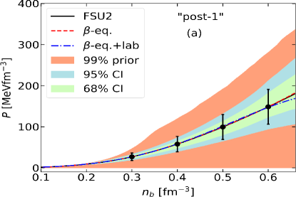
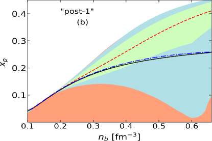
In Fig. 1 the NS EoS calculated from FSU2 is given by the black line. The corresponding red-dashed, and blue dashed-dotted lines give two different meta-model equivalents of FSU2 produced with Eq. (7). The red dashed lines (“$\beta$-eq.”) are obtained by considering initial guess values for the parameters $Q_{sat}=Z_{sat}=Q_{sym}=Z_{sym}=0$, while the functional described by the blue dashed-dotted line (“$\beta$-eq.+lab”) is obtained if $Q_{sat}$ and $Z_{sat}$ are initialized to the values that exactly reproduce the SNM energy and pressure of FSU2 at $n=4n_{sat}$ [see Section III.3 and Eq.(11)]. The two extremities of density points chosen to obtain the “$\beta$-eq.” and “$\beta$-eq.+lab” solutions are the central densities corresponding to NSs with mass $1.4M_{\odot}$ and $2.01M_{\odot}$ in FSU2, with two more equispaced points in between for the former i.e. “$\beta$-eq.”. The coherence between the three lines in the upper panel of Fig. 1 shows the absolute compatibility between FSU2 and its meta-model equivalents, as far as the $\beta$-equilibrium EoS is concerned. However, if we turn to the composition (Fig. 1(b)) , we observe a strong deviation between the model (black line) compared to the “$\beta$-eq.” solution (red dashed line), pointing towards multiple solutions of the $\beta$-equilibrium equation.

The corresponding Bayesian analysis “post-1” also supports this toy model calculation. In Figure 1, the 68% and 95% posteriors on the pressure and proton fraction, along with the 99% prior are plotted as green, blue and orange bands, respectively. We observe that the posterior for pressure is correctly centered on the reference model EoS, but the uncertainty in the composition covers the whole physical range of $x_{p}$, with the highest probability concentrated on the solution given by the functional solution that is not compatible with the reference FSU2 functional. The compatibility of the Bayesian analysis with the “$\beta$-eq.” solution is most likely due to the fact that we have arbitrarily centered around zero in the prior distribution of the unknown high order NMPs. However, a more educated guess is difficult to justify given the absence of direct constraints on those quantities.

III.2 Constraining the $M$-$R$ relation

As already discussed in Section II.2, realistic experimental constraints on the nuclear functional are given by the observation of integrated quantities such as the mass, the radius, or the tidal polarizability of NSs. We therefore turn to the post-2 protocol, where three hypothetical radii measurements at fixed NS masses are imposed, centered on the FSU2 theoretical value: $R_{1.4M_{\odot}}=14.18\pm 0.71$ km, $R_{1.7M_{\odot}}=13.79\pm 0.69$ km and $R_{2.01M_{\odot}}=12.93\pm 0.65$ km. In Fig. 2(a), these are denoted by the vertical black error bands on the FSU2 $M$-$R$ curve (black line). The corresponding 68% and 95% posteriors on the radii, accompanied by 99% prior are plotted as green, blue and orange bands, respectively. The accuracy on the posteriors obtained in the Bayesian analysis conditioned on $M$-$R$, is similar to the one obtained by directly imposing the EoS behavior as in post-1.

Figure 2: (Color online) Radius versus mass (panel a), Pressure (panel b) and proton fraction (panel c) versus density for FSU2 and its meta-model equivalents, along with its prior and posterior distributions with different confidence intervals (CI) calculated from “post-2” (see text for details).

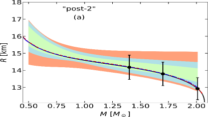
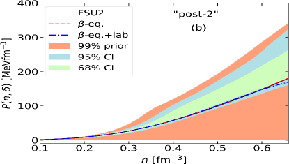
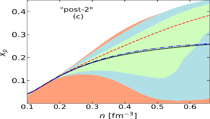
The 5% error bar on the pseudo-observations converts into $\approx 20$% uncertainty in the high density EoS, as displayed in Fig. 2(b). This is due to the well known non-linearity of the relation between $M$-$R$ and EoS, as given by the TOV equation. We can also observe a systematic shift compared to the “true” values towards higher pressure as the density increases, with a corresponding shift in the radius, increasing with increasing NS mass. This behavior is expected in any Bayesian analysis, if the prior is not centered on the true value. We can also see that the width of the posterior $M$-$R$ band is thinner than the hypothetical measurement. This can be appreciated from the fact that the separate radii measurements effectively constrain the same parameters, leading to a stronger constraint than any individual measurement. Moreover, the strong assumption of an exact knowledge of the low density physics encoded in the lower order parameters in Eq. (4) strongly constrains the EoS up to $\sim 2n_{sat}$, as seen in Fig. 1. The fact that only the higher order parameters are varied is not sufficient to eliminate the global bias observed, but it contributes to narrow the posterior prediction.

All in all, the true EoS is recovered at the 1-$\sigma$ level, which can be considered as a very satisfactory EoS determination. This is an illustration of the well know fact that a precise measurement of NS radii is an extremely powerful EoS estimator. However, the posterior distribution of the proton fraction is very similar to the one observed in Figure 1, and the uncertainty in the composition covers the whole physical range of $x_{p}$. This confirms the observations of Section III.1, namely the uncertainty in the composition appears not to be due to the imprecision in the knowledge of the EoS, but rather to the degeneracy between very different energy functionals that happen to lead to the same $\beta$-equilibrium trajectory due to cancellations between the symmetric matter $U_{0}$ and the symmetry $U_{sym}$ functionals (see Eq. (4)).

III.3 Constraining the SNM and symmetry energy

The results of Fig. 2 suggest that, to eliminate the degeneracy and pin down the behavior of the reference model, independent additional constraints are needed from either the symmetric or the asymmetric part of the functional to complement the astrophysical observations. This argument is confirmed by the fact that the analytical EoS inversion presented in Section II.1 systematically leads to the correct reproduction of the reference functional even in the composition, if the $\beta$-equilibrium information is only used to extract the NMPs associated to the symmetry energy. In particular, we consider a high density point that we fix for illustrative purposes at $n=4n_{sat}$, and impose the meta-functional in Eq. (4) to exactly reproduce the SNM energy and pressure of the reference model. This fixes the parameters $Q_{sat}$ and $Z_{sat}$ Margueron et al. (2018a). We then follow the same method of matrix inversion as in Eq.(7) to extract $Q_{sym}$ and $Z_{sym}$ as the following,

$$\frac{1}{6}x^{3}{\delta_{\beta}}^{2}Q_{sym}+\frac{1}{24}x^{4}{\delta_{\beta}}^{2}Z_{sym}=e_{th}(n,\delta_{\beta})-e_{meta}^{0,sat}(n,{\delta_{\beta}}),$$ (11)

where $e_{meta}^{0,sat}$ is the functional $e_{meta}$ from Eq. (4) obtained by using the lower order NMPs from the input functional, $Q_{sat}$ and $Z_{sat}$ from the method described above and $Q_{sym}=Z_{sym}=0$. Here, we need only two density points, which we have chosen as the central densities of FSU2 corresponding to NSs of masses 1.4$M_{\odot}$ and 2.01$M_{\odot}$. As expected, among the different possible solutions of the $\beta$-equilibrium equation, this strategy selects the meta-functional that correctly reproduces the reference model both in the isoscalar and in the isovector sector (“$\beta$-eq.+lab”), represented by dot-dashed blue lines in Figs.1-2.

Figure 3: (Color online) Energy for symmetric nuclear matter $e_{0}$ (panel a) and symmetry energy $e_{sym}$ (panel b) as a function of number density for FSU2 and its meta-model equivalents “$\beta$-eq.” and “$\beta$-eq.+lab” are displayed.

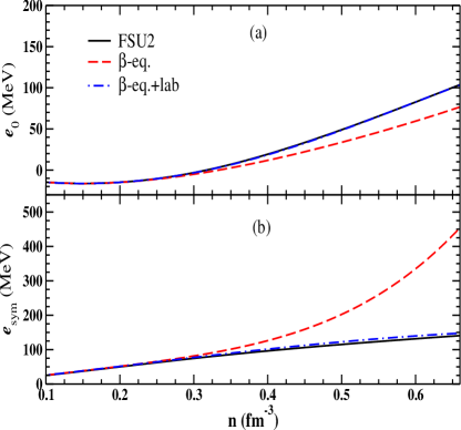
In Fig. 3, we display the behavior of SNM ($e_{0}$ in panel a) and symmetry energy ($e_{sym}$ in panel b) as a function of number density $n$ for the reference model FSU2 in conjunction with “$\beta$-eq.” and “$\beta$-eq.+lab” meta-model equivalents represented by black solid, red-dashed and blue dash-dotted lines, respectively. One can notice that even though “$\beta$-eq.” solution doesn’t match with $e_{0}$ and $e_{sym}$ of FSU2, it perfectly reproduces the $\beta$-equilibrium pressure (Fig. 1(a)). This explains the mismatch between the red-dashed and black solid lines in the composition (Fig. 1(b) and Fig. 2(c)). However, for obvious reasons “$\beta$-eq.+lab” solution agrees everywhere with FSU2 in Figs.1-2 as it correctly reproduces the SNM and symmetry energy behavior separately (see Fig. 3).

Information on the energy and pressure of symmetric matter at suprasaturation density is expected from upcoming measurements in relativistic heavy-ion collisions Adamczewski-Musch and et. al. (2020). However, we expect those constraints to be affected by considerable uncertainties like any other measurements. To understand their effect on the determination of the composition, we perform a similar Bayesian analysis as before (“post-3”), by complementing the pseudo-observations of radii introduced earlier, with a hypothetical SNM pressure observation at $4n_{sat}$ calculated from FSU2 with 10% precision i.e. $P_{SNM}(0.6{\rm\ fm}^{-3})=125.14\pm 12.51$ MeV.

Figure 4: (Color online) Proton fraction $x_{p}$ as a function of density to compare the distributions “post-3” (panel (a)) and “post-4” (panel (b)) (see text for details).

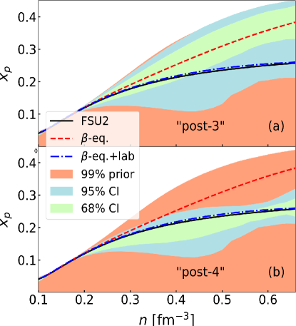
The resulting posterior proton fraction $x_{p}$ as a function of density $n$ is displayed in Fig. 4(a). One can notice that the distribution is less disperse, but it is still centered around the wrong composition described earlier (dashed red line). The mismatch can be understood as follows. The energy of the $\beta$-equilibrated matter in Eq. (3) is determined by an interplay between energy of SNM and symmetry energy. Those quantities are not independent, since the relative proportion of the two is imposed by the $\beta$-equilibrium equation, but the latter possesses multiple solutions. In the case of the blue dash-dotted lines in Fig. 4, the symmetric matter NMPs are fitted exactly to their true values, which forces the symmetry energy and $x_{p}$ to take their model values (see Fig. 3). But in “post-3”, the SNM is not fixed exactly, which leaves a leeway for errors to creep in and get transferred further to symmetry energy and $x_{p}$ because of the intrinsic degeneracy between the two parts of the functional. This interpretation is in agreement with previous studies Xie and Li (2019, 2020); Li et al. (2021). To better quantify the statement, we add another constraint on top of “post-3” by further imposing the symmetry energy of FSU2 at $4n_{sat}$ as: $e_{sym}(0.6{\rm\ fm}^{-3})=131.65\pm 13.{16}$ MeV, which is coined as “post-4”. We plot the proton fraction $x_{p}$ as a function of density for “post-4” in Fig. 4(b), and the 68% posterior of the Bayesian analysis gets aligned with the true composition, albeit with a non-negligible amount of uncertainty associated with it.

The different sensitivity of $x_{p}$ to $e_{\beta}$, $e_{0}$ and $e_{sym}$ can be qualitatively understood via analytical uncertainty propagation. If we employ a simple parabolic approximation for the symmetry energy $e_{\beta}\approx e_{0}+e_{sym}\delta_{\beta}^{2}$, Eq. (3) can be written in terms of the proton fraction as,

$$4(1-2x_{p})e_{sym}-\Delta m_{np}=\mu_{e}(x_{p}).$$ (12)

In the ultra-relativistic approximation for the electron gas, one can easily write the uncertainty in proton fraction $\Delta x_{p}$ in terms of uncertainties on $\beta$-equilibrium energy $\Delta e_{\beta}$ and SNM energy $\Delta e_{0}$, or on symmetry energy $\Delta e_{sym}$ as

$$\Delta x_{p}\approx\frac{12x_{p}(\Delta e_{\beta}+\Delta e_{0})}{\mu_{e}|1-8x_{p}|}\approx\frac{12(1-2x_{p})^{2}x_{p}\Delta e_{sym}}{\mu_{e}(4x_{p}+1)}.$$ (13)

Figure 5: (Color online) Uncertainty on the symmetry energy $\Delta e_{sym}$ as a function of density (panel (a)), its consequence on the uncertainties of proton fraction $\Delta x_{p}$ as a function of density (panel (c)) along with $\Delta x_{p}$ caused due to uncertainties in $\beta$-equilibrated energy $\Delta e_{\beta}$ and SNM energy $\Delta e_{0}$ (panel (b)), all obtained from Eq. (13) (see text for details).

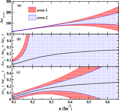
The first equality in Eq. (13) reflects the situation of “post-3” and the second one of “post-4”. As a qualitative estimate of the present uncertainty in the symmetry energy, we consider the uncertainties in the NMPs proposed in Table IX of Ref. Margueron et al. (2018a). In Fig. 5(a) we plot this (red band) as a function of density $n$. The thinner blue band is simply half of it. Concerning $\Delta e_{\beta}$ and $\Delta e_{0}$, we take the conservative choice $\Delta e_{\beta}+\Delta e_{0}=\Delta e_{sym}$, such as to concentrate on the different uncertainty propagation due to the form of the $\beta$-equilibrium equation, independent of the actual precision of the measurements. The results are shown in Fig. 5(b) and (c). One can see that the error band on $\Delta x_{p}$ spans the whole space in Fig. 5(b), at variance with Fig. 5(c). This can qualitatively explain the findings of our Bayesian analyses “post-3” and “post-4” of Fig. 4, pointing to the fact that the knowledge on symmetry energy at high density plays stronger role in determining the proton fraction inside the core of a NS, than an equivalent information on SNM. It is worthwhile to pose a caution on the information derived from Eq. 13. The apparent divergence in $\Delta x_{p}$ at $x_{p}=0.125$ is an artifact of the simplistic way to extract the error from the approximate $\beta$-equilibrium relation Eq.(12). However, a smooth removal of the divergence still engulfs the whole available space of proton fraction $x_{p}$ in Fig. 5(b).

IV Summary and Conclusions

In summary, we have analyzed the amount of empirical information which is needed to decipher the composition of the core of a catalyzed non-rotating neutron star within the nucleonic hypothesis. Using both a quasi-analytical inversion of the $\beta$-equilibrium equation, and a more quantitative Bayesian analysis, we have shown that one can land in a wrong conclusion on the composition relying only on astrophysical informations coming from static properties of neutron star.

In an ideal situation, where one knows all the NMPs up to second order exactly, the composition can be extracted by providing exact information on the energy per nucleon of SNM at a single high density point. However, if uncertainties are taken into account even moderately, the core proton fraction is fully unconstrained unless the astrophysical observations are complemented with accurate measurements on the symmetry energy at high density.

Finally, it is important to mention that this study gives only a lower limit on the accessible uncertainty to the composition of neutron star interior. Further uncertainties will arise from the possible incorporation of exotic degrees of freedom e.g. hyperons or the deconfined quark matter, which are kept out in the present study.

Acknowledgement- The authors acknowledge partial support from the IN2P3 Master Project “NewMAC”.

References

- Demorest et al. (2010) P. Demorest, T. Pennucci, S. Ransom, M. Roberts, and J. Hessels, Nature 467, 1081 (2010).
- Antoniadis and et. al (2013) J. Antoniadis and et. al, Science 340, 1233232 (2013).
- Riley and et. al (2019) T. E. Riley and et. al, Astrophys. J. 887, L21 (2019).
- Miller and et. al. (2019) M. C. Miller and et. al., Astrophys. J. 887, L24 (2019).
- Riley and et. al. (2021) T. E. Riley and et. al., Astrophys. J. 918, L27 (2021).
- Miller and et. al (2021) M. C. Miller and et. al, Astrophys. J. 918, L28 (2021).
- Abbott and et. al. (2017) B. P. Abbott and et. al. (LIGO Scientific Collaboration and Virgo Collaboration), Phys. Rev. Lett. 119, 161101 (2017).
- Abbott and et. al. (2018) B. P. Abbott and et. al. (The LIGO Scientific Collaboration and the Virgo Collaboration), Phys. Rev. Lett. 121, 161101 (2018).
- Abbott and et. al. (2019) B. P. Abbott and et. al. (LIGO Scientific Collaboration and Virgo Collaboration), Phys. Rev. X 9, 011001 (2019).
- Aasi and et. al. (2015) J. Aasi and et. al., Classical and Quantum Gravity 32, 074001 (2015).
- Acernese and et. al. (2014) F. Acernese and et. al., Classical and Quantum Gravity 32, 024001 (2014).
- Hartle (1967) J. B. Hartle, Astrophys. J. 150, 1005 (1967).
- Steiner et al. (2013) A. W. Steiner, J. M. Lattimer, and E. F. Brown, Astrophys. J. 765, L5 (2013).
- Margueron et al. (2018a) J. Margueron, R. Hoffmann Casali, and F. Gulminelli, Phys. Rev. C 97, 025805 (2018a).
- Margueron et al. (2018b) J. Margueron, R. Hoffmann Casali, and F. Gulminelli, Phys. Rev. C 97, 025806 (2018b).
- Zhang et al. (2018) N.-B. Zhang, B.-A. Li, and J. Xu, Astrophys. J. 859, 90 (2018).
- Lim and Holt (2019) Y. Lim and J. W. Holt, The European Physical Journal A 55, 11 (2019).
- Tsang et al. (2020) C. Y. Tsang, M. B. Tsang, P. Danielewicz, W. G. Lynch, and F. J. Fattoyev, Phys. Rev. C 102, 045808 (2020).
- Traversi et al. (2020) S. Traversi, P. Char, and G. Pagliara, Astrophys. J. 897, 165 (2020).
- Biswas et al. (2021) B. Biswas, P. Char, R. Nandi, and S. Bose, Phys. Rev. D 103, 103015 (2021).
- Essick et al. (2021) R. Essick, I. Tews, P. Landry, and A. Schwenk, Phys. Rev. Lett. 127, 192701 (2021).
- Burgio et al. (2021) G. F. Burgio, H.-J. Schulze, I. Vidaña, and J. B. Wei, Progress in Particle and Nuclear Physics 120, 103879 (2021).
- Alford et al. (2005) M. Alford, M. Braby, M. Paris, and S. Reddy, Astrophys. J. 629, 969 (2005).
- Baym et al. (2018) G. Baym, T. Hatsuda, T. Kojo, P. D. Powell, Y. Song, and T. Takatsuka, Reports on Progress in Physics 81, 056902 (2018).
- Oertel et al. (2017) M. Oertel, M. Hempel, T. Klähn, and S. Typel, Rev. Mod. Phys. 89, 015007 (2017).
- Potekhin and Chabrier (2018) A. Y. Potekhin and G. Chabrier, A&A 609, A74 (2018).
- Montoli, A. et al. (2020) Montoli, A., Antonelli, M., Magistrelli, F., and Pizzochero, P. M., A&A 642, A223 (2020).
- Möller et al. (2012) P. Möller, W. D. Myers, H. Sagawa, and S. Yoshida, Phys. Rev. Lett 108, 052501 (2012).
- Jiang et al. (2012) H. Jiang, G. J. Fu, Y. M. Zhao, and A. Arima, Phys. Rev. C 85, 024301 (2012).
- Khan et al. (2012) E. Khan, J. Margueron, and I. Vidaña, Phys. Rev. Lett. 109, 092501 (2012).
- De et al. (2015) J. N. De, S. K. Samaddar, and B. K. Agrawal, Phys. Rev. C 92, 014304 (2015).
- Centelles et al. (2009) M. Centelles, X. Roca-Maza, X. Viñas, and M. Warda, Phys. Rev. Lett. 102, 122502 (2009).
- Roca-Maza et al. (2011) X. Roca-Maza, M. Centelles, X. Viñas, and M. Warda, Phys. Rev. Lett. 106, 252501 (2011).
- Abrahamyan and et al. (2012) S. Abrahamyan and et al., Phys. Rev. Lett. 108, 112502 (2012).
- Mondal et al. (2015) C. Mondal, B. K. Agrawal, and J. N. De, Phys. Rev. C 92, 024302 (2015).
- Mondal et al. (2016) C. Mondal, B. K. Agrawal, J. N. De, and S. K. Samaddar, Phys. Rev. C 93, 044328 (2016).
- Chen and Piekarewicz (2014) W.-C. Chen and J. Piekarewicz, Phys. Rev. C 90, 044305 (2014).
- Chen and Piekarewicz (2015) W.-C. Chen and J. Piekarewicz, Phys. Lett. B 748, 284 (2015).
- Mondal et al. (2017) C. Mondal, B. K. Agrawal, J. N. De, S. K. Samaddar, M. Centelles, and X. Viñas, Phys. Rev. C 96, 021302(R) (2017).
- Mondal et al. (2018) C. Mondal, B. K. Agrawal, J. N. De, and S. K. Samaddar, International Journal of Modern Physics E 27, 1850078 (2018).
- Reed et al. (2021) B. T. Reed, F. J. Fattoyev, C. J. Horowitz, and J. Piekarewicz, Phys. Rev. Lett. 126, 172503 (2021).
- Dutra et al. (2012) M. Dutra, O. Lourenço, J. S. Sá Martins, A. Delfino, J. R. Stone, and P. D. Stevenson, Phys. Rev. C 85, 035201 (2012).
- Dutra et al. (2014) M. Dutra, O. Lourenço, S. S. Avancini, B. V. Carlson, A. Delfino, D. P. Menezes, C. Providência, S. Typel, and J. R. Stone, Phys. Rev. C 90, 055203 (2014).
- Dinh Thi et al. (2021) H. Dinh Thi, C. Mondal, and F. Gulminelli, Universe 7, 373 (2021).
- Goriely (2015) S. Goriely, Nuclear Physics A 933, 68 (2015).
- Chabanat et al. (1998) E. Chabanat, P. Bonche, P. Haensel, J. Meyer, and R. Schaeffer, Nucl. Phys. A635, 231 (1998).
- Adamczewski-Musch and et. al. (2020) J. Adamczewski-Musch and et. al. (HADES Collaboration), Phys. Rev. Lett. 125, 262301 (2020).
- Xie and Li (2019) W.-J. Xie and B.-A. Li, The Astrophysical Journal 883, 174 (2019).
- Xie and Li (2020) W.-J. Xie and B.-A. Li, The Astrophysical Journal 899, 4 (2020).
- Li et al. (2021) B.-A. Li, B.-J. Cai, W.-J. Xie, and N.-B. Zhang, Universe 7 (2021).