Does acceleration assist entanglement harvesting?

Abstract

We explore whether acceleration assists entanglement harvesting for a pair of uniformly accelerated detectors in three different acceleration scenarios, i.e., parallel, anti-parallel and mutually perpendicular acceleration, both in the sense of the entanglement harvested and harvesting-achievable separation between the two detectors. Within the framework of entanglement harvesting protocols and the Unruh-DeWitt model of detectors locally interacting with massless scalar fields via a Gaussian switching function with an interaction duration parameter, we find that, in the sense of the entanglement harvested, acceleration is a mixed blessing insofar as it increases the harvested entanglement for a large detector energy gap relative to the interaction duration parameter, whilst inhibiting the entanglement harvested for a small energy gap. Regarding the harvesting-achievable separation range between the detectors, we further find that for very small acceleration and large energy gap, both relative to the duration parameter, acceleration-assisted enhancement can happen in all three acceleration scenarios. This is in sharp contrast to what was argued previously: that the harvesting-achievable range can be enhanced only for anti-parallel acceleration. However, for a not too small acceleration relative to the duration parameter and an energy gap larger than the acceleration, we find that only detectors in parallel acceleration possess a harvesting-achievable range larger than those at rest.

I Introduction

The Unruh effect is a conceptually remarkable result in quantum field theory. It attests that observers under uniform acceleration in the Minkowski vacuum detect a thermal bath of particles at a temperature proportional to the acceleration Unruh:1976 . Theoretically, the Unruh effect (for a review, see, for example, Ref.  Crispino:2008 ) is usually considered as the close “cousin” of both the Hawking and Hawking-Gibbons effects due to its intrinsic relationship to the thermal emission of particles from black holes Hawking:1975 and cosmological horizons Hawking:1977 . Up to now, a lot of effort has been made to understand physical phenomena associated with accelerated observers, such as the geometric phase EDU:2011 ; Hu:2012 ; Zhjl:2016 , the Lamb shift Audretsch :1995 ; Passante:1998 ; Zhu:2010 and quantum entanglement Benatti:2004 ; Fuentes-Schuller:2004iaz ; Alsing:2006cj ; Zhjl:2007 ; Landulfo:2009 ; Doukas:2010 ; Ostapchuk:2012 ; Hu:2015 ; Cheng:2018 ; Koga:2019 ; She:2019 ; Zhjl:2020 ; Majhi:2021 .

Some time ago, inspired by the pioneering work of Summers and Werner Summers:1987 that the vacuum state of a free quantum field can maximally violate Bell’s inequalities within the framework of the formal algebraic quantum field theory, it has been demonstrated that vacuum entanglement can be extracted by detectors/atoms interacting locally with vacuum fields for a finite time VAN:1991 ; Reznik:2003 . Much more recently this phenomenon was operationalized via the Unruh-DeWitt (UDW) detector model, and has since been known as entanglement harvesting Salton-Man:2015 ; Pozas-Kerstjens:2015 . This model regards a detector as an idealized atom (or qubit) with two energy levels (ground and excited) separated by an energy gap $\Omega$. Harvesting with this model has been examined in a wide variety of scenarios, where it has been shown to be sensitive to the intricate motion of detectors Salton-Man:2015 ; Zhjl:2020 , the presence of boundaries CW:2019 ; CW:2020 ; Zhjl:2021 , and the properties of spacetime including its dimension Pozas-Kerstjens:2015 , topology EDU:2016-1 , curvature  Steeg:2009 ; Nambu:2013 ; Kukita:2017 ; Zhjl:2019 ; Robbins:2020jca ; Ng:2018-2 ; Zhjl:2018 , and causal structure Henderson:2020zax ; Tjoa:2020 ; Gallock-Yoshimura:2021 .

One of the first investigations considered an interesting issue as to whether or not acceleration can assist entanglement harvesting Salton-Man:2015 . Specifically rangefinding – the harvesting-achievable range for the separation between detectors – was studied for detectors accelerating in the parallel and anti-parallel acceleration scenarios. It was argued that entanglement harvesting can be enhanced only in the anti-parallel scenario.

In the present paper, we reconsider this issue, performing a complete investigation of the acceleration-assisted entanglement harvesting phenomenon in three scenarios: parallel, anti-parallel, and perpendicular detector accelerations. This latter case was not considered in the original study Salton-Man:2015 . We emphasize that a panoramic understanding of acceleration-assisted entanglement harvesting should include the following two aspects. One is whether entanglement harvesting can indeed be assisted by acceleration in terms of the amount of entanglement harvested; the other is whether or not the harvesting-achievable separation range between the detectors can be enlarged in comparison with the inertial case? Only the latter was analyzed before Salton-Man:2015 .

Within the framework of the entanglement harvesting protocols, we take both aspects into account. We shall consider a UDW detector interacting locally with quantum scalar fields via a Gaussian switching function governed by an interaction duration parameter. All relevant physical quantities in general can be rescaled with this parameter to be unitless. As we will demonstrate, acceleration is actually a mixed blessing for entanglement harvesting: it may assist harvesting in some circumstances and hinder it in others. Specifically, we find for small detector gaps (relative to the duration parameter) it generally suppresses harvesting, whereas for large gaps it enhances the amount of harvested entanglement. Acceleration can either shorten or enlarge the harvesting-achievable range, depending on both the energy gap and the magnitude of the acceleration.

Our results stand in sharp contrast to what was previously argued for parallel acceleration Salton-Man:2015 . We find that the acceleration-assisted enhancement can take place not only in the anti-parallel acceleration scenario but in the other two acceleration scenarios as well, provided the detectors have a very small acceleration and a large energy gap. We shall see that this discrepancy appears due to an inappropriate symmetrization of the Wightman function and the use of the saddle point approximation, which may not be appropriate in certain circumstances.

Entanglement harvesting by uniformly accelerated detectors in the presence of a reflecting boundary was recently studied Zhjl:2021 , the focus being on the influence of the presence of a boundary, with the energy gap fixed to be small (relative to the duration parameter) for simplicity. Detectors at rest were found to be likely to harvest more entanglement than those experiencing acceleration in all scenarios within a certain fixed distance from the boundary. Furthermore, the inertial case also had a comparatively larger harvesting-achievable separation range. Namely, there was no acceleration-assisted entanglement harvesting for detectors located sufficiently far from the boundary Zhjl:2021 . Similar results for circularly accelerated detectors – that harvested entanglement always degrades with increasing acceleration – were likewise found recently Zhjl:2020 . This is in accord with expected intuition, since the thermal noise due to the Unruh effect generally drives accelerated detectors to decohere. Surprisingly, as we will demonstrate later in the present paper, the conclusion that acceleration hinders rather than assists entanglement harvesting is however valid only when the energy gap is small relative to the interaction duration parameter. In fact, if we relax the restriction of a small energy gap, then the conclusions significantly change, and the phenomenon of acceleration-assisted entanglement harvesting does occur.

The rest of our paper is organized as follows. In the next section, we review the basics for UDW detectors locally interacting with vacuum scalar fields, and give the trajectories of uniformly accelerated detectors in the parallel, anti-parallel, and perpendicular acceleration scenarios as well as the corresponding Wightman functions. In section III, we estimate the entanglement harvested by numerical calculations, probing whether the acceleration could assist the entanglement harvesting both in the sense of the entanglement harvested and harvesting-achievable separation. Finally, we conclude with a summary in section IV. For convenience, we adopt the natural units $\hbar=c=1$ throughout this paper.

II Setup

In this section, we first review the general model of accelerated detectors in local interaction with quantum fields in Minkowski spacetime. The concrete Wightman functions for accelerated detectors in different acceleration scenarios are given explicitly. In the framework of the entanglement harvesting protocols, the general expression of the concurrence as a measure of the entanglement is provided in detail.

II.1 The general model

We consider two identical point-like detectors labeled by $A$ and $B$ with an energy gap $\Omega$ between the ground state $|0_{D}\rangle$ and the excited state $|1_{D}\rangle$ ($D\in\{A,B\}$), parameterize the classical spacetime trajectory of the detector by its proper time $\tau$, denote the massless scalar field that the detectors are in interaction with by $\phi\left[x_{D}(\tau)\right]$, and assume that the interaction Hamiltonian between the detector and the field in the interaction picture is given by

$$H_{D}(\tau)=\lambda\chi(\tau)\left[e^{i\Omega\tau}\sigma^{+}+e^{-i\Omega\tau}\sigma^{-}\right]\phi\left[x_{D}(\tau)\right]\;,~{}~{}D\in\{A,B\}.$$ (1)

Here, $\lambda$ is the coupling strength, $\sigma^{+}=|1_{D}\rangle\langle 0_{D}|$ and $\sigma^{-}=|0_{D}\rangle\langle 1_{D}|$ denote SU(2) ladder operators, and $\chi(\tau)=\exp[-{\tau^{2}}/(2\sigma^{2})]$ is the Gaussian switching function which controls the duration of interaction via the parameter $\sigma$.

Initially, the two detectors are prepared in their ground state and the field is in a vacuum state $|0_{M}\rangle$. According to the detector-field interaction Hamiltonian (1), the final state of the system (two detectors) can be obtained in the basis $\{\ket{0_{A}}\ket{0_{B}},\ket{0_{A}}\ket{1_{B}},\ket{1_{A}}\ket{0_{B}},\ket{1_{A}}\ket{1_{B}}\}$ by performing standard perturbation theory to yield Pozas-Kerstjens:2015 ; Zhjl:2019

$$\rho_{AB}=\begin{pmatrix}1-P_{A}-P_{B}&0&0&X\\ 0&P_{B}&C&0\\ 0&C^{*}&P_{A}&0\\ X^{*}&0&0&0\\ \end{pmatrix}+{\mathcal{O}}(\lambda^{4})\;,$$ (2)

where the transition probability reads

$$P_{D}:=\lambda^{2}\iint d\tau d\tau^{\prime}\chi(\tau)\chi(\tau^{\prime})e^{-i\Omega(\tau-\tau^{\prime})}W\left(x_{D}(t),x_{D}(t^{\prime})\right)\quad\quad D\in\{A,B\}\;,$$ (3)

and the quantities $C$ and $X$, which characterize nonlocal correlations, are given by

$$C :=\lambda^{2}\iint d\tau d\tau^{\prime}\chi(\tau)\chi(\tau^{\prime})e^{-i\Omega(\tau-\tau^{\prime})}W\left(x_{A}(t),x_{B}(t^{\prime})\right)\;,$$ (4)

$$X:=-\lambda^{2}\iint d\tau d\tau^{\prime}\chi(\tau)\chi(\tau^{\prime})e^{-i\Omega(\tau+\tau^{\prime})}\Big{[}\theta(t^{\prime}-t)W\left(x_{A}(t),x_{B}(t^{\prime})\right)+\theta(t-t^{\prime})W\left(x_{B}(t^{\prime}),x_{A}(t)\right)\Big{]}\;,$$ (5)

where $W(x,x^{\prime}):=\bra{0_{M}}\phi(x)\phi(x^{\prime})\ket{0_{M}}$ is the Wightman function of the field and $\theta(t)$ represents the Heaviside theta function. Note that the detector’s coordinate time is a function of its proper time in the above equations. The amount of entanglement between the detectors can be quantified by the concurrence $\mathcal{C}(\rho_{AB})$ of the final state of the two detectors. For an $X$-type density matrix (2), the concurrence takes the following simple form EDU:2016-1 ; Zhjl:2018 ; Zhjl:2019

$$\mathcal{C}(\rho_{AB})=2\max\Big{[}0,|X|-\sqrt{P_{A}P_{B}}\Big{]}+\mathcal{O}(\lambda^{4})\;.$$ (6)

Once the Wightman function and the particular detectors’ trajectories are given, the amount of entanglement harvested by the detectors from the fields can be obtained straightforwardly. Specifically, for two detectors at rest, the harvested entanglement (concurrence) can be analytically computed from (6) with the transition probability $P_{D}$ and the non-local correlation term $X$ given as follows EDU:2016-1 ; Zhjl:2021

$$P_{D}=\frac{\lambda^{2}}{4\pi}\left[e^{-\Omega^{2}\sigma^{2}}-\sqrt{\pi}\Omega\sigma\operatorname{Erfc}(\Omega\sigma)\right]\qquad X=\frac{-i\lambda^{2}}{4\sqrt{\pi}}\frac{\sigma}{L}e^{-\sigma^{2}\Omega^{2}-L^{2}/(4\sigma^{2})}\operatorname{erfc}\left(i\frac{L}{2\sigma}\right)$$ (7)

where $\operatorname{erf}(x)$ is the error function and $\operatorname{erfc}(x):=1-\operatorname{erf}(x)$.

II.2 Acceleration scenarios

We now describe different setups of two detectors in acceleration. The concrete acceleration scenarios we are going to consider include that of the parallel, anti-parallel and mutually perpendicular acceleration (see the wordlines in Fig.(1)).

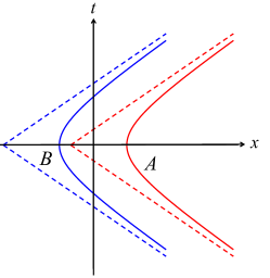
(a)

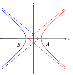
(b)

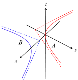
(c)

Figure 1: The worldlines of two uniformly accelerated detectors in three acceleration scenarios: the parallel acceleration (left), the anti-parallel acceleration(middle) and the perpendicular acceleration (right).

II.2.1 Parallel acceleration

Suppose that two detectors are accelerated along the $x$-direction with an acceleration $a$. The trajectories can be written as Salton-Man:2015

$$x_{A}:=\{t=a^{-1}\sinh(a\tau_{A})\;,~{}x=a^{-1}[\cosh(a\tau_{A})-1]+\frac{L}{2}\;,~{}y=z=0\}\;,$$

$$x_{B}:=\{t=a^{-1}\sinh(a\tau_{B})\;,~{}x=a^{-1}[\cosh(a\tau_{B})-1]-\frac{L}{2}\;,~{}y=z=0\}\;,$$ (8)

where $L$ represents the separation between such detectors, as measured by an inertial observer at a fixed $x$ (i.e., in the laboratory reference frame).

The Wightman function for massless scalar fields in four dimensional Minkowski spacetime is given by Birrell:1984

$$W\left(x,x^{\prime}\right)=-\frac{1}{4\pi^{2}}\frac{1}{(t-t^{\prime}-i\epsilon)^{2}-|\mathbf{x}-\mathbf{x^{\prime}}|^{2}}\;.$$ (9)

The transition probability for a uniformly accelerated detector can be derived by substituting trajectories (II.2.1) into (9) and then computing (3). After some algebraic manipulations, we arrive at Zhjl:2020 ; Zhjl:2021

$$P_{D}= \frac{\lambda^{2}a\sigma}{4\pi^{3/2}}\int_{0}^{\infty}d\tilde{s}\frac{\cos(\tilde{s}\beta)e^{-\tilde{s}^{2}\alpha}\left(\sinh^{2}\tilde{s}-\tilde{s}^{2}\right)}{\tilde{s}^{2}\sinh^{2}\tilde{s}}+\frac{\lambda^{2}}{4\pi}\left[e^{-\Omega^{2}\sigma^{2}}-\sqrt{\pi}\Omega\sigma\operatorname{Erfc}(\Omega\sigma)\right]\;,$$ (10)

where $\beta=2\Omega/a$ and $\alpha=1/(a\sigma)^{2}$.

Similarly, by substituting Eqs. (II.2.1) and (9) into Eq. (5), the nonlocal correlation term $X$, denoted here by $X_{((}$ in the parallel acceleration case, can be found to be

$$X_{((} =-\lambda^{2}\int_{-\infty}^{\infty}d\tau\int_{-\infty}^{\tau}d\tau^{\prime}\chi(\tau)\chi(\tau^{\prime})e^{-i\Omega(\tau+\tau^{\prime})}\Big{[}W\left(x_{A}(\tau^{\prime}),x_{B}(\tau)\right)+W\left(x_{B}(\tau^{\prime}),x_{A}(\tau)\right)\Big{]}$$

$$=-\lambda^{2}\int_{0}^{\infty}d\tilde{y}F(\tilde{y})\;,$$ (11)

where we have introduced two variables $\tilde{x}=\tau+\tau^{\prime}$, $\tilde{y}=\tau-\tau^{\prime}$ and an auxiliary function

$$F(\tilde{y}):=\int_{-\infty}^{\infty}d\tilde{x}e^{-\frac{\tilde{x}^{2}+\tilde{y}^{2}}{4\sigma^{2}}-i\tilde{x}\Omega}D_{((}(\tilde{x},\tilde{y})$$ (12)

with the symmetrized Wightman function $D_{((}(\tilde{x},\tilde{y})$ given by

$$D_{((}(\tilde{x},\tilde{y}):= \frac{1}{2}\Big{[}W\left(x_{A}(\tau^{\prime}),x_{B}(\tau)\right)+W\left(x_{B}(\tau^{\prime}),x_{A}(\tau)\right)\Big{]}$$

$$= \frac{a^{2}}{32\pi^{2}}\Bigg{\{}\bigg{[}\Big{(}\frac{aL}{2}-e^{-\frac{\tilde{x}a}{2}}\sinh\frac{\tilde{y}a}{2}\Big{)}\Big{(}\frac{aL}{2}+e{{}^{\frac{\tilde{x}a}{2}}}\sinh\frac{\tilde{y}a}{2}\Big{)}-i\epsilon\bigg{]}^{-1}$$

$$+\bigg{[}\Big{(}\frac{aL}{2}+e^{-\frac{\tilde{x}a}{2}}\sinh\frac{\tilde{y}a}{2}\Big{)}\Big{(}\frac{aL}{2}-e{{}^{\frac{\tilde{x}a}{2}}}\sinh\frac{\tilde{y}a}{2}\Big{)}-i\epsilon\bigg{]}^{-1}\Bigg{\}}\;.$$ (13)

In general, the double integral for $X_{((}$ can be numerically evaluated by first integrating Eq. (12) in the sense of the Cauchy principal value as long as the Wightman functions are treated as the well-defined distributions Bogolubov:1990 . Here, it is easy to see that $F(\tilde{y})$ is an even function of the detectors’ separation, so that $X_{((}$ is invariant under an exchange between detector $A$ and $B$ as expected.

II.2.2 Anti-parallel acceleration

For the anti-parallel acceleration scenario, the trajectories for two accelerated detectors can be simply written in the following form Salton-Man:2015

$$x_{A}:=\{t=a^{-1}\sinh(a\tau_{A})\;,~{}x=a^{-1}[\cosh(a\tau_{A})-1]+\frac{L}{2}\;,~{}y=z=0\}\;,$$

$$x_{B}:=\{t=a^{-1}\sinh(a\tau_{B})\;,~{}x=-a^{-1}[\cosh(a\tau_{B})-1]-\frac{L}{2}\;,~{}y=z=0\}\;,$$ (14)

where $L$ represents the separation between the detectors at their closest approach (i.e., the minimum distance at the origin of the time coordinate) as seen by a rest observer located at a constant $x$, and $a$ again stands for the magnitude of the acceleration along the $x$-axis. Here, it is worth pointing out that the nonzero $L$ in the trajectories (II.2.2) generally relaxes the condition of overlapping apexes shared by four Rindler wedges of two detectors Salton-Man:2015 . The transition probability still has the same form as Eq. (10), and the nonlocal correlation term, now denoted by $X_{)(}$ in the anti-parallel acceleration scenario, can be straightforwardly deduced by substituting Eq. (II.2.2) into Eq. (5)

$$X_{)(}=-\lambda^{2}\int_{-\infty}^{\infty}d\tilde{x}\int_{0}^{\infty}d\tilde{y}e^{-\frac{\tilde{x}^{2}+\tilde{y}^{2}}{4\sigma^{2}}-i\tilde{x}\Omega}{D_{)(}(\tilde{x},\tilde{y})}\;,$$ (15)

where

$$D_{)(}(\tilde{x},\tilde{y})= \frac{a^{2}}{16\pi^{2}}\Bigg{\{}\bigg{[}e^{-\frac{\tilde{y}a}{2}}\Big{(}\frac{La}{2}-1\Big{)}+\frac{ae^{-a\tilde{y}/2}}{2}i\epsilon+\cosh\frac{\tilde{x}a}{2}\bigg{]}\bigg{[}e^{\frac{\tilde{y}a}{2}}\Big{(}\frac{La}{2}-1\Big{)}-\frac{ae^{a\tilde{y}/2}}{2}i\epsilon+\cosh\frac{\tilde{x}a}{2}\bigg{]}\Bigg{\}}^{-1}$$

$$= \frac{a^{2}}{16\pi^{2}}\Bigg{\{}\bigg{[}e^{-\frac{\tilde{y}a}{2}}\Big{(}\frac{La}{2}-1\Big{)}+\cosh\frac{\tilde{x}a}{2}\bigg{]}\bigg{[}e^{\frac{\tilde{y}a}{2}}\Big{(}\frac{La}{2}-1\Big{)}+\cosh\frac{\tilde{x}a}{2}\bigg{]}-i\epsilon a\sinh\left(\frac{\tilde{y}a}{2}\right)\cosh\left(\frac{\tilde{x}a}{2}\right)$$

$$+\frac{a^{2}\epsilon^{2}}{4}\Bigg{\}}^{-1}\;.$$ (16)

Absorbing the positive factor $a\sinh\left(\frac{\tilde{y}a}{2}\right)\cosh\left(\frac{\tilde{x}a}{2}\right)$ into $\epsilon$ in the second line of Eq. (II.2.2) and discarding the $\epsilon$-squared term, we have

$$D_{)(}(\tilde{x},\tilde{y})=\frac{a^{2}}{16\pi^{2}}\Bigg{\{}\bigg{[}e^{-\frac{\tilde{y}a}{2}}\Big{(}\frac{La}{2}-1\Big{)}+\cosh\frac{\tilde{x}a}{2}\bigg{]}\bigg{[}e^{\frac{\tilde{y}a}{2}}\Big{(}\frac{La}{2}-1\Big{)}+\cosh\frac{\tilde{x}a}{2}\bigg{]}-i\epsilon\Bigg{\}}^{-1}\;.$$ (17)

II.2.3 Perpendicular accelerations

Regarding the perpendicular acceleration case, the spacetime trajectories of detectors can be simply written as

$$x_{A}:=\{t=a^{-1}\sinh(a\tau_{A})\;,~{}y=a^{-1}[\cosh(a\tau_{A})-1]\;,x=z=0\}\;,$$

$$x_{B}:=\{t=a^{-1}\sinh(a\tau_{B})\;,~{}x=a^{-1}[\cosh(a\tau_{B})-1]+L\;,y=z=0\}.$$ (18)

with $a$ the acceleration magnitude and $L$ the detectors’ separation at the closest approach.

Similarly, the nonlocal correlation term in the present case denoted by $X_{\perp}$ is given by

$$X_{\perp}=-{\lambda^{2}}\int_{-\infty}^{\infty}d\tilde{x}\int_{0}^{\infty}d\tilde{y}e^{-\frac{\tilde{x}^{2}+\tilde{y}^{2}}{4\sigma^{2}}-i\tilde{x}\Omega}D_{\perp}(\tilde{x},\tilde{y})$$ (19)

where

$$D_{\perp}(\tilde{x},\tilde{y})=\frac{a^{2}}{8\pi^{2}}\Big{[}\frac{1}{h_{+}(\tilde{x},\tilde{y})}+\frac{1}{h_{-}(\tilde{x},\tilde{y})}\Big{]}$$ (20)

with

$$h_{\pm}(\tilde{x},\tilde{y})= 3+(aL-1)^{2}-4\cosh(a\tilde{x}/2)\cosh(a\tilde{y}/2)-\cosh(a\tilde{y})$$

$$+\cosh(a\tilde{x})+2aL\cosh[a(\tilde{x}\pm{\tilde{y}})/2]-i\epsilon\;.$$ (21)

Although the basic formulae for entanglement harvesting are given above explicitly, exact analytic results are not easy to obtain due to the complicated double integrals. In what follows, we resort to numerical computation.

III Numerical results

In this section, we will consider how acceleration affects entanglement harvesting, first exploring the acceleration-assisted entanglement harvesting in the proposed acceleration scenarios in the sense of the entanglement harvested. We begin the discussion by plotting the concurrence as a function of the detectors’ separation $L/\sigma$ (Fig. (2)) or the acceleration $a\sigma$ (Fig. (3)) at various energy gaps $\Omega\sigma$ for all three scenarios.

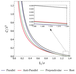
(a) $\Omega\sigma=0.01$

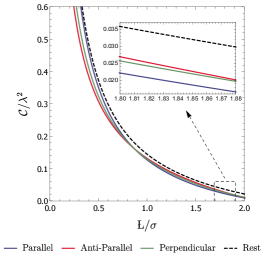
(b) $\Omega\sigma=0.50$

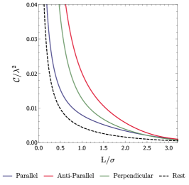
(c) $\Omega\sigma=2.00$

Figure 2: The concurrence is plotted as a function of $L/\sigma$ with fixed $a\sigma=0.50$, and $\Omega\sigma=\{0.01,0.50,2.00\}$ from left to right. Here, different colored solid lines correspond to different acceleration scenarios, and the dashed line indicates the situation of detectors at rest. For convenience, all other physical quantities are expressed in units of parameter $\sigma$.

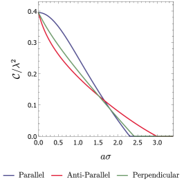
(a) $\Omega\sigma=0.01$

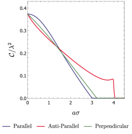
(b) $\Omega\sigma=0.50$

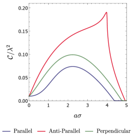
(c) $\Omega\sigma=2.00$

Figure 3: The concurrence, $\mathcal{C}(\rho_{AB})/\lambda^{2}$, is plotted as a function of $a\sigma$ for various energy gaps $\Omega\sigma=\{0.01,0.50,2.00\}$ with $L/\sigma=0.50$. In the limit of $a\sigma\rightarrow 0$, the concurrence $\mathcal{C}(\rho_{AB})$ approaches the corresponding value for detectors at rest in Minkowski spacetime.

For a small energy gap ($\Omega\sigma<1$), we find that the harvested entanglement generally degrades with increasing acceleration and with increasing detector separation. As a consequence, inertial detectors (at rest) harvest more entanglement. In this sense, acceleration suppresses entanglement harvesting due to the strong thermal noise associated with the Unruh effect. Similar results have also been found for accelerated detectors in four-dimensional Minkowski spacetime with a reflecting boundary Zhjl:2021 .

Upon closer inspection, some interesting features emerge. A cross-comparison of the concurrences for small accelerations, small separations, and small gaps, indicates that the parallel scenario harvests comparatively more entanglement than the perpendicular one, which in turn harvests more than the antiparallel case. However we see that the parallel case has the most rapid decrease and so a crossover effect occurs for both sufficiently large separation and acceleration, with the rank-ordering reversed: antiparallel harvesting the most and parallel the least. The point of crossover is gap-dependent, as is clear upon comparison of the left diagrams with the middle ones in Fig.(2a)&(2b) or Fig.(3a)&(3b)). Similar effects were reported in Ref. Zhjl:2021 .

For sufficiently large gaps ($\Omega>L/\sigma^{2}$ and $\Omega>a$) the thermal noise caused by acceleration ceases to play a significant role in entanglement harvesting. As shown in Fig. (3c), concurrence is no longer a monotonically decreasing function of acceleration. In fact, for small $a\sigma$, the concurrence is instead a monotonically increasing function of $a\sigma$, meaning that the detectors in all three acceleration scenarios are likely to harvest more entanglement from the fields than the detectors at rest. This is in sharp contrast to the aforementioned results for a small energy gap. The concurrence maximizes in all scenarios at some intermediate value of the acceleration, peaking most strongly in the antiparallel scenario, with the parallel scenario harvesting the smallest amount throughout.

Notably interesting features appear in Fig. (2c), which plots concurrence against separation for a large gap. We see the rank-ordering from smallest to largest is parallel to perpendicular to antiparallel, as in Fig. (3c), but with the remarkable feature that all three scenarios harvest more entanglement than the situation where the detectors are at rest. As separation increases, concurrence decreases, with the curves tending to merge at large $L$.

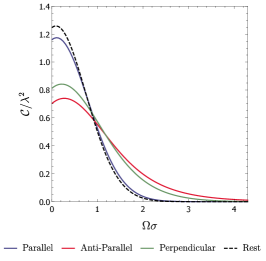
(a) $L/\sigma=0.20$

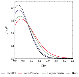
(b) $L/\sigma=0.50$

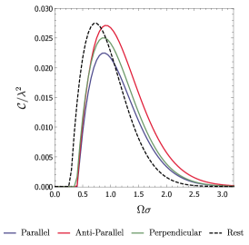
(c) $L/\sigma=2.00$

Figure 4: The concurrence is plotted as the function of $\Omega\sigma$ with $a\sigma=0.50$ and $L/\sigma=\{0.20,0.50,2.00\}$ in left-to-right order. The dashed line indicates the detectors is at rest.

To gain a better understanding of the influence of the energy gap, we plot concurrence as a function of $\Omega\sigma$ for all acceleration scenarios in Fig. (4). For small separations $L/\sigma\lesssim 1$, concurrence grows with increasing $\Omega\sigma$, reaching a maximum at some $\Omega\sigma<1$ in each scenario, the ascending rank-ordering being antiparallel to perpendicular to parallel, with the rest case harvesting the largest amount of entanglement. However once $\Omega\sigma>1$ the situation dramatically changes: the rank-ordering is reversed, with inertial detectors (at rest) harvesting the least amount of entanglement.

For large separations, we see from Fig. (4c) that the situation changes yet again. There is a peak in the concurrence at some value of $\Omega\sigma$ for all acceleration scenarios, with the parallel to perpendicular to antiparallel ordering from lowest to highest concurrence holding over almost the entire gap range. But the inertial scenario differs from these: it is larger than the acceleration scenarios for a small $\Omega\sigma$, but peaks earlier, and is subsequently overtaken by the other cases.

Similar peaking behavior of the concurrence has also been discovered in some spacetimes with nontrivial topologies Zhjl:2018 ; Zhjl:2019 ; Robbins:2020jca . Indeed, the value of the peak is strongly dependent on $L/\sigma$, and the larger the detectors’ separation, the smaller the peak value.

We again find a contrast with Ref. Salton-Man:2015 , where it was argued that there is an effect of entanglement resonance in the anti-parallel acceleration scenario with the energy gap being $\Omega_{\rm{res}}=\arccos[(2-aL)/2]/(a\sigma^{2})$ for any $aL<4$, which would render the nonlocal correlation term $X$ divergent, resulting in an infinite concurrence ${\cal{C}}(\rho_{AB})$. Our numerical integrations clearly show that all corresponding quantities are finite and regular, even at point $\Omega=\Omega_{\rm{res}}$ (see Fig. (4)). This discrepancy is due to the manner of computing the integrals, which should be carried out in terms of the Cauchy principal value rather than under a saddle point approximation as in Salton-Man:2015 . We conclude that there is no resonance effect associated with an infinite concurrence in the anti-parallel acceleration scenario.

We now turn to explore the harvesting-achievable separation range between the detectors in all three scenarios. For convenience, we introduce a parameter, $L_{\rm{max}}$, to characterize the maximum harvesting-achievable range, beyond which entanglement harvesting cannot occur. As shown in Fig. (5), it is easy to see that $L_{\rm{max}}$ is a predominantly increasing function of the energy gap.

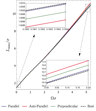
(a) $a\sigma=0.01$

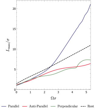
(b) $a\sigma=1.00$

Figure 5: The maximum harvesting-achievable separation between two detectors versus the energy gap. Here, we have set $a\sigma=\{0.01\;,1.00\}$ from left-to-right, and the dashed curve denotes the case of detectors at rest.

For a very small acceleration ($a\sigma\ll 1$), the inertial case has the largest harvesting-achievable range in the small gap regime, followed by parallel, perpendicular, and antiparallel. This rank ordering tends to converge as the gap increases, and then reverses order for a sufficiently large gap, as shown in Fig. (5a)). The anti-parallel acceleration scenario then becomes the optimum choice that has most “room” to accessibly harvest entanglement.

More interestingly, we see in Fig. (5b) that for a large, but not too large $a\sigma$, the parallel acceleration case possesses the largest $L_{\rm{max}}$, exceeding that of the inertial detector when $\Omega\sigma\gg\ 1$ and $\Omega>a$. By contrast, the harvesting-achievable range for the anti-parallel and perpendicular scenarios cannot exceed that of the inertial case.

Summarizing, we find that enhancement of entanglement harvesting happens not only in the anti-parallel scenario, but also in the parallel and perpendicular acceleration cases, in sharp contrast to what was argued previously Salton-Man:2015 , namely that there is an enhancement only compared to inertial motion only in the anti-parallel scenario. Moreover, the harvesting-achievable range of acceleration-assisted enhancement is not universal, holding only for sufficiently large energy gaps ($\Omega\sigma\gg 1$) in the parallel acceleration case, and for sufficiently large energy gaps with small accelerations ($a\sigma\ll 1$) also in the anti-parallel and perpendicular cases.

IV conclusion and summary

In the framework of the entanglement harvesting protocol, we performed a complete study on acceleration assisted entanglement harvesting for two uniformly accelerated detectors in three different scenarios: parallel, anti-parallel and mutually perpendicular accelerations. We considered both the amount of entanglement harvested and the maximal harvesting-achievable separation between the two detectors. Our numerical evaluation of the integrals involved in the analysis was carried out in terms of the Cauchy principal value, treating the Wightman function as a distribution rather than using a saddle point approximation as in Salton-Man:2015 .

Regarding the amount of harvested entanglement, we find that the detectors at rest with small energy gaps $\Omega\sigma<1$ harvest comparatively more entanglement than accelerating ones, suggesting that no acceleration-assisted entanglement harvesting occurs here. In terms of the amount of concurrence harvested, the rank-ordering from largest to smallest is parallel/perpendicular/anti-parallel for small gaps and separations. For sufficiently large values of these parameters, this rank-ordering is inverted. Furthermore, and quite surprisingly, acceleration can increase the amount of entanglement harvested for all three acceleration scenarios once the energy gap is sufficiently large. There exists a peak in the concurrence at certain positive energy gap. We find no evidence for entanglement resonance, as argued in Salton-Man:2015 .

As for the harvesting-achievable separation range, we find that acceleration hinders entanglement harvesting for detectors with a very small gap $\Omega\sigma\ll 1$, with inertial detectors (at rest) possessing a relatively larger harvesting-achievable range. However, for a large enough $\Omega\sigma$ and a small acceleration, accelerated detectors in all scenarios possess a comparatively larger harvesting-achievable range than detectors at rest – acceleration now assists entanglement. Especially for a not too small acceleration, the parallel scenario with the gap larger than the acceleration has the largest harvesting-achievable range amongst all scenarios, exceeding that of the inertial case. The anti-parallel and perpendicular scenarios, however, are unable to overtake the inertial case in terms of their harvesting-achievable range. These results are in sharp contrast to the previous claim Salton-Man:2015 , that enhancement of the harvesting-achievable range occurs only in the anti-parallel acceleration scenario.

Based on the arguments presented here, a natural question worthy of future study that emerges from considerations of the equivalence principle is the extent to which spacetime curvature can assist entanglement harvesting. Some investigations in this regard in AdS spacetime Zhjl:2019 ; Ng:2018-2 and for BTZ black holes Zhjl:2018 ; Robbins:2020jca have shown that curvature can have significant effects on this process. However relatively little is known about $(3+1)$ (and higher)-dimensional cases, which merit detailed exploration. It is also worthwhile to go beyond the massless scalar field case considered here to the massive one and to other quantum fields.

- (1) W. G. Unruh, Phys. Rev. D 14, 870 (1976).
- (2) L. C. B. Crispino, A. Higuchi, G. E. A. Matsas, Rev. Mod. Phys. 80, 787 (2008).
- (3) S.W. Hawking, Comm. Math. Phys. 43, 199 (1975).
- (4) G.W. Gibbons and S.W. Hawking,Phys. Rev. D 15, 2738 (1977).
- (5) E. Martin-Martinez, I. Fuentes, Robert B. Mann, Phys. Rev. Lett. 107, 131301(2011).
- (6) J. Hu, H. Yu, Phys. Rev. A 85, 032105 (2012).
- (7) H. Zhai, J. Zhang and H. Yu, Ann. Phys. (N. Y.) 371, 338 (2016).
- (8) J. Audretsch and R. Müller, Phys. Rev. A 52, 629 (1995).
- (9) R. Passante, Phys. Rev. A 57,1590 (1998).
- (10) Z. Zhu and H. Yu, Phys. Rev. A 82, 042108 (2010).
- (11) F. Benatti and R. Floreanini, Phys. Rev.A 70, 012112 (2004).
- (12) I. Fuentes-Schuller and R. B. Mann, Phys. Rev. Lett. 95, 120404 (2005).
- (13) P. M. Alsing, I. Fuentes-Schuller, R. B. Mann and T. E. Tessier, Phys. Rev. A 74, 032326 (2006).
- (14) J. Zhang and H. Yu, Phys. Rev. D 75, 104014 (2007).
- (15) A. G. S. Landulfo and G. E. A. Matsas, Phys. Rev. A 80, 032315 (2009).
- (16) J. Doukas and B. Carson, Phys. Rev. A 81, 062320 (2010).
- (17) D. C. M. Ostapchuk, S.-Y. Lin, R. B. Mann and B. L. Hu, J. High Energy Phys.07(2012) 072.
- (18) J. Hu and H. Yu, Phys.Rev. A 91, 012327 (2015).
- (19) S. Cheng, H. Yu and J. Hu, Phys. Rev. D 98, 025001 (2018).
- (20) J. I. Koga, K. Maeda, G. Kimura, Phys. Rev. D 100, 065013 (2019).
- (21) J. She, J. Hu, H. Yu, Phys. Rev. D 99, 105009 (2019).
- (22) J. Zhang and H. Yu, Phys. Rev. D 102, 065013 (2020).
- (23) D. Barman, S. Barman, B. R. Majhi, J. High Energy Phys. 07(2021)124; P. Chowdhury, B. R. Majhi, arXiv:2110.11260 [hep-th].
- (24) S. J. Summers and R. Werner,J. Math. Phys. (N.Y.) 28, 2448 (1987).
- (25) A. Valentini, Phys. Lett. A 91,153321 (1991).
- (26) B. Reznik, Foundations of Physics 33,167 (2003); B. Reznik, A. Retzker, and J. Silman, Phys. Rev. A 71, 042104 (2005).
- (27) G. Salton, R.B. Mann and N.C. Menicucci, New J. Phys 17, 035001 (2015).
- (28) A. Pozas-Kerstjens and E. Martin-Martinez, Phys. Rev. D 92, 064042 (2015).
- (29) W. Cong, E. Tjoa and R.B. Mann, J. High Energy Phys. 06 (2019) 021.
- (30) W. Cong, C. Qian, M. R. R. Good and R. B. Mann, J. High Energy Phys. 10(2020) 067.
- (31) Z. Liu, J. Zhang and H. Yu, J. High Energy Phys.08(2021) 020.
- (32) E. Martin-Martinez, A. R. H. Smith and D. R. Terno, Phys. Rev. D 93, 044001 (2016).
- (33) G. L. Ver Steeg and N. C. Menicucci, Phys. Rev. D 79, 044027 (2009).
- (34) Y. Nambu, Entropy 15, 1847 (2013).
- (35) S. Kukita and Y. Nambu, Entropy 19, 449(2017).
- (36) L. J. Henderson, R. A. Hennigar, R. B. Mann, A. R. H. Smith and J. Zhang, J. High Energy Phys.05 (2019) 178 .
- (37) M. P. G. Robbins, L. J. Henderson and R. B. Mann, Classical Quantum Gravity 39, 02LT01 (2022).
- (38) K. K. Ng, R. B. Mann and E. Martin-Martinez, Phys. Rev. D 98,125005 (2018).
- (39) L. J. Henderson, R. A. Hennigar, R.B. Mann, A. R H. Smith and J. Zhang, Class. Quant. Grav. 35, 21LT02 (2018).
- (40) L. J. Henderson, A. Belenchia, E. Castro-Ruiz, C. Budroni, M. Zych, Č. Brukner and R. B. Mann, Phys. Rev. Lett. 125, no.13, 131602 (2020).
- (41) E. Tjoa and R. B. Mann, J. High Energy Phys. 08 (2020) 155.
- (42) K. Gallock-Yoshimura, E. Tjoa, Robert B. Mann,Phys. Rev. D 104, 025001 (2021).
- (43) N. D. Birrell and P. C. W. Davies, Quantum Fields in Curved Space(Cambridge University Press, Cambridge, U.K.,1984).
- (44) N. N. Bogolubov, A. A. Logunov, A. I. Oksak and I. T. Todorov, General Principles of Quantum Field Theory (Kluwer Acaciemic Publishers, Dordrecht, The Netherlands, 1990).