A Quantum Field Theoretical Study of Correlated Quantum Ising model with Longer Range Interaction

Abstract

The physics of quantum Ising model (qIm) plays an important role in quantum many body system. We study and present the results of qIm and longer range quantum Ising model (lqIm) in presence of strong correlation. We do the quantum field theoretical renormalization group (RG) calculation to study the behaviour of RG flow lines for different couplings for different region of parameter space. We show how the strong correlation effect enrich the quantum physics of these two systems. We show explicitly that the ordered ferromagnetic (FM) phase to the disorder quantum paramagnet (dqpI) quantum phase transition occurs for only in the strongly correlated regime for qIm and the dqpI phase appears for non-interacting and attractive regime. We show explicitly for lqIm that FM to dqpI transition occurs at the extremely correlated region and also the dqpI phase appears in correlated regime. We show that short range FM coupling and longer range coupling are competiting with each other and also the effect of strong correlation in this competition. We also show the most interesting feature that the transverse field oppose the FM coupling of qIm but it is favour the longer range coupling of lqIm. We find the evidence of another disorder quantum paramagnetic (dqpII) phase due to the relevance of longer range coupling. We also present the existence of another quantum phase transition from dqpII phase to FM phase. We show explicitly that there is no phase transition from dqpI phase to dqpII phase rather they coexists. This work provides a new perspective not only for the statistical physics of quantum Ising model but also for the quantum many body systems.

1 Introduction

The physics of quantum Ising model (qIm) plays an important role in one dimensional quantum many body system ^1-8. The physics of one dimensional quantum many body is interesting in its own right ^9,10. One dimensional quantum many body system has strong quantum fluctuations that do not allow spontaneously broken continuous symmetries As a result of this, the pairing instabilities do not lead to any ordered density-wave ^11,12. This many body has a critical phase with power law decay of various correlation functions, universally known as a Luttinger liquid. In one dimensional quantum many body systems whether it is weakly correlated or strongly proper treatment of the quantum fluctuations leads in both cases to a Luttinger liquid characterized by phonon-like collective density fluctuation modes. In this process there is a one-to-one correspondence between excitations of a one dimensional free Fermi gas and free bosons. This can be used to solve the strongly interacting fermion problem by turning it into a weakly interacting boson problem via the method of bosonization followed by the quantum field theoretical renormalization group study ^13-16. In the present study, we use the bosonization process to recast the model Hamiltonian in continuum field theory followed by the renormalization group (RG) method.
It is well known that the Coulomb interaction is always present in the solid state, either screened or weak or sometimes even stronger. Coulomb interaction leads to the different physical phenomena in quantum many-body systems, such as the Kondo effect, Mott-Hubbard transition and superconductivity to mention a few ^9,10. Therefore, to get a complete picture of emergent quantum phases of a quantum many-body system, one has to consider the effect of correlation ^9,10. In the correlated many-body system, this situation is described by the celebrated sine-Gordon model ⁹, which also plays a central role in quantum field theory. In the low energy limit, effective degrees of freedom give the accurate description of the system . It is one of the method by which one find the low energy effective theory.
The mathematical structure and results of the RG theory are a significant conceptual advancement in quantum field theory in the last several decades in both high-energy and quantum many body condensed matter physics. The need for RG is really transparent in condensed matter physics. RG theory is a formalism that relates the physics at different length scales in condensed matter physics and the physics at different energy scales in high-energy physics ^17,18. We focus on systems that can be mapped to a dual-field double sine-Gordon model as a bosonized effective field theory. In this study we do the quantum field theoretical RG calculation for the correlated quantum Ising model (qIm) and longer range quantum Ising model (lqIm). We want to study this problem from the perspective of one dimensional correlated quantum many body system.
Motivation of this study
The physics of qIm has already studied extensively in the literature ^1-7. But still the physics of strong correlation has not explored for qIm. The quantum field theoretical study of our model Hamiltonian has not explored in the literature, specially how the strong correlation physics explore for this model Hamiltonian. In the literature quite a few studies have already been done for this model Hamiltonian from the perspective of topological state. But the main motivation of our study is to explore the physics from the perspective of correlated quantum many body system. This model Hamiltonian has three competiting interaction terms, the most interesting feature of this study is to show how the behaviour of RG flow lines reflect for these three competiting interaction and finally leads to emergence phase.

2 Model Hamiltonian and Renormalization Group Equation:

The model Hamiltonian¹⁹ of the present study is

$$H=-\sum_{i}(\mu{{\sigma}_{i}}^{x}+{\lambda}_{1}{{\sigma}_{i}}^{z}{{\sigma}_{i+1}}^{z}+{\lambda_{2}}{{\sigma}_{i}}^{x}{\sigma_{i-1}}^{z}{\sigma_{i+1}}^{z}).$$ (1)

Here $\mu$ is the chemical potential, $\lambda_{1}$ is the two spin interaction of nearest-neighbour (NN) sites and $\lambda_{2}$ is the three spin interactions. Thus we term this model Hamiltonian as lqIm with three spin interaction.
It is well known to us for qIm, the system is in disorder quantum phase when the transverse field exceed the FM coupling, we term this disorder quantum phase as dqpI. The coupling $\lambda_{2}$ is related with the three sites (i-1, i and i+1 ), the left (i-1) and right (i+1 ) sites are related with the $\sigma_{z}$ operator and the middle site (i) is with the $\sigma_{x}$ operator $\sigma_{x}$ operator. It is very clear from this interaction term that next-nearest-neighbour (NNN) sites are related with the FM interaction but NN sites are related with the $XZ$ interaction, i.e, the spin flipping occurs at the site i. This interaction introduce the frustration in the system and finally leads to the disorder quantum phase. We term this disorder quantum phase as dqpII. We will see after the derivation of quantum field theoretical RG equations that the behaviour of the RG flow lines for the couplings $\mu$ and $\lambda_{2}$ are the same and this result is also supported from the study of scaling relation. Thus in this quantum many body system possesses two different kind of disorder quantum phases.
The whole Hamiltonian (eq.1) have been also studied previously in different contexts The model was first introduced by the authors of Ref. 19 to study the persistence of quantum criticality at high temperature in correlated systems. The authors of Ref.20 have studied the physics of Majorana zero modes in the gapped phases of this model with both broken and unbroken time-reversal symmetry. One of the authors (S.S) has studied the quantization of geometric phase with integer and fractional topological characterization for this model in Ref.21. Very recently authors of Ref.22 have solved the problem of bulk-boundary correspondence at the quantum critical lines and discussed the principle of least topological invariant number at the criticality. The author Ref. 23 have also studied Curvature RG of this model Hamiltonian. But the quantum field theoretical RG study and the interpretation of emergent quantum phases from the perspective of quantum many body physics is absent in the literature.

The model Hamiltonian can be described by the sine-Gordon field theory as,

$$H=H_{0}+V(\phi,\theta),$$ (2)

where $H_{0}$ is

$$H_{0}=(\frac{{h}v}{2\pi})\int dx[{({\partial_{x}\theta(x)})}^{2}+{({\partial_{x}\phi(x)})}^{2}].$$ (3)

The Hamiltonian, $H_{0}$ gives a universal framework for describing one dimensional interacting bosons and fermionic system, i.e., Tomonoga-Luttinger liquid (TLL) Hamiltonian and $V(\phi)$ is the sine-Gordon potential. $\theta(x)$ is the dual field of $\phi(x)$ and satisfy the following commutation relation , $[\phi(x),\partial_{x}\theta(x^{\prime})]=-i\pi\delta(x-x^{\prime})$. $v$ is the velocity of the collective excitation of the system. We write final form of Bosonized Hamiltonian as (detail derivation is relegated to to the "Method" section),

$$V(\phi,\theta)=\frac{\lambda_{1}}{2}\int\cos[4\sqrt{\pi K}\phi(x)]dx-\mu\int\cos[2\sqrt{\pi K}\phi(x)]\cos[\sqrt{\frac{\pi}{K}}\theta(x)]dx\\ -\frac{\lambda_{2}}{\pi}\int\cos[2\sqrt{\pi K}\phi(x)]\cos[\sqrt{\frac{\pi}{K}}\theta(x)]\left(\partial_{x}\sqrt{K}\phi(x)\right)^{2}dx$$ (4)

The bosonized form of the model Hamiltonian consists four terms. The first term is the kinetic energy term and the rest three terms present the sine-Gordon coupling terms. It is to be noted that the starting Hamiltonian (eq. 1) has no $K$, term but it appears after the continuum field theoretical calculation in the bosonized version of the Hamiltonian (detail derivation is relegated to the "Method" section). $K$ is the Tomonoga-Luttinger liquid (TLL) parameter to present the interaction strength in the system. The physics of low-dimensional quantum many body condensed matter system is enriched with its new and interesting emergent behavior. $K<1$ and $K>1$ and $K=1$ characterizes the repulsive, attractive interactions and non-interacting, respectively ^9,24,25.
We notice that the nearest-neighbour (NN) coupling term ($\lambda_{1}$) is related with the a single sine-Gordon coupling term of the field ($\phi$ (x) ). The transverse field is the product of two sine-Gordon coupling terms of $\phi(x)$ and $\theta(x)$ which are dual to the each other. But we notice that for the longer range coupling with three spin interaction is also product of two sine-Gordon coupling terms augmented with a part of the kinetic energy term from the field $\phi(x)$. These extra two sine-Gordon coupling terms for the longer range interaction over the quantum Ising model give the enrich quantum physics over the qIm.
It is very clear from the continuum field theoretical study that our model Hamiltonian contains three strongly relevant and mutually nonlocal perturbations over the Gaussian (critical) theory. In such a situation, the strong coupling fixed point is usually determined by the most relevant perturbation whose amplitude grows up according to its Gaussian scaling dimensions and it is not much affected by the less relevant coupling terms. However, this is not the general rule if the operators exclude each other. In this case, the interplay between the three competing relevant operators (here $\mu$, $\lambda_{1}$ and $\lambda_{2}$) are the three competing relevant operators, which are related with dual fields $\theta(x)$ and $\phi(x)$ can produce a novel quantum phase transition through a critical point or a critical line ^24,25. Therefore, the present study based on RG equations will give us the appropriate results for these model Hamiltonian.

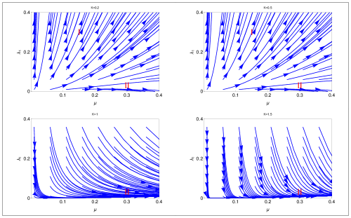
Figure 1: (Color online.) This figure shows the behaviour of renormalization group flow lines for the couplings $\lambda_{1}$ and $\mu$ (eq. 5) for the different initial values of $K$ as depicted in figures.

Now we present the RG equations for the present study:
(1). The RG equation for the correlated qIm is the following (detail derivation is related to the "Method" section ),

$$\frac{d\lambda_{1}}{dl} =(2-4K)\lambda_{1}+\frac{\mu^{2}}{8}(2K-\frac{1}{2K})$$

$$\frac{d\mu}{dl} =(2-K-\frac{1}{4K})\mu+\lambda_{1}\mu K$$

$$\frac{dK}{dl} =-\lambda_{1}^{2}K^{2}$$ (5)

(2). The RG equation for the correlated lqIm is the following, (detail derivation is related to the "Method" section ),

$$\frac{d\lambda_{1}}{dl} =(2-4K)\lambda_{1}+\frac{\mu^{2}}{8}(2K-\frac{1}{2K})$$

$$\frac{d\lambda_{2}}{dl} =(2-K-\frac{1}{4K})\lambda_{2}+\frac{\lambda_{1}\lambda_{2}K}{\pi}$$

$$\frac{d\mu}{dl} =(2-K-\frac{1}{4K})\mu+\lambda_{1}\mu K$$

$$\frac{dK}{dl} =-\lambda_{1}^{2}K^{2}$$ (6)

(3). RG equation for the correlated lqIm without transverse field ($\mu=0$).
(detail derivation is related to the "Method" section ),

$$\frac{d\lambda_{1}}{dl} =(2-4K)\lambda_{1}$$

$$\frac{d\lambda_{2}}{dl} =(2-K-\frac{1}{4K})\lambda_{2}+\frac{\lambda_{1}\lambda_{2}K}{\pi}$$

$$\frac{dK}{dl} =-\lambda_{1}^{2}K^{2}$$ (7)

The most interesting feature of these three set of RG equations is the appearance of K, therefore the behaviour of the RG flow lines will be affected by the strong correlation.

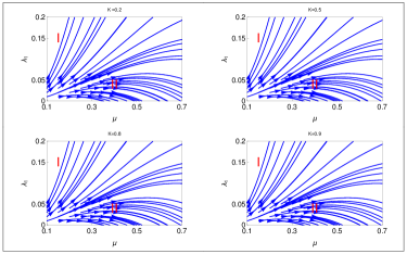
Figure 2: (Color online.) This figure shows the behaviour of renormalization group flow lines for the couplings $\lambda_{1}$ and $\mu$ (eq. 5) for the different initial values of $K$ as depicted in figures.

3 Results:

(A). Effect of strong correlation in quantum Ising model
Fig. 1, presents the RG flow diagrams for the couplings $\lambda_{1}$ and $\mu$ from the study of RG flow equation (eq. 5). It consists of four figures for different values of $K$ as depicted in the figures. The figures for the first panel are for strongly correlated regime , i.e., the $K<1$. The most interesting feature that we observe from these behavior of RG flow lines is that there is a transition from the ordered FM phase to dqpI phase. The behaviour of RG flow lines are the same for the entire correlated regime. It reveals from this study that both the coupling $\lambda_{1}$ and $\mu$ are flowing off to the strong coupling phase but the coupling $\lambda_{1}$ increases more sharply than the smaller initial values of $\mu$. But it reveals from the behaviour of RG flow lines for smaller initial values of $\lambda_{1}$ the RG flow lines are flowing off to the weak coupling phase finally touches the base line, i.e., the system is in the dqpI phase, we term this phase as dqpI. We find the quantum phase transition from the ordered FM phase to dqpI phase to search this quantum phase transition in the repulsive regime of strongly correlated phase. Thus we bench mark the standard results of qIm of literature ^1-7.
In fig.2 we show it explicitly from perspective of correlated physics.
The lower panel presents the results for non-interacting ($K=1$) and attractive regime ($K>1$). The behaviour of the RG flow lines for the coupling, $\lambda_{1}$ is flowing off to the weak coupling phase and finally touch the base line. For this situation system is in the dqpI phase. For these two figures, we have not found any quantum phase transition between the order FM phase to dqp phase. The RG flow lines are much more stiffer for the attractive regime of the parameter space.

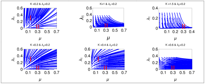
Figure 3: (Color online.) This figure shows the behaviour of renormalization group flow lines for the couplings $\lambda_{1}$ and $\mu$ (eq. 6) for the different initial values of $K$ and $\lambda_{2}$ as depicted in the figure.

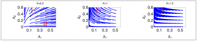
Figure 4: (Color online.) This figure show the behaviour of renormalization group flow lines for the couplings $\lambda_{2}$ and $\lambda_{1}$ (eq. 7) for the different initial values of $K$ as depicted in figures.

Fig. 2, presents the RG flow diagrams for the couplings $\lambda_{1}$ and $\mu$ from the study of qIm (eq. 5). It consists of four figures for different values of $K$ as depicted in the figures. The all figures are for strongly correlated regime , i.e., the $K<1$. The main theme of this figure is to show the evidence of order FM to dqp phase transition explicitly. The region (I) is the order FM phase and region (II) is the dqpI phase, the behaviour of the RG flow lines are the same for the all initial values of $K$ in the correlated regime. One of the hall-mark of this study is that only quantum phase transition occurs in the strongly correlated regime ,i.e., there is no evidence quantum phase transition for the non-interacting and attractive regime. Thus it is clear from this study that for the higher values of $K$, system prefer to stay in the dqpI phase. Now the prime task is to find the effect of longer range interaction on the qIm RG flow study.

(B). Effect of strong correlation in longer range quantum Ising model
In fig.3, we present the RG flow lines behaviour from the study of coupling $\lambda_{1}$ and $\mu$ for the RG equation (eq. 7). This figure consists of two panels, for all panels one we fix the initial value of ,$\lambda_{2}=0.2$, but for the different initial values of $K$. In the upper panel, there are three figures. The left, middle and right figures are respectively for the initial values of $K=0.2$, $1$ and $1.5$. But in the lower panel we vary the initial value of $K$ for only the correlated regime as depicted in the figures, to search the effect of $\lambda_{2}$ on the quantum phase transition. The most interesting result we obtain from the behaviour of RG flow lines for the left figures of upper and lower panel that the quantum phase transition occurs at the extremely correlated regions, i.e., for the very lower values of $K$ otherwise system is in the dqpI phase. It reveals from the behaviour of RG flow lines for the middle and right figure of the upper panel that the RG flow lines flowing off to the weak coupling phase much sharper for the higher initial values of $K$.
In the lower panel, the behaviour of RG flow lines for the right figures show that the RG flow lines are flowing off to the weak coupling phase very slowly but not touching the base line. Here there is no evidence of quantum phase transition, system is only in the order FM phase due to the relevant of coupling $\lambda_{1}$. The middle figure shows that order FM phase in region I and the existence of flat phase, i.e., the RG flow lines move with the same initial velocity in region II.
The most interesting result which we have obtained from this study that the presence of $\lambda_{2}$ drives the dqpI phase at the strongly correlated regime. The competition between the FM coupling of qIm and long range coupling favour the transverse field and drives the system to the dqpI phase at the extremely correlated regime. But for the left and middle figure we are unable to find the sharp quantum phase transition from order FM phase to dqpI phase. For the smaller values of $\lambda_{1}$, the behaviour of RG flow lines are almost flat for the middle figure.

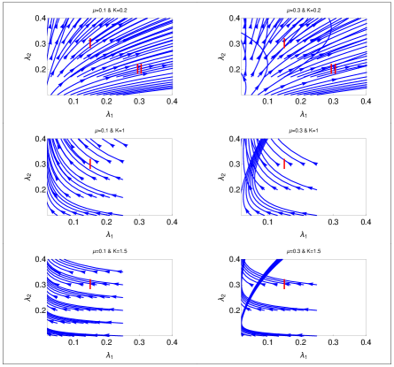
Figure 5: (Color online.) Shows the behaviour of renormalization group flow lines for the couplings $\lambda_{2}$ and $\lambda_{1}$ for the different initial values of $K$ and $\mu$. This figure consists of three rows for different initial values of $K$. We present the RG flow lines based on eq.6. The left and right figures are respectively for $\mu=0.1$ and $\mu=0.3$.

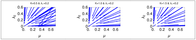
Figure 6: (Color online.) This figure shows the behaviour of renormalization group flow lines for the couplings $\lambda_{2}$ and $\mu$ (eq. 7) for the different initial values of $K$ and $\lambda_{1}$ as depicted in figures.

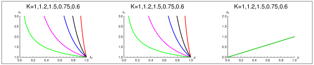
Figure 7: (Color online.) Shows the results for scaling analysis based on the equations (8) and (11). The Green, Magenta, Blue, Black and Red lines are respectively for $K=0.6,0.75,1,1.2$ and $1.5$.

Fig. 4 presents the RG flow diagrams for the couplings $\lambda_{2}$ and $\lambda_{1}$ from the study of qIm (eq. 7) in absence of transverse field. It consists of three figures for different values of $K$ as depicted in the figures. The left, middle and right figures are respectively for the strongly correlated, non-interacting and attractive regime. It give us only how the $\lambda_{1}$ and $\lambda_{2}$ compete with each other in absence of transverse field. It reveals from the behaviour of RG flow lines that for the correlated regime both of the couplings are flowing off to the strong coupling phase, but when the initial values of $\lambda_{1}$ is greater than $\lambda_{2}$, the RG flow lines for $\lambda_{1}$ flowing off more sharply than $\lambda_{2}$, i.e., the system is in the ordered FM phase for $\lambda_{1}$ coupling otherwise the system is in disorder quantum phase due to $\lambda_{2}$ coupling. The middle and right figures show that the coupling, $\lambda_{2}$, flowing off to the strong coupling phase and the system is in the disorder quantum phase due to the $\lambda_{2}$ coupling. The origin of this disorder quantum phase is entirely different from the dqpI phase from the qIm, we term this dqp phase as dqpII.
Fig. 5 presents the RG flow diagrams for the couplings $\lambda_{2}$ and $\lambda_{1}$ from the study of lqIm (eq. 6). Here we study the effect of transverse field on the RG flow lines of fig.4. This figure consists of three panels the upper, middle and lower panels are respectively for correlated ($K=0.2$), non-interacting ($K=1$) and attractive regime ($K=1.5$). Each panel consists of two figures for two different values of $\mu$, the left and right figures for each panel are respectively for $\mu=0.1$ and $0.3$.
It reveals from the RG flow lines that for higher initial values of $\lambda_{2}$, i.e, when the initial values of $\lambda_{2}>\lambda_{1}>$, the RG flow lines for the coupling $\lambda_{2}$ increase more sharply than the coupling $\lambda_{1}$ then the system is in dqpII phase. The situation is different when the initial values of $\lambda_{1}>\lambda_{2}$, for this case system is in the FM phase due to the $\lambda_{1}$ coupling, qualitative behaviour of the RG flow lines are the same. In the middle and lower panel, we observe that the RG flow lines are flowing off to the strong coupling phase due to the coupling $\lambda_{2}$, it increases very sharply for the higher values of $\mu$. Thus we finally conclude that the presence of $\mu$ help the coupling $\lambda_{2}$ flowing off to the strong coupling phase, i.e., the system is in strong coupling phase.
Fig. 6 shows the RG flow diagrams for the couplings $\lambda_{2}$ and $\mu$ from the study of qIm (eq. 7). This figure panel consists of three figures for different values of $K$ as depicted in the figures, here we fix $\lambda_{1}=0.2$. The main theme of this study is to show whether there is any competition between the $\mu$ and $\lambda_{2}$. The analytical expressions for the RG equations for these two couplings are the same at the one loop level but it differs in the second loop level. It reveals from the behaviour of RG flow lines that both of the couplings are flowing off to the strong coupling phase almost at the same speed. Thus it is clear that there is no quantum phase transition and both dqpI and dqpII phases coexist. We have already explained that the nature of coupling $\lambda_{2}$ is disorder quantum frustrated due to the three sites structure of the interaction.
We observe from these study that dqpI phase exist only for the qIm and lqIm model when we find the competition between the order FM to disorder quantum paramagnetic phase. The dqpII phase exists only for lqIm when we study the RG flow lines for the couplings $\lambda_{2}$ with $\lambda_{1}$. The effect of strong correlation is the same for the both qIm and lqIm, as we notice that the system prefers to stay in dqpI phase for the higher values of $K$.

4 Scaling Analysis:

It is well known that the critical theory is invariant under the rescaling. Then the singular part of the free energy density satisfies the following scaling relations ¹.

$$f_{s}[\mu,\lambda_{1},\lambda_{2}]={\lambda_{1}}^{2/(2-4K)}f_{s}[1,{\lambda_{1}}^{-(2-4K)/(2-K-1/4K)}\lambda_{2},{\lambda_{1}}^{-(2-4K)/(2-K-1/4K)}\mu]$$ (8)

The scaling equation for $\lambda_{1}$ and $\lambda_{2}$ is the following:

$$f_{s}[\lambda_{1},\lambda_{2}]={\lambda_{1}}^{2/(2-4K)}f_{s}[1,{\lambda_{1}}^{-(2-4K)/(2-K-1/4K)}\lambda_{2}]$$ (9)

The scaling equation for $\lambda_{1}$ and $\mu$ is the following:

$$f_{s}[\lambda_{1},\mu]={\lambda_{1}}^{2/(2-4K)}f_{s}[1,{\lambda_{1}}^{-(2-4K)/(2-K-1/4K)}\mu]$$ (10)

The scaling equation for $\lambda_{2}$ and $\mu$ is the following:

$$f_{s}[\lambda_{2},\mu]={\lambda_{2}}^{2/(2-K-1/4K)}f_{s}[1,{\lambda_{2}}^{-(2-K-1/4K)/(2-K-1/4K)}\mu]$$ (11)

In fig.7, we present the results of scaling relation based on the eq.8 to 11. This figure panel consists of three figures. The left, middle and right figures are respectively for the scaling of $\lambda_{1}$ with $\lambda_{2}$, $\lambda_{1}$ with $\mu$ and $\lambda_{2}$ with $\mu$. Each figure consists of five curves for different values of $K$ as mention in the figure caption.
In the left figure for the correlated regime of the parameter space ($K<1$), we use the scaling relation eq.9 for the analysis of this figure. the system prefer the FM phase for the coupling $\lambda_{1}$. As the value of $K$ increases the coupling $\lambda_{2}$ increases, i.e., the dqpII phase. This scaling study is consistent with fig.4, as we increase the value of $K$, the coupling $\lambda_{2}$ increases and dqpII phase appears.
In the middle figure, the scaling results for $\lambda_{1}$ with $\mu$, we use the scaling relation eq.10 for the analysis of this figure. It reveals from this study for the strongly correlated regime that the order FM phase dominated over the dqpI phase. But for the non-interacting and attractive regime the system prefers to be in the dqpI phase. This findings of scaling results is consists with RG flow diagram study of fig. 1.
In right figure, we present the behaviour of the coupling $\lambda_{2}$ with $\mu$, we use the scaling relation eq.11 for the analysis of this figure. It reveals from this scaling study that both of the couplings are proportional to each other for all values of $K$, the green line actually is the superposition for the five different values of K. This figure gives the evidence of co-existence phase for the dqpI and dqpII. This results is consistent with the result of fig.6.

5 Discussions:

We have shown that in , correlated quantum Ising model, existence of an ordered ferromagnetic phase to disorder quantum paramagnetic phase transition occurs only for strongly correlated regime otherwise the system is in the disorder quantum paramagnetic phase. We have also shown explicitly from the ordered ferromagnetic phase to disorder quantum paramagnetic quantum phase transition appeared for more correlated region for the quantum Ising model with longer range coupling compare to the quantum Ising model. We have also predicted two different kind of quantum phase transition one is from the study of quantum Ising model and the other one is from the longer range quantum Ising model. We have shown explicitly that the ferromagnetic coupling and transverse Ising field for the quantum Ising model are competing with each other, whereas for the longer range quantum Ising model, the transverse Ising field and longer range coupling are not competing with each other. We have shown the existence of two different kinds disorder quantum phase from two different roots. Our analysis of scaling relations is also consistent with the results of quantum field theoretical RG results. This work provides a new perspective not only in the statistical physics but also for the low dimensional quantum many body physics.

6 Method:

(A). Derivation of Bosonized Hamiltonian
We consider the Hamiltonian,

$$H=-\sum_{i}(\mu\sigma^{x}_{i}+\lambda_{1}\sigma^{z}_{i}\sigma^{z}_{i+1}+\lambda_{2}\sigma^{x}_{i}\sigma^{z}_{i-1}\sigma^{z}_{i+1}),$$ (12)

where $\lambda_{1}$ and $\lambda_{2}$ are the nearest and next nearest neighbor interactions. We write the Hamiltonian as,

$$H=-\sum_{i}(\mu S^{x}_{i}+\lambda_{1}S^{z}_{i}S^{z}_{i+1}+\lambda_{2}S^{x}_{i}S^{z}_{i-1}S^{z}_{i+1}),$$ (13)

The field, $\phi$, corresponds to the spin fluctuations and $\theta$ is the dual to the field $\phi$ [gia, 4]. These fields are related by the following relations ${\phi}_{R}=\theta-\phi$ and ${\phi}_{L}=\theta+\phi$, are respectively the right and left of the field.
The above two Hamiltonians are free from $K$. Therefore, now our main task is to find the analytical expression for spin-1/2 operators in terms of in terms of bosonized fields $\phi$ and $\theta$ and that also show how $K$ appears in the quantum simulated model Hamiltonian.
We present spin operators interms of $\phi$, $\theta$ and $K$ ^8,23,24,
We use the following transformation,

$$S_{n}^{x}=[\cos(2\sqrt{\pi K}\phi(x))+(-1)^{n}]\cos[\sqrt{\frac{\pi}{K}}\theta(x)]$$ (14)

$$S_{n}^{y}=[\cos(2\sqrt{\pi K}\phi(x))+(-1)^{n}]\sin[\sqrt{\frac{\pi}{K}}\theta(x)]$$ (15)

$$S_{n}^{z}=(-1)^{n}\cos(2\sqrt{\pi K}\phi(x))+\sqrt{\frac{\pi}{K}}\partial_{x}\phi(x)$$ (16)

$$S^{z}_{n}S^{z}_{n-1}=\left[(-1)^{n}\cos(2\sqrt{\pi K}\phi(x))+\sqrt{\frac{\pi}{K}}\partial_{x}\phi(x)\right]\left[(-1)^{n-1}\cos(2\sqrt{\pi K}\phi(x))+\sqrt{\frac{\pi}{K}}\partial_{x}\phi(x)\right]\\ =(-1)^{2n-1}\cos^{2}(2\sqrt{\pi K}\phi(x))+\frac{K}{\pi}(\partial_{x}\phi(x))^{2}$$ (17)

$$S^{x}_{i}S^{z}_{i-1}S^{z}_{i+1}=S^{x}_{i}\left[(-1)^{n}\cos(2\sqrt{\pi K}\phi(x))+\sqrt{\frac{\pi}{K}}\partial_{x}\phi(x)\right]\\ \left[(-1)^{n+1}\cos(2\sqrt{\pi K}\phi(x))+\sqrt{\frac{\pi}{K}}\partial_{x}\phi(x)\right]\\ =[\cos^{3}(2\sqrt{\pi K}\phi(x))+(-1)^{n}\cos^{2}(2\sqrt{\pi K}\phi(x))+\frac{K}{\pi}\cos^{2}(2\sqrt{\pi K}\phi(x))(\partial_{x}\phi(x))^{2}\\ +(-1)^{n}\sqrt{\frac{\pi}{K}}(\partial_{x}\phi(x))^{2}]\cos[\sqrt{\frac{\pi}{K}}\theta(x)]$$ (18)

Neglecting oscillatory terms (i.e, $(-1)^{n}$) and higher order cosine terms (first term in the above equation), we have,

$$S^{x}_{i}S^{z}_{i-1}S^{z}_{i+1}=\cos(2\sqrt{\pi K}\phi(x))\cos[\sqrt{\frac{\pi}{K}}\theta(x)](\sqrt{\frac{\pi}{K}}\partial_{x}\phi(x))^{2}$$ (19)

We write final form of Bosonized Hamiltonian as,

$$H=H_{0}+\frac{\lambda_{1}}{2}\int\cos[4\sqrt{\pi}\phi(x)]dx-\mu\int\cos[2\sqrt{\pi}\phi(x)]\cos[\sqrt{\pi}\theta(x)]dx\\ -\frac{\lambda_{2}}{\pi}\int\cos[2\sqrt{\pi}\phi(x)]\cos[\sqrt{\pi}\theta(x)]\left(\partial_{x}\phi(x)\right)^{2}dx$$ (20)

where $H_{0}=\frac{v}{2}\int[(\partial_{x}\frac{1}{\sqrt{K}}\theta)^{2}+(\partial_{x}\sqrt{K}\phi)^{2}]dx$. In this derivation of RG calculation, we use $K$ in $H_{0}$ instead of $V(\theta,\phi)$.

(B). Derivation of Renormalization Group Equation
The action can be writte as,

$$\left\langle S_{int}(\theta,\phi)\right\rangle=\frac{\lambda_{1}}{2}\int\left\langle\cos[4\sqrt{\pi}\phi(r)]\right\rangle dr-\mu\int\left\langle\cos[2\sqrt{\pi}\phi(r)]\cos[\sqrt{\pi}\theta(r)]\right\rangle dr\\ -\frac{\lambda_{2}}{\pi}\int\left\langle\cos[2\sqrt{\pi}\phi(r)]\cos[\sqrt{\pi}\theta(r)]\left(\partial_{r}\phi(r)\right)^{2}\right\rangle dr$$ (21)

From the previous calculations we write the first order corrections,

$$\boxed{\frac{\lambda_{1}}{2}\int\left\langle\cos[4\sqrt{\pi}\phi(r)]\right\rangle dr=\frac{\lambda_{1}}{2}b^{-4K}\int\cos[4\sqrt{\pi}\phi_{s}(r)]dr}$$ (22)

$$\boxed{\mu\int\left\langle\cos[2\sqrt{\pi}\phi(r)]\cos[\sqrt{\pi}\theta(r)]\right\rangle dr=\mu b^{-\left(K+\frac{1}{2K}\right)}\int dr\cos[2\sqrt{\pi}\phi_{s}(r)]\cos[\sqrt{\pi}\theta_{s}(r)]}$$ (23)

$$\frac{\lambda_{2}}{\pi}\int\left\langle\cos[2\sqrt{\pi}\phi(r)]\cos[\sqrt{\pi}\theta(r)]\left(\partial_{r}\phi(r)\right)^{2}\right\rangle dr=(\frac{\lambda_{2}}{\pi})\int\left\langle\cos[2\sqrt{\pi}\phi(r)]\cos[\sqrt{\pi}\theta(r)]\right\rangle\left(\partial_{r}\phi_{s}(r)\right)^{2}dr$$ (24)

$$=(\frac{\lambda_{2}}{)}{\pi}b^{-\left(K+\frac{1}{2K}\right)}\int dr\left(\cos[2\sqrt{\pi}\phi_{s}(r)]\cos[\sqrt{\pi}\theta_{s}(r)]\right).$$ (25)

Now we calculate the second order terms,

$$-\frac{1}{2}\left(\left\langle S_{int}^{2}\right\rangle-\left\langle S_{int}\right\rangle^{2}\right)=-\frac{1}{2}\int drdr^{\prime}\left\{\frac{\lambda_{1}^{2}}{4}[...]+\mu^{2}[...]+\frac{\lambda_{2}^{2}}{\pi^{2}}[...]-\frac{\lambda_{1}\mu}{2}[...]-\frac{\lambda_{1}\lambda_{2}}{2\pi}[...]\\ -\frac{\mu\lambda_{1}}{2}[...]+\frac{\mu\lambda_{2}}{\pi}[...]-\frac{\lambda_{2}\lambda_{1}}{2\pi}[...]+\frac{\lambda_{2}\mu}{\pi}[...]\right\}$$ (26)

Following the previous calculations we write,

$$-\frac{\lambda_{1}^{2}}{8}\int drdr^{\prime}\left\{\left\langle\cos[4\sqrt{\pi}\phi(r)]\cos[4\sqrt{\pi}\phi(r^{\prime})]\right\rangle-\left\langle\cos[4\sqrt{\pi}\phi(r)]\right\rangle\left\langle\cos[4\sqrt{\pi}\phi(r^{\prime})]\right\rangle\right\}\\ =\frac{\lambda_{1}^{2}}{8}\left(1-b^{-8K}\right)\int dr\left(\partial_{r}\phi_{s}(r)\right)^{2}$$ (27)

$$-\frac{\mu^{2}}{2}\int drdr^{\prime}\left\langle\cos[2\sqrt{\pi}\phi(r)]\cos[\sqrt{\pi}\theta(r)]\cos[2\sqrt{\pi}\phi(r^{\prime})]\cos[\sqrt{\pi}\theta(r^{\prime})]\right\rangle\\ -\left\langle\cos[2\sqrt{\pi}\phi(r)]\cos[\sqrt{\pi}\theta(r)]\right\rangle\left\langle\cos[2\sqrt{\pi}\phi(r^{\prime})]\cos[\sqrt{\pi}\theta(r^{\prime})]\right\rangle\\ =-\frac{\mu^{2}}{8}\left(b^{-4K}-b^{-\left(2K-\frac{1}{2K}\right)}\right)\int dr\cos[4\sqrt{\pi}\phi_{s}(r)]$$ (28)

$$\frac{\lambda_{1}\mu}{2}\int drdr^{\prime}\left\langle\cos[4\sqrt{\pi}\phi(r)]\cos[2\sqrt{\pi}\phi(r)]\cos[\sqrt{\pi}\theta(r)]\cos[4\sqrt{\pi}\phi(r^{\prime})]\cos[2\sqrt{\pi}\phi(r^{\prime})]\cos[\sqrt{\pi}\theta(r^{\prime})]\right\rangle\\ -\left\langle\cos[4\sqrt{\pi}\phi(r)]\cos[2\sqrt{\pi}\phi(r)]\cos[\sqrt{\pi}\theta(r)]\right\rangle\left\langle\cos[4\sqrt{\pi}\phi(r^{\prime})]\cos[2\sqrt{\pi}\phi(r^{\prime})]\cos[\sqrt{\pi}\theta(r^{\prime})]\right\rangle\\ =\frac{\lambda_{1}\mu}{4}\left(b^{-\left(K+\frac{1}{4K}\right)}-b^{-\left(5K-\frac{1}{4K}\right)}\right)\int dr\cos[2\sqrt{\pi}\phi_{s}(r)]\cos[\sqrt{\pi}\theta_{s}(r)]$$ (29)

$$-\frac{\lambda_{2}^{2}}{2\pi^{2}}\int drdr^{\prime}\left\langle\cos[2\sqrt{\pi}\phi(r)]\cos[\sqrt{\pi}\theta(r)]\left(\partial_{r}\phi(r)\right)^{2}\cos[2\sqrt{\pi}\phi(r^{\prime})]\cos[\sqrt{\pi}\theta(r^{\prime})]\left(\partial_{r}\phi(r)\right)^{2}\right\rangle\\ -\left\langle\cos[2\sqrt{\pi}\phi(r)]\cos[\sqrt{\pi}\theta(r)]\left(\partial_{r}\phi(r)\right)^{2}\right\rangle\left\langle\cos[2\sqrt{\pi}\phi(r^{\prime})]\cos[\sqrt{\pi}\theta(r^{\prime})]\left(\partial_{r}\phi(r^{\prime})\right)^{2}\right\rangle\\ =-\frac{\lambda_{2}^{2}}{2\pi^{2}}\int drdr^{\prime}\left\{\left(\left\langle\cos[r]\cos[r^{\prime}]\right\rangle-\left\langle\cos(r)\right\rangle\left\langle\cos(r^{\prime})\right)\right\rangle\left(\partial_{r}\phi_{s}(r)\right)^{4}+\left(\left\langle\cos(r)\cos(r^{\prime})\left(\partial_{r}^{\prime}\phi_{f}(r^{\prime})\right)^{2}\right\rangle-\left\langle\cos(r)\right\rangle\left\langle\cos(r^{\prime})\left(\partial_{r}\phi_{f}(r^{\prime})\right)^{2}\right\rangle\right)\left(\partial_{r}\phi_{s}(r)\right)^{2}+2\left(\left\langle\cos(r)\cos(r^{\prime})\left(\partial_{r}^{\prime}\phi_{f}(r^{\prime})\right)\right\rangle-\left\langle\cos(r)\right\rangle\left\langle\cos(r^{\prime})\left(\partial_{r}\phi_{f}(r^{\prime})\right)\right\rangle\right)\left(\partial_{r}\phi_{s}(r)\right)\left(\partial_{r}^{\prime}\phi_{s}(r^{\prime})\right)+\left(\left\langle\cos(r)\cos(r^{\prime})\left(\partial_{r}\phi_{f}(r)\right)^{2}\right\rangle-\left\langle\cos(r)\left(\partial_{r}\phi_{f}(r)\right)\right\rangle\left\langle\cos(r^{\prime})\right\rangle\right)\left(\partial_{r}^{\prime}\phi_{s}(r^{\prime})\right)^{2}+\left(\left\langle\cos(r)\cos(r^{\prime})\left(\partial_{r}\phi_{f}(r)\right)^{2}\left(\partial_{r}^{\prime}\phi_{f}(r^{\prime})\right)^{2}\right\rangle-\left\langle\cos(r)\left(\partial_{r}\phi_{f}(r)\right)^{2}\right\rangle\left\langle\cos(r^{\prime})\left(\partial_{r}^{\prime}\phi_{s}(r^{\prime})\right)^{2}\right)\right\rangle+2\left(\left\langle\cos(r)\cos(r^{\prime})\left(\partial_{r}\phi_{f}(r)\right)^{2}\left(\partial_{r}^{\prime}\phi_{f}(r^{\prime})\right)\right\rangle-\left\langle\cos(r)\left(\partial_{r}\phi_{f}(r)\right)^{2}\right\rangle\left\langle\cos(r^{\prime})\left(\partial_{r}^{\prime}\phi_{s}(r^{\prime})\right)\right)\right\rangle\left(\partial_{r}^{\prime}\phi_{s}(r^{\prime})\right)+2\left(\left\langle\cos(r)\cos(r^{\prime})\left(\partial_{r}\phi_{f}(r)\right)\right\rangle-\left\langle\cos(r)\left(\partial_{r}\phi_{f}(r)\right)\right\rangle\left\langle\cos(r^{\prime})\right\rangle\right)\left(\partial_{r}\phi_{s}(r)\right)\left(\partial_{r}^{\prime}\phi_{s}(r^{\prime})\right)^{2}+2\left(\left\langle\cos(r)\cos(r^{\prime})\left(\partial_{r}\phi_{f}(r)\right)\left(\partial_{r}^{\prime}\phi_{f}(r^{\prime})\right)^{2}\right\rangle-\left\langle\cos(r)\left(\partial_{r}\phi_{f}(r)\right)^{2}\right\rangle\left\langle\cos(r^{\prime})\left(\partial_{r}^{\prime}\phi_{s}(r^{\prime})\right)^{2}\right)\right\rangle\left(\partial_{r}\phi_{s}(r)\right)+4\left(\left\langle\cos(r)\cos(r^{\prime})\left(\partial_{r}\phi_{f}(r)\right)\left(\partial_{r}^{\prime}\phi_{f}(r^{\prime})\right)\right\rangle-\left\langle\cos(r)\left(\partial_{r}\phi_{f}(r)\right)\right\rangle\left\langle\cos(r^{\prime})\left(\partial_{r}^{\prime}\phi_{s}(r^{\prime})\right)\right)\right\rangle\left(\partial_{r}\phi_{s}(r)\right)\left(\partial_{r}^{\prime}\phi_{s}(r^{\prime})\right)\right\}\\ =0$$ (30)

Thus all the correlation functions vanish and $\lambda_{2}^{2}$ term goes to zero. Now we calculate $\lambda_{1}\lambda_{2}$ term.

$$\frac{\lambda_{1}\lambda_{2}}{4\pi}\int drdr^{\prime}\left\langle\cos[4\sqrt{\pi}\phi(r)]\cos[2\sqrt{\pi}\phi(r^{\prime})]\cos[\sqrt{\pi}\theta(r^{\prime})]\left(\partial_{r}^{\prime}\phi(r^{\prime})\right)^{2}\right\rangle\\ -\left\langle\cos[4\sqrt{\pi}\phi(r)]\right\rangle\left\langle\cos[2\sqrt{\pi}\phi(r^{\prime})]\cos[\sqrt{\pi}\theta(r^{\prime})]\left(\partial_{r}^{\prime}\phi(r^{\prime})\right)^{2}\right\rangle$$ (31)

Here correlation function,

$$\left\langle\cos[4\sqrt{\pi}\phi(r)]\cos[2\sqrt{\pi}\phi(r^{\prime})]\cos[\sqrt{\pi}\theta(r^{\prime})]\left(\partial_{r}^{\prime}\phi(r^{\prime})\right)^{2}\right\rangle\\ =\left\langle\cos[4\sqrt{\pi}\phi(r)]\cos[2\sqrt{\pi}\phi(r^{\prime})]\cos[\sqrt{\pi}\theta(r^{\prime})]\right\rangle\left(\partial_{r}^{\prime}\phi_{s}(r^{\prime})\right)^{2}$$ (32)

similarly we have $\left\langle\cos[4\sqrt{\pi}\phi(r)]\right\rangle\left\langle\cos[2\sqrt{\pi}\phi(r^{\prime})]\cos[\sqrt{\pi}\theta(r^{\prime})]\right\rangle\left(\partial_{r}^{\prime}\phi_{s}(r^{\prime})\right)^{2}$. Thus we have,

$$\frac{\lambda_{1}\lambda_{2}}{4\pi}\int drdr^{\prime}\\ \left\{\left\langle\cos[4\sqrt{\pi}\phi(r)]\cos[2\sqrt{\pi}\phi(r^{\prime})]\cos[\sqrt{\pi}\theta(r^{\prime})]\right\rangle-\left\langle\cos[4\sqrt{\pi}\phi(r)]\right\rangle\left\langle\cos[2\sqrt{\pi}\phi(r^{\prime})]\cos[\sqrt{\pi}\theta(r^{\prime})]\right\rangle\right\}\\ \left(\partial_{r}^{\prime}\phi_{s}(r^{\prime})\right)^{2}=\frac{\lambda_{1}\lambda_{2}}{4\pi}\left(b^{-\left(K+\frac{1}{4K}\right)}-b^{-\left(5K-\frac{1}{4K}\right)}\right)\int dr\cos[2\sqrt{\pi}\phi(r)]\cos[\sqrt{\pi}\theta(r)]\left(\partial_{r}^{\prime}\phi_{s}(r^{\prime})\right)^{2}$$ (33)

Finally we obtain our RG equations for the Hamiltonian, $H$ (eq.20), using the above all equations:

$$\frac{d\lambda_{1}}{dl}=\left(2-4K\right)\lambda_{1}+\frac{\mu^{2}}{8}\left(2K-\frac{1}{2K}\right)\\$$

$$\frac{d\mu}{dl}=\left(2-K-\frac{1}{4K}\right)\mu+\lambda_{1}\mu K\\$$

$$\frac{d\lambda_{2}}{dl}=\left(2-K-\frac{1}{4K}\right)\lambda_{2}+\frac{\lambda_{1}\lambda_{2}K}{\pi}\\$$

$$\frac{dK}{dl}=-\lambda_{1}^{2}K^{2}$$ (34)

Similarly one can find the RG equation only for the coupling $\lambda_{1}$.

$$\frac{d\lambda_{1}}{dl}=\left(2-4K\right)\lambda_{1}+\frac{\mu^{2}}{8}\left(2K-\frac{1}{2K}\right)\\$$

$$\frac{d\mu}{dl}=\left(2-K-\frac{1}{4K}\right)\mu+\lambda_{1}\mu K\\$$

$$\frac{dK}{dl}=-\lambda_{1}^{2}K^{2}$$ (35)

Similarly one can find the RG equation in absence of $\mu(=0)$.

$$\frac{d\lambda_{1}}{dl}=\left(2-4K\right)\lambda_{1}\\$$

$$\frac{d\lambda_{2}}{dl}=\left(2-K-\frac{1}{4K}\right)\lambda_{2}+\frac{\lambda_{1}\lambda_{2}K}{\pi}\\$$

$$\frac{dK}{dl}=-\lambda_{1}^{2}K^{2}$$ (36)

Acknowledgments
The authors acknowledge Prof. Chandan Dasgupta, Prof. Prabir Mukherji for critically reviewing the manuscript.
The author would like to acknowledge AMEF, DST (EMR/2017/000898) and RRI library for books and journals.
Author contributions statement:
S.S. identified the problem and also write the manuscript, R.R.K. do the calculations of this problem under the guidence of S.S. All authors analysed the results and reviewed the manuscript.
Additional Informations:
Competing interests: The author declare no competing interests.

References

- [1] Nishamori, H., and Ortiz, G. Elements of Phase Transitions and Critical Phenomena. (Oxford University Press, Oxford, 2010).
- [2] Sachdev, S. Quantum phase transitions. (Cambridge University Press, 2007).
- [3] Mussardo, G. Statistical Field Theory (Oxford Graduate Texts, New Delhi) 2010.
- [4] Fradkin, E. Field Theories in Condensed Matter Physics (Cambridge University Press, New Delhi, 2013).
- [5] Shankar, R. Quantum Field Theory and Condensed Matter An Introduction (Cambridge University Press, New Delhi, 2017).
- [6] Sarkar, S. Topological quantum phase transition and local topological order in a strongly interacting light-matter system. Sci. Rep. 7, 1840, https://doi.org/10.1038/s41598-017-01726-z (2017).
- [7] Zhang G, Song Z. Topological characterization of extended quantum Ising models. Phys. Rev. Lett. 22, 177204 (2015).
- [8] Bhattacharjee, Sourav, and Amit Dutta. "Dynamical quantum phase transitions in extended transverse Ising models." Physical Review B 97, no. 13 (2018): 134306.
- [9] Giamarchi, T. Quantum Physics in One Dimension (Clarendon Press, Oxford, 2003).
- [10] Girvin, S., and Yang, K. Modern Condensed Matter Physics (Cambridge University Physics, New Delhi, 2019).
- [11] Hohenberg, P., C. Existence of Long-Range Order in One and Two Dimensions Phys. Rev. 158, 383 (1967).
- [12] Mermin, N., D. and Wagner, H. Absence of Ferromagnetism or Antiferromagnetism in One- or Two-Dimensional Isotropic Heisenberg Models, Phys. Rev. Lett. 17, 1133 (1966).
- [13] Sénéchal, David. "An introduction to bosonization." In Theoretical Methods for Strongly Correlated Electrons, pp. 139-186. Springer, New York, NY, 2004.
- [14] Altland A, Simons BD. Condensed matter field theory. Cambridge: Cambridge University Press; 2010.
- [15] Ranjith Kumar R, Rahul S, Surya Narayan Sahoo and Sujit Sarkar. Quantum Berezinskii–Kosterltz–Thouless transition for topological insulator, Phase Transitions, 93:6, 606-629 (2020).
- [16] Ranjith R Kumar, Rahul S, Surya Narayan Sahoo and Sujit Sarkar. Emergence of quantum phases for the interacting helical liquid of topological quantum matter. Pramana - J Phys 95, 94 (2021).
- [17] Zee, A. Quantum Field Theory in a NutShell, Universities Press, Hyderabad (2013)
- [18] Shankar, R. Renormalization-group approach to interacting fermions, Reviews of Modern Physics 66, 129 (1994).
- [19] Kopp, A. Chakravarty, S. Criticality in correlated quantum matter. Nat. Phys. 1, 53 (2005).
- [20] Niu, Y. et al. Majorana zero modes in a quantum Ising chain with longer-ranged interactions. Phys. Rev. B. 85, 035110 (2012).
- [21] Sarkar, S. Quantization of geometric phase with integer and fractional topological characterization in a quantum ising chain with long-range interaction. Sci. Rep. 8, 1–20 (2018).
- [22] Rahul, S., Kartik, Y. R., Kumar, R. R., Sarkar, S. Majorana Zero Modes and Bulk-Boundary Correspondence at Quantum Criticality. Journal of the Physical Society of Japan 90, 094706 (2021); https://doi.org/10.7566/JPSJ.90.094706.
- [23] Kumar, R. R., Rahul, S., Kartik, Y. R., and Sarkar, S. Multi-critical topological transition at quantum criticality Sci. Rep. 11, 1004 (2021).
- [24] Sarkar, S. Critical and off-critical properties of an anisotropic Heisenberg spin- chain under a transverse magnetic field. Phys. Rev. B 74, 052410 (2006).
- [25] Sarkar, S. Quantum phase transition of light in coupled optical cavity arrays: A renormalization group study ADV. THEOR. MATH. PHYS. 8, 737, (2014).