The Weighted Generalised Covariance Measure

Abstract

We introduce a new test for conditional independence which is based on what we call the weighted generalised covariance measure (WGCM). It is an extension of the recently introduced generalised covariance measure (GCM). To test the null hypothesis of $X$ and $Y$ being conditionally independent given $Z$, our test statistic is a weighted form of the sample covariance between the residuals of nonlinearly regressing $X$ and $Y$ on $Z$. We propose different variants of the test for both univariate and multivariate $X$ and $Y$. We give conditions under which the tests yield the correct type I error rate. Finally, we compare our novel tests to the original GCM using simulation and on real data sets. Typically, our tests have power against a wider class of alternatives compared to the GCM. This comes at the cost of having less power against alternatives for which the GCM already works well. In the special case of binary or categorical $X$ and $Y$, one of our tests has power against all alternatives.

Keywords: conditional independence tests, weighted covariance, nonparametric regression, boosting, nonparametric variable selection

1 Introduction

Conditional independence is a key concept for statistical inference. Where already Dawid (1979) argued that different important statistical concepts can be unified using conditional independence, it has received more attention during the last years. This is mainly because conditional independence plays a prominent role in the context of graphical models and causal inference. As a consequence, conditional independence tests form the basis of many algorithms for causal structure learning, see for example Pearl (2009) or Peters et al. (2017).

In contrast to unconditional independence (see for example Josse and Holmes, 2016 for an overview), testing conditional independence is a hard statistical problem. In fact, it was recently proven by Shah and Peters (2020) that conditional independence is not a testable hypothesis. If the joint distribution of $(X,Y,Z)$ is absolutely continuous with respect to Lebesgue measure, then there is no test for the null hypothesis of $X$ and $Y$ being conditionally independent given $Z$ that has power against any alternative and at the same time controls the level for all distributions in the null hypothesis. A test for conditional independence therefore needs to make some assumptions to restrict the space of possible null distributions. In the following, we write $X{\perp\!\!\!\perp}Y|Z$ for conditional independence of $X$ and $Y$ given $Z$.

The review over nonparametric conditional independence tests for continuous variables by Li and Fan (2020) groups the tests into the following categories.

Discretization-based tests:

For discrete $Z$, testing $X{\perp\!\!\!\perp}Y|Z$ reduces to unconditional independence testing. By discretising $Z$, the case of continuous $Z$ can also be treated in this way. Such approaches are being followed for example in Huang (2010) and Margaritis (2005).

Metric-based tests:

Su and White (2014) construct tests using the smoothed empirical likelihood ratio. Su and White (2007) and Wang et al. (2015) propose tests based on conditional characteristic functions. Su and White (2008) introduce a test based on the weighted Hellinger distance between two conditional densities. A test proposed by Runge (2018) is based on conditional mutual information.

Permutation-based two-sample tests:

This category of tests reduces the problem of conditional independence testing to a two-sample test by permuting the sample in a way that leaves the joint distribution unchanged under the null hypothesis, see for example Doran et al. (2014) and Sen et al. (2017).

Kernel-based tests:

Tests in this category extend the Hilbert-Schmidt independence criterion to the conditional setting, see Fukumizu et al. (2008), Zhang et al. (2011) and Strobl et al. (2019).

Regression-based tests:

Many tests related to causal inference assume an additive noise model of the form

$$X=f(Z)+\eta_{X},\quad Y=g(Z)+\eta_{Y},$$

where $\eta_{X}$ and $\eta_{Y}$ are independent of $Z$ with mean zero. In this case, testing $X{\perp\!\!\!\perp}Y|Z$ is equivalent to testing $\eta_{X}{\perp\!\!\!\perp}\eta_{Y}$. Hence, a reasonable approach is to regress $X$ on $Z$ and $Y$ on $Z$ and then test (unconditional) independence of the residuals, see for example Hoyer et al. (2009), Peters et al. (2014), Zhang et al. (2019), Zhang et al. (2017) and Ramsey (2014). Instead of testing independence of the residuals, Shah and Peters (2020) introduce a test based on the sample covariance of the residuals. In view of the hardness of conditional independence testing, an advantage of regression based tests is that they convert the problem of restricting the null hypothesis to choosing appropriate regression or machine learning methods, which may be more accessible in practice.

Other tests:

Under the assumption that the conditional distribution of $X|Z$ is known at least approximately, it is possible to restore type I error control, see Berrett et al. (2020) and Candès et al. (2018). Heinze-Deml et al. (2018) propose some additional tests in the setting of nonlinear invariant causal prediction. Azadkia and Chatterjee (2019) introduce a new non-parametric coefficient of conditional dependence, based on which they construct a new variable selection algorithm.

1.1 Our Contribution

We introduce a new regression-based conditional independence test, which is a non-trivial and often more powerful extension of the generalised covariance measure (GCM) introduced by Shah and Peters (2020). We call it the weighted generalised covariance measure (WGCM). For simplicity, assume that the random variables $X$ and $Y$ take values in $\mathbb{R}$. The test statistic of the GCM is a normalised sum of the product of the residuals of (nonlinearly) regressing $X$ on $Z$ and $Y$ on $Z$. Hence, the GCM essentially tests if $\mathbb{E}[\epsilon\xi]\neq 0$, where

$$\epsilon=X-\mathbb{E}[X|Z],\quad\xi=Y-\mathbb{E}[Y|Z].$$

For a more thorough treatment, see Section 2.1. Note that $\mathbb{E}[\epsilon\xi]=0$ under the null hypothesis of $X{\perp\!\!\!\perp}Y|Z$, but we can also have $\mathbb{E}[\epsilon\xi]=0$ under an alternative. Our WGCM however introduces an additional weight function. Instead of using the sum of the products of the residuals from the regression of $X$ on $Z$ and $Y$ on $Z$ as the basis of the test statistic, we weight this sum with an additional weight function depending on $Z$. Thus, the idea of the WGCM is to test $\mathbb{E}[\epsilon\xi w(Z)]\neq 0$ for some suitable weight function $w$ from the domain of $Z$ to $\mathbb{R}$. We will propose two different methods of the WGCM. WGCM.fix tests $\mathbb{E}[\epsilon\xi w(Z)]\neq 0$ for several fixed weight functions and aggregates the results. WGCM.est performs sample splitting and estimates a promising weight function on one part of the data and calculates the test statistic using this weight function on the other part of the data. To give conditions for the correct type I error rate of our tests, we can rely on the work of Shah and Peters (2020) and largely follow the proofs given there.

A bounded weight function $w$ satisfying $\mathbb{E}[\epsilon\xi w(Z)]\neq 0$ exists if and only if $\mathbb{E}[\epsilon\xi|Z]$ is not almost surely equal to $0$: If $\mathbb{E}[\epsilon\xi|Z]=0$ a.s., then for every bounded weight function $w:\mathbb{R}^{d_{Z}}\to\mathbb{R}$,

$$\mathbb{E}[\epsilon\xi w(Z)]=\mathbb{E}[\mathbb{E}[\epsilon\xi|Z]w(Z)]=0.$$

Conversely, if $\mathbb{E}[\epsilon\xi|Z]$ is not almost surely equal to $0$, then for example

$$w(Z)=\operatorname{sign}(\mathbb{E}[\epsilon\xi|Z])$$ (1)

satisfies $\mathbb{E}[\epsilon\xi w(Z)]>0$.

The two methods WGCM.fix and WGCM.est have power against a wider class of alternatives than the GCM, at the cost of typically being less powerful in situations where the GCM already works well. In view of the above considerations, we expect WGCM.fix and WGCM.est to be superior to GCM, when $\mathbb{E}[\epsilon\xi]$ is equal to $0$ or close to $0$, but $\mathbb{E}[\epsilon\xi|Z]$ is not. This can be supported by simulations.

Our main contributions are:

• We introduce the two tests WGCM.fix and WGCM.est for conditional independence of two univariate random variables $X$ and $Y$ given a random vector $Z$.

• For both tests, we prove asymptotic guarantees for the level of the tests under appropriate conditions.

• For both tests, we prove theorems justifying that WGCM.fix and WGCM.est have full asymptotic power against a wider class of alternatives compared to the GCM. In particular, for categorical $X$ and $Y$ but continuous $Z$, WGCM.est leads to full asymptotic power against all alternatives.

• We introduce extensions mWGCM.fix and mWGCM.est for the case of multivariate $X$ and $Y$ and derive the corresponding results.

As in Shah and Peters (2020), our theoretical results allow for high-dimensional conditioning variables Z.

In the following, we give a more precise overview about which methods have power in which situations. Let $\mathcal{E}_{0}$ be the collection of all distributions for $(X,Y,Z)$ that are absolutely continuous with respect to Lebesgue measure. For a distribution $P\in\mathcal{E}_{0}$, let $\mathbb{E}_{P}[\cdot]$ denote the expectation with respect to $P$ and consider the following subsets of distributions:

$$\mathcal{P}_{GCM} =\{P\in\mathcal{E}_{0}|\mathbb{E}_{P}[\epsilon\xi]\neq 0\}$$ (2)

$$\mathcal{P}_{est} =\{P\in\mathcal{E}_{0}|\neg(\mathbb{E}_{P}[\epsilon\xi|Z]=0\,a.s.)\}$$ (3)

$$\mathcal{P}_{alt} =\{P\in\mathcal{E}_{0}|X{\not\!\perp\!\!\!\perp}Y|Z\}.$$ (4)

Moreover, for a fixed collection of bounded weight functions $\mathbf{W}=\{w_{1},\ldots,w_{K}\}$ from $\mathbb{R}^{d_{Z}}$ to $\mathbb{R}$, let

$$\mathcal{P}_{\mathbf{W}}=\{P\in\mathcal{E}_{0}|\exists k\in\{1,\ldots,k\}:\mathbb{E}_{P}[\epsilon\xi w_{k}(Z)]\neq 0\}.$$ (5)

By the argument prior to Equation (1), it follows that for a fixed $\mathbf{W}=\{w_{1},\ldots,w_{K}\}$ with $w_{1}=1$, we have

$$\mathcal{P}_{GCM}\subset\mathcal{P}_{\mathbf{W}}\subset\mathcal{P}_{est}\subset\mathcal{P}_{alt}.$$

We will give conditions under which

• GCM has asymptotic power against alternatives in $\mathcal{P}_{GCM}$ (see Theorem 8 in Shah and Peters, 2020),

• WGCM.fix with weight functions $\mathbf{W}=\{w_{1},\ldots,w_{K}\}$ has asymptotic power against alternatives in $\mathcal{P}_{\mathbf{W}}$ (see Corollary 10),

• WGCM.est has asymptotic power against alternatives in $\mathcal{P}_{est}$ (see Corollary 5).

1.1.1 Categorical Variables

Our tests are also applicable in the setting of categorical $X$ and $Y$ and continuous $Z$. For simplicity, assume that $X$ and $Y$ take values in $\{0,1\}$ and $Z$ takes values in $\mathbb{R}^{d_{Z}}$. In this case,

$$\mathbb{E}_{P}[\epsilon\xi|Z] =\mathbb{E}_{P}[(X-E_{P}[X|Z])(Y-E_{P}[Y|Z])]$$

$$=\mathbb{E}_{P}[XY]-\mathbb{E}_{P}[X|Z]\mathbb{E}_{P}[Y|Z]$$

$$=\mathbb{P}_{P}(XY=1|Z)-\mathbb{P}_{P}(X=1|Z)\mathbb{P}_{P}(Y=1|Z).$$ (6)

It follows that a distribution $P$ satisfies $X{\perp\!\!\!\perp}Y|Z$ if and only if $\mathbb{E}_{P}[\epsilon\xi|Z]=0,\,a.s.$ or using the notation (3) and (4), $\mathcal{P}_{est}=\mathcal{P}_{alt}$. Hence, for binary variables, we will give conditions under which the test WGCM.est has asymptotic power against all alternatives (see Section 2.2.3). Using dummy coding, this result can also be extended to arbitrary categorical $X$ and $Y$ (see Appendix A.3).

1.1.2 A Concrete Example

For $\lambda\in[0,1]$, let $h_{\lambda}(x)=\lambda x+0.5(1-\lambda)x^{2}$. Consider the setting

$$Z \sim\mathcal{N}(0,1),\quad\eta_{X}\sim 0.3\mathcal{N}(0,1),\quad\eta_{Y}\sim 0.3\mathcal{N}(0,1),$$

$$X =Z+\eta_{X},$$ (7)

$$Y =Z+\eta_{Y}+0.3h_{\lambda}(X),$$

where $Z$, $\eta_{X}$ and $\eta_{Y}$ are jointly independent. Clearly, $X$ and $Y$ are not conditionally independent given $Z$. In Figure 1, we plot the rejection rates at level $\alpha=0.05$ for the three methods GCM, WGCM.est and WGCM.fix for different values of $\lambda\in[0,1]$. The rejection rates are calculated from $1000$ simulation runs with $n=200$ samples. We see that GCM outperforms the other methods for high values of $\lambda$, which corresponds to settings where the function $h_{\lambda}(x)$ introducing the dependence is nearly linear. However, for small and moderate values of $\lambda$, the methods WGCM.est and WGCM.fix still have considerable power, whereas the power of the GCM rapidly decreases.

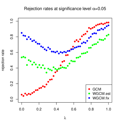
Figure 1: The plot shows the rejection rates at level $\alpha=0.05$ from $1000$ simulation runs of (7) with sample size $n=200$ for a range of $\lambda\in[0,1]$. The three methods GCM, WGCM.est and WGCM.fix are based on regressions using splines. For WGCM.est, we use $30\%$ of the samples to estimate the weight function $\operatorname{sign}(\mathbb{E}[\epsilon\xi|Z])$ and for WGCM.fix, we use $8$ fixed weight functions using our default choice described in Section 2.3.1.

To understand the phenomenon, let us consider the cases of $\lambda=1$ and $\lambda=0$ more closely. Using the notation from before, we have

$$\epsilon=X-\mathbb{E}[X|Z]=\eta_{X}$$

and

$$\xi=Y-\mathbb{E}[Y|Z]=\begin{cases}\eta_{Y}+0.3\eta_{X},&\lambda=1,\\ \eta_{Y}+0.15(2\eta_{X}Z+\eta_{X}^{2}-1),&\lambda=0.\end{cases}$$

If $\lambda=1$, we have $\mathbb{E}[\epsilon\xi]=0.3$, so we expect the GCM to have power in this case, which is also supported by our simulation. If $\lambda=0$, however, $\mathbb{E}[\epsilon\xi]=0$, since $\mathbb{E}[\eta_{X}\eta_{Y}]$, $\mathbb{E}[\eta_{X}^{2}Z]$ and $\mathbb{E}[\eta_{X}^{3}]$ are all equal to zero. Therefore, we do not expect the GCM to have power larger than the significance level $\alpha=0.05$ in this case, which is also visible in the plot. On the other hand, in the case of $\lambda=0$, we have that

$$\mathbb{E}[\epsilon\xi|Z]=0.3\mathbb{E}[\eta_{X}^{2}Z|Z]=0.3Z,$$

which is not almost surely equal to zero. Thus, we expect the two variants of the WGCM to have power. This is supported by the simulation.

1.2 Conventions and Notation

As most of the arguments are along the same lines as in Shah and Peters (2020), we also largely use the same notation.

We will use the following setting: Let $X$, $Y$ and $Z$ be random vectors taking values in $\mathbb{R}^{d_{X}}$, $\mathbb{R}^{d_{Y}}$ and $\mathbb{R}^{d_{Z}}$. For $i=1,\ldots,n$, let $(x_{i},y_{i},z_{i})$ be i.i.d. copies of $(X,Y,Z)$. Let $\mathbf{X}^{(n)}\in\mathbb{R}^{n\times d_{X}}$, $\mathbf{Y}^{(n)}\in\mathbb{R}^{n\times d_{Y}}$ and $\mathbf{Z}^{(n)}\in\mathbb{R}^{n\times d_{Z}}$ be the data matrices with rows $x_{i}$, $y_{i}$ and $z_{i}$, respectively.

Whereas at some places, we will also consider categorical $X$ and $Y$, for most of the time, we assume that the joint distribution of $(X,Y,Z)$ is absolutely continuous with respect to Lebesgue measure. Let $p(x,y,z)$ be the joint Lebesgue density of $(X,Y,Z)$.

We say that $X$ and $Y$ are conditionally independent given $Z$, written as

$$X{\perp\!\!\!\perp}Y|Z,$$

if one of the following two equivalent characterizations holds for Lebesgue almost all $(x,y,z)\in\mathbb{R}^{d_{X}}\times\mathbb{R}^{d_{Y}}\times\mathbb{R}^{d_{Z}}$ with $p(z)>0$:

1. $p(x,y|z)=p(x|z)p(y|z)$;

2. $p(x|y,z)=p(x|z)$,

see for example Section 3.1 in Dawid (1979).

Let $\mathcal{E}_{0}$ be the collection of all distributions for $(X,Y,Z)$ that are absolutely continuous with respect to Lebesgue measure. Let $\mathcal{P}_{0}\subseteq\mathcal{E}_{0}$ be the set of distributions in $\mathcal{E}_{0}$ such that $X$ and $Y$ are conditionally independent given $Z$.

We use $\mathbb{E}_{P}[\cdot]$ to denote the expectation of random variables under the probability distribution $P$ and we write $\mathbb{P}_{P}(\cdot)$ for the corresponding probability measure $\mathbb{E}_{P}\left[\mathbbm{1}{\{\cdot\}}\right]$. We denote indicator functions with $\mathbbm{1}\{\cdot\}$ or $\mathbbm{1}_{A}$.

We write $\Phi$ for the cumulative distribution function of a standard normal random variable, that is, for all $x\in\mathbb{R}$, we have $\Phi(x)=\mathbb{P}(X\leq x)$, where $X\sim\mathcal{N}(0,1)$.

Let $\mathcal{P}$ be a collection of probability distributions. For a sequence of random variables $\left(V_{P,n}\right)_{n\in\mathbb{N},P\in\mathcal{P}}$ with laws determined by $P\in\mathcal{P}$, we write $V_{P,n}=o_{\mathcal{P}}(1)$ if for all $\epsilon>0$

$$\lim_{n\to\infty}\sup_{P\in\mathcal{P}}\mathbb{P}_{P}\left(|V_{n}|>\epsilon\right)=0.$$

We write $V_{P,n}=O_{\mathcal{P}}(1)$ if

$$\limsup_{M\to\infty}\sup_{P\in\mathcal{P}}\sup_{n\in\mathbb{N}}\mathbb{P}_{P}\left(|V_{n}|>M\right)=0.$$

For another sequence $\left(W_{P,n}\right)_{n\in\mathbb{N},P\in\mathcal{P}}$ of strictly positive random variables, we write $V_{P,n}=o_{\mathcal{P}}(W_{P,n})$ and $V_{P,n}=O_{\mathcal{P}}(W_{P,n})$ if $V_{P,n}/W_{P,n}=o_{\mathcal{P}}(1)$ and $V_{P,n}/W_{P,n}=O_{\mathcal{P}}(1)$, respectively.

For a random variable $Z$ taking values in (a subset of) $\mathbb{R}^{d_{Z}}$, we typically say for all $z\in\mathbb{R}^{d_{Z}}$ instead of for all $z$ in the support of $Z$.

1.3 Outline

In Section 2, we describe the WGCM for univariate $X$ and $Y$. After a motivation as an extension of the GCM, we present two variants of the WGCM. The first variant WGCM.est is based on sample splitting to estimate a weight function, whereas the second variant WGCM.fix uses multiple fixed weight functions and aggregates the results. We provide Theorems justifying level and power of the methods. In Section 3, we compare our methods to the original GCM using simulation and also apply the methods to some real data sets in the context of variable selection. In the appendix, we show, how the WGCM can be extended to the case of multivariate $X$ and $Y$ and present the proofs of our various results.

2 The Univariate Weighted Generalised Covariance Measure

In this section, we introduce the weighted generalised covariance measure (WGCM), which is an extension of the generalised covariance measure (GCM) recently introduced by Shah and Peters (2020). We first treat the case of $d_{X}=d_{Y}=1$ and present different variants of the WGCM in this case. In Appendix A, we give extensions for multivariate $X$ and $Y$.

2.1 Prerequisites

We consider the same setup as in Section 3.1 of Shah and Peters (2020).

Let $d_{X}=d_{Y}=1$ and $d_{Z}\geq 1$. For any distribution $P\in\mathcal{E}_{0}$, let $\epsilon_{P}=X-\mathbb{E}_{P}[X|Z]$ and $\xi_{P}=Y-\mathbb{E}_{P}[Y|Z]$ and for $z\in\mathbb{R}^{d_{Z}}$, define the functions $f_{P}(z)=\mathbb{E}_{P}[X|Z=z]$ and $g_{P}(z)=\mathbb{E}_{P}[Y|Z=z]$. Then, we can write

$$X=f_{P}(Z)+\epsilon_{P},\quad Y=g_{P}(Z)+\xi_{P}.$$

For $i=1,\ldots,n$, let $\epsilon_{P,i}=x_{i}-f_{P}(z_{i})$ and $\xi_{P,i}=y_{i}-g_{P}(z_{i})$. Moreover, let $u_{P}(z)=\mathbb{E}_{P}[\epsilon_{P}^{2}|Z=z]$ and $v_{P}(z)=\mathbb{E}_{P}[\xi_{P}^{2}|Z=z]$.

Let $\hat{f}^{(n)}$ and $\hat{g}^{(n)}$ be estimates of $f_{P}$ and $g_{P}$, obtained by regression of $\mathbf{X}^{(n)}$, respectively $\mathbf{Y}^{(n)}$ on $\mathbf{Z}^{(n)}$.

In the following, the dependence on $n$ and $P$ is sometimes omitted. The GCM by Shah and Peters (2020) uses the products of the residuals

$$R_{i}=\left(x_{i}-\hat{f}(z_{i})\right)\left(y_{i}-\hat{g}(z_{i})\vphantom{x_{i}-\hat{f}(z_{i})}\right),\quad i=1,\ldots,n$$

as the basis of the test statistic

$$T^{(n)}=\frac{\frac{1}{\sqrt{n}}\sum_{i=1}^{n}R_{i}}{\left(\frac{1}{n}\sum_{i=1}^{n}R_{i}^{2}-\left(\frac{1}{n}\sum_{r=1}^{n}R_{r}\right)^{2}\right)^{1/2}}\eqqcolon\frac{\tau_{N}^{(n)}}{\tau_{D}^{(n)}},$$ (8)

which is a normalised sum of the $R_{i}$. Under the null hypothesis $X{\perp\!\!\!\perp}Y|Z$ and suitable conditions on the convergence of $\hat{f}$ and $\hat{g}$ to $f$ and $g$, the test statistic $T^{(n)}$ converges in distribution to a standard normal random variable, see Theorem 6 in Shah and Peters (2020).

The test statistic of the GCM is a normalised estimate of $\mathbb{E}_{P}[\epsilon_{P}\xi_{P}]$. Under the null hypothesis of $X{\perp\!\!\!\perp}Y|Z$, we have

$$\mathbb{E}_{P}[\epsilon_{P}\xi_{P}|Z]=\mathbb{E}_{P}[\mathbb{E}_{P}[\xi_{P}|Z,X]\epsilon_{P}]=0,$$

using $\mathbb{E}_{P}[\xi|X,Z]=\mathbb{E}_{P}[\xi|X]$ a.s. However, it is also possible to have $\mathbb{E}_{P}[\epsilon_{P}\xi_{P}]=0$ and $X{\not\!\perp\!\!\!\perp}Y|Z$. Therefore, the GCM only has power against alternatives with $\mathbb{E}_{P}[\epsilon_{P}\xi_{P}]\neq 0$, see Theorem 8 in Shah and Peters (2020).

By introducing an additional weight function in the test statistic, one can modify the set of alternatives against which the test has power. Let $w:\mathbb{R}^{d_{Z}}\to\mathbb{R}$ be a bounded measurable function. If we use the weighted product of the residuals

$$R_{i}=\left(x_{i}-\hat{f}(z_{i})\right)\left(y_{i}-\hat{g}(z_{i})\vphantom{x_{i}-\hat{f}(z_{i})}\right)w(z_{i}),\quad i=1,\ldots,n$$

as the basis of the test statistic defined in (8), $T^{(n)}$ is now a normalised estimate of $\mathbb{E}_{P}[\epsilon_{P}\xi_{P}w(Z)]$. Under the null hypothesis of $X{\perp\!\!\!\perp}Y|Z$, we still have

$$\mathbb{E}_{P}[\epsilon_{P}\xi_{P}w(Z)]=\mathbb{E}_{P}[\mathbb{E}_{P}[\xi_{P}|Z,X]\epsilon_{P}w(Z)]=0,$$

but now, the test has power against alternatives with $\mathbb{E}_{P}[\epsilon_{P}\xi_{P}w(Z)]\neq 0$. A weight function $w$ with $\mathbb{E}_{P}[\epsilon_{P}\xi_{P}w(Z)]\neq 0$ exists if and only if $\mathbb{E}_{P}[\epsilon_{P}\xi_{P}|Z]$ is not almost surely equal to $0$, see Equation (1). Typically, $\mathbb{E}_{P}[\epsilon_{P}\xi_{P}|Z]$ is unknown, so we do not know a suitable weight function. A possible strategy is to perform sample splitting and estimate a weight function on the first part of the sample (WGCM.est). This approach is treated next. Another approach is to calculate the test statistic for multiple weight functions and then to aggregate the results (WGCM.fix). This will be treated in Section 2.3.

2.2 WGCM with Estimated Weight Function (WGCM.est)

We have seen in Equation (1) that a desirable weight function for the WGCM is for example $w(z)=\operatorname{sign}\left(\mathbb{E}[\epsilon\xi|Z=z]\right)$. We do not know $\mathbb{E}[\epsilon\xi|Z]$ in practice, but we can estimate it. We propose the following procedure:

Method 1 (WGCM.est)

Using one random sample split, create two independent data sets $(\mathbf{X}^{(n)},\mathbf{Y}^{(n)},\mathbf{Z}^{(n)})$ and $\mathbf{A}=(\mathbf{X}_{A},\mathbf{Y}_{A},\mathbf{Z}_{A})$. We use the data set $\mathbf{A}$ to estimate a weight function and calculate the test statistic on the data set $(\mathbf{X}^{(n)},\mathbf{Y}^{(n)},\mathbf{Z}^{(n)})$ as in Section 2.1. For ease of notation, we still assume that $(\mathbf{X}^{(n)},\mathbf{Y}^{(n)},\mathbf{Z}^{(n)})$ consists of $n$ samples, whereas the size $a_{n}$ of the data set $\mathbf{A}=(\mathbf{X}_{A},\mathbf{Y}_{A},\mathbf{Z}_{A})$ is arbitrary (but depends on $n$). The ratio between the sizes of the data sets $(\mathbf{X}^{(n)},\mathbf{Y}^{(n)},\mathbf{Z}^{(n)})$ and $\mathbf{A}$ is difficult to choose in practice. We propose to estimate a weight function as follows:

1. (Nonlinearly) regress $\mathbf{X}_{A}$ on $\mathbf{Z}_{A}$ to get $\hat{f}_{A}$ and $\mathbf{Y}_{A}$ on $\mathbf{Z}_{A}$ to get $\hat{g}_{A}$. Let $\hat{\epsilon}_{A,i}=x_{A,i}-\hat{f}_{A}(z_{A,i})$ and $\hat{\xi}_{A,i}=y_{A,i}-\hat{g}_{A}(z_{A,i})$.

2. (Nonlinearly) regress $\left(\hat{\epsilon}_{A,i}\hat{\xi}_{A,i}\right)_{i=1}^{a_{n}}$ on $\mathbf{Z}_{A}$ to get $\hat{h}$ which is an estimate of $h(\cdot)=\mathbb{E}_{P}[\epsilon\xi|Z=\cdot]$.

3. Set $\hat{w}^{(n)}(\cdot)=\operatorname{sign}(\hat{h}(\cdot))$.

The following two theorems do not assume this particular choice of $\hat{w}^{(n)}$ based on the $\operatorname{sign}$, but only require it to be estimated on a data set $\mathbf{A}$ independent of $(\mathbf{X}^{(n)},\mathbf{Y}^{(n)},\mathbf{Z}^{(n)})$. Note that the estimated weight function $\hat{w}^{(n)}$ is not required to converge for $n\to\infty$. This is important, since under the null hypothesis, we have $h(Z)=\mathbb{E}_{P}[\epsilon\xi|Z]=0$ a.s. Thus, an estimate of $w$ of the form $\hat{w}^{(n)}(\cdot)=\operatorname{sign}(\hat{h}(\cdot))$ will typically not converge under the null hypothesis.

We consider the setting of Section 2.1 with the difference of replacing $R_{i}$ by

$$R_{i}^{(n)}=\left(x_{i}-\hat{f}^{(n)}(z_{i})\right)\left(y_{i}-\hat{g}^{(n)}(z_{i})\right)\hat{w}^{(n)}(z_{i}),\quad i=1,\ldots,n,$$ (9)

and redefine the test statistic (8) by

$$T^{(n)}=\frac{\frac{1}{\sqrt{n}}\sum_{i=1}^{n}R_{i}^{(n)}}{\left(\frac{1}{n}\sum_{i=1}^{n}{R_{i}^{(n)}}^{2}-\left(\frac{1}{n}\sum_{r=1}^{n}R_{r}^{(n)}\right)^{2}\right)^{1/2}}\eqqcolon\frac{\tau_{N}^{(n)}}{\tau_{D}^{(n)}}.$$ (10)

2.2.1 Distribution Under the Null Hypothesis

We will repeatedly use the quantities

$$A_{f} =\frac{1}{n}\sum_{i=1}^{n}(f_{P}(z_{i})-\hat{f}(z_{i}))^{2}, A_{g} =\frac{1}{n}\sum_{i=1}^{n}(g_{P}(z_{i})-\hat{g}(z_{i}))^{2},$$ (11)

$$B_{f} =\frac{1}{n}\sum_{i=1}^{n}(f_{P}(z_{i})-\hat{f}(z_{i}))^{2}v_{P}(z_{i}), B_{g} =\frac{1}{n}\sum_{i=1}^{n}(g_{P}(z_{i})-\hat{g}(z_{i}))^{2}u_{P}(z_{i}).$$ (12)

The following theorem gives conditions under which the test statistic $T^{(n)}$ is asymptotically standard normal. In the case of constant weight function $w(z)=1$ (and without sample splitting), it reduces to Theorem 6 in Shah and Peters (2020).

Theorem 1 (WGCM.est)

Let $A_{f}$, $A_{g}$, $B_{f}$ and $B_{g}$ be defined as in (11) and (12). Assume that the weight function $\hat{w}^{(n)}$ is estimated on a data set $\mathbf{A}$ independent of $(\mathbf{X}^{(n)},\mathbf{Y}^{(n)},\mathbf{Z}^{(n)})$ and let $T^{(n)}$ be defined as in (10). Assume that there exists $C>0$ such that for all $n\in\mathbb{N}$ we have $|\hat{w}^{(n)}(z)|\leq C$ for all $z\in\mathbb{R}^{d_{Z}}$. Define

$$\bar{\sigma}_{n}^{2}=\bar{\sigma}_{n,P}^{2}=\mathbb{E}_{P}\left[\hat{w}^{(n)}(Z)^{2}\epsilon_{P}^{2}\xi_{P}^{2}|\mathbf{A}\right].$$

1. Let $P\in\mathcal{P}_{0}$. Assume that $A_{f}A_{g}=o_{P}(n^{-1})$, $B_{f}=o_{P}(1)$ and $B_{g}=o_{P}(1)$. If there exists $\eta>0$ such that $\mathbb{E}_{P}\left[|\epsilon_{P}\xi_{P}|^{2+\eta}\right]<\infty$ and if $P$-almost surely there exists $c>0$ such that $\inf_{n\in\mathbb{N}}\bar{\sigma}_{n}^{2}\geq c$, then

   $$\sup_{t\in\mathbb{R}}|\mathbb{P}_{P}(T^{(n)}\leq t)-\Phi(t)|\to 0.$$

2. Let $\mathcal{P}\subset\mathcal{P}_{0}$. Assume that $A_{f}A_{g}=o_{\mathcal{P}}(n^{-1})$, $B_{f}=o_{\mathcal{P}}(1)$ and $B_{g}=o_{\mathcal{P}}(1)$. If there exists $\eta>0$ such that $\sup_{P\in\mathcal{P}}\mathbb{E}_{P}\left[|\epsilon_{P}\xi_{P}|^{2+\eta}\right]<\infty$ and if there exists $c>0$ such that for all $P\in\mathcal{P}$, we have $P$-almost surely $\inf_{n\in\mathbb{N}}\bar{\sigma}_{n}^{2}\geq c$, then

   $$\sup_{P\in\mathcal{P}}\sup_{t\in\mathbb{R}}|\mathbb{P}_{P}(T^{(n)}\leq t)-\Phi(t)|\to 0.$$

A proof can be found in Appendix C.

Remark 2

1. An estimate of the form $\hat{w}^{(n)}(z)=\operatorname{sign}(\hat{h}^{(n)}(z))$ satisfies

   $$\mathbb{E}_{P}\left[\hat{w}^{(n)}(Z)^{2}\epsilon_{P}^{2}\xi_{P}^{2}|\mathbf{A}\right]=\mathbb{E}_{P}\left[\epsilon_{P}^{2}\xi_{P}^{2}\right]\text{ a.s.},$$

   so $\bar{\sigma}_{n}^{2}\geq c$ is satisfied.

2. It would be desirable to do both the estimation of the weight function and calculating the test statistic on the full sample. However, the condition that the weight functions are estimated on an independent data set cannot be removed in general. If the weight function was allowed to depend on $(\mathbf{X}^{(n)},\mathbf{Y}^{(n)},\mathbf{Z}^{(n)})$, one could take functions $\hat{w}^{(n)}$ with $\hat{w}^{(n)}(z_{i})=\operatorname{sign}\left((x_{i}-\hat{f}(z_{i}))(y_{i}-\hat{g}(z_{i}))\right)$. This would always lead to a positive test statistic, which would contradict the asymptotic normality under the null hypothesis.

3. The conditions on the quantities $A_{f}$, $A_{g}$, $B_{f}$ and $B_{g}$ are reasonably weak. It is for example enough if $\hat{f}$ and $\hat{g}$ have mean squared prediction error (MSPE) of order $o(n^{-1/2})$, see Remark 7 in Shah and Peters (2020). An MSPE of order $o(n^{-1/2})$ can for example be obtained for real-valued $Z$ with bounded support if $f$ and $g$ are Lipschitz continuous, see for example Györfi et al. (2002), or for high-dimensional $Z$ with sparse and linear $f$ and $g$, see for example Bühlmann and van de Geer (2011). Moreover, the rates can also be satisfied using kernel ridge regression, see Section 4 of Shah and Peters (2020).

2.2.2 Power

In order to state a general power result, we need to make additional assumptions. We follow the path of Theorem 8 in Shah and Peters (2020) and assume that $\hat{f}$ and $\hat{g}$ have been estimated on another additional data set independent of $(\mathbf{X}^{(n)},\mathbf{Y}^{(n)},\mathbf{Z}^{(n)})$ and $\mathbf{A}$. This means that we have three independent data sets involved.

1. An auxiliary data set to estimate $\hat{f}$ and $\hat{g}$.

2. The data set $(\mathbf{X}^{(n)},\mathbf{Y}^{(n)},\mathbf{Z}^{(n)})$ to calculate the test statistic.

3. The data set $\mathbf{A}$ to estimate the weight function $\hat{w}^{(n)}$.

Whereas the sample splitting, that is, the independence of the $\mathbf{A}$ and $(\mathbf{X}^{(n)},\mathbf{Y}^{(n)},\mathbf{Z}^{(n)})$ is important in practice, the auxiliary data set to estimate $\hat{f}$ and $\hat{g}$ is mainly needed for technical reasons. In practice, it is usually recommended to use the original version of WGCM.est used in Section 2.2.1, see also Section 3.1.1. in Shah and Peters (2020) for a more detailed discussion.

Theorem 3 (WGCM.est)

Consider the setup of Theorem 1. Let $A_{f}$, $A_{g}$, $B_{f}$ and $B_{g}$ be defined as in (11) and (12) with the difference that $\hat{f}$ and $\hat{g}$ have been estimated on an auxiliary data set independent of $(\mathbf{X}^{(n)},\mathbf{Y}^{(n)},\mathbf{Z}^{(n)})$ and $\mathbf{A}$. Assume that there exists $C>0$ such that for all $n\in\mathbb{N}$ we have $|\hat{w}^{(n)}(z)|\leq C$ for all $z\in\mathbb{R}^{d_{Z}}$. For $P\in\mathcal{E}_{0}$, let

$$\bar{\rho}_{P,n}=\mathbb{E}_{P}\left[\epsilon_{P}\xi_{P}\hat{w}^{(n)}(Z)|\mathbf{A}\right]\quad\text{and}\quad\bar{\sigma}_{n}^{2}=\bar{\sigma}_{P,n}^{2}=\operatorname{var}_{P}\left(\epsilon_{P}\xi_{P}\hat{w}^{(n)}(Z)|\mathbf{A}\right).$$

Then, the following holds:

1. Let $P\in\mathcal{E}_{0}$. Assume that $A_{f}A_{g}=o_{P}(n^{-1})$, $B_{f}=o_{P}(1)$ and $B_{g}=o_{P}(1)$. Assume that there exists $\eta>0$ such that $\mathbb{E}_{P}\left[|\epsilon_{P}\xi_{P}|^{2+\eta}\right]<\infty$ and that $P$-almost surely there exists $c>0$ such that $\inf_{n\in\mathbb{N}}\bar{\sigma}_{n}^{2}\geq c$. Then, we have

   $$\sup_{t\in\mathbb{R}}\left|\mathbb{P}_{P}\left(T^{(n)}-\sqrt{n}\frac{\bar{\rho}_{P,n}}{\tau_{D}^{(n)}}\leq t\right)-\Phi(t)\right|\to 0,$$

   where $\tau_{D}^{(n)}$ is defined in (8).

2. Let $\mathcal{P}\subset\mathcal{E}_{0}$. Assume that $A_{f}A_{g}=o_{\mathcal{P}}(n^{-1})$, $B_{f}=o_{\mathcal{P}}(1)$ and $B_{g}=o_{\mathcal{P}}(1)$. If there exists $\eta>0$ such that $\sup_{P\in\mathcal{P}}\mathbb{E}_{P}\left[|\epsilon_{P}\xi_{P}|^{2+\eta}\right]<\infty$ and if there exists $c>0$ such that for all $P\in\mathcal{P}$, we have $P$-almost surely $\inf_{n\in\mathbb{N}}\bar{\sigma}_{n}^{2}\geq c$, then

   $$\sup_{P\in\mathcal{P}}\sup_{t\in\mathbb{R}}\left|\mathbb{P}_{P}\left(T^{(n)}-\sqrt{n}\frac{\bar{\rho}_{P,n}}{\tau_{D}^{(n)}}\leq t\right)-\Phi(t)\right|\to 0.$$

A proof can be found in Appendix C.

Remark 4

If instead of estimating the weight function, one uses a fixed weight function $w$, Theorem 3 implies that if $\rho_{P}=\mathbb{E}_{P}[\epsilon_{P}\xi_{P}w(Z)]\neq 0$, the test statistic $T^{(n)}$ is of order $\sqrt{n}\frac{\rho_{P}}{\sigma_{P}}$. That is, if $\rho_{P}\neq 0$, the WGCM with fixed weight function $w$ has asymptotic power $1$ against alternative $P$.

We recommend to obtain $\hat{w}^{(n)}$ by estimating $w(z)=\operatorname{sign}(\mathbb{E}_{P}[\epsilon\xi|Z=z])$, for example using Method 1. Recall the notation $\mathcal{P}_{est}$ from (3). Fix $P\in\mathcal{P}_{est}$, that is, $\mathbb{E}_{P}[\epsilon\xi|Z]$ is not almost surely equal to $0$ and assume that we can consistently estimate $w(z)=\operatorname{sign}(\mathbb{E}_{P}[\epsilon\xi|Z=z])$, wherever $\mathbb{E}_{P}[\epsilon\xi|Z=z]\neq 0$, that is

$$\mathbb{E}_{P}\left[(\hat{w}^{(n)}(Z)-w(Z))^{2}\mathbbm{1}\{\mathbb{E}_{P}[\epsilon\xi|\mathbf{Z}]\neq 0\}|\mathbf{A}\right]\to 0\text{ in probability}.$$

Defining

$$\rho_{P}=\mathbb{E}_{P}[\epsilon\xi w(Z)]=\mathbb{E}_{P}[|\mathbb{E}_{P}[\epsilon\xi|Z]|]>0,$$

it follows that $\bar{\rho}_{P,n}-\rho_{P}=o_{P}(1)$, because by the Cauchy-Schwarz inequality

$$|\bar{\rho}_{P,n}-\rho_{P}| =\left|\mathbb{E}_{P}\left[\epsilon\xi(\hat{w}^{(n)}(Z)-w(Z))|\mathbf{A}\right]\right|$$

$$\leq\mathbb{E}_{P}\left[\epsilon^{2}\xi^{2}\right]^{1/2}\mathbb{E}_{P}\left[(\hat{w}^{(n)}(Z)-w(Z))^{2}\mathbbm{1}\{\mathbb{E}_{P}[\epsilon\xi|\mathbf{Z}]\neq 0\}|\mathbf{A}\right]^{1/2}.$$

Hence, with high probability, $\bar{\rho}_{P,n}$ is bounded away from $0$ and we arrive at the following corollary.

Corollary 5 (WGCM.est)

Let $P\in\mathcal{P}_{est}$, that is $\mathbb{E}_{P}[\epsilon_{P}\xi_{P}|Z]$ is not almost surely equal to $0$. In the setting of Theorem 3, assertion 1., assume that

$$\mathbb{E}_{P}\left[(\hat{w}^{(n)}(Z)-w(Z))^{2}\mathbbm{1}\{\mathbb{E}_{P}[\epsilon\xi|\mathbf{Z}]\neq 0\}|\mathbf{A}\right]\to 0\text{ in probability.}$$

Then, for all $M>0$,

$$\mathbb{P}_{P}(T^{(n)}\geq M)\to 1,$$

that is, WGCM.est has asymptotic power $1$ against alternative $P$ for any significance level $\alpha\in(0,1)$.

Remark 6

Under the conditions of Corollary 5, WGCM.est has asymptotic power $1$ for alternatives $P\in\mathcal{P}_{est}$. This is a larger class compared to the GCM, which has power against alternatives in the class $\mathcal{P}_{GCM}$, that is $\mathbb{E}_{P}[\epsilon\xi]\neq 0$.

1. However, with Method 1 our additional requirement that $w(z)=\operatorname{sign}(\mathbb{E}_{P}[\epsilon\xi|Z])$ can be consistently estimated is not straightforward to verify, since there are two regressions involved. Intuitively, we will have that for the regression in step 1 of Method 1, $\hat{\epsilon}_{A}\hat{\xi}_{A}$ is close to $\epsilon\xi$. Even if the regression method in 2 is consistent, we still need that it is also not too much affected by the difference between $\hat{\epsilon}_{A}\hat{\xi}_{A}$ and $\epsilon\xi$. This will depend on the regression method applied in step 2.

2. One could use the following observation to obtain an alternative method to estimate $\hat{w}^{(n)}$. By definition,

   $$\mathbb{E}_{P}[\epsilon\xi|Z]=\mathbb{E}_{P}[(X-f(Z))(Y-g(Z)|Z]=\mathbb{E}_{P}[XY|Z]-f(Z)g(Z).$$

   Hence, additionally to the functions $\hat{f}$ and $\hat{g}$, one could try to also estimate the function $\mathbb{E}_{P}[XY|Z=z]$ using a regression of $XY$ on $Z$. The consistency condition in Corollary 5 could then be replaced by consistency conditions for estimating $\hat{f}$, $\hat{g}$ and $\mathbb{E}[XY|Z=z]$ which might be easier to justify than for the two-step approach of Method 1. However, the estimation of $\operatorname{sign}(\mathbb{E}_{P}[\epsilon\xi|Z])$ seems to be less reliable for finite samples using this method compared to using Method 1, which also leads to reduced power.

2.2.3 Binary Variables

If $X$ and $Y$ are binary, we can use the same methodology to obtain a test that has asymptotic power 1 against any alternative, provided that the conditions of Theorem 5 and Corollary 5 hold.

Assume that $X$ and $Y$ take values in $\{0,1\}$. By (6), we have that $\mathbb{E}_{P}[\epsilon\xi|Z]=0$ a.s. if and only if $X{\perp\!\!\!\perp}Y|Z$. We thus obtain the following result for binary $X$ and $Y$.

Corollary 7 (WGCM.est, binary case)

Let $X$ and $Y$ be binary and assume that the distribution $P$ of $(X,Y,Z)$ satisfies $X{\not\!\perp\!\!\!\perp}Y|Z$. In the setting of Theorem 3, assertion 1., assume that $\mathbb{E}_{P}\left[(\hat{w}^{(n)}(Z)-w(Z))^{2}\mathbbm{1}\{\mathbb{E}_{P}[\epsilon\xi|\mathbf{Z}]\neq 0\}|\mathbf{A}\right]\to 0$ in probability. Then, for all $M>0$,

$$\mathbb{P}_{P}(T^{(n)}\geq M)\to 1,$$

that is, WGCM.est has asymptotic power $1$ against alternative $P$ for any significance level $\alpha\in(0,1)$.

Using dummy coding, this methodology can be extended to arbitrary categorical $X$ and $Y$ variables, see Appendix A.3.

2.3 WGCM With Several Fixed Weight Functions (WGCM.fix)

We consider an alternative to the sample splitting approach. We calculate the test statistic for several fixed weight functions and aggregate the results. Consider the same setting as in Section 2.1. Let $\{w_{k}\}_{k=1}^{K}$ be bounded functions from $\mathbb{R}^{d_{Z}}\to\mathbb{R}$. For $k=1,\ldots,K$, let $\mathbf{R}_{k}\in\mathbb{R}^{n}$ be the vector of products of the residuals weighted by $w_{k}$, that is,

$$\mathbf{R}_{k}^{(n)}=\left(\begin{array}[]{c}(x_{1}-\hat{f}(z_{1}))(y_{1}-\hat{g}(z_{1}))w_{k}(z_{1})\\ \vdots\\ (x_{n}-\hat{f}(z_{n}))(y_{n}-\hat{g}(z_{n}))w_{k}(z_{n})\end{array}\right).$$

Let $T_{k}^{(n)}$ be the test statistic of the WGCM based on the vector $\mathbf{R}_{k}^{(n)}$, that is,

$$T_{k}^{(n)}=\frac{\sqrt{n}\bar{\mathbf{R}}_{k}}{\left(\frac{1}{n}\|\mathbf{R}_{k}\|_{2}^{2}-\bar{\mathbf{R}}_{k}^{2}\right)^{1/2}}\eqqcolon\frac{\tau_{N,k}^{(n)}}{\tau_{D,k}^{(n)}},$$ (13)

where $\bar{\mathbf{R}}_{k}$ is the sample average of the coordinates of ${\mathbf{R}_{k}}$. Finally, let

$$\mathbf{T}^{(n)}=\left(T_{1}^{(n)},\ldots,T_{K}^{(n)}\right)^{T}.$$

For a fixed number $K$ of weight functions, the simplest approach would be to perform an individual test for each weight function $w_{k}$ and use Bonferroni correction to aggregate the $K$ $p$-values. With the aggregated test statistic

$$S_{n}=\max_{k=1,\ldots K}|T_{k}^{(n)}|,$$

the Bonferroni corrected $p$-value is therefore

$$p_{\textup{Bon}}^{(n)}=K\cdot 2\left(1-\Phi(S_{n})\right).$$

In this case, it is straightforward to obtain a variant of Theorem 1 (stating that $p_{Bon}^{(n)}$ is a conservative $p$-value) and a variant of Theorem 3 (stating that the method has asymptotic power 1 if there exists $k\in\{1,\ldots,K\}$ with $\mathbb{E}_{P}[\epsilon\xi w_{k}(Z)]\neq 0$).

However, we can also use more sophisticated methods to calculate a $p$-value for $S_{n}=\max_{k=1,\ldots K}|T_{k}^{(n)}|$. With $K$ fixed, it is possible to show that under the null hypothesis of $P\in\mathcal{P}_{0}$ (i.e. $X{\perp\!\!\!\perp}Y|Y$), the vector $\mathbf{T}^{(n)}$ converges to a multivariate Gaussian distribution. In fact, we go one step further and propose the same procedure as in Section 3.2 of Shah and Peters (2020), where the multivariate case of the (unweighted) GCM is treated. For technical reason, it is assumed that $K\geq 3$. We do not assume that $K$ is fixed, but it is allowed to grow with $n$. Define

$$\hat{\Sigma}_{kl}=\frac{\frac{1}{n}\mathbf{R}_{k}^{T}\mathbf{R}_{l}-\bar{\mathbf{R}}_{k}\bar{\mathbf{R}}_{l}}{\left(\frac{1}{n}\|\mathbf{R}_{k}\|_{2}^{2}-\bar{\mathbf{R}}_{k}^{2}\right)^{1/2}\left(\frac{1}{n}\|\mathbf{R}_{l}\|_{2}^{2}-\bar{\mathbf{R}}_{l}^{2}\right)^{1/2}}.$$

Let $\hat{\mathbf{T}}^{(n)}\in\mathbb{R}^{K}$ have a multivariate normal distribution with covariance matrix $\hat{\Sigma}$ and mean $0$. Let

$$\hat{S}_{n}=\max_{k=1,\ldots,K}|\hat{T}^{(n)}_{k}|$$

and let $\hat{G}_{n}$ be the quantile function of $\hat{S}_{n}$ given $\hat{\Sigma}$. Note that $\hat{G}_{n}$ is random and depends on the data. $\hat{G}_{n}$ can be approximated by simulation. Recent results by Nadarajah et al. (2019) also allow to calculate $\hat{G}_{n}$ analytically. For a significance level $\alpha\in(0,1)$ we propose the following test.

Method 2 (WGCM.fix)

Reject the null hypothesis $X{\perp\!\!\!\perp}Y|Z$ if $S_{n}>\hat{G}_{n}(1-\alpha)$. The corresponding $p$-value is given by

$$p^{(n)}_{\textup{WGCM.fix}}=1-\hat{G}_{n}^{-1}(S_{n})=\mathbb{P}_{P}(\hat{S}_{n}>s|\hat{\Sigma})\big{|}_{s=S_{n}}.$$

We need the following conditions on the errors $\epsilon_{P}$ and $\xi_{P}$. Let $B\geq 1$.

• $\max_{r=1,2}\mathbb{E}_{P}\left[|\epsilon_{P}\xi_{P}|^{2+r}/B^{r}\right]+\mathbb{E}_{P}\left[\exp(|\epsilon_{P}\xi_{P}|/B)\right]\leq 4$;

• $\max_{r=1,2}\mathbb{E}_{P}\left[|\epsilon_{P}\xi_{P}|^{2+r}/B^{r/2}\right]+\mathbb{E}_{P}\left[|\epsilon_{P}\xi_{P}|^{4}/B^{2}\right]\leq 4$;

• $B^{2}\left(\log(Kn)\right)^{7}/n\leq Cn^{-c}$ for some constants $C,c>0$ that do not depend on $P\in\mathcal{P}$.

We obtain the following theorem. It is the adaptation of Theorem 9 in Shah and Peters (2020) to our setting.

Theorem 8 (WGCM.fix)

Let $\mathcal{P}\subset\mathcal{P}_{0}$ and let $A_{f}$, $A_{g}$, $B_{f}$ and $B_{g}$ be defined as in (11) and (12). Assume that there exist $C,c\geq 0$ such that for all $n\in\mathbb{N}$ and $P\in\mathcal{P}$ there exists $B\geq 1$ such that either (A1a) and (A2) or (A1b) and (A2) hold. Furthermore, assume that there exist $C_{1},c_{1}>0$ (independent of $n$) such that for all $k=1,\ldots,K$ and $P\in\mathcal{P}$ we have $|w_{k}|\leq C_{1}$ and $\mathbb{E}_{P}[\epsilon_{P}^{2}\xi_{P}^{2}w_{k}(Z)^{2}]\geq c_{1}$. Assume that

$$A_{f}A_{g}=o_{\mathcal{P}}\left(n^{-1}\log(K)^{-2}\right),$$ (14)

$$B_{f}=o_{\mathcal{P}}\left(\log(K)^{-4}\right),\quad B_{g}=o_{\mathcal{P}}\left(\log(K)^{-4}\right).$$ (15)

Assume that there exist sequences $\left(\tau_{f,n}\right)_{n\in\mathbb{N}}$ and $\left(\tau_{g,n}\right)_{n\in\mathbb{N}}$ of real numbers such that

$$\max_{i=1,\ldots,n}|\epsilon_{P,i}|=O_{\mathcal{P}}(\tau_{g,n}),\quad A_{g}=o_{\mathcal{P}}\left(\tau_{g,n}^{-2}\log(K)^{-2}\right),$$ (16)

$$\max_{i=1,\ldots,n}|\xi_{P,i}|=O_{\mathcal{P}}(\tau_{f,n}),\quad A_{f}=o_{\mathcal{P}}\left(\tau_{f,n}^{-2}\log(K)^{-2}\right).$$ (17)

Then,

$$\sup_{P\in\mathcal{P}}\sup_{\alpha\in(0,1)}|\mathbb{P}_{P}(S_{n}\leq\hat{G}_{n}(\alpha))-\alpha|\to 0.$$

The proof can be found in Appendix D.

Remark 9

1. If the errors $\epsilon_{P}$ and $\xi_{P}$ are sub-Gaussian with parameters bounded by some $M>0$ independent of $P\in\mathcal{P}$, then by Lemma 39 in Appendix G, their product $\epsilon_{P}\xi_{P}$ has a sub-exponential distribution, with parameters bounded independent of $P\in\mathcal{P}$, see also Remark 10 in Shah and Peters (2020). A summary of results on sub-Gaussian and sub-exponential distributions can be found in Appendix G. If $\epsilon_{P}\xi_{P}$ is sub-exponential with bounded parameters, then condition (A1a) is satisfied: By Definition 38, 2., there exists $K_{2}>0$ such that for all $P\in\mathcal{P}$,

   $$\mathbb{E}_{P}\left[\exp(|\epsilon\xi|/K_{2})\right]\leq 2.$$

   For $B_{0}\geq 1$, we get that

   $$\mathbb{E}_{P}[|\epsilon\xi|^{2+r}/B_{0}^{r}]\leq 2(2+r)!K_{2}^{2+r}/B_{0}^{r}.$$

   Thus, we can choose $B_{0}\geq 1$ such that for $r=1,2$ we have $\mathbb{E}_{P}[|\epsilon\xi|^{2+r}/B_{0}^{r}]\leq 2$ and set $B=\max(K_{2},B_{0})$.

   If $\epsilon_{P}$ and $\xi_{P}$ are sub-Gaussian with bounded parameters, by Corollary 37, we also have

   $$\max_{i=1,\ldots,n}|\epsilon_{i}|=O_{P}\left(\sqrt{\log(n)}\right)\text{ and }\max_{i=1,\ldots,n}|\xi_{i}|=O_{P}\left(\sqrt{\log(n)}\right).$$

   If we for example have that both $A_{f},A_{g}=o_{\mathcal{P}}(n^{-1/2}\log(K)^{-2})$, then (14), (16) and (17) are satisfied. Alternatively, we can also work under the conditions of Theorem 11. Then, the corresponding Remark 12 holds.

2. Compared to Theorem 9 in Shah and Peters (2020), we are still in a simplified setting, because due to the boundedness of the $w_{k}$, we only need bounds on $\epsilon_{P}\xi_{P}$ instead of $\epsilon_{P,j}\xi_{P,l}$ for all combinations of $j=1,\ldots,d_{X}$ and $l=1,\ldots,d_{Y}$. This will change when we consider the multivariate case, see Theorem 11.

The approach WGCM.fix always yields a lower $p$-value than using Bonferroni correction. To see this, let $X=(X_{1},\ldots,X_{k})^{T}\sim N(0,\Sigma)$, for a covariance matrix $\Sigma$ with $\Sigma_{kk}=1$ for all $k=1,\ldots,K$. Then, we have for $s\geq 0$

$$\mathbb{P}_{P}\left(\max_{k=1,\ldots,K}|X_{k}|>s\right)=\mathbb{P}_{P}\left(\bigcup_{k=1}^{K}\{|X_{k}|>s\}\right)\leq\sum_{k=1}^{K}\mathbb{P}_{P}(|X_{k}|>s)=K\cdot 2\left(1-\Phi(s)\right).$$

By replacing $\Sigma$ with $\hat{\Sigma}$, and $s$ by $S_{n}$, it follows that $p^{(n)}_{\textup{WGCM.fix}}\leq p^{(n)}_{\textup{Bon}}$. As an immediate consequence of Theorem 3 and Remark 4, we get the following result on the power of WGCM.fix for a fixed number $K$ of weight functions. Recall the set $\mathcal{P}_{\mathbf{W}}$ from (5).

Corollary 10 (WGCM.fix)

Let $P\in\mathcal{E}_{0}$. Let $A_{f}$, $A_{g}$, $B_{f}$ and $B_{g}$ be defined as in (11) and (12) with the difference that $\hat{f}$ and $\hat{g}$ have been estimated on an auxiliary data set independent of $(\mathbf{X}^{(n)},\mathbf{Y}^{(n)},\mathbf{Z}^{(n)})$. Let $K\geq 1$ be fixed. Assume that there exists $C>0$ such that for all $z\in\mathbb{R}^{d_{Z}}$ and all $k=1,\ldots,K$, we have $|w_{k}(z)|\leq C$. Assume that $A_{f}A_{g}=o_{P}(n^{-1})$, $B_{f}=o_{P}(1)$ and $B_{g}=o_{P}(1)$ as well as $\mathbb{E}_{P}[\epsilon_{P}^{2}\xi_{P}^{2}w_{k}(Z)^{2}]>0$ for all $k=1,\ldots,K$ and $\mathbb{E}_{P}\left[\epsilon_{P}^{2}\xi_{P}^{2}\right]<\infty$. If $P\in\mathcal{P}_{\mathbf{W}}$ for $\mathbf{W}=\{w_{1},\ldots,w_{K}\}$, that is if there exists $k\in\{1,\ldots,K\}$ such that $\mathbb{E}_{P}[\epsilon_{P}\xi_{P}w_{k}(Z)]\neq 0$, then for all $M>0$,

$$\mathbb{P}_{P}(S_{n}\geq M)\to 1,$$

that is, WGCM.fix with fixed number $K$ of weight functions has asymptotic power $1$ against alternative $P$ for any significance level $\alpha\in(0,1)$.

2.3.1 Choice of Weight Functions

We give a few heuristics on how to choose the weight functions in practice.

For a fixed alternative $P\in\mathcal{E}_{0}$, a promising weight function $w:\mathbb{R}^{d_{Z}}\to\mathbb{R}$ satisfies $\mathbb{E}_{P}[\epsilon\xi w(Z)]\neq 0$. We know, that such a $w$ exists if and only if $\mathbb{E}_{P}[\epsilon\xi|Z]$ is not almost surely equal to $0$.

Let us first assume that $d_{Z}=1$. For $a\in\mathbb{R}$, define the functions

$$w_{a}(z)=\operatorname{sign}(z-a)=\begin{cases}-1,&z<a\\ 1,&z\geq a.\end{cases}$$

Then, we have that $\mathbb{E}_{P}[\epsilon\xi|Z]=0$ a.s. if and only if $\mathbb{E}_{P}[\epsilon\xi w_{a}(Z)]=0$ for all $a$ in the support of $Z$. To see this, define $h(z)=\mathbb{E}_{P}[\epsilon\xi|Z=z]$. Then,

$$\mathbb{E}_{P}[\epsilon\xi w_{a}(Z)]=\mathbb{E}_{P}[h(Z)w_{a}(Z)]\\ =\int_{a}^{\infty}h(z)p_{Z}(z)\text{d}z-\int_{-\infty}^{a}h(z)p_{Z}(z)\text{d}z.$$

If $\mathbb{E}_{P}[\epsilon\xi w_{a}(Z)]=0$ for all $a$ in the support of $Z$, then taking the derivative with respect to $a$ yields $h(z)=0$ for all $z$ in the support of $Z$.

Therefore, it intuitively seems a good idea (in addition to the constant weight function $w(z)=1$) to use the functions $w_{a_{1}},\ldots,w_{a_{K-1}}$ for some $a_{1},\ldots,a_{K-1}\in\mathbb{R}$. In practice, one can for example take $a_{1},\ldots,a_{K-1}$ at the empirical $\frac{1}{K},\ldots,\frac{K-1}{K}$-quantiles of $Z$. However, the choice of $K$ is a difficult problem. Theorem 8 allows for $K$ to be large compared to $n$. However, if $K$ is too large, one is in danger of performing too many tests and loosing power again. This tradeoff makes the choice of $K$ difficult. In practice, we have experienced that a small number of weight functions is usually sufficient. For the experiments in Section 3, we will use $K=8$ weight functions.

For $d_{Z}>1$, one can for example take functions

$$w_{d,k}(\mathbf{z})=\operatorname{sign}(z_{d}-a_{d,k}),\,d=1,\ldots,d_{Z},\,k=1,\ldots,k_{0},$$

where $a_{d,k}$ is the empirical $\frac{k}{k_{0}+1}$-quantile of $Z_{j}$. This means that including the constant weight function $w(z)=1$, we have $K=k_{0}\cdot d_{Z}+1$ weight functions in total. For the experiments in Section 3, we will use $k_{0}=7$ weight functions per dimension of $Z$.

3 Experiments

We implement all our methods in R. Our implementations are based on the functions from the package GeneralisedCovarianceMeasure, see Peters and Shah (2019). Our code is available as the R-package weightedGCM on CRAN.

3.1 Detailed Comparison

We have seen that for the introductory example in Section 1.1.2, the power of the GCM heavily depends on the function introducing the dependence, whereas WGCM.est and WGCM.fix are more stable in this respect. To investigate the observed effect more systematically, we consider a family of functions $h_{b_{1},b_{2}}(t)$ indexed by two parameters $b_{1},b_{2}\in[0,1]$, where $b_{1}$ is a parameter for symmetry and $b_{2}$ is a parameter for wiggliness. Define

$$h_{1}(t,b_{1},b_{2}) =(b_{1}\cos(3b_{2}t)+(1-b_{1})\sin(3b_{2}t))\exp(-t^{2}/2),$$

$$h_{2}(t,b_{1}) =0.3(b_{1}|t|+(1-b_{1})t)$$

and let

$$h_{b_{1},b_{2}}(t)=(1-b_{2})h_{2}(t,b_{1})-b_{2}h_{1}(t,b_{1},b_{2}).$$

Plots of the functions $h_{b_{1},b_{2}}$ for various values of $b_{1}$ and $b_{2}$ can be found in Figure 2.

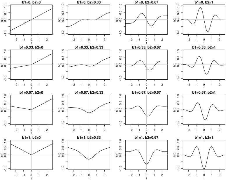
Figure 2: Plots of $h_{b_{1},b_{2}}$ for $b_{1},b_{2}\in\left\{0,\frac{1}{3},\frac{2}{3},1\right\}$.

3.1.1 Null Hypothesis

We first look at the level of the tests under the null hypothesis in the following three settings, which are similar to Section 5.2 in Shah and Peters (2020):

• $Z\sim\mathcal{N}(0,1),\,X=h_{b_{1},b_{2}}(Z)+0.3\mathcal{N}(0,1),\,Y=h_{b_{1},b_{2}}(Z)+0.3\mathcal{N}(0,1)$;

• $Z_{1},\ldots,Z_{10}\sim\mathcal{N}(0,1),\,X=h_{b_{1},b_{2}}(Z_{1})-h_{b_{1},b_{2}}(Z_{2})+0.3\mathcal{N}(0,1),\,Y=h_{b_{1},b_{2}}(Z_{1})+h_{b_{1},b_{2}}(Z_{2})+0.3\mathcal{N}(0,1)$;

• $Z_{1},\ldots,Z_{10}\sim\mathcal{N}(0,1),\,X=\operatorname{sign}\left(h_{b_{1},b_{2}}(Z_{1})+h_{b_{1},b_{2}}(Z_{2})\right)+0.3\mathcal{N}(0,1),\,Y=\operatorname{sign}\left(h_{b_{1},b_{2}}(Z_{1})-h_{b_{1},b_{2}}(Z_{2})\right)+0.3\mathcal{N}(0,1)$;

For every combination of $b_{1},b_{2}\in\left\{0,\frac{1}{3},\frac{2}{3},1\right\}$, we simulate $500$ data sets with $n$ samples for each setting and perform the following tests:

• The (unweighted) GCM by Shah and Peters (2020).

• The WGCM with one single estimated weight function, where $30\%$ of the samples are used to estimate the weight function.

• The WGCM with fixed weight functions

  $$w_{j,l}(z)=\operatorname{sign}(z_{j}-a_{j,l}),\,j=1,\ldots,d_{Z},\,l=1,\ldots,k_{0},$$

  where $a_{j,l}$ is the empirical $\frac{l}{k_{0}+1}$-quantile of $Z_{j}$. Additionally, we take the constant weight function $w_{0}(z)=1$. We will use $k_{0}=7$. This means we have a total of $8$ weight functions in the setting (1D) and $71$ weight functions in the settings (10D.Add) and (10D.NonAdd).

We perform all three tests both with regression splines using gam from the R package mgcv (see Wood, 2017) and with boosted regression trees using the package xgboost (see Chen and Guestrin, 2016 and Chen et al., 2021). For WGCM.est, we always use the same regression method both for step 1 and step 2 of Method 1 and for the calculation of the test statistic. Plots of the rejection rates at level $\alpha=0.05$ can be found in Figure 3. For each combination of setting and method, we plot the rejection rate for all 16 combinations of $b_{1}$ and $b_{2}$. The lower horizontal gray line denotes the individual one-sided test region at level $0.05$ for each dot based on a $Bin(500,0.95)$ distribution. The upper horizontal gray line denotes the joint one-sided test region at level $0.05$ for each group of $16$ dots based on $16$ i.i.d. $Bin(500,0.95)$ variables.

We see that with a sample size of $n=400$ and in the settings (1d) and (10dAdd), all the methods seem to perform reasonably well in the sense that the rejection rates are not significantly larger than $0.05$. In the setting (10dNonAdd), the methods based on gam seem to reject too often. This was to be expected since gam assumes an additive structure. For lower sample size, some of the methods seem to reject too often also in the settings (1d) and (10dAdd). The guarantees for the level of the tests heavily rely on the quality of the approximation of $\mathbb{E}[X|Z]$ and $\mathbb{E}[Y|Z]$. Therefore, we suspect that the large rejection rates in some settings with $n=100$ and $n=200$ are due to the fact that some of the functions used in the simulation are too complex to be well approximated with the smaller sample sizes.

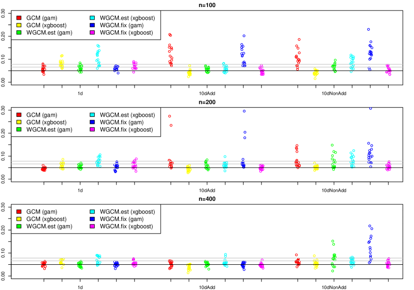
Figure 3: Rejection rates under the null hypothesis. For each combination of setting and method, every point corresponds to one of $16$ combinations of $b_{1},b_{2}\in\{0,\frac{1}{3},\frac{2}{3},1\}$. The rejection rates are calculated using 500 independent simulations. The two horizontal gray lines are at $0.066$ and $0.078$ and give individual and joint one-sided test regions at level $0.05$ for the null hypothesis ”the rejection rate of the test is less than or equal to $0.05$”: The value $0.066$ is the $0.95$-quantile of $B/500$, where $B\sim{Bin}(500,0.05)$ distribution, so the line denotes the test region of an individual dot. The value $0.078$ is the $0.95$-quantile of $\max(B_{1},\ldots,B_{16})/500$, where $B_{1},\ldots,B_{16}$ are i.i.d. ${Bin}(500,0.05)$, so the line denotes the joint test region for each group of $16$ dots.

3.1.2 Alternative Hypothesis

For the alternative, we consider the same settings (1D), (10D.Add), (10D.NonAdd), but modify them by adding $h_{c_{1},c_{2}}(X)$ to $Y$ for some $c_{1},c_{2}\in[0,1]$. We simulate 100 data sets for every combination of $b_{1},b_{2},c_{1},c_{2}\in\{0,\frac{1}{2},1\}$ and $n\in\{100,200,400\}$ and calculate the rejection rates of the methods GCM, WGCM.est and WGCM.fix both with gam and xgboost.

A significant difference to the simulations in Section 5.2 of Shah and Peters (2020) is that the function $h_{c_{1},c_{2}}(X)$ introducing the dependence is not just a linear function, but is also varied.

For each setting (1D), (10D.Add) and (10D.NonAdd), both regression methods gam and xgboost and sample sizes $n\in\{100,200,400\}$, we plot the rejection rates of the three methods GCM, WGCM.est and WGCM.fix against each other. Thus, each subplot consists of $9\cdot 9=81$ points, each corresponding to one combination of $b_{1}$, $b_{2}$, $c_{1}$ and $c_{2}$, see Figures 4, 5 and 6.

Let us first look at the first, second, fourth and fifth columns of the plots. These plot the rejection rates of GCM against the rejection rates of WGCM.est and WGCM.fix, respectively. We see that the behavior of the GCM and the two variants of the WGCM is asymmetric. The part on the bottom right of the corresponding plots is free, indicating that there are no situations where the GCM has a very high and the WGCM a very low rejection rate. In contrast, we see situations where the WGCM has a high, but the GCM a low rejection rate (points in the top left). The effect gets more pronounced for larger sample size. Nevertheless, there are also many points below the diagonal connecting $(0,0)$ and $(1,1)$. These indicate situations, where the GCM works better than the WGCM. To summarise, we see that indeed, the WGCM enlarges the space of alternatives against which the test has power. This comes at the cost of having less power in situations where the GCM already works well. In the setting (10D.NonAdd), the majority of the points lies below the diagonal in the plots comparing GCM to one of WGCM.fix and WGCM.est. As mentioned and observed in the simulations under the null hypothesis, we should not put too much trust in the results of (10D.NonAdd) with regression method gam. For the results using xgboost, it may also be possible that the picture would look more similar to the situations (1D) and (10D.Add) for larger sample size.

The third and sixth column of the plots compare the rejection rates of WGCM.est and WGCM.fix. We observe that WGCM.fix seems to perform better than WGCM.est, where the effect is more pronounced for (10D.Add) and (10D.NonAdd) than for (1D). However, by changing some parameters of the methods, for example the fraction of the samples used to estimate the weight function in WGCM.est and the number and type of weight functions for WGCM.fix, the picture could possibly look different.

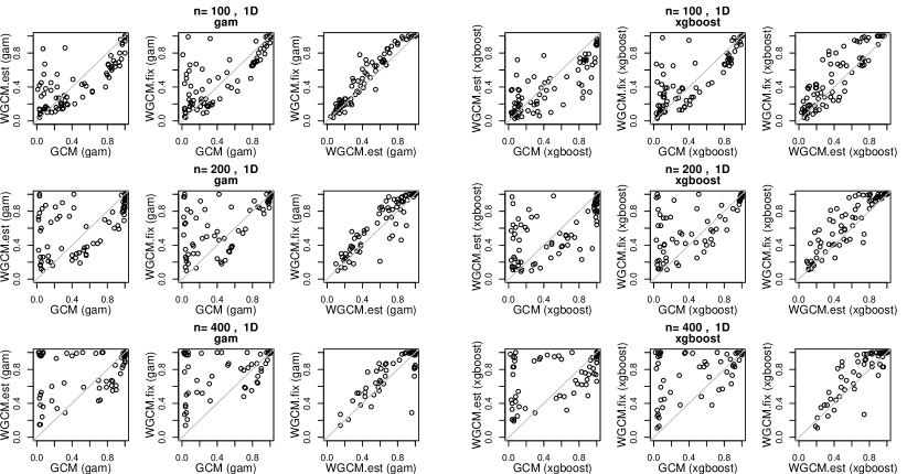
Figure 4: Rejection rates under the alternative hypothesis in situation (1D). The rejection rates of GCM, WGCM.est and WGCM.fix are plotted against each other for regression methods gam (left) and xgboost (right) and $n\in\{100,200,400\}$. Each subplot consists of $9\cdot 9=81$ points, each corresponding to one combination of $b_{1},b_{2},c_{1},c_{1}\in\{0,0.5,1\}$.

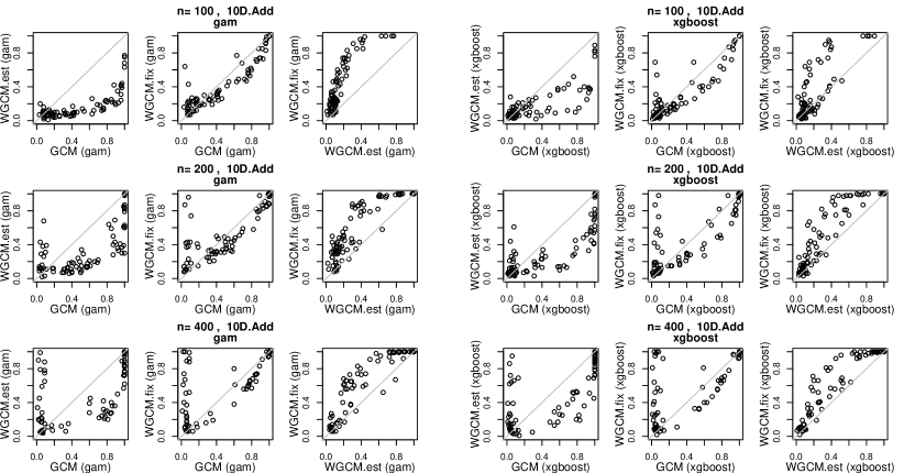
Figure 5: Rejection rates under the alternative hypothesis in situation (10D.Add). The rejection rates of GCM, WGCM.est and WGCM.fix are plotted against each other for regression methods gam (left) and xgboost (right) and $n\in\{100,200,400\}$. Each subplot consists of $9\cdot 9=81$ points, each corresponding to one combination of $b_{1},b_{2},c_{1},c_{1}\in\{0,0.5,1\}$.

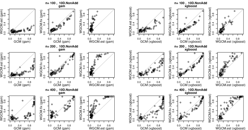
Figure 6: Rejection rates under the alternative hypothesis in situation (10D.NonAdd). The rejection rates of GCM, WGCM.est and WGCM.fix are plotted against each other for regression methods gam (left) and xgboost (right) and $n\in\{100,200,400\}$. Each subplot consists of $9\cdot 9=81$ points, each corresponding to one combination of $b_{1},b_{2},c_{1},c_{1}\in\{0,0.5,1\}$.

3.2 Variable Selection and Importance

In this section, we briefly sketch how conditional independence tests allow to perform variable selection tasks.

Suppose we have a response variable $Y$ and predictors $X_{j},j=1,\ldots,d$, where all random variables take values in $\mathbb{R}$. For all $j=1,\ldots,d$, we can test

$$H_{0}:X_{j}{\perp\!\!\!\perp}Y|\mathbf{X}_{-j}.$$

We expect the corresponding $p$-value to be small if $X_{j}$ yields additional information for predicting $Y$ that is not contained in $\mathbf{X}_{-j}$. This can be seen as a generalization of the individual $t$-tests in linear regression. We can then look, for which $j$ the variable $X_{j}$ is significant after a multiple testing correction. This approach is for example described in Watson and Wright (2019), where they compare it to a new method.

The following example is taken from Azadkia and Chatterjee (2019), where it appears as Example 7.4, with the difference that we only use a 50-dimensional $X$ and $n=500$ samples instead of a 1000-dimensional $X$ with $n=2000$ samples. We use GCM, WGCM.est and WGCM.fix with xgboost for the regressions.

Example 1

Let $X_{1},\ldots,X_{50}$ be i.i.d. $\mathcal{N}(0,1)$ and let $Y=X_{1}X_{2}+X_{1}-X_{3}+\epsilon$, where $\epsilon\sim\mathcal{N}(0,1)$ independent of $X_{1},\ldots,X_{50}$. We simulate $100$ data sets with a sample size of $n=500$. For each data set and all $j=1,\ldots,50$, we calculate a $p$-value for $H_{0}:X_{j}{\perp\!\!\!\perp}Y|\mathbf{X}_{-j}$ using the three tests. After a multiple testing correction using Holm’s procedure (Holm, 1979), we observe that GCM never finds the correct set of predictors at significance level $\alpha=0.05$, but most often, it just finds $X_{1}$ and $X_{3}$ as significant variables. WGCM.est finds the correct set of predictors in 86 out of 100 cases and WGCM.fix even finds the correct predictors in 99 of the 100 cases. We use the same type of weight functions with $k_{0}=7$ as in Section 3.1.1 for WGCM.fix and for WGCM.est, we use $30\%$ of the samples to estimate the weight functions.

Hence, this example illustrates that the two variants of the WGCM can find more dependencies than the GCM. In the following, we also look at some real data sets.

3.2.1 Boston Housing Data

As a first example, we analyse the Boston housing data, see Harrison and Rubinfeld (1978). Among the set of 13 predictors, we want to find the most relevant ones to predict the target variable medv, which is the median value of owner-occupied homes. Plots of the $p$-values after multiple testing correction using Holm’s method can be found in Figure 7. We performed all regressions using xgboost for GCM, WGCM.est and WGCM.fix

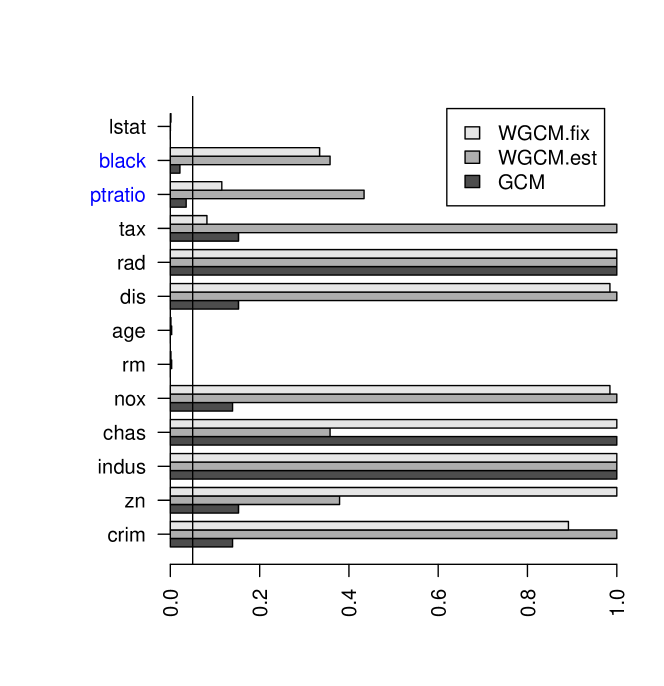
Figure 7: The $p$-values for the Boston housing data set for the prediction of the variable medv adjusted for multiple testing using Holm. For the variables denoted in blue, GCM shows a significant effect at level $\alpha=0.05$, but WGCM.fix and WGCM.est do not.

We see that in this case, the GCM finds $5$ significant variables at significance level $\alpha=0.05$, whereas WGCM.fix and WGCM.est only find $3$. Hence, this is an example where the original GCM performs moderately better (in terms of power) than the new variants.

3.2.2 Online News Popularity Data

We analyse the online news popularity data set, see Fernandes et al. (2015). The data can be obtained from the UCI Machine Learning Repository, see Dua and Graff (2017). Removing missing values, we have $39644$ observations of $58$ predictors and one target variable. Each observations corresponds to one article published by www.mashable.com. The target variable is the number of shares of the article, whereas the predictors are various features of the article, ranging from the number of words to sentiment scores. For the analysis, we take the log-transform of the target variable. Plots of the $p$-values for the three methods can be found in Figure 8. We performed the regressions using xgboost for GCM, WGCM.est and WGCM.est.

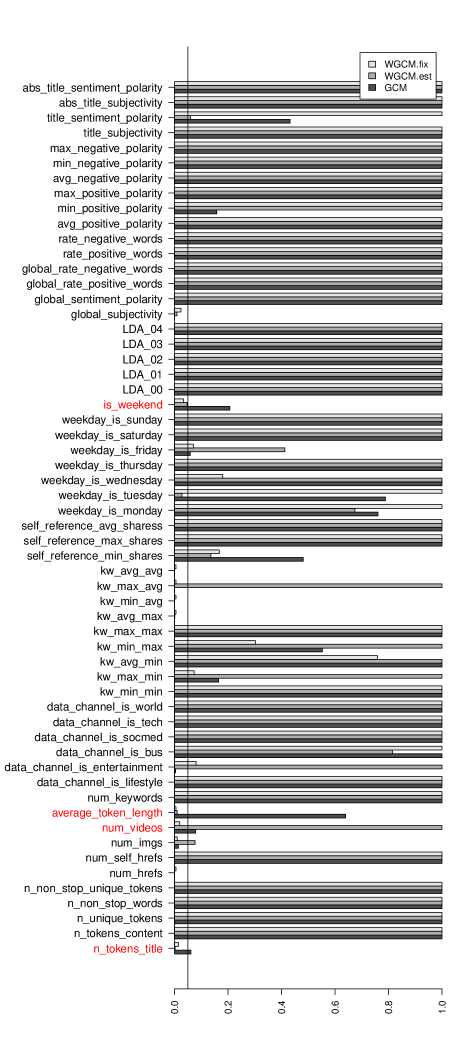
Figure 8: $p$-values for the online news popularity data set for the prediction of the variable shares adjusted for multiple testing using Holm. For the variables denoted in red, WGCM.fix shows a significant effect at level $\alpha=0.05$, but GCM does not.

We see that in this case, the GCM finds $8$ significant variables at significance level $\alpha=0.05$, whereas WGCM.est finds $9$ significant variables and WGCM.fix finds $11$ significant variables. Hence both versions of the WGCM perform slightly better (in terms of power) than the original GCM.

3.2.3 Wave Energy Converters Data

We look at the wave energy converters data set, available at the UCI Machine Learning Repository (Dua and Graff, 2017). The data set displays the (simulated) power output for different configurations of wave energy converters in different real wave scenarios, see Neshat et al. (2020). We restrict ourselves to the data of Tasmania. We have $32$ predictor variables, which consist of the $x$ and $y$-coordinates of $16$ wave energy converters forming a wave farm. The target is the total power output of the farm. We randomly sample $3000$ of the $72000$ configurations in the data set. By symmetry, it seems reasonable that either no or all predictor variables are significant. In fact, with Holm’s method to adjust for multiple testing, GCM does not find any significant predictor at significance level $\alpha=0.05$, whereas WGCM.fix considers all $32$ predictors significant and WGCM.est finds $11$ significant predictors. Plots of the $p$-values for the three methods can be found in Figure 9. In this case, the two WGCM methods are clearly superior to GCM (in terms of power).

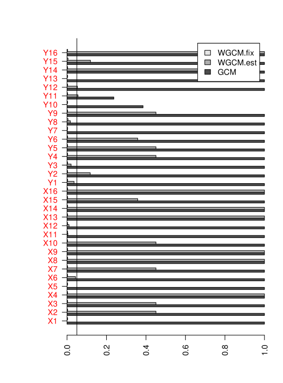
Figure 9: $p$-values of the predictor variables for the Tasmanian wave energy converters data set for the prediction of the total power output adjusted for multiple testing using Holm. At level $\alpha=0.05$, WGCM.fix finds a significant effect for all $32$ variables and WGCM.est for $11$ variables. GCM does not find any significant effect.

4 Conclusion

We have introduced the weighted generalised covariance measure (WGCM) as a new test for conditional independence and we provide an implementation in the R-package weightedGCM, which is available on CRAN. The WGCM is based on the generalised covariance measure (GCM) by Shah and Peters (2020). We gave two versions of the WGCM in the setting of univariate $X$ and $Y$. Their generalisations to the setting of multivariate $X$ and $Y$ can be found in Appendix A. To give guarantees for the correctness of the tests under appropriate conditions, we could benefit from the work by Shah and Peters (2020). We prove that WGCM.est and WGCM.fix have full asymptotic power against a broader class of alternatives than GCM. Finally, we compared our methods to the original GCM using simulation and on real data sets. We have seen for finite samples that our approach allows to enlarge the set of alternatives against which the test has power. This comes at the cost of having reduced power in settings where the GCM already performs well. An application in a variable selection task on real data sets confirmed that it depends on the data at hand which method is to be preferred. If the sample size is small and the form of the dependence is simple, the GCM will typically be the better choice. However, if the sample size is moderately large, choosing WGCM.fix or WGCM.est is typically beneficial.

4.1 Practical Issues

Choosing the optimal test among the GCM and the two versions of the WGCM remains a challenging task in practice, though it is always possible to perform several tests and use a multiple testing correction. It is worth mentioning that in principle, one could combine WGCM.est and WGCM.fix by including an estimated weight function together with the fixed weight functions of WGCM.fix. Such a case is implicitly covered by Theorem 14 in Appendix A.2. However, including an estimated weight function has the disadvantage that also the analysis of the fixed weight functions can only be done on half of the sample. For this reason, we think that performing the two tests WGCM.est and WGCM.fix individually and using Bonferroni correction is the better choice for combining the two tests.

Moreover, the randomness of the sample splitting for WGCM.est leads to the question how stable the test is with respect to this random split. We investigate this in Appendix B. Methods to aggregate $p$-values obtained from multiple sample splits are for example treated in Meinshausen et al. (2009) and in DiCiccio et al. (2020). The $p$-values obtained using such methods are more stable and provably controlling type I error. However, it is not clear how they affect the power of the test, even though the methods were found to improve power as well in other problems, see Meinshausen et al. (2009).

4.2 Outlook

There are many other open questions remaining. On the theoretical side, it would be desirable to give more concise results about the power properties of WGCM.est and WGCM.fix. For WGCM.est, Corollary 5 relies on the consistency of Method 1 to estimate $w(z)=\operatorname{sign}(\mathbb{E}_{P}[\epsilon\xi|Z=z])$, which is not straightforward to verify and depends on the regression method used. For WGCM.fix, it would be interesting to see, if there is a set of fixed weight functions with better properties than the ones described in Section 2.3.1.

On the practical side, there are many parameters that can be varied and whose effects could be inspected more closely. For WGCM.est, it would be desirable to have guidelines for the fraction of the data to be used to estimate the weight function. For WGCM.fix, the choice of the number of fixed weight functions is unknown for optimal power. However, our current default choice used in the empirical analysis seems to work reasonably well.

Also Method 1 to estimate the weight function could be investigated further. We do not claim our procedure to estimate $w(z)=\operatorname{sign}(\mathbb{E}_{P}[\epsilon\xi|Z=z])$ to be optimal. It is simply a straightforward way how the conditions of Theorem 1 can be satisfied. However, there might be more powerful procedures. It could be worth investigating if a smoothed version of the sign is beneficial. This would have the advantage of giving less weight to values of $z$ for which the estimate of $\mathbb{E}_{P}[\epsilon\xi|Z=z]$ is close to $0$ and which are thus more likely to obtain the wrong sign. However, the smoothed version of the sign still has to be scaled in such a way that the conditions for the correct null distribution are satisfied.

Acknowledgments

We are grateful to Rajen D. Shah for pointing out that WGCM.est has power against all alternatives for binary $X$ and $Y$. We thank Rajen D. Shah and Jonas Peters for answering our questions about their paper Shah and Peters (2020). We also thank three referees and an action editor for helpful comments. The research of Julia Hörrmann is supported by ETH Foundations of Data Science. Peter Bühlmann received funding from the European Research Council (ERC) under the European Union’s Horizon 2020 research and innovation programme (grant agreement No. 786461).

A The Multivariate WGCM

In this section, we show how the methods of Section 2.3 can also be applied in the case of multivariate $X$ and $Y$. This can be done both in the context of fixed and of estimated weight functions.

A.1 Multivariate WGCM With Fixed Weight Functions (mWGCM.fix)

The procedure is again very similar to Section 3.2 of Shah and Peters (2020). The idea in the case of multivariate $X$ and $Y$ stays the same, but we calculate the test statistic for every pair of $X_{j}$ and $Y_{l}$.

For any distribution $P\in\mathcal{E}_{0}$ and all $j=1,\ldots,d_{X}$ and $l=1,\ldots,d_{Y}$, define

$$f_{P,j}(z)=\mathbb{E}_{P}\left[X_{j}|Z=z\right]\quad\text{and}\quad g_{P,l}(z)=\mathbb{E}_{P}\left[Y_{l}|Z=z\right].$$

Then, we can write

$$X_{j}=f_{P,j}(Z)+\epsilon_{P,j}\quad\text{and}\quad Y_{l}=g_{P,l}(Z)+\xi_{P,l}.$$

Let $\epsilon_{P,ij}=x_{ij}-f_{P,j}(z_{i})$ and $\xi_{P,il}=y_{il}-g_{P,l}(z_{i})$.

Let $\hat{f}_{j}^{(n)}$ and $\hat{g}_{l}^{(n)}$ be estimates of $f_{P,j}$ and $g_{P,l}$, obtained by regression of $\mathbf{X}_{j}^{(n)}$ and $\mathbf{Y}_{l}^{(n)}$, on $\mathbf{Z}^{(n)}$. Note that $\mathbf{X}_{j}^{(n)}=(x_{1j},\ldots,x_{nj})^{T}$ is the $j$th column of the data matrix $\mathbf{X}^{(n)}$, or equivalently the column of samples from the random variable $X_{j}$.

For each $j,l$ let $K(j,l)\in\mathbb{N}$ and let $\left\{w_{jlk}:j=1,\ldots,d_{X},l=1,\ldots,d_{Y},k=1,\ldots,K(j,l)\right\}$ be functions from $\mathbb{R}^{d_{Z}}\to\mathbb{R}$. We allow $K(j,l)$ to grow with $n$. We will work under the assumption that the functions $w_{jlk}$ are uniformly bounded for all $j$, $l$ and $k$. Let

$$\mathbf{K}=\mathbf{K}(n)=\sum_{j=1}^{d_{X}}\sum_{l=1}^{d_{Y}}K(j,l).$$

Let $\mathbf{R}_{jlk}\in\mathbb{R}^{n}$ be the vector of products of the residuals corresponding to $X_{j}$ and $Y_{l}$ weighted by $w_{jlk}$, that is,

$$\mathbf{R}_{jlk}=\left(\begin{array}[]{c}(x_{1j}-\hat{f}_{j}(z_{1}))(y_{1l}-\hat{g}_{l}(z_{1}))w_{jlk}(z_{1})\\ \vdots\\ (x_{nj}-\hat{f}_{j}(z_{n}))(y_{nl}-\hat{g}_{l}(z_{n}))w_{jlk}(z_{n})\end{array}\right).$$

Let $T_{jlk}^{(n)}$ be the test statistic of the WGCM based on the vector $\mathbf{R}_{jlk}$, that is,

$$T_{jlk}^{(n)}=\frac{\sqrt{n}\bar{\mathbf{R}}_{jlk}}{\left(\frac{1}{n}\|\mathbf{R}_{jlk}\|_{2}^{2}-\bar{\mathbf{R}}_{jlk}^{2}\right)^{1/2}}\eqqcolon\frac{\tau_{N,{jlk}}^{(n)}}{\tau_{D,{jlk}}^{(n)}},$$ (18)

with $\bar{\mathbf{R}}_{jlk}$ being the sample average of the coordinates of ${\mathbf{R}_{jlk}}$. Finally, let $\mathbf{T}^{(n)}=\left(T_{jlk}^{(n)}\right)_{jlk}\in\mathbb{R}^{\mathbf{K}}$ be the vector of all test statistics. We consider the maximum absolute value of the vector $\mathbf{T}^{(n)}$ as a test statistic,

$$S_{n}=\max_{j=1,\ldots,d_{X},\,l=1,\ldots,d_{Y},\,k=1,\ldots,K(j,l)}|T_{jlk}^{(n)}|.$$

In summary, everything works similarly to the univariate case with the added complication of having expressions with three subscripts instead of one. Define $\hat{\Sigma}\in\mathbb{R}^{\mathbf{K}\times\mathbf{K}}$ by

$$\hat{\Sigma}_{jlk,j^{\prime}l^{\prime}k^{\prime}}=\frac{\frac{1}{n}\mathbf{R}_{jlk}^{T}\mathbf{R}_{j^{\prime}l^{\prime}k^{\prime}}-\bar{\mathbf{R}}_{jlk}\bar{\mathbf{R}}_{j^{\prime}l^{\prime}k^{\prime}}}{\left(\frac{1}{n}\|\mathbf{R}_{jlk}\|_{2}^{2}-\bar{\mathbf{R}}_{jlk}^{2}\right)^{1/2}\left(\frac{1}{n}\|\mathbf{R}_{j^{\prime}l^{\prime}k^{\prime}}\|_{2}^{2}-\bar{\mathbf{R}}_{j^{\prime}l^{\prime}k^{\prime}}^{2}\right)^{1/2}}.$$

Let $\hat{\mathbf{T}}^{(n)}=\left(\hat{T}_{jlk}^{(n)}\right)_{jlk}\in\mathbb{R}^{\mathbf{K}}$ have multivariate normal distribution with covariance $\hat{\Sigma}$ and mean $0$ and let

$$\hat{S}_{n}=\max_{j,l,k}|\hat{T}_{j,l,k}^{(n)}|.$$

Let $\hat{G}_{n}$ be the quantile function of $\hat{S}_{n}$ given $\hat{\Sigma}$. $\hat{G}_{n}$ is random, depends on the data and can be approximated by simulation. We need similar conditions to (A1a), (A1b) and (A2) for Theorem 8. Let

$$\sigma_{jl}^{2}=\sigma_{P,jl}^{2}=\mathbb{E}_{P}\left[\epsilon_{j}^{2}\xi_{l}^{2}\right].$$

Consider a sequence $(D_{n})_{n\in\mathbb{N}}$ with $D_{n}\geq 1$.

• $\max_{r=1,2}\mathbb{E}_{P}\left[\left|\frac{\epsilon_{j}\xi_{l}}{\sigma_{jl}}\right|^{2+r}/D_{n}^{r}\right]+\mathbb{E}_{P}\left[\exp\left(\left|\frac{\epsilon_{j}\xi_{l}}{\sigma_{jl}}\right|/D_{n}\right)\right]\leq 4$ for all $j=1,\ldots,d_{X}$, and $l=1,\ldots,d_{Y}$;

• $\max_{r=1,2}\mathbb{E}_{P}\left[\left|\frac{\epsilon_{j}\xi_{l}}{\sigma_{jl}}\right|^{2+r}/D_{n}^{r/2}\right]+\mathbb{E}_{P}\left[\max_{j,l}\left|\frac{\epsilon_{j}\xi_{l}}{\sigma_{jl}}\right|^{4}/D_{n}^{2}\right]\leq 4$ for all $j=1,\ldots,d_{X}$ and $l=1,\ldots,d_{Y}$;

• $D_{n}^{2}\left(\log(\mathbf{K}n)\right)^{7}/n\leq Cn^{-c}$ for some constants $C,c>0$ that do not depend on $P\in\mathcal{P}$.

We obtain the analogue of Theorem 8 (and also of Theorem 9 in Shah and Peters, 2020). For $j=1,\ldots,d_{X}$ and $l=1,\ldots,d_{Y}$, let

$$A_{f,j}=\frac{1}{n}\sum_{i=1}^{n}(f_{P,j}(z_{i})-\hat{f}_{j}(z_{i}))^{2},$$ (19)

$$A_{g,l}=\frac{1}{n}\sum_{i=1}^{n}(g_{P,l}(z_{i})-\hat{g}_{l}(z_{i}))^{2}.$$ (20)

Theorem 11 (mWGCM.fix)

Let $\mathcal{P}\subset\mathcal{P}_{0}$. Assume that there exist $C,c>0$ such that for all $n\in\mathbb{N}$ and $P\in\mathcal{P}$ there exists $D_{n}\geq 1$ such that either (C1a) and (C2) or (C1b) and (C2) hold. Furthermore, assume that there exist $C_{1},c_{1}>0$ (independent of $n$) such that for all $j=1,\ldots,d_{X}$, $l=1,\ldots,d_{Y}$ and $k=1,\ldots,K(j,l)$ and for all $P\in\mathcal{P}$, we have $|w_{jlk}|\leq C_{1}$ and $\mathbb{E}_{P}\left[\epsilon_{j}^{2}\xi_{l}^{2}w_{jlk}(Z)^{2}\right]\geq c_{1}\sigma_{jl}^{2}$. Assume that

$$\max_{j,l}\frac{1}{\sigma_{jl}^{2}}A_{f,j}A_{g,l}=o_{\mathcal{P}}\left(n^{-1}\log(\mathbf{K})^{-4}\right).$$ (21)

Assume that there exist sequences $\left(\tau_{f,n}\right)_{n\in\mathbb{N}}$ and $\left(\tau_{g,n}\right)_{n\in\mathbb{N}}$ as well as positive real numbers $s_{g,jl}$, $t_{g,jl}$, $s_{f,jl}$ and $t_{f,jl}$ possibly depending on $P\in\mathcal{P}$ such that for all $j=1,\ldots,d_{X}$, $l=1,\ldots,d_{Y}$

$$s_{f,jl}t_{f,jl}=\sigma_{jl},\quad s_{g,jl}t_{g,jl}=\sigma_{jl},$$

and such that

$$\max_{i,j,l}|\epsilon_{P,ij}|/t_{g,jl}=O_{\mathcal{P}}(\tau_{g,n}),\quad\max_{j,l}A_{g,l}/s_{g,jl}^{2}=o_{\mathcal{P}}\left(\tau_{g,n}^{-2}\log(\mathbf{K})^{-4}\right)$$ (22)

$$\max_{i,j,l}|\xi_{P,il}|/t_{f,jl}=O_{\mathcal{P}}(\tau_{f,n}),\quad\max_{j,l}A_{f,j}/s_{f,jl}^{2}=o_{\mathcal{P}}\left(\tau_{f,n}^{-2}\log(\mathbf{K})^{-4}\right).$$ (23)

Then,

$$\sup_{P\in\mathcal{P}}\sup_{\alpha\in(0,1)}|\mathbb{P}_{P}(S_{n}\leq\hat{G}_{n}(\alpha))-\alpha|\to 0.$$

Remark 12

1. The idea behind the sequences $s_{g,jl}$, $t_{g,jl}$, $s_{f,jl}$ and $t_{f,jl}$ is that they allow for a more general scaling than the simplified setting in the next item. Note that by $X{\perp\!\!\!\perp}Y|Z$, we have that $\sigma_{jl}^{2}=\mathbb{E}_{P}\left[u_{P,j}(Z)v_{P,l}(Z)\right]$, where $u_{P,j}(Z)=\mathbb{E}_{P}[\epsilon_{P,j}^{2}|Z]$ and $v_{P,l}(Z)=\mathbb{E}_{P}[\xi_{P,l}^{2}|Z]$. If for example $u_{P,j}(Z)$ and $v_{P,l}(Z)$ are a.s. constant equal to some $u_{j}$ and $v_{l}\in\mathbb{R}$, we can take $t_{g,jl}^{2}=s_{f,jl}^{2}=u_{j}$ and $t_{f,jl}^{2}=s_{g,jl}^{2}=v_{l}$. In this case, conditions (22) and (23) are just conditions on the errors $\epsilon_{j}$, $\xi_{l}$ scaled by their standard deviation and on $A_{f,j}$, $A_{g,l}$ scaled by the error variance.

2. Assume that there exists $c_{2}>0$ independent of $n$ such that for all $P\in\mathcal{P}$, all $j=1,\ldots,d_{X}$ and $l=1,\ldots,d_{Y}$ we have

   $$\sigma_{P,jl}=\mathbb{E}_{P}\left[\epsilon_{j}^{2}\xi_{l}^{2}\right]\geq c_{2}.$$ (24)

   Then, we can replace $\epsilon_{j}\xi_{l}/\sigma_{jl}$ by $\epsilon_{j}\xi_{l}$ in conditions (C1a), (C1b) and (C2). Furthermore, we can replace the sequences $s_{g,jl}$, $t_{g,jl}$, $s_{f,jl}$ and $t_{f,jl}$ by $1$ in conditions (22) and (23) and we can replace condition (21) by

   $$\max_{j,l}A_{f,j}A_{g,l}=o_{\mathcal{P}}\left(n^{-1}\log(\mathbf{K})^{-2}\right),$$

   see also the next item.

   If in addition to (24), we also have that the errors $\epsilon_{P,j}$ and $\xi_{P,l}$ have sub-Gaussian distributions with parameters uniformly bounded for all $j,l$ by some constant independent of $P\in\mathcal{P}$, then using the same arguments as in Remark 9, condition (C1a) can be satisfied with $D_{n}$ constant independent of $n$. Moreover, we have that $\max_{i,j}|\epsilon_{P,ij}|=O_{\mathcal{P}}\left(\sqrt{\log(nd_{X})}\right)$. If for example both

   $$\max_{j}A_{f,j},\max_{l}A_{g,l}=o_{\mathcal{P}}\left(\log(\mathbf{K})^{-4}\min(n^{-1/2},\log(\mathbf{K})^{-1})\right),$$

   then the modified versions of conditions (21), (22) and (23) are all satisfied.

3. If there exists $C_{3}>0$ such that for all $P\in\mathcal{P}$ and all $j,j^{\prime}=1,\ldots,d_{X}$ and $l,l^{\prime}=1,\ldots,d_{Y}$ we have

   $$\sigma_{jl}\sigma_{j^{\prime}l^{\prime}}\geq C_{3}\sigma_{jl^{\prime}}\sigma_{j^{\prime}l},$$

   then inspection of the proof shows that condition (21) can be replaced by

   $$\max_{j,l}\frac{1}{\sigma_{jl}^{2}}A_{f,j}A_{g,l}=o_{\mathcal{P}}\left(n^{-1}\log(\mathbf{K})^{-2}\right).$$

In analogy to Corollary 10, we obtain the following result about the power of mWGCM.fix if $d_{X}$, $d_{Y}$ and all $K(j,l)$ for $j=1,\ldots,d_{X}$ and $l=1,\ldots,d_{Y}$ are fixed. For this, let $u_{P,j}(Z)=\mathbb{E}_{P}[\epsilon_{P,j}^{2}|Z]$ and $v_{P,l}(Z)=\mathbb{E}_{P}[\epsilon_{P,l}^{2}|Z]$ and define

$$B_{f,jl}=\frac{1}{n}\sum_{i=1}^{n}(f_{P,j}(z_{i})-\hat{f}_{j}(z_{i}))^{2}v_{P,l}(z_{i}),$$ (25)

$$B_{g,jl}=\frac{1}{n}\sum_{i=1}^{n}(g_{P,l}(z_{i})-\hat{g}_{l}(z_{i}))^{2}u_{P,j}(z_{i}).$$ (26)

Corollary 13 (mWGCM.fix)

Let $P\in\mathcal{E}_{0}$. Let $A_{f,j}$, $A_{g,l}$, $B_{f,jl}$ and $B_{g,jl}$ be defined as in (19), (20), (25) and (26) with the difference that all $\hat{f}_{j}$ and $\hat{g}_{l}$ have been estimated on an auxiliary data set independent of $(\mathbf{X}^{(n)},\mathbf{Y}^{(n)},\mathbf{Z}^{(n)})$. Let $d_{X}$, $d_{Y}$ and all $K(j,l)$ for $j=1,\ldots,d_{X},\,l=1,\ldots,d_{Y}$ be fixed. Assume that there exists $C>0$ such that for all $z\in\mathbb{R}^{d_{Z}}$ and all $j,l,k$, we have $|w_{jlk}(z)|\leq C$. Assume that for all $j,l$ we have $A_{f,j}A_{g,l}=o_{P}(n^{-1})$, $B_{f,jl}=o_{P}(1)$ and $B_{g,jl}=o_{P}(1)$ as well as $\mathbb{E}_{P}[\epsilon_{P,j}^{2}\xi_{P,l}^{2}w_{jlk}(Z)^{2}]>0$ for all $k=1,\ldots,K(j,l)$ and $\mathbb{E}_{P}\left[\epsilon_{P,j}^{2}\xi_{P,l}^{2}\right]<\infty$. If there exists $j\in\{1,\ldots,d_{X}\},\,l\in\{1,\ldots,d_{Y}\}$ and $k\in\{1,\ldots,K(j,l)\}$ such that $\mathbb{E}_{P}[\epsilon_{P,j}\xi_{P,l}w_{k}(Z)]\neq 0$, then for all $M>0$,

$$\mathbb{P}_{P}(S_{n}\geq M)\to 1,$$

that is, mWGCM.fix with fixed $d_{X}$, $d_{Y}$ and fixed number of weight functions $K(j,l)$ for all $j$ and $l$ has asymptotic power $1$ against alternative $P$ for any significance level $\alpha\in(0,1)$.

A.1.1 Choice of weight functions

As the simplest extension of the considerations in Section 2.3.1, we propose the following. For a fixed $k_{0}\geq 1$ and every combination of $j=1,\ldots,d_{X}$ and $l=1,\ldots,d_{Y}$, use the same $K(j,l)=k_{0}\cdot d_{Z}+1$ weight functions

$$w(\mathbf{z})=1,\text{ and }w_{d,k}(\mathbf{z})=\operatorname{sign}(z_{d}-a_{d,k}),\,d=1,\ldots,d_{Z},\,k=1,\ldots,k_{0},$$

where $a_{d,k}$ is the empirical $\frac{k}{k_{0}+1}$-quantile of $Z_{d}$. This yields a total of $\mathbf{K}=d_{X}d_{Y}\cdot(k_{0}\cdot d_{Z}+1)$ weight functions, but the weight functions do not depend on $j$ and $l$.

A.2 Multivariate WGCM With Estimated Weight Functions

The same procedure can be applied with estimated weight functions. We consider the same setting as in Section A.1.

The difference is that the weight functions have been estimated on an auxiliary data set $\mathbf{A}$ independent of $(\mathbf{X}^{(n)},\mathbf{Y}^{(n)},\mathbf{Z}^{(n)})$, obtained for example by sample splitting as in Section 2.2. For each $j,l$, let $K(j,l)\in\mathbb{N}$, and for each $n\in\mathbb{N}$, let

$$\left\{\hat{w}_{jlk}^{(n)}:j=1,\ldots,d_{X},l=1,\ldots,d_{Y},k=1,\ldots,K(j,l)\right\}$$

be functions from $\mathbb{R}^{d_{Z}}\to\mathbb{R}$ that have been estimated on $\mathbf{A}$. In general, we would recommend to set $K(j,l)=1$ and use Method 1 to estimate $w_{j,l}(z)=\operatorname{sign}(\mathbb{E}_{P}[\epsilon_{j}\xi_{l}|Z=z]$. However, Theorem 14 even allows for $K(j,l)$ to grow with $n$. Let

$$\mathbf{K}=\mathbf{K}(n)=\sum_{j=1}^{d_{X}}\sum_{l=1}^{d_{Y}}K(j,l).$$

As in Section A.1, define based on the weight functions $\hat{w}_{jlk}^{(n)}$

• the vectors of weighted products of residuals $\mathbf{R}_{jlk}$;

• the test statistics $T_{jlk}^{(n)}$ of the individual WGCM;

• the aggregated test statistic $S_{n}$;

• the estimated covariance matrix $\hat{\Sigma}$;

• the multivariate normal vector $\hat{\mathbf{T}}^{(n)}$ and $\hat{S}_{n}$, the maximum absolute value of the components of $\hat{\mathbf{T}}^{(n)}$;

• the quantile function $\hat{G}_{n}$ of $\hat{S}_{n}$ given $\hat{\Sigma}$.

We have the following variant of Theorem 11. Remark 12 also applies to this theorem.

Theorem 14 (mWGCM.est)

Let $\mathcal{P}\subset\mathcal{P}_{0}$ and assume there exist $C,c>0$ such that for all $n\in\mathbb{N}$ and $P\in\mathcal{P}$ there exists $D_{n}\geq 1$ such that either (C1a) and (C2) or (C1b) and (C2) hold. Assume that the conditions (21), (22) and (23) are satisfied. Assume that there exist $C_{1},c_{1}>0$ (independent of $n$) such that for all $P\in\mathcal{P}$ we have $P$-almost surely for all $j,l,k$ and $n$

$$|\hat{w}_{jlk}^{(n)}(z)|\leq C_{1}\text{ for all }z\in\mathbb{R}^{d_{z}}$$

and

$$\mathbb{E}_{P}\left[\epsilon_{j}^{2}\xi_{l}^{2}\hat{w}_{jlk}^{(n)}(Z)^{2}|\mathbf{A}\right]\geq c_{1}\mathbb{E}_{P}\left[\epsilon_{j}^{2}\xi_{l}^{2}\right].$$

Then,

$$\sup_{P\in\mathcal{P}}\sup_{\alpha\in(0,1)}|\mathbb{P}_{P}(S_{n}\leq\hat{G}_{n}(\alpha))-\alpha|\to 0.$$

A proof can be found in Appendix E.

In the case of fixed $d_{X}$, $d_{Y}$ and if $K(j,l)=1$ for all $j=1,\ldots,d_{X}$ and $l=1,\ldots,d_{Y}$, we have a combination of Corollary 5 and Corollary 13. We assume, that we use Method 1 to estimate $w_{jl}(\cdot)=\operatorname{sign}(\mathbb{E}_{P}[\epsilon_{j}\xi_{l}|Z=\cdot])$. We denote the estimate of $w_{jl}$ by $\hat{w}^{(n)}_{jl}$. Note that we write $w_{jl}$ and not $w_{jlk}$, since $K(j,l)=1$ for all $j,l$.

Corollary 15 (mWGCM.est)

Let $P\in\mathcal{E}_{0}$. Let $A_{f,j}$, $A_{g,l}$, $B_{f,jl}$ and $B_{g,jl}$ be defined as in (19), (20), (25) and (26) with the difference that all $\hat{f}_{j}$ and $\hat{g}_{l}$ have been estimated on an auxiliary data set independent of $(\mathbf{X}^{(n)},\mathbf{Y}^{(n)},\mathbf{Z}^{(n)})$ and $\mathbf{A}$. Let $d_{X}$, $d_{Y}$ be fixed and $K(j,l)=1$ for all $j=1,\ldots,d_{X}$ and $l=1,\ldots,d_{Y}$. Assume that there exists $C>0$ such that for all $z\in\mathbb{R}^{d_{Z}}$, all $n\in\mathbb{N}$ and all $j,l$, we have $|\hat{w}^{(n)}_{jl}(z)|\leq C$. Assume that for all $j,l$ we have $A_{f,j}A_{g,l}=o_{P}(n^{-1})$, $B_{f,jl}=o_{P}(1)$ and $B_{g,jl}=o_{P}(1)$ as well as $\mathbb{E}_{P}[\epsilon_{P,j}^{2}\xi_{P,l}^{2}\hat{w}^{(n)}_{jl}(Z)^{2}|\mathbf{A}]>0$. Assume that there exists $\eta>0$ such that $\mathbb{E}_{P}\left[|\epsilon_{P,j}\xi_{P,l}|^{2+\eta}\right]<\infty$ for all $j,l$. If there exists $j\in\{1,\ldots,d_{X}\}$ and $l\in\{1,\ldots,d_{Y}\}$ such that $\mathbb{E}_{P}[\epsilon_{P,j}\xi_{P,l}|Z]$ is not almost surely equal to $0$ and if $w_{jl}(z)=\operatorname{sign}(\mathbb{E}_{P}[\epsilon_{P,j}\xi_{P,l}|Z=z]$ can be consistently estimated in the sense that

$$\mathbb{E}_{P}\left[(\hat{w}_{jl}^{(n)}(Z)-w_{jl}(Z))^{2}\mathbbm{1}\{\mathbb{E}_{P}[\epsilon_{P,j}\xi_{P,l}|Z]\neq 0\}|\mathbf{A}\right]\to 0\text{ in probability},$$

then

$$\mathbb{P}_{P}(S_{n}\geq M)\to 1,$$

that is, mWGCM.est with fixed $d_{X}$, $d_{Y}$ and fixed number of weight functions $K(j,l)=1$ for all $j$ and $l$ has asymptotic power $1$ against alternative $P$ for any significance level $\alpha\in(0,1)$.

A.3 Categorical Variables

The methodology for multivariate $X$ and $Y$ can also be used to treat arbitrary categorical variables. This leads to a test that has asymptotic power 1 against any alternative, provided that the conditions of Corollary 15 are satisfied. Assume that $X$ takes values in $\{x_{1},\ldots,x_{J}\}$ and $Y$ takes values in $\{y_{1},\ldots,y_{L}\}$.

We can apply the methodology from Section A.1 and Section A.2 to the variables

$$X^{\ast} =\left(\mathbbm{1}\{X=x_{1}\},\ldots,\mathbbm{1}\{X=x_{J}\}\right)$$

$$Y^{\ast} =\left(\mathbbm{1}\{Y=y_{1}\},\ldots,\mathbbm{1}\{Y=y_{L}\}\right).$$

Note that $X{\perp\!\!\!\perp}Y|Z$ if and only if for all $j=1,\ldots,J$ and for all $l=1,\ldots,L$,

$$\mathbb{P}_{P}(X=x_{j},Y=y_{l}|Z)=\mathbb{P}_{P}(X=x_{j}|Z)\mathbb{P}_{P}(Y=y_{L}|Z)\text{ a.s.},$$

or equivalently if for all $j=1,\ldots,J$ and for all $l=1,\ldots,L$, we have $X_{j}^{\ast}{\perp\!\!\!\perp}Y_{l}^{\ast}|Z$. In the same way as in the case of binary $X$ and $Y$ in Section 2.2.3, we obtain that $X_{j}^{\ast}{\perp\!\!\!\perp}Y_{l}^{\ast}|Z$ if and only if $\mathbb{E}_{P}[\epsilon_{j}\xi_{l}|Z]=0$ a.s., where $\epsilon_{j}=X_{j}^{\ast}-\mathbb{E}_{P}[X_{j}^{\ast}|Z]$ and $\xi_{l}=Y_{l}^{\ast}-\mathbb{E}_{P}[Y_{l}^{\ast}|Z]$. In particular, we obtain the following version of Corollary 15.

Corollary 16 (mWGCM.est, categorical case)

Let $X$ and $Y$ be categorical and assume that the distribution $P$ of $(X,Y,Z)$ satisfies $X{\not\!\perp\!\!\!\perp}Y|Z$. Let $A_{f,j}$, $A_{g,l}$, $B_{f,jl}$ and $B_{g,jl}$ be defined as in (19), (20), (25) and (26) with the difference that all $\hat{f}_{j}$ and $\hat{g}_{l}$ have been estimated on an auxiliary data set independent of $(\mathbf{X}^{(n)},\mathbf{Y}^{(n)},\mathbf{Z}^{(n)})$ and $\mathbf{A}$. Let $J$, $L$ be fixed and $K(j,l)=1$ for all $j=1,\ldots,J$ and $l=1,\ldots,L$. Assume that there exists $C>0$ such that for all $z\in\mathbb{R}^{d_{Z}}$, all $n\in\mathbb{N}$ and all $j,l$, we have $|\hat{w}^{(n)}_{jl}(z)|\leq C$. Assume that for all $j,l$ we have $A_{f,j}A_{g,l}=o_{P}(n^{-1})$, $B_{f,jl}=o_{P}(1)$ and $B_{g,jl}=o_{P}(1)$ as well as $\mathbb{E}_{P}[\epsilon_{P,j}^{2}\xi_{P,l}^{2}\hat{w}^{(n)}_{jl}(Z)^{2}|\mathbf{A}]>0$. Assume that there exists $\eta>0$ such that $\mathbb{E}_{P}\left[|\epsilon_{P,j}\xi_{P,l}|^{2+\eta}\right]<\infty$ for all $j,l$. Since $X{\not\!\perp\!\!\!\perp}Y|Z$, there exists $j\in\{1,\ldots,d_{X}\}$ and $l\in\{1,\ldots,d_{Y}\}$ such that $\mathbb{E}_{P}[\epsilon_{P,j}\xi_{P,l}|Z]$ is not almost surely equal to $0$. If $w_{jl}(z)=\operatorname{sign}(\mathbb{E}_{P}[\epsilon_{P,j}\xi_{P,l}|Z=z]$ can be consistently estimated in the sense that

$$\mathbb{E}_{P}\left[(\hat{w}_{jl}^{(n)}(Z)-w_{jl}(Z))^{2}\mathbbm{1}\{\mathbb{E}_{P}[\epsilon_{P,j}\xi_{P,l}|Z]\neq 0\}|\mathbf{A}\right]\to 0\text{ in probability},$$

then

$$\mathbb{P}_{P}(S_{n}\geq M)\to 1,$$

that is, mWGCM.est with fixed $J$, $L$ and fixed number of weight functions $K(j,l)=1$ for all $j$ and $l$ has asymptotic power $1$ against alternative $P$ for any significance level $\alpha\in(0,1)$.

B Stability of WGCM.est with Respect to Sample Splitting

The procedure WGCM.est described in Section 2.2, depends on a random split of the sample. If one repeats the procedure several times, the $p$-values will typically differ. In this section, we revisit the Boston housing data set, see Section 3.2.1, to investigate the effect of multiple sample splits for WGCM.est.

We repeat the analysis from Section 3.2.1 for $100$ independent splits of the sample and count for each of the $13$ predictors, how often the (Holm-corrected) $p$-value is significant at level $\alpha=0.05$. A plot of the frequencies for each variable can be found in Figure 10.

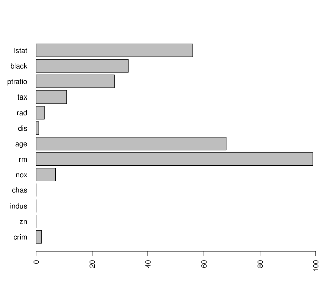
Figure 10: Number of times, each predictor in the Boston housing data set is significant at level $\alpha=0.05$ out of $100$ independent application of WGCM.est.

We see that the variable rm is almost always significant, and the variables age and lstat are significant in more than $50\%$ of the cases. These were also the significant variables for WGCM.est in the original analysis in Section 3.2.1. However, the analysis indicates that the $p$-values based on WGCM.est and hence also the number of significant variables is not very stable with respect to the randomness of the sample splitting. Depending on the split, it could well happen that only one or up to five variables are considered significant.

This leads to the question, how the $p$-values based on WGCM.est can be made more stable. Methods to aggregate $p$-values based on multiple sample splits have been developed in Meinshausen et al. (2009) and in DiCiccio et al. (2020). In the following, we apply the two approaches from Meinshausen et al. (2009) to the Boston housing data.

In the context of WGCM.est, let $B\in\mathbb{N}$.

1. Perform the test WGCM.est $B$ times with $B$ independent sample splits, obtaining $p$-values $P_{1},\ldots,P_{B}$.

2. For $\gamma\in(0,1)$, define the aggregated $p$-value $Q(\gamma)$ as

   $$Q(\gamma)=\min(1,q_{\gamma}(\{P_{b}/\gamma|b=1,\ldots,B\})),$$

   where $q_{\gamma}(\cdot)$ is the empirical $\gamma$-quantile.

If the $p$-values $P_{1},\ldots,P_{B}$ are asymptotically correct, then $Q(\gamma)$ is also an asymptotically correct $p$-value, see Theorem 3.1 Meinshausen et al. (2009).

However, one cannot simply search for $\gamma$ yielding the lowest value of $Q(\gamma)$. Instead, for a fixed lower bound $\gamma_{\text{min}}\in(0,1)$ define

$$P=\min\left(1,(1-\log\gamma_{\text{min}})\inf_{\gamma\in(\gamma_{\text{min}},1)}Q(\gamma)\right).$$

This is also an asymptotically correct $p$-value, see Theorem 3.2 in Meinshausen et al. (2009).

For the Boston housing data set, we again apply the procedure from Section 3.2.1 for $100$ independent splits of the sample, but without applying Holm’s method. For each of the $13$ predictors, we calculate the corresponding aggregated $p$-values $Q(\gamma)$ with $\gamma=\frac{1}{2}$ (Method 1) and $P$ with $\gamma_{\text{min}}=0.05$ (Method 2). At the end, we apply Holm’s correction once to the $13$ $p$-values from Method 1 and once to the $13$ $p$-values from Method 2. Plots of the $p$-values based on this procedure can be found in Figure 11. We see that for both aggregation methods, still the variables rm, age and lstat are significant.

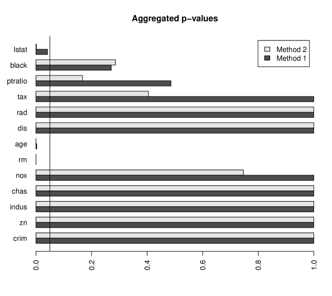
Figure 11: Aggregated $p$-values for the Boston housing data set using Method 1 and Method 2 based on $100$ independent applications of WGCM.est. Note that the results are comparable to Figure 7.

In principle, applying WGCM.est with multiple sample splits is a good idea, as it makes the $p$-values more stable. A caveat is however that especially in these variable importance examples, the runtime gets quite big, as there are already many tests involved in the procedure, even if only one sample split is used.

C Proofs of Section 2.2

In this section, we give the proofs of the Theorems on the univariate WGCM with single fixed and single estimated weight function.

C.1 A More General Result

To prove Theorem 1, we use the following more general result. Let $\mathcal{P}\subset\mathcal{P}_{0}$. For $P\in\mathcal{P}$ and $C,c>0$, define

$$\mathcal{W}_{P,C,c}=\left\{w:\mathbb{R}^{d_{Z}}\to\mathbb{R}\,\Bigr{\rvert}\,|w|\leq C\land\mathbb{E}_{P}\left[\epsilon_{P}^{2}\xi_{P}^{2}w(Z)^{2}\right]\geq c\right\}.$$

To be more precise, $\mathcal{W}_{P,C,c}$ is the set of measurable functions with those properties. For each $w\in\mathcal{W}_{P,C,c}$, let

$$R_{i}^{(n)}=R_{w,i}^{(n)}=\left(x_{i}-\hat{f}^{(n)}(z_{i})\right)\left(y_{i}-\hat{g}^{(n)}(z_{i})\right)w(z_{i}),\quad i=1,\ldots,n,$$

and let

$$T^{(n)}=T_{w}^{(n)}=\frac{\frac{1}{\sqrt{n}}\sum_{i=1}^{n}R_{i}^{(n)}}{\left(\frac{1}{n}\sum_{i=1}^{n}{\left(R_{i}^{(n)}\right)}^{2}-\left(\frac{1}{n}\sum_{r=1}^{n}R_{r}^{(n)}\right)^{2}\right)^{1/2}}=\frac{\tau_{N}^{(n)}}{\tau_{D}^{(n)}}.$$ (27)

Then, we have the following result under the null hypothesis:

Theorem 17

Let $A_{f}$, $A_{g}$, $B_{f}$ and $B_{g}$ be defined as in (11) and (12). Let $\mathcal{P}\subset\mathcal{P}_{0}$ and $C,c>0$. Assume that $A_{f}A_{g}=o_{\mathcal{P}}(n^{-1})$, $B_{f}=o_{\mathcal{P}}(1)$ and $B_{g}=o_{\mathcal{P}}(1)$. If there exists $\eta>0$ such that $\sup_{P\in\mathcal{P}}\mathbb{E}_{P}\left[|\epsilon_{P}\xi_{P}|^{2+\eta}\right]<\infty$, and if for all $P\in\mathcal{P}$, the set $\mathcal{W}_{P,C,c}$ is nonempty, then

$$\sup_{P\in\mathcal{P}}\sup_{w\in\mathcal{W}_{P,C,c}}\sup_{t\in\mathbb{R}}|\mathbb{P}_{P}(T_{w}^{(n)}\leq t)-\Phi(t)|\to 0.$$

We also have a more general power result. Let $\mathcal{P}\subset\mathcal{E}_{0}$. For $P\in\mathcal{P}$ and $C,c>0$, let

$$\mathcal{W}_{P,C,c}=\left\{w:\mathbb{R}^{d_{Z}}\to\mathbb{R}\,\Bigr{\rvert}\,|w|\leq C\land\operatorname{var}_{P}\left(\epsilon_{P}\xi_{P}w(Z)\right)\geq c\right\}.$$

Theorem 18

Let $A_{f}$, $A_{g}$, $B_{f}$ and $B_{g}$ be defined as in (11) and (12), but with the difference that $\hat{f}$ and $\hat{g}$ have been estimated on an auxiliary data set which is independent of $(\mathbf{X}^{(n)},\mathbf{Y}^{(n)},\mathbf{Z}^{(n)})$. Let $\mathcal{P}\subset\mathcal{E}_{0}$ and $C,c>0$. Assume that $A_{f}A_{g}=o_{\mathcal{P}}(n^{-1})$, $B_{f}=o_{\mathcal{P}}(1)$ and $B_{g}=o_{\mathcal{P}}(1)$. If there exists $\eta>0$ such that $\sup_{P\in\mathcal{P}}\mathbb{E}_{P}\left[|\epsilon_{P}\xi_{P}|^{2+\eta}\right]<\infty$, and if for all $P\in\mathcal{P}$, the set $\mathcal{W}_{P,C,c}$ is nonempty, then

$$\sup_{P\in\mathcal{P}}\sup_{w\in\mathcal{W}_{P,C,c}}\sup_{t\in\mathbb{R}}\left|\mathbb{P}_{P}\left(\frac{\tau_{N}^{(n)}-\sqrt{n}\rho_{P,w}}{\tau_{D}^{(n)}}\leq t\right)-\Phi(t)\right|\to 0,$$

where

$$\rho_{P,w}=\mathbb{E}_{P}\left[\epsilon_{P}\xi_{P}w(Z)\right].$$

C.2 Proofs

We first prove Theorem 17 and then show that Theorem 1 follows from Theorem 17.

C.2.1 Proof of Theorem 17

Proof  The proof closely follows the proof of Theorem 6 in Section D.1 in the supplementary material of Shah and Peters (2020). We will sometimes omit the dependence on $n$ and $P$ in the notation. We will repeatedly use limit theorems from Appendix F

Fix $C,c>0$ and write $\mathcal{W}_{P}$ instead of $\mathcal{W}_{P,C,c}$. For $n\in\mathbb{N}$, $P\in\mathcal{P}$ and $w\in\mathcal{W}_{P}$, define

$$\sigma_{w}^{2}=\sigma_{P,w}^{2}=\mathbb{E}_{P}\left[\epsilon_{P}^{2}\xi_{P}^{2}w(Z)^{2}\right].$$

We first prove that

$$\sup_{P\in\mathcal{P}}\sup_{w\in\mathcal{W}_{P}}\sup_{t\in\mathbb{R}}\left|\mathbb{P}_{P}\left(\frac{\frac{1}{\sqrt{n}}\sum_{i=1}^{n}\epsilon_{i}\xi_{i}w(z_{i})}{\sigma_{w}}\leq t\right)-\Phi(t)\right|\to 0.$$

To simplify notation, we will abbreviate this in the following with

$$\frac{\frac{1}{\sqrt{n}}\sum_{i=1}^{n}\epsilon_{i}\xi_{i}w(z_{i})}{\sigma_{w}}\stackrel{{\scriptstyle\mathcal{D};\mathcal{P},\mathcal{W}}}{{\to}}\mathcal{N}(0,1).$$ (28)

This is an application of Lemma 31, where the random variable $\zeta$ corresponds to $\frac{\epsilon_{P}\xi_{P}w(Z)}{\sigma_{w}}$. Instead of the set $\mathcal{P}$ of distributions for $\zeta$ in Lemma 31, we look at the set of distributions determined by $(P,w)$ for $\frac{\epsilon_{P}\xi_{P}w(Z)}{\sigma_{w}}$ where $P$ varies in $\mathcal{P}$ and $w$ varies in $\mathcal{W}_{P}$. We have

$$\mathbb{E}_{P}\left[\frac{\epsilon_{P}\xi_{P}w(Z)}{\sigma_{w}}\right]=\mathbb{E}_{P}\left[\mathbb{E}_{P}[\epsilon_{P}|Y,Z]\xi_{P}w(Z)\right]/\sigma_{w}=0$$

and $\mathbb{E}_{P}[\epsilon_{P}^{2}\xi_{P}^{2}w(Z)^{2}/\sigma_{w}^{2}]=1$ as well as

$$\sup_{P,w}\mathbb{E}_{P}\left[\left|\frac{\epsilon_{P}\xi_{P}w(Z)}{\sigma_{w}}\right|^{2+\eta}\right]\leq\left(\frac{C}{\sqrt{c}}\right)^{2+\eta}\sup_{P\in\mathcal{P}}\mathbb{E}_{P}\left[|\epsilon_{P}\xi_{P}|^{2+\eta}\right]<\infty$$

by assumption, so the lemma implies (28).

In the following, we will repeatedly apply Lemmas 32, 33 and 34 over the class of distributions for $\frac{\epsilon_{P}\xi_{P}w(Z)}{\sigma_{w}}$ determined by $(P,w)$ in a similar fashion.

For $i=1,\ldots n$, define

$$\Delta f_{i} =f(z_{i})-\hat{f}(z_{i}),$$

$$\Delta g_{i} =g(z_{i})-\hat{g}(z_{i}).$$

We first prove that

$$\frac{\tau_{N}}{\sigma_{w}}\stackrel{{\scriptstyle\mathcal{D};\mathcal{P},\mathcal{W}}}{{\to}}\mathcal{N}(0,1).$$ (29)

Observe that

$$\tau_{N}=\frac{1}{\sqrt{n}}\sum_{i=1}^{n}R_{i} =\frac{1}{\sqrt{n}}\sum_{i=1}^{n}w(z_{i})(f(z_{i})-\hat{f}(z_{i})+\epsilon_{i})(g(z_{i})-\hat{g}(z_{i})+\xi_{i})$$

$$=(b+\nu_{f}+\nu_{g})+\frac{1}{\sqrt{n}}\sum_{i=1}^{n}w(z_{i})\epsilon_{i}\xi_{i},$$ (30)

with

$$b =\frac{1}{\sqrt{n}}\sum_{i=1}^{n}w(z_{i})\Delta f_{i}\Delta g_{i},$$

$$\nu_{f} =\frac{1}{\sqrt{n}}\sum_{i=1}^{n}w(z_{i})\xi_{i}\Delta f_{i},$$

$$\nu_{g} =\frac{1}{\sqrt{n}}\sum_{i=1}^{n}w(z_{i})\epsilon_{i}\Delta g_{i}.$$

In analogy to the notation of (28), we write for a sequence $(V_{n})_{n\in\mathbb{N}}$ of random variables depending on $w\in\mathcal{W}_{P}$,

$$V_{n}=o_{\mathcal{P},\mathcal{W}}(1)$$

if for all $\delta>0$,

$$\sup_{P\in\mathcal{P}}\sup_{w\in\mathcal{W}_{P}}\mathbb{P}_{P}(|V_{n}|>\delta)\to 0.$$

For $b$, by the Cauchy-Schwarz inequality,

$$|b|\leq C\frac{1}{\sqrt{n}}\sum_{i=1}^{n}|\Delta f_{i}\Delta g_{i}|\leq C\sqrt{n}\sqrt{A_{f}A_{g}}=o_{\mathcal{P},\mathcal{W}}(1),$$ (31)

since $C\sqrt{n}\sqrt{A_{f}A_{g}}$ is independent of $w\in\mathcal{W}_{P}$ and $A_{f}A_{g}=o_{\mathcal{P}}\left(n^{-1}\right)$ by assumption.

Next, we want to control $\nu_{f}$ and $\nu_{g}$. For $\nu_{g}$,

$$\mathbb{E}_{P}[\epsilon_{i}\Delta g_{i}|\mathbf{Y},\mathbf{Z}] =\mathbb{E}_{P}[\epsilon_{i}|\mathbf{Z}]\Delta g_{i}=0,$$

$$\mathbb{E}_{P}[\epsilon_{i}^{2}\Delta g_{i}^{2}|\mathbf{Y},\mathbf{Z}] =\mathbb{E}_{P}[\epsilon_{i}^{2}|\mathbf{Z}]\Delta g_{i}^{2}=\Delta g_{i}^{2}u(z_{i}).$$

Thus,

$$\mathbb{E}_{P}[\nu_{g}^{2}|\mathbf{Y},\mathbf{Z}] \leq C^{2}\frac{1}{n}\sum_{i=1}^{n}\mathbb{E}_{P}[\epsilon_{i}^{2}\Delta g_{i}^{2}|\mathbf{Y},\mathbf{Z}]+C^{2}\sum_{i\neq j}\mathbb{E}_{P}[\epsilon_{i}\Delta g_{i}\epsilon_{j}\Delta g_{j}|\mathbf{Y},\mathbf{Z}]$$

$$=C^{2}\frac{1}{n}\sum_{i=1}^{n}\Delta g_{i}^{2}u(z_{i})+C^{2}\sum_{i\neq j}\mathbb{E}_{P}[\epsilon_{i}\Delta g_{i}|\mathbf{Y},\mathbf{Z}]\mathbb{E}_{P}[\epsilon_{j}\Delta g_{j}|\mathbf{Y},\mathbf{Z}]$$

$$=C^{2}\frac{1}{n}\sum_{i=1}^{n}\Delta g_{i}^{2}u(z_{i})=C^{2}B_{g}=o_{\mathcal{P}}(1)$$

by assumption. Since $C^{2}B_{g}$ is independent of $w\in\mathcal{W}_{P}$, we get that

$$\mathbb{E}_{P}[\nu_{g}^{2}|\mathbf{Y},\mathbf{Z}]=o_{\mathcal{P},\mathcal{W}}(1).$$ (32)

Thus, for all $\epsilon>0$ using Markov’s inequality,

$$\mathbb{P}_{P}\left(\nu_{g}^{2}\geq\epsilon\right) =\mathbb{P}_{P}\left(\nu_{g}^{2}\land\epsilon\geq\epsilon\right)$$

$$\leq\epsilon^{-1}\mathbb{E}_{P}\left[\mathbb{E}_{P}\left[\nu_{g}^{2}\land\epsilon|\mathbf{Y},\mathbf{Z}\right]\right]$$

$$\leq\epsilon^{-1}\mathbb{E}_{P}\left[\mathbb{E}_{P}\left[\nu_{g}^{2}|\mathbf{Y},\mathbf{Z}\right]\land\epsilon\right].$$

Equation (32) and Lemma 34 applied to the variables $\mathbb{E}[\nu_{g}^{2}|\mathbf{Y},\mathbf{Z}]$ with distributions determined by $(P,w)$ therefore imply that $\nu_{g}=o_{\mathcal{P},\mathcal{W}}(1)$. Similarly, $\nu_{f}=o_{\mathcal{P},\mathcal{W}}(1)$.

By (30), we have

$$\frac{\tau_{N}}{\sigma_{w}} =\frac{b+\nu_{f}+\nu_{g}}{\sigma_{w}}+\frac{\frac{1}{\sqrt{n}}\sum_{i=1}^{n}w(z_{i})\epsilon_{i}\xi_{i}}{\sigma_{w}}.$$

Since $\sigma_{w}\geq\sqrt{c}$, the first term is $o_{\mathcal{P},\mathcal{W}}(1)$. By (28) and Lemma 33, 1., we get (29).

Next, we aim to prove

$$\frac{\tau_{D}}{\sigma_{w}}=1+o_{\mathcal{P},\mathcal{W}}(1).$$ (33)

For this, it is enough to prove

$$\frac{\tau_{D}^{2}}{\sigma_{w}^{2}}=1+o_{\mathcal{P},\mathcal{W}}(1),$$ (34)

by continuity of $t\mapsto\sqrt{t}$ at $t=1$.

Recall that

$$\tau_{D}^{2}=\frac{1}{n}\sum_{i=1}^{n}{R_{i}}^{2}-\left(\frac{1}{n}\sum_{r=1}^{n}R_{r}\right)^{2}.$$

Since by (29), $\frac{1}{\sqrt{n}\sigma_{w}}\sum_{i=1}^{n}R_{i}=\frac{\tau_{N}}{\sigma_{w}}\stackrel{{\scriptstyle\mathcal{D};\mathcal{P},\mathcal{W}}}{{\to}}\mathcal{N}(0,1)$, it follows that $\frac{1}{n\sigma_{w}}\sum_{i=1}^{n}R_{i}=o_{\mathcal{P},\mathcal{W}}(1)$. To prove (34), it therefore suffices to prove

$$\frac{\frac{1}{n}\sum_{i=1}^{n}R_{i}^{2}}{\sigma_{w}^{2}}=1+o_{\mathcal{P},\mathcal{W}}(1).$$ (35)

For this, write

$$|R_{i}^{2}-w(z_{i})^{2}\epsilon_{i}^{2}\xi_{i}^{2}| \leq|w(z_{i})^{2}(\epsilon_{i}+\Delta f_{i})^{2}(\xi_{i}+\Delta g_{i})^{2}-w(z_{i})^{2}\epsilon_{i}^{2}\xi_{i}^{2}|$$

$$\leq\underbrace{w(z_{i})^{2}(\Delta f_{i}^{2}+2|\epsilon_{i}\Delta f_{i}|)(\Delta g_{i}^{2}+2|\xi_{i}\Delta g_{i}|)}_{\eqqcolon I_{i}}$$

$$+\underbrace{w(z_{i})^{2}\epsilon_{i}^{2}(\Delta g_{i}^{2}+2|\xi_{i}\Delta g_{i}|)}_{\eqqcolon II_{i}}+\underbrace{w(z_{i})^{2}\xi_{i}^{2}(\Delta f_{i}^{2}+2|\epsilon_{i}\Delta f_{i}|)}_{\eqqcolon III_{i}}$$ (36)

For $I_{i}$, observe that $2\Delta f_{i}^{2}|\xi_{i}\Delta g_{i}|\leq\Delta f_{i}^{2}(\xi_{i}^{2}+\Delta g_{i}^{2})$ and $2\Delta g_{i}^{2}|\epsilon_{i}\Delta f_{i}|\leq\Delta g_{i}^{2}(\epsilon_{i}^{2}+\Delta f_{i}^{2})$. Thus, we have

$$I_{i} \leq C^{2}(\Delta f_{i}^{2}\Delta g_{i}^{2}+2\Delta f_{i}^{2}|\xi_{i}\Delta g_{i}|+2\Delta g_{i}^{2}|\epsilon_{i}\Delta f_{i}|+4|\epsilon_{i}\xi_{i}\Delta f_{i}\Delta g_{i}|)$$

$$\leq C^{2}(3\Delta f_{i}^{2}\Delta g_{i}^{2}+\epsilon_{i}^{2}\Delta g_{i}^{2}+\xi_{i}^{2}\Delta f_{i}^{2}+4|\epsilon_{i}\xi_{i}\Delta f_{i}\Delta g_{i}|).$$

Observe that

$$\frac{1}{n}\sum_{i=1}^{n}\Delta f_{i}^{2}\Delta g_{i}^{2}\leq\frac{1}{n}\sum_{i=1}^{n}\Delta f_{i}^{2}\sum_{i=1}^{n}\Delta g_{i}^{2}=nA_{f}A_{g}=o_{\mathcal{P}}(1)$$

by assumption. Furthermore, for all $\delta>0$

$$\mathbb{P}_{P}\left(\frac{1}{n}\sum_{i=1}^{n}\epsilon_{i}^{2}\Delta g_{i}^{2}\geq\delta\right) =\mathbb{P}_{P}\left(\frac{1}{n}\sum_{i=1}^{n}\epsilon_{i}^{2}\Delta g_{i}^{2}\wedge\delta\geq\delta\right)$$

$$\leq\delta^{-1}\mathbb{E}_{P}\left[\mathbb{E}_{P}\left[\frac{1}{n}\sum_{i=1}^{n}\epsilon_{i}^{2}\Delta g_{i}^{2}\wedge\delta|\mathbf{Y},\mathbf{Z}\right]\right]$$

$$\leq\delta^{-1}\mathbb{E}_{P}\left[\mathbb{E}_{P}\left[\frac{1}{n}\sum_{i=1}^{n}\epsilon_{i}^{2}\Delta g_{i}^{2}|\mathbf{Y},\mathbf{Z}\right]\wedge\delta\right]$$

$$=\delta^{-1}\mathbb{E}_{P}\left[B_{g}\wedge\delta\right],$$

similarly as before. Since $B_{g}=o_{\mathcal{P}}(1)$ by assumption, Lemma 34 implies that $\mathbb{E}_{P}[B_{g}\land\delta]\to 0$ and thus,

$$\frac{1}{n}\sum_{i=1}^{n}\epsilon_{i}^{2}\Delta g_{i}^{2}=o_{\mathcal{P}}(1).$$ (37)

Similarly, also $n^{-1}\sum_{i=1}^{n}\xi_{i}^{2}\Delta f_{i}^{2}=o_{\mathcal{P}}(1)$. Moreover,

$$\frac{1}{n}\sum_{i=1}^{n}|\epsilon_{i}\xi_{i}\Delta f_{i}\Delta g_{i}| \leq\left(\frac{1}{n}\sum_{i=1}^{n}\epsilon_{i}^{2}\xi_{i}^{2}\right)^{1/2}\left(\frac{1}{n}\sum_{i=1}^{n}\Delta f_{i}^{2}\Delta g_{i}^{2}\right)^{1/2}$$

$$\leq\left(\frac{1}{n}\sum_{i=1}^{n}\epsilon_{i}^{2}\xi_{i}^{2}\right)^{1/2}\left(\frac{1}{n}\sum_{i=1}^{n}\Delta f_{i}^{2}\sum_{i=1}^{n}\Delta g_{i}^{2}\right)^{1/2}$$ (38)

By Lemma 32, we have that for all $\delta>0$

$$\sup_{P\in\mathcal{P}}\mathbb{P}_{P}\left(\left|\frac{1}{n}\sum_{i=1}^{n}\epsilon_{i}^{2}\xi_{i}^{2}-\mathbb{E}_{P}[\epsilon^{2}\xi^{2}]\right|>\delta\right)\to 0,$$

so

$$\frac{1}{n}\sum_{i=1}^{n}\epsilon_{i}^{2}\xi_{i}^{2}=O_{\mathcal{P}}(1).$$ (39)

The second factor in (38) is equal to $\sqrt{nA_{f}A_{g}}=o_{\mathcal{P}}(1)$. This implies $n^{-1}\sum_{i=1}^{n}|\epsilon_{i}\xi_{i}\Delta f_{i}\Delta g_{i}|=o_{\mathcal{P}}(1)$. In total, we get

$$\frac{1}{n}\sum_{i=1}^{n}I_{i}=o_{\mathcal{P},\mathcal{W}}(1).$$ (40)

For $II_{i}$, we have

$$\frac{1}{n}\sum_{i=1}^{n}w(z_{i})^{2}(\epsilon_{i}^{2}\Delta g_{i}^{2}+2\epsilon_{i}^{2}|\xi_{i}\Delta g_{i}|) \leq 2C^{2}\left(\frac{1}{n}\sum_{i=1}^{n}\epsilon_{i}^{2}\xi_{i}^{2}\right)^{1/2}\left(\frac{1}{n}\sum_{i=1}^{n}\epsilon_{i}^{2}\Delta g_{i}^{2}\right)^{1/2}+\frac{C^{2}}{n}\sum_{i=1}^{n}\epsilon_{i}^{2}\Delta g_{i}^{2}.$$

By (37), $n^{-1}\sum_{i=1}^{n}\epsilon_{i}^{2}\Delta g_{i}^{2}=o_{\mathcal{P}}(1)$, so using (39), also

$$\frac{1}{n}\sum_{i=1}^{n}II_{i}=o_{\mathcal{P},\mathcal{W}}(1).$$

Similarly, $\frac{1}{n}\sum_{i=1}^{n}III_{i}=o_{\mathcal{P},\mathcal{W}}(1)$. Combining this with (40) and (36), we get

$$\frac{1}{n}\sum_{i=1}^{n}R_{i}^{2}=\frac{1}{n}\sum_{i=1}^{n}w(z_{i})^{2}\epsilon_{i}^{2}\xi_{i}^{2}+o_{\mathcal{P},\mathcal{W}}(1).$$

With Lemma 32, we obtain that for all $\delta>0$

$$\sup_{P\in\mathcal{P}}\sup_{w\in\mathcal{W}_{P}}\mathbb{P}_{P}\left(\left|\frac{1}{n}\sum_{i=1}^{n}w(z_{i})^{2}\epsilon_{i}^{2}\xi_{i}^{2}-\sigma_{w}^{2}\right|>\delta\right)\to 0$$

and thus,

$$\frac{1}{n}\sum_{i=1}^{n}R_{i}^{2}-\sigma_{w}^{2}=o_{\mathcal{P},\mathcal{W}}(1).$$

Since $\sigma_{w}^{2}\geq c$, we obtain

$$\frac{\frac{1}{n}\sum_{i=1}^{n}R_{i}^{2}}{\sigma_{w}^{2}}-1=o_{\mathcal{P},\mathcal{W}}(1)$$

so (35) and (33) follow. Since $T^{(n)}=\frac{\tau_{N}^{(n)}/\sigma_{w}}{\tau_{D}^{(n)}/\sigma_{w}}$, we get by Lemma 33 with (29)

$$T^{(n)}\stackrel{{\scriptstyle\mathcal{D};\mathcal{P},\mathcal{W}}}{{\to}}\mathcal{N}(0,1).$$

This concludes the proof.  

C.2.2 Proof of Theorem 1

Proof  The statement 2. follows from Theorem 17 in the following way: For $P\in\mathcal{P}$, $w\in\mathcal{W}_{P,C,c}$ and $t\in\mathbb{R}$, let

$$\Gamma_{n}(P,w,t)=\mathbb{P}_{P}(T_{w}^{(n)}\leq t).$$

with $T_{w}^{(n)}$ defined as in (27). By Theorem 17, we have

$$\sup_{P\in\mathcal{P}}\sup_{w\in\mathcal{W}_{P,C,c}}\sup_{t\in\mathbb{R}}|\Gamma_{n}(P,w,t)-\Phi(t)|\to 0.$$

For the auxiliary data set $\mathbf{A}$, let $\left(\hat{w}^{(n)}\right)_{n\in\mathbb{N}}$ be the sequence of functions estimated on $\mathbf{A}$. From the assumptions of Theorem 1, 2., we know that there exist $C,c>0$ such that for all $P\in\mathcal{P}$, $P$-almost surely for all $n\in\mathbb{N}$ we have $\hat{w}^{(n)}\in\mathcal{W}_{P,C,c}$. Since $\mathbf{A}$ is independent of $(\mathbf{X}^{(n)},\mathbf{Y}^{(n)},\mathbf{Z}^{(n)})$, we have

$$\mathbb{P}_{P}(T^{(n)}\leq t|\mathbf{A})=\Gamma_{n}(P,\hat{w}^{(n)},t).$$

Using iterated expectations, it follows that

$$\sup_{P\in\mathcal{P}}\sup_{t\in\mathbb{R}}\left|\mathbb{P}_{P}(T^{(n)}\leq t)-\Phi(t)\right| =\sup_{P\in\mathcal{P}}\sup_{t\in\mathbb{R}}\left|\mathbb{E}_{P}\left[\Gamma_{n}(P,\hat{w}^{(n)},t)\right]-\Phi(t)\right|$$

$$\leq\sup_{P\in\mathcal{P}}\mathbb{E}_{P}\left[\sup_{t\in\mathbb{R}}|\Gamma_{n}(P,\hat{w}^{(n)},t)-\Phi(t)|\right]$$

$$\leq\sup_{P\in\mathcal{P}}\mathbb{E}_{P}\left[\sup_{Q\in\mathcal{P}}\sup_{w\in\mathcal{W}_{Q,C,c}}\sup_{t\in\mathbb{R}}|\Gamma_{n}(Q,w,t)-\Phi(t)|\right]$$

$$=\sup_{P\in\mathcal{P}}\sup_{w\in\mathcal{W}_{P,C,c}}\sup_{t\in\mathbb{R}}|\Gamma_{n}(P,w,t)-\Phi(t)|\to 0.$$

This concludes the proof of 2. The statement 1. can be proven in a similar fashion, but since we do not require uniformity over a collection $\mathcal{P}$, it is enough to have

$$\mathbb{P}_{P}(T^{(n)}\leq t|\mathbf{A})\to\Phi(t)\text{ a.s.}$$ (41)

Then, one can conclude using dominated convergence. To show (41), it is enough to a.s. have $c>0$ such that $\sigma_{n}^{2}\geq c$, so $c$ is allowed to depend on $\mathbf{A}$.  

C.2.3 Proof of Theorem 18

Proof  The proof is very similar to the proof of Theorem 17, see also the proof of Theorem 8 in Section D.3 in the supplementary material of Shah and Peters (2020). We will therefore only sketch the main steps. Apart from not assuming the null hypothesis anymore, a main difference is that we have a data set $\mathbf{B}$ independent of $(\mathbf{X}^{(n)},\mathbf{Y}^{(n)},\mathbf{Z}^{(n)})$ on which $\hat{f}$ and $\hat{g}$ have been estimated.

Let

$$\rho_{w}=\rho_{P,w}=\mathbb{E}_{P}[\epsilon_{P}\xi_{P}w(Z)]$$

and

$$\sigma_{w}^{2}=\sigma_{P,w}^{2}=\operatorname{var}_{P}(\epsilon_{P}\xi_{P}w(Z))=\mathbb{E}_{P}\left[\epsilon_{P}^{2}\xi_{P}^{2}w(Z)^{2}\right]-\rho_{P,w}^{2}.$$

We first prove that (with the notation of (28) and (29))

$$\frac{\tau_{N}-\sqrt{n}\rho_{w}}{\sigma_{w}}\stackrel{{\scriptstyle\mathcal{D};\mathcal{P},\mathcal{W}}}{{\to}}\mathcal{N}(0,1).$$ (42)

For this, write

$$\tau_{N}-\sqrt{n}\rho_{w} =(b+\nu_{f}+\nu_{g})+\frac{1}{\sqrt{n}}\sum_{i=1}^{n}\left(\epsilon_{i}\xi_{i}w(z_{i})-\rho_{w}\right),$$ (43)

with $b$, $\nu_{f}$ and $\nu_{g}$ defined as in (30). Similarly to (28), one can show that

$$\frac{1}{\sqrt{n}\sigma_{w}}\sum_{i=1}^{n}\left(\epsilon_{i}\xi_{i}w(z_{i})-\rho_{w}\right)\stackrel{{\scriptstyle\mathcal{D};\mathcal{P},\mathcal{W}}}{{\to}}\mathcal{N}(0,1).$$

The term $b$ can be controlled as in (31). For the term $\nu_{g}$, replace conditioning on $\mathbf{Y},\mathbf{Z}$ by conditioning on $\mathbf{B},\mathbf{Z}$ and similarly for $\nu_{f}$. Since $\sigma_{w}^{2}\geq c$, we arrive at (42).

Next, we prove

$$\frac{\tau_{D}}{\sigma_{w}}=1+o_{\mathcal{P},\mathcal{W}}(1),$$ (44)

which follows from ${\tau_{D}^{2}}/{\sigma_{w}^{2}}=1+o_{\mathcal{P},\mathcal{W}}(1).$ Recall that

$$\tau_{D}^{2}=\frac{1}{n}\sum_{i=1}^{n}{R_{i}}^{2}-\left(\frac{1}{n}\sum_{r=1}^{n}R_{r}\right)^{2}.$$ (45)

Since by (42), $\frac{1}{\sqrt{n}\sigma_{w}}\sum_{i=1}^{n}(R_{i}-\rho_{w})\stackrel{{\scriptstyle\mathcal{D};\mathcal{P},\mathcal{W}}}{{\to}}\mathcal{N}(0,1)$, we have

$$\frac{\frac{1}{n}\sum_{i=1}^{n}R_{i}-\rho_{w}}{\sigma_{w}}=o_{\mathcal{P},\mathcal{W}}(1).$$ (46)

Next, we show

$$\frac{\frac{1}{n}\sum_{i=1}^{n}R_{i}^{2}-\mathbb{E}_{P}\left[\epsilon^{2}\xi^{2}w(Z)^{2}\right]}{\sigma_{w}^{2}}=o_{\mathcal{P},\mathcal{W}}(1).$$ (47)

For this, write

$$|R_{i}^{2}-w(z_{i})^{2}\epsilon_{i}^{2}\xi_{i}^{2}|\leq I_{i}+II_{i}+III_{i}$$

exactly as in the proof of Theorem 17. By replacing conditioning on $\mathbf{Y},\mathbf{Z}$ with conditioning on $\mathbf{B},\mathbf{Z}$, one can show

$$\sum_{i=1}^{n}(I_{i}+II_{i}+III_{i})=o_{\mathcal{P},\mathcal{W}}(1)$$

in the same way as there. Using Lemma 32, one can show

$$\frac{1}{n}\sum_{i=1}^{n}\epsilon_{i}^{2}\xi_{i}^{2}w(z_{i})^{2}-\mathbb{E}_{P}[\epsilon^{2}\xi^{2}w(Z)^{2}]=o_{\mathcal{P},\mathcal{W}}(1),$$

so this implies (47).

Equations (45), (46) and (47) together imply

$$\frac{\tau_{D}^{2}}{\sigma_{w}^{2}} =\frac{\mathbb{E}_{P}[\epsilon^{2}\xi^{2}w(Z)^{2}]}{\sigma_{w}^{2}}+o_{\mathcal{P},\mathcal{W}}(1)-\left(\frac{\rho_{w}}{\sigma_{w}}+o_{\mathcal{P},\mathcal{W}}(1)\right)^{2}$$

$$=\frac{\mathbb{E}_{P}[\epsilon^{2}\xi^{2}w(Z)^{2}]-\rho_{w}^{2}}{\sigma_{w}^{2}}+o_{\mathcal{P},\mathcal{W}}(1)$$

$$=1+o_{\mathcal{P},\mathcal{W}}(1),$$

where we used that $|\rho_{w}|$ is bounded in the second line. Thus, we get (44) and can conclude using Lemma 33.  

C.2.4 Proof of Theorem 3

Proof  Proving Theorem 3 can be reduced to Theorem 18, just as Theorem 1 could be reduced to Theorem 17.  

D Proof of Theorem 8

To prove Theorem 8, we use the strategy of the proof of Theorem 9 in Section D.4 of Shah and Peters (2020). We will heavily rely on results from Chernozhukov et al. (2013), which we summarise in the following.

D.1 Summary of Results on Gaussian Approximation of Maxima of Random Vectors

We present the following results in the form they are also presented in Section D.4.1 in Shah and Peters (2020), which are sometimes special cases of the corresponding results in Chernozhukov et al. (2013). There is the following difference to the results given there: We consider maxima of absolute values of random vectors instead of maxima of random vectors. The results for the maxima translate to the corresponding results for the absolute value by considering the vector $(Y,-Y)$ instead of just the vector $Y$.

Assume $W\sim\mathcal{N}_{p}(0,\Sigma)$, with $\Sigma_{jj}=1$ for $j=1,\ldots,p$. Assume $p\geq 3$ possibly depending on $n$. Let $V=\max_{j=1,\ldots,p}|W_{j}|$. Let $\tilde{W}$ be a random vector taking values in $\mathbb{R}^{p}$ with $\mathbb{E}[\tilde{W}]=0$ and $\operatorname{Cov}(\tilde{W})=\Sigma$ and let $\tilde{w}_{1},\ldots,\tilde{w}_{n}\in\mathbb{R}^{p}$ be i.i.d copies of $\tilde{W}$. Let

$$\tilde{V}=\max_{j=1,\ldots,p}\left|\frac{1}{\sqrt{n}}\sum_{i=1}^{n}\tilde{w}_{ij}\right|,$$

where $\tilde{w}_{ij}$ is the $j$th component of $\tilde{w}_{i}$. We need the following conditions for some sequence $(B_{n})_{n\in\mathbb{N}}$ with $B_{n}\geq 1$:

• $\max_{k=1,2}\mathbb{E}\left[|\tilde{W}_{j}|^{2+k}/B_{n}^{k}\right]+\mathbb{E}\left[\exp\left(|\tilde{W}_{j}|/B_{n}\right)\right]\leq 4$ for all $j=1,\ldots,p$;

• $\max_{k=1,2}\mathbb{E}\left[|\tilde{W}_{j}|^{2+k}/B_{n}^{k/2}\right]+\mathbb{E}\left[\max_{j=1,\ldots,p}|\tilde{W}_{j}|^{4}/B_{n}^{2}\right]\leq 4$ for all $j=1,\ldots,p$;

• There exist some constants $C_{1},c_{1}>0$ such that $B_{n}^{2}\left(\log(pn)\right)^{7}/n\leq C_{1}n^{-c_{1}}$.

The following Lemma corresponds to Corollary 2.1 in Chernozhukov et al. (2013) and Theorem 22 in Shah and Peters (2020):

Lemma 19

Assume that either (B1a) and (B2) or (B1b) and (B2) hold. Then, there exist constants $c,C>0$ depending only on $c_{1}$ and $C_{1}$ such that

$$\sup_{t\in\mathbb{R}}|\mathbb{P}(\tilde{V}\leq t)-\mathbb{P}(V\leq t)|\leq Cn^{-c}.$$

The next Lemma corresponds to Lemma 24 in Shah and Peters (2020) and follows from Lemma C.1 in Section C.5 of Chernozhukov et al. (2013) (first statement) and is an application of Lemma A.1 in Section A.1 there (second statement).

Lemma 20

Again assume that either (B1a) and (B2) or (B1b) and (B2) hold. Let $\tilde{\Sigma}=\sum_{i=1}^{n}\tilde{w}_{i}\tilde{w}_{i}^{T}/n$ be the empirical covariance matrix of $\tilde{w}_{1},\ldots,\tilde{w}_{n}$. Then, there exist constants $c,C$ depending only on $C_{1}$ and $c_{1}$ such that

$$\log(p)^{2}\mathbb{E}\left[\|\tilde{\Sigma}-\Sigma\|_{\infty}\right] \leq Cn^{-c}$$

$$\log(p)^{2}\mathbb{E}\left[\max_{j=1,\ldots,p}\left|\frac{1}{n}\sum_{i=1}^{n}\tilde{w}_{ij}\right|\right] \leq Cn^{-c}.$$

The following lemma corresponds to Lemma 2.1 in Chernozhukov et al. (2013) and to Lemma 21 in Shah and Peters (2020).

Lemma 21

Let $W=(W_{1},\ldots,W_{p})^{T}$ have a multivariate Gaussian distribution with $\mathbb{E}[W_{i}]=0$ and $\mathbb{E}[W_{i}^{2}]=1$ for all $i=1,\ldots,p$. Then, there exists a universal constant $C>0$ such that for all $t\geq 0$

$$\sup_{w\geq 0}\mathbb{P}\left(\left|\max_{j=1,\ldots,p}|W_{j}|-w\right|\leq t\right)\leq Ct\left(\sqrt{2\log(p)}+1\right).$$

Define the function

$$q(\theta)=\theta^{1/3}(2\lor\log(p/\theta))^{2/3}.$$

One may check by differentiating that $q$ is increasing in $\theta$. The following Lemma corresponds to Lemma 3.1 in Chernozhukov et al. (2013) and to Lemma 23 in Shah and Peters (2020).

Lemma 22

Let $U$ and $W$ be centered multivariate Gaussian random vectors taking values in $\mathbb{R}^{p}$. Let $U$ have covariance matrix $\Theta$ and $W$ have covariance matrix $\Sigma$, such that for $i=1,\ldots,p$, we have $\Sigma_{ii}=1$. Let $\Delta_{0}=\max_{j,k=1,\ldots,p}|\Sigma_{jk}-\Theta_{jk}|$. Then, there exists a universal constant $C>0$ such that

1. $\sup_{t\in\mathbb{R}}|\mathbb{P}\left(\max_{j=1,\ldots,p}|U_{j}|\leq t\right)-\mathbb{P}\left(\max_{j=1,\ldots,p}|W_{j}|\leq t\right)|\leq Cq(\Delta_{0}).$

2. Let $G_{\Sigma}$ and $G_{\Theta}$ be the quantile functions of $\max_{j=1,\ldots,p}|W_{j}|$ and $\max_{j=1,\ldots,p}|U_{j}|$. Then, for all $\alpha\in(0,1)$

   $$G_{\Theta}(\alpha)\leq G_{\Sigma}(\alpha+Cq(\Delta_{0}))\quad\text{and}\quad G_{\Sigma}(\alpha)\leq G_{\Theta}(\alpha+Cq(\Delta_{0})).$$

Note that 2. follows from 1. by observing that

$$\mathbb{P}\left(\max_{j}|U_{j}|\leq G_{\Sigma}\left(\alpha+Cq(\Delta_{0})\right)\right)\stackrel{{\scriptstyle 1.}}{{\geq}}\mathbb{P}\left(\max_{j}|W_{j}|\leq G_{\Sigma}\left(\alpha+Cq(\Delta_{0})\right)\right)-Cq(\Delta_{0})=\alpha,$$

so $G_{\Theta}(\alpha)\leq G_{\Sigma}\left(\alpha+Cq(\Delta_{0})\right)$. Similarly, the second statement of 2. follows.

D.2 Proof of Theorem 8

We prove a slightly more general result, similar to Section C.1, since we later also want to apply a version of this theorem and its proof to estimated weight functions, see Appendix E.

For $P\in\mathcal{P}$ and $C,c>0$, define

$$\mathcal{W}_{P,C,c}=\left\{w:\mathbb{R}^{d_{Z}}\to\mathbb{R}\,\Bigr{\rvert}\,|w|\leq C\land\mathbb{E}_{P}\left[\epsilon_{P}^{2}\xi_{P}^{2}w(Z)^{2}\right]\geq c\right\}.$$

For $\mathbf{w}=(w_{1},\ldots,w_{K})^{T}\in\mathcal{W}_{P,C,c}^{K}$, let $S_{n,\mathbf{w}}$ and $\hat{G}_{n,\mathbf{w}}$ be the versions of $S_{n}$ and $\hat{G}_{n}$ based on $\mathbf{w}=(w_{1},\ldots,w_{K})^{T}$.

Theorem 23

Let $\mathcal{P}\subset\mathcal{P}_{0}$ and let $A_{f}$, $A_{g}$, $B_{f}$ and $B_{g}$ be defined as in (11) and (12). Assume that there exist $C,c\geq 0$ such that for all $n\in\mathbb{N}$ and $P\in\mathcal{P}$ there exists $B\geq 1$ such that either (A1a) and (A2) or (A1b) and (A2) hold. Let $C_{1},c_{1}>0$ such that for all $P\in\mathcal{P}$ the set $\mathcal{W}_{P,C_{1},c_{1}}$ is not empty. Assume that

$$A_{f}A_{g}=o_{\mathcal{P}}\left(n^{-1}\log(K)^{-2}\right),$$ (48)

$$B_{f}=o_{\mathcal{P}}\left(\log(K)^{-4}\right),\quad B_{g}=o_{\mathcal{P}}\left(\log(K)^{-4}\right).$$ (49)

Assume that there exist sequences $\left(\tau_{f,n}\right)_{n\in\mathbb{N}}$ and $\left(\tau_{g,n}\right)_{n\in\mathbb{N}}$ such that

$$\max_{i=1,\ldots,n}|\epsilon_{P,i}|=O_{\mathcal{P}}(\tau_{g,n}),\quad A_{g}=o_{\mathcal{P}}\left(\tau_{g,n}^{-2}\log(K)^{-2}\right),$$ (50)

$$\max_{i=1,\ldots,n}|\xi_{P,i}|=O_{\mathcal{P}}(\tau_{f,n}),\quad A_{f}=o_{\mathcal{P}}\left(\tau_{f,n}^{-2}\log(K)^{-2}\right).$$ (51)

Then,

$$\sup_{P\in\mathcal{P}}\sup_{\mathbf{w}\in\mathcal{W}_{P,C_{1},c_{1}}^{K}}\sup_{\alpha\in(0,1)}|\mathbb{P}_{P}(S_{n,\mathbf{w}}\leq\hat{G}_{n,\mathbf{w}}(\alpha))-\alpha|\to 0.$$

We see that Theorem 8 follows from Theorem 23.

Proof [Proof of Theorem 23] We closely follow Section D.4.2 in Shah and Peters (2020). In the following, we will often omit dependencies on $P$, $\mathbf{w}$ and $n$ and we will often write $x\lesssim y$ instead of there exists a constant $C>0$ independent of $n$, $P$ and $\mathbf{w}$ such that $x\leq Cy$.

Fix $C_{1},c_{1}>0$ and write $\mathcal{W}_{P}=\mathcal{W}_{P,C_{1},c_{1}}$. For $P\in\mathcal{P}$, $\mathbf{w}=(w_{1},\ldots,w_{K})^{T}\in\mathcal{W}_{P}^{K}$ and $k=1,\ldots,K$ let

$$\sigma_{k}^{2}=\sigma_{P,\mathbf{w},k}^{2}=\mathbb{E}_{P}[\epsilon_{P}^{2}\xi_{P}^{2}w_{k}(Z)^{2}].$$

We have for all $k=1,\ldots,K$

$$\mathbb{E}_{P}[\epsilon\xi w_{k}(Z)]=\mathbb{E}_{P}[\mathbb{E}_{P}[\epsilon|Z,Y]\xi w_{k}(Z)]=0.$$

We will need the conditions (B1a)/(B1b) and (B2) to hold for the random vectors

$$\left\{\left(\frac{\epsilon_{i}\xi_{i}w_{k}(z_{i})}{\sigma_{k}}\right)_{k=1}^{K}\right\}_{i=1}^{n}.$$

This is guaranteed by (A1a)/(A1b) and (A2), since

$$|w_{k}(z_{i})/\sigma_{k}|\leq C_{1}/\sqrt{c_{1}}\eqqcolon\gamma.$$

Consider the definition (13) of $T_{k}^{(n)}$. Write $\tau_{N,k}^{(n)}/\sigma_{k}=\sqrt{n}\bar{\mathbf{R}}_{k}/\sigma_{k}=\delta_{k}+\tilde{T}_{k}$ with

$$\tilde{T}_{k}=\frac{1}{\sqrt{n}}\sum_{i=1}^{n}\frac{\epsilon_{i}\xi_{i}w_{k}(z_{i})}{\sigma_{k}}.$$

Write

$$\frac{\tau_{D,k}^{(n)}}{\sigma_{k}}=\frac{\left(\frac{1}{n}\|\mathbf{R}_{k}\|_{2}^{2}-\bar{\mathbf{R}}_{k}^{2}\right)^{1/2}}{\sigma_{k}}=1+\Delta_{k}.$$

It follows that

$$T_{k}=\frac{\tilde{T}_{k}+\delta_{k}}{1+\Delta_{k}}.$$

Define $\tilde{S}_{n}=\max_{k=1,\ldots,K}|\tilde{T}_{k}|$ and define the matrix $\Sigma\in\mathbb{R}^{K\times K}$ by

$$\Sigma_{kl}=\frac{\mathbb{E}_{P}[\epsilon^{2}\xi^{2}w_{k}(Z)w_{l}(Z)]}{\sigma_{k}\sigma_{l}}.$$

Note that the diagonal of $\Sigma$ consists of ones. Let $W=(W_{1},\ldots,W_{K})^{T}$ be a random vector with distribution $\mathcal{N}_{K}(0,\Sigma)$. Let $V_{n}=\max_{k=1,\ldots,K}|W_{k}|$ and let $G_{n}$ be the quantile function of $V_{n}$. Note that $\Sigma$, $W$, $V_{n}$ and $G_{n}$ all depend on $P$ and $\mathbf{w}$. Lemma 21 implies that the distribution function of $V_{n}$ is continuous, so for all $\alpha\in[0,1]$, we have $\mathbb{P}_{P}(V_{n}\leq G_{n}(\alpha))=\alpha$. Our goal is to bound

$$v_{P,\mathbf{w}}(\alpha)=|\mathbb{P}_{P}(S_{n,\mathbf{w}}\leq\hat{G}_{n,\mathbf{w}}(\alpha))-\alpha|.$$

For this, define

$$\kappa_{P,\mathbf{w}}=\sup_{t\in\mathbb{R}}|\mathbb{P}_{P}(S_{n,\mathbf{w}}\leq t)-\mathbb{P}_{P}(V_{n}\leq t)|.$$

Fix $P\in\mathcal{P}$ and $\mathbf{w}\in\mathcal{W}_{P}$. Let $\triangle$ denote the symmetric difference. Using the triangle inequality and $|\mathbb{P}(A)-\mathbb{P}(B)|\leq\mathbb{P}(A\triangle B)$, we have

$$v(\alpha) \leq|\mathbb{P}(S_{n}\leq\hat{G}_{n}(\alpha))-\mathbb{P}(S_{n}\leq G_{n}(\alpha))|+|\mathbb{P}(S_{n}\leq G_{n}(\alpha))-\mathbb{P}(V_{n}\leq G_{n}(\alpha))|$$

$$\leq\mathbb{P}(\{S_{n}\leq\hat{G}_{n}(\alpha)\}\triangle\{S_{n}\leq G_{n}(\alpha)\})+\kappa.$$

Let $u_{\Sigma}>0$. By Lemma 22, $\|\Sigma-\hat{\Sigma}\|_{\infty}\leq u_{\Sigma}$ implies $G_{n}(\alpha-C^{\prime}q(u_{\Sigma}))\leq\hat{G}_{n}(\alpha)\leq G_{n}(\alpha+C^{\prime}q(u_{\Sigma}))$. This means that if $\|\Sigma-\hat{\Sigma}\|_{\infty}\leq u_{\Sigma}$, we have that $G_{n}(\alpha)<S_{n}\leq\hat{G}_{n}(\alpha)$ implies $G_{n}(\alpha)<S_{n}\leq G_{n}(\alpha+C^{\prime}q(u_{\Sigma}))$ and $\hat{G}_{n}(\alpha)<S_{n}\leq G_{n}(\alpha)$ implies $G_{n}(\alpha-C^{\prime}q(u_{\Sigma}))\leq S_{n}\leq G_{n}(\alpha)$. We obtain

$$\mathbb{P}\left(\{S_{n}\leq\hat{G}_{n}(\alpha)\}\triangle\{S_{n}\leq G_{n}(\alpha)\}\right)$$

$$\leq\mathbb{P}\left(G_{n}(\alpha-C^{\prime}q(u_{\Sigma}))\leq S_{n}\leq G_{n}(\alpha+C^{\prime}q(u_{\Sigma}))\right)+\mathbb{P}(\|\Sigma-\hat{\Sigma}\|_{\infty}>u_{\Sigma})$$

$$\leq 2\kappa+\mathbb{P}(G_{n}(\alpha-C^{\prime}q(u_{\Sigma}))\leq V_{n}\leq G_{n}(\alpha+C^{\prime}q(u_{\Sigma})))+\mathbb{P}(\|\Sigma-\hat{\Sigma}\|_{\infty}>u_{\Sigma})$$

$$=2\kappa+2C^{\prime}q(u_{\Sigma})+\mathbb{P}(\|\Sigma-\hat{\Sigma}\|_{\infty}>u_{\Sigma}).$$

In total, we obtain

$$v(\alpha)\lesssim\kappa+q(u_{\Sigma})+\mathbb{P}(\|\Sigma-\hat{\Sigma}\|_{\infty}>u_{\Sigma}).$$

For $0<u_{\delta},u_{\Delta}\leq 1$, define the event $\Omega=\{\max_{k=1,\ldots,K}|\delta_{k}|\leq u_{\delta},\max_{k=1,\ldots,K}|\Delta_{k}|\leq u_{\Delta}\}$. Observe that $S_{n}=\max_{k}\left|\frac{\tilde{T}_{k}+\delta_{k}}{1+\Delta_{k}}\right|$, so on $\Omega$, we have that $S_{n}\leq t$ implies that $\max_{k}\frac{\ |\tilde{T}_{k}|-u_{\delta}}{1+u_{\Delta}}\leq t$ and thus $\tilde{S}_{n}=\max_{k}|\tilde{T}_{k}|\leq t(1+u_{\Delta})+u_{\delta}$. Similarly, if $\tilde{S}_{n}\leq t(1-u_{\Delta})-u_{\delta}$, then we have $S_{n}\leq t$. This implies that for all $t\in\mathbb{R}$, we have

$$\left\{\tilde{S}_{n}\leq t\left(1-{u_{\Delta}}\right)-u_{\delta}\right\}\cap\Omega\subseteq\{S_{n}\leq t\}\cap\Omega\subseteq\left\{\tilde{S}_{n}\leq t\left(1+u_{\Delta}\right)+u_{\delta}\right\}\cap\Omega$$

Therefore,

$$\kappa \leq\sup_{t\in\mathbb{R}}\left\{\left|\mathbb{P}(\tilde{S}_{n}\leq t(1+u_{\Delta})+u_{\delta})-\mathbb{P}(V_{n}\leq t)\right|+\left|\mathbb{P}(\tilde{S}_{n}\leq t(1-u_{\Delta})-u_{\delta})-\mathbb{P}(V_{n}\leq t)\right|\right\}$$

$$+\mathbb{P}(\Omega^{c})$$

$$\leq\sup_{t\in\mathbb{R}}\left|\mathbb{P}\left(\tilde{S}_{n}\leq t\right)-\mathbb{P}\left(V_{n}\leq\frac{t-u_{\delta}}{1+u_{\Delta}}\right)\right|+\sup_{t\in\mathbb{R}}\left|\mathbb{P}\left(\tilde{S}_{n}\leq t\right)-\mathbb{P}\left(V_{n}\leq\frac{t+u_{\delta}}{1-u_{\Delta}}\right)\right|+\mathbb{P}(\Omega^{c}),$$

where the last line follows by reparametrisation. Now, we write

$$\left|\mathbb{P}\left(\tilde{S}_{n}\leq t\right)-\mathbb{P}\left(V_{n}\leq\frac{t-u_{\delta}}{1+u_{\Delta}}\right)\right|$$

$$\leq\left|\mathbb{P}(\tilde{S}_{n}\leq t)-\mathbb{P}(V_{n}\leq t)\right|+\left|\mathbb{P}\left(V_{n}\leq t-u_{\delta}\right)-\mathbb{P}\left(\left(1+u_{\Delta}\right)V_{n}\leq t-u_{\delta}\right)\right|$$

$$+\mathbb{P}\left(t-u_{\delta}\leq V_{n}\leq t\right)$$

$$=I+II+III.$$

By Lemma 19, it follows that $I\leq C_{2}n^{-c_{2}}$ with $C_{2},c_{2}>0$ independent of $P$ and $\mathbf{w}$. By Lemma 22, we get that $II\leq C^{\prime}q(u_{\Delta}^{2}+2u_{\Delta})$, since $\|\operatorname{Cov}(W)-\operatorname{Cov}((1+u_{\Delta})W\|_{\infty}=u_{\Delta}^{2}+2u_{\Delta}$. Since $u_{\Delta}\leq 1$, we have

$$q(u_{\Delta}^{2}+2u_{\Delta})\leq q(3u_{\Delta})\leq 3^{1/3}q(u_{\Delta}).$$

By Lemma 21, there exists $C^{\prime\prime}>0$ such that

$$III\leq\mathbb{P}(|V_{n}-t|\leq u_{\delta})\leq C^{\prime\prime}u_{\delta}\sqrt{\log(K)}.$$

Combining $I$, $II$ and $III$, we get that

$$\left|\mathbb{P}\left(\tilde{S}_{n}\leq t\right)-\mathbb{P}\left(V_{n}\leq\frac{t-u_{\delta}}{1+u_{\Delta}}\right)\right|\lesssim q(u_{\Delta})+u_{\delta}\sqrt{\log(K)}+n^{-c_{2}}.$$

Similarly, also

$$\left|\mathbb{P}\left(\tilde{S}_{n}\leq t\right)-\mathbb{P}\left(V_{n}\leq\frac{t+u_{\delta}}{1-u_{\Delta}}\right)\right|\lesssim q(u_{\Delta})+u_{\delta}\sqrt{\log(K)}+n^{-c_{2}}.$$

In total, we obtain

$$v(\alpha) \lesssim\mathbb{P}\left(\|\Sigma-\hat{\Sigma}\|_{\infty}>u_{\Sigma}\right)+q(u_{\Sigma})+\mathbb{P}\left(\max_{k=1,\ldots,K}|\delta_{k}|>u_{\delta}\right)+u_{\delta}\sqrt{\log(K)}$$

$$+\mathbb{P}\left(\max_{k=1,\ldots,K}|\Delta_{k}|>u_{\Delta}\right)+q(u_{\Delta})+n^{-c_{2}}.$$

Define

$$a_{n}=\log(K)^{-2}.$$ (52)

We first show, how to conclude with the help of Lemma 24 below. Take $u_{\delta}=o(a_{n}^{1/4})$, such that $\max_{k=1,\ldots,K}|\delta_{k}|=o_{\mathcal{P},\mathcal{W}}(u_{\delta})$. Then, we have $\sup_{P\in\mathcal{P}}\mathbb{P}(\max_{k}|\delta_{k}|>u_{\delta})\to 0$ and $u_{\delta}\sqrt{\log(K)}=u_{\delta}a_{n}^{-1/4}\to 0$. Take $u_{\Delta}=o(a_{n})$, such that $\max_{k=1,\ldots,K}|\Delta_{k}|=o_{\mathcal{P},\mathcal{W}}(u_{\Delta})$. Then, we have $\sup_{P\in\mathcal{P}}\mathbb{P}(\max_{k}|\Delta_{k}|>u_{\Delta})\to 0$ and

$$q(u_{\Delta}) =u_{\Delta}^{1/3}\left(2\lor\left(\log(K)+\log(1/u_{\Delta})\right)\right)^{2/3}$$

$$\leq 2^{2/3}u_{\Delta}^{1/3}\left(1+\left(a_{n}^{-1/2}\right)^{2/3}+\log(1/u_{\Delta})^{2/3}\right)\to 0,$$

since $\left(u_{\Delta}a_{n}^{-1}\right)^{1/3}\to 0$ and $\left(u_{\Delta}\log(1/u_{\Delta})^{2}\right)^{1/3}\to 0$. The same argument works for the terms involving $u_{\Sigma}$. It follows that

$$\sup_{P\in\mathcal{P}}\sup_{\mathbf{w}\in\mathcal{W}_{P}^{K}}\sup_{\alpha\in(0,1)}v_{P,\mathbf{w}}(\alpha)\to 0,$$

which concludes the proof.  

Next, we prove the following Lemma that corresponds to Lemma 26 in Shah and Peters (2020).

Lemma 24

For a sequence $(V_{n})_{n\in\mathbb{N}}$ of random variables depending on $\mathbf{w}\in\mathcal{W}_{P}^{K}$ and a sequence $(b_{n})_{n\in\mathbb{N}}$ of real numbers, let us write

$$V_{n}=o_{\mathcal{P},\mathcal{W}}(b_{n})$$

if for all $\delta>0$

$$\sup_{P\in\mathcal{P}}\sup_{\mathbf{w}\in\mathcal{W}_{P}^{K}}\mathbb{P}_{P}\left(\frac{|V_{n}|}{b_{n}}>\delta\right)\to 0.$$

Recall the sequence $a_{n}=\log(K)^{-2}$ from (52). Within the setting of the proof of Theorem 23, we have

1. $\max_{k=1,\ldots,K}|\delta_{k}|=o_{\mathcal{P},\mathcal{W}}(a_{n}^{1/4})$;

2. $\max_{k=1,\ldots,K}|\Delta_{k}|=o_{\mathcal{P},\mathcal{W}}(a_{n})$;

3. $\|\Sigma-\hat{\Sigma}\|_{\infty}=o_{\mathcal{P},\mathcal{W}}(a_{n})$.

Proof  Define for $i=1,\ldots n$,

$$\Delta f_{i} =f(z_{i})-\hat{f}(z_{i}),$$

$$\Delta g_{i} =g(z_{i})-\hat{g}(z_{i}).$$

We start with 1. As in the proof of Theorem 17, we can write $\sigma_{k}\delta_{k}=b_{k}+\nu_{g,k}+\nu_{f,k}$ with

$$b_{k} =\frac{1}{\sqrt{n}}\sum_{i=1}^{n}w_{k}(z_{i})\Delta f_{i}\Delta g_{i},$$

$$\nu_{f,k} =\frac{1}{\sqrt{n}}\sum_{i=1}^{n}w_{k}(z_{i})\xi_{i}\Delta f_{i},$$

$$\nu_{g,k} =\frac{1}{\sqrt{n}}\sum_{i=1}^{n}w_{k}(z_{i})\epsilon_{i}\Delta g_{i}.$$

Remember that $\sigma_{k}^{2}\geq c_{1}$, $|w_{k}|\leq C_{1}$ and $\gamma=C_{1}/\sqrt{c_{1}}$. Using Cauchy-Schwarz, we have $\max_{k}|b_{k}|/\sigma_{k}\leq\gamma\sqrt{n}A_{f}^{1/2}A_{g}^{1/2}$. By condition (48),

$$\sqrt{n}A_{f}^{1/2}A_{g}^{1/2}=o_{\mathcal{P}}(\log(K)^{-2})^{1/2}=o_{\mathcal{P}}(a_{n}^{1/2})=o_{\mathcal{P}}(a_{n}^{1/4}).$$

To control $\max_{k}|\nu_{g,k}|/\sigma_{k}$, we use Lemma 27, see below. For $\delta>0$

$$\mathbb{P}\left(\max_{k}\frac{|\nu_{g,k}|}{\sigma_{k}a_{n}^{1/4}}>\delta\right) =\mathbb{P}\left(\max_{k}\left|\frac{1}{\sqrt{n}}\sum_{i=1}^{n}\frac{w_{k}(z_{i})\epsilon_{i}\Delta g_{i}}{\sigma_{k}a_{n}^{1/4}}\right|>\delta\right)$$

$$\lesssim\frac{1}{\delta}\mathbb{E}\left[\delta\land\tau\sqrt{\log(K)}\left(\max_{k}\frac{1}{na_{n}^{1/2}\sigma_{k}^{2}}\sum_{i=1}^{n}w_{k}(z_{i})^{2}\Delta g_{i}^{2}\right)^{1/2}\right]$$

$$+\mathbb{P}(\max_{i}|\epsilon_{i}|\geq\tau)$$

for all $\tau\geq 0$. By condition (50), $\max_{i}|\epsilon_{i}|=O_{\mathcal{P}}(\tau_{g,n})$, so for any $\delta^{\prime}>0$, there exists $D>0$ such that $\sup_{P\in\mathcal{P}}\mathbb{P}_{P}(\max_{i}|\epsilon_{i}|>D\tau_{g,n})<\delta^{\prime}$ for all $n$. We have that

$$D\tau_{g,n}\sqrt{\log(K)}\left(\max_{k}\frac{1}{na_{n}^{1/2}\sigma_{k}^{2}}\sum_{i=1}^{n}w_{k}(z_{i})^{2}\Delta g_{i}^{2}\right)^{1/2} \leq D\tau_{g,n}\sqrt{\log(K)}\left(\frac{\gamma^{2}}{a_{n}^{1/2}}A_{g}\right)^{1/2}$$

$$=D\gamma\left(\tau_{g,n}^{2}\log(K)\frac{1}{\log(K)^{-1}}A_{g}\right)^{1/2}$$

$$=o_{\mathcal{P},\mathcal{W}}(1)$$

by condition (50). Using bounded convergence (Lemma 34), we get that

$$\limsup_{n\to\infty}\sup_{P\in\mathcal{P}}\sup_{\mathbf{w}\in\mathcal{W}_{P}^{K}}\mathbb{P}_{P}\left(\max_{k}\frac{|\nu_{g,k}|}{\sigma_{k}a_{n}^{1/4}}\geq\delta\right)\lesssim\delta^{\prime}.$$

Since $\delta,\delta^{\prime}>0$ are arbitrary, we get $\max_{k}{|\nu_{g,k}|}/{\sigma_{k}}=o_{\mathcal{P},\mathcal{W}}(a_{n}^{1/4})$. Similarly, we also have $\max_{k}{|\nu_{f,k}|}/{\sigma_{k}}=o_{\mathcal{P},\mathcal{W}}(a_{n}^{1/4})$. This concludes the proof of 1.

For 2., note that by definition $1+\Delta_{k}=(\|\mathbf{R}_{k}\|_{2}^{2}/n-\bar{\mathbf{R}}_{k}^{2})^{1/2}/\sigma_{k}$ and thus,

$$\max_{k}\left|\left(1+\Delta_{k}\right)^{2}-1\right| \leq\max_{k}\left|\frac{\|\mathbf{R}_{k}\|_{2}^{2}}{n\sigma_{k}^{2}}-1\right|+\max_{k}\frac{\bar{\mathbf{R}}_{k}^{2}}{\sigma_{k}^{2}}$$

$$\leq\max_{k}\left|\frac{\|\mathbf{R}_{k}\|_{2}^{2}}{n\sigma_{k}^{2}}-\tilde{\Sigma}_{kk}\right|+\max_{k}\left|\tilde{\Sigma}_{kk}-1\right|+\max_{k}\frac{\bar{\mathbf{R}}_{k}^{2}}{\sigma_{k}^{2}},$$

with

$$\tilde{\Sigma}_{kl}=\frac{1}{n\sigma_{k}\sigma_{l}}\sum_{i=1}^{n}\epsilon_{i}^{2}\xi_{i}^{2}w_{k}(z_{i})w_{l}(z_{i})$$

for $k,l=1,\ldots,K$. The first term is $o_{\mathcal{P},\mathcal{W}}(a_{n})$ by Lemma 25 below. The second term is $o_{\mathcal{P},\mathcal{W}}(a_{n})$ using Lemma 20. For the third term, write

$$\max_{k}\frac{|\bar{\mathbf{R}}_{k}|}{\sigma_{k}}\leq\max_{k}\frac{|\delta_{k}|}{\sqrt{n}}+\max_{k}\left|\frac{1}{n\sigma_{k}}\sum_{i=1}^{n}\epsilon_{i}\xi_{i}w_{k}(z_{i})\right|.$$

Observe that by condition (A2), we have $\log(K)^{3}/n\leq\log(Kn)^{7}/n\lesssim n^{-c}=o(1)$. Thus, $\log(K)^{3}=o(n)$. Using this and 1., we have

$$\max_{k}\frac{|\delta_{k}|}{\sqrt{n}a_{n}}=\max_{k}\frac{|\delta_{k}|}{a_{n}^{1/4}}\frac{1}{\sqrt{n}a_{n}^{3/4}}=o_{\mathcal{P},\mathcal{W}}(1)\frac{\log(K)^{3/2}}{n^{1/2}}=o_{\mathcal{P},\mathcal{W}}(1)o(1).$$

Together with Lemma 20, we obtain

$$\max_{k}\frac{|\bar{\mathbf{R}}_{k}|}{\sigma_{k}}=o_{\mathcal{P},\mathcal{W}}(a_{n})=o_{\mathcal{P},\mathcal{W}}(a_{n}^{1/2}).$$ (53)

In total, we get

$$\max_{k}\left|\left(1+\Delta_{k}\right)^{2}-1\right|=o_{\mathcal{P},\mathcal{W}}(a_{n}).$$

Using Lemma 26 below with $f(x)=\sqrt{x+1}-1$, we obtain $\max_{k}|\Delta_{k}|=o_{\mathcal{P},\mathcal{W}}(a_{n})$. This proves 2.

For 3., Lemma 20 implies $\|\Sigma-\tilde{\Sigma}\|_{\infty}=o_{\mathcal{P},\mathcal{W}}(a_{n})$, so it is enough to show $\|\hat{\Sigma}-\tilde{\Sigma}\|_{\infty}=o_{\mathcal{P},\mathcal{W}}(a_{n})$. Observe that

$$\max_{k,l}\left|\frac{\mathbf{R}_{k}^{T}\mathbf{R}_{l}}{n\sigma_{k}\sigma_{l}}-\frac{\bar{\mathbf{R}}_{k}\bar{\mathbf{R}}_{l}}{\sigma_{k}\sigma_{l}}-\tilde{\Sigma}_{kl}\right|=o_{\mathcal{P}}(a_{n}),$$ (54)

using Lemma 25 and (53). By 2. and Lemma 26, it follows that

$$\max_{k}\left|\left(1+\Delta_{k}\right)^{-1}-1\right|=o_{\mathcal{P}}(a_{n}).$$

This implies that also

$$\max_{k,l}\left|\left(1+\Delta_{k}\right)^{-1}\left(1+\Delta_{l}\right)^{-1}-1\right|$$

$$\leq\max_{k,l}|1+\Delta_{l}|^{-1}\left|(1+\Delta_{k})^{-1}-1\right|+\max_{l}\left|(1+\Delta_{l})^{-1}-1\right|$$

$$=\left(1+o_{\mathcal{P},\mathcal{W}}(a_{n})\right)o_{\mathcal{P},\mathcal{W}}(a_{n})+o_{\mathcal{P},\mathcal{W}}(a_{n})=o_{\mathcal{P},\mathcal{W}}(a_{n}).$$ (55)

Putting things together, we have

$$\max_{k,l}\left|\hat{\Sigma}_{kl}-\tilde{\Sigma}_{kl}\right|$$

$$=\max_{k,l}\left|\left(\frac{\mathbf{R}_{k}^{T}\mathbf{R}_{l}}{n\sigma_{k}\sigma_{l}}-\frac{\bar{\mathbf{R}}_{k}\bar{\mathbf{R}}_{l}}{\sigma_{k}\sigma_{l}}\right)\left(1+{\Delta_{k}}\right)^{-1}\left(1+{\Delta_{l}}\right)^{-1}-\tilde{\Sigma}_{kl}\right|$$

$$\leq\max_{k,l}\left|\frac{\mathbf{R}_{k}^{T}\mathbf{R}_{l}}{n\sigma_{k}\sigma_{l}}-\frac{\bar{\mathbf{R}}_{k}\bar{\mathbf{R}}_{l}}{\sigma_{k}\sigma_{l}}\right|\left|\left(1+{\Delta_{k}}\right)^{-1}\left(1+{\Delta_{l}}\right)^{-1}-1\right|+\max_{k,l}\left|\frac{\mathbf{R}_{k}^{T}\mathbf{R}_{l}}{n\sigma_{k}\sigma_{l}}-\frac{\bar{\mathbf{R}}_{k}\bar{\mathbf{R}}_{l}}{\sigma_{k}\sigma_{l}}-\tilde{\Sigma}_{kl}\right|$$

Using (54), Lemma 20 and (55), the first term is $O_{\mathcal{P},\mathcal{W}}(1)o_{\mathcal{P},\mathcal{W}}(a_{n})=o_{\mathcal{P},\mathcal{W}}(a_{n})$ and the second term is also $o_{\mathcal{P},\mathcal{W}}(a_{n})$ by (54). This proves 3.  

It remains to prove the following Lemma corresponding to Lemma 27 in Shah and Peters (2020).

Lemma 25

For $k,l=1,\ldots,K$, let

$$\tilde{\Sigma}_{kl}=\frac{1}{n\sigma_{k}\sigma_{l}}\sum_{i=1}^{n}\epsilon_{i}^{2}\xi_{i}^{2}w_{k}(z_{i})w_{l}(z_{i}).$$

Then,

$$\max_{k,l=1,\ldots,K}\left|\frac{\mathbf{R}_{k}^{T}\mathbf{R}_{l}}{n\sigma_{k}\sigma_{l}}-\tilde{\Sigma}_{kl}\right|=o_{\mathcal{P},\mathcal{W}}(a_{n}).$$

Proof  With $\mathbf{R}_{k}=(R_{k1},\ldots,R_{kn})^{T}$, write for $k,l=1,\ldots,K$ and $i=1,\ldots,n$

$$\frac{1}{\sigma_{k}\sigma_{l}}\left|R_{ki}R_{li}-\epsilon_{i}^{2}\xi_{i}^{2}w_{k}(z_{i})w_{l}(z_{i})\right|$$

$$=\frac{1}{\sigma_{k}\sigma_{l}}\left|(\Delta f_{i}+\epsilon_{i})^{2}(\Delta g_{i}+\xi_{i})^{2}w_{k}(z_{i})w_{l}(z_{i})-\epsilon_{i}^{2}\xi_{i}^{2}w_{k}(z_{i})w_{l}(z_{i})\right|$$

$$\leq\gamma^{2}\left(\Delta f_{i}^{2}\Delta g_{i}^{2}\right.$$

$$+2|\Delta f_{i}^{2}\Delta g_{i}\xi_{i}|+2|\Delta f_{i}\epsilon_{i}\Delta g_{i}^{2}|$$

$$+\Delta f_{i}^{2}\xi_{i}^{2}+\epsilon_{i}^{2}\Delta g_{i}^{2}$$

$$+2|\epsilon_{i}^{2}\Delta g_{i}\xi_{i}|+2|\Delta f_{i}\epsilon_{i}\xi_{i}^{2}|$$

$$+\left.4|\Delta f_{i}\epsilon_{i}\Delta g_{i}\xi_{i}|\vphantom{\Delta f_{i}^{2}\Delta g_{i}^{2}}\right).$$

We show that the sum over each of the eight terms is $o_{\mathcal{P}}(a_{n})$ individually. Since the terms on the right hand side of the inequality do not depend on $\mathbf{w}\in\mathcal{W}_{P}^{K}$ anymore, this implies that the sum over the left hand side is $o_{\mathcal{P},\mathcal{W}}(a_{n})$. Note that by symmetry it is enough to control only one term in each line.

To start, observe

$$\frac{1}{n}\sum_{i=1}^{n}\Delta f_{i}^{2}\Delta g_{i}^{2}\leq nA_{f}A_{g}=o_{\mathcal{P}}(a_{n}).$$

For the second term, $2|\Delta f_{i}^{2}\Delta g_{i}\xi_{i}|\leq\Delta f_{i}^{2}\Delta g_{i}^{2}+\Delta f_{i}^{2}\xi_{i}^{2}$. Observe that similarly to the proof of Theorem 17

$$\mathbb{P}\left(\frac{1}{na_{n}^{2}}\sum_{i=1}^{n}\Delta f_{i}^{2}\xi_{i}^{2}\geq\delta\right) \leq\frac{1}{\delta}\mathbb{E}\left[\mathbb{E}\left[\frac{1}{na_{n}^{2}}\sum_{i=1}^{n}\Delta f_{i}^{2}\xi_{i}^{2}|\mathbf{X},\mathbf{Z}\right]\land\delta\right]$$

$$\leq\frac{1}{\delta}\mathbb{E}\left[\frac{1}{na_{n}^{2}}\sum_{i=1}^{n}\Delta f_{i}^{2}v(z_{i})\land\delta\right]$$

$$\leq\frac{1}{\delta}\mathbb{E}\left[\frac{1}{a_{n}^{2}}B_{f}\land\delta\right]\to 0,$$

using condition (49) and bounded convergence (Lemma 34), so

$$\frac{1}{n}\sum_{i=1}^{n}\Delta f_{i}^{2}\xi_{i}^{2}=o_{\mathcal{P}}\left(a_{n}^{2}\right)=o_{\mathcal{P}}\left(a_{n}\right).$$ (56)

This can also be used for the third line. For the fourth line, we use Cauchy-Schwarz to write

$$\frac{1}{n}\sum_{i=1}^{n}\Delta f_{i}\epsilon_{i}\xi_{i}^{2}\leq\left(\frac{1}{n}\sum_{i=1}^{n}\Delta f_{i}^{2}\xi_{i}^{2}\right)^{1/2}\left(\frac{1}{n}\sum_{i=1}^{n}\epsilon_{i}^{2}\xi_{i}^{2}\right)^{1/2}.$$

The first factor is $o_{\mathcal{P}}(a_{n})$ by (56) and the second factor is $O_{\mathcal{P}}(1)$ by Lemma 20, so the product is $o_{\mathcal{P}}(a_{n})$. Finally,

$$\frac{1}{n}\sum_{i=1}^{n}|\Delta f_{i}\epsilon_{i}\Delta g_{i}\xi_{i}|\leq\left(\frac{1}{n}\sum_{i=1}^{n}\Delta f_{i}^{2}\xi_{i}^{2}\right)^{1/2}\left(\frac{1}{n}\sum_{i=1}^{n}\Delta g_{i}^{2}\epsilon_{i}^{2}\right)^{1/2}=o_{\mathcal{P}}(a_{n})o_{\mathcal{P}}(a_{n})=o_{\mathcal{P}}(a_{n}).$$

This completes the proof of Lemma 25 and thus also the proof of Theorem 8.  

D.3 Some Additional Lemmas

The next two lemmas are also taken from Shah and Peters (2020), where they appear as Lemma 28 and Lemma 29.

Lemma 26

Let $\mathcal{P}$ be a collection of distributions and for all $n\in\mathbb{N}$, let $W^{(n)}$ be a random vector taking values in $\mathbb{R}^{p_{n}}$ and let $(a_{n})_{n\in\mathbb{N}}$ be a bounded sequence of positive numbers. Assume that $\max_{j=1,\ldots,p_{n}}|W_{j}^{(n)}|=o_{\mathcal{P}}(a_{n})$. Let $D\subset\mathbb{R}$ such that $0$ is in the interior of $D$ and let $f:D\to\mathbb{R}$ be continuously differentiable at $0$ with $f(0)=c$. Then,

$$\max_{j=1,\ldots,p_{n}}\left|f\left(W_{j}^{(n)}\right)-c\right|=o_{\mathcal{P}}(a_{n}).$$

Lemma 27

Let $W\in\mathbb{R}^{n\times p}$, $V\in\mathbb{R}^{n\times p}$ be random matrices such that $\mathbb{E}[W|V]=0$ and the rows of $W$ are independent conditional on $V$. Then, for all $\epsilon>0$

$$\epsilon\mathbb{P}\left(\max_{j}\left|\frac{1}{\sqrt{n}}\sum_{i=1}^{n}W_{ij}V_{ij}\right|>\epsilon\right)\lesssim\mathbb{E}\left[\epsilon\wedge\lambda\sqrt{\log p}\left(\max_{j}\frac{1}{n}\sum_{i=1}^{n}V_{ij}^{2}\right)^{1/2}\right]+\epsilon\mathbb{P}(\|W\|_{\infty}>\lambda)$$

for any $\lambda\geq 0$.

E Proofs of Appendix A

In this section, we give the proofs of the results on the multivariate WGCM.

E.1 Proof of Theorem 11

As for Theorem 8, we prove a slightly more general result corresponding to Theorem 23. For a collection of weight functions $w_{jlk}:\mathbb{R}^{d_{Z}}\to\mathbb{R}$, write

$$\mathbf{w}=\left(w_{jlk}\right)_{j=1,\ldots,d_{X},l=1,\ldots,d_{Y},k=1,\ldots,K(j,l)}.$$

For $P\in\mathcal{P}$ and $C,c>0$, define

$$\mathcal{W}_{P,C,c}=\left\{\mathbf{w}=\left(w_{jlk}\right)_{j,l,k}\Bigr{\rvert}\,\forall j,l,k:|w_{jlk}|\leq C\land\mathbb{E}_{P}\left[\epsilon_{j}^{2}\xi_{l}^{2}w_{jlk}(Z)^{2}\right]\geq c\mathbb{E}_{P}\left[\epsilon_{j}^{2}\xi_{l}^{2}\right]\right\}.$$

For $\mathbf{w}\in\mathcal{W}_{P,C,c}$, let $S_{n,\mathbf{w}}$ and $\hat{G}_{n,\mathbf{w}}$ be the versions of $S_{n}$ and $\hat{G}_{n}$ based on $\mathbf{w}=\left(w_{jlk}\right)_{j,l,k}$.

Theorem 28

Let $\mathcal{P}\subset\mathcal{P}_{0}$ and let $A_{f,j}$ and $A_{g,l}$ be defined as in (19) and (20). Assume that there exist $C,c>0$ such that for all $n\in\mathbb{N}$ and $P\in\mathcal{P}$ there exists $D_{n}\geq 1$ such that either (C1a) and (C2) or (C1b) and (C2) hold. Let $C_{1},c_{1}>0$ such that for all $P\in\mathcal{P}$ the set $\mathcal{W}_{P,C_{1},c_{1}}$ is not empty. Assume that

$$\max_{j,l}\frac{1}{\sigma_{jl}^{2}}A_{f,j}A_{g,l}=o_{\mathcal{P}}\left(n^{-1}\log(\mathbf{K})^{-4}\right).$$ (57)

Assume that there exist sequences $\left(\tau_{f,n}\right)_{n\in\mathbb{N}}$ and $\left(\tau_{g,n}\right)_{n\in\mathbb{N}}$ as well as positive real numbers $s_{g,jl}$, $t_{g,jl}$, $s_{f,jl}$ and $t_{f,jl}$ possibly depending on $P\in\mathcal{P}$ such that for all $j=1,\ldots,d_{X}$, $l=1,\ldots,d_{Y}$

$$s_{f,jl}t_{f,jl}=\sigma_{jl},\quad s_{g,jl}t_{g,jl}=\sigma_{jl},$$

and such that

$$\max_{i,j,l}|\epsilon_{P,ij}|/t_{g,jl}=O_{\mathcal{P}}(\tau_{g,n}),\quad\max_{j,l}A_{g,l}/s_{g,jl}^{2}=o_{\mathcal{P}}\left(\tau_{g,n}^{-2}\log(\mathbf{K})^{-4}\right)$$ (58)

$$\max_{i,j,l}|\xi_{P,il}|/t_{f,jl}=O_{\mathcal{P}}(\tau_{f,n}),\quad\max_{j,l}A_{f,j}/s_{f,jl}^{2}=o_{\mathcal{P}}\left(\tau_{f,n}^{-2}\log(\mathbf{K})^{-4}\right).$$ (59)

Then,

$$\sup_{P\in\mathcal{P}}\sup_{\mathbf{w}\in\mathcal{W}_{P,C_{1},c_{1}}}\sup_{\alpha\in(0,1)}|\mathbb{P}_{P}(S_{n,\mathbf{w}}\leq\hat{G}_{n,\mathbf{w}}(\alpha))-\alpha|\to 0.$$

We see that Theorem 11 follows from Theorem 28.

E.1.1 Proof of Theorem 28

Proof  The proof is along the same lines as the proof of Theorem 23 with the complication of having more indices. We therefore just present the parts that require extra care compared to the earlier proof.

Define

$$\bar{\sigma}_{jlk}^{2}=\bar{\sigma}_{P,\mathbf{w},jlk}^{2}=\mathbb{E}_{P}\left[\epsilon_{j}^{2}\xi_{l}^{2}w_{jlk}(Z)^{2}\right].$$

We will need to apply the results from Section D.1 to the random vectors

$$\left\{\left(\frac{\epsilon_{j}\xi_{l}w_{jlk}(z_{i})}{\bar{\sigma}_{jlk}}\right)_{j,l,k}\right\}_{i=1}^{n}.$$

The conditions (B1a)/(B1b) and (B2) are satisfied by (C1a)/(C1b) and (C2) using that

$$c_{1}\sigma_{jl}^{2}\leq\bar{\sigma}_{jlk}^{2}\leq C_{1}^{2}\sigma_{jl}^{2}$$

In exactly the same way as in the proof of Theorem 8, the theorem can be reduced to the following lemma:

Lemma 29

Let $a_{n}=\log(\mathbf{K})^{-2}$ and let $\delta_{jlk}$ and $\Delta_{jlk}$ be defined analogously to the proof of Theorem 23. Then,

1. $\max_{j,l,k}|\delta_{jlk}|=o_{\mathcal{P},\mathcal{W}}\left(a_{n}^{1/4}\right)$;

2. $\max_{j,l,k}|\Delta_{jlk}|=o_{\mathcal{P},\mathcal{W}}\left(a_{n}\right)$;

3. $\|\Sigma-\hat{\Sigma}\|_{\infty}=o_{\mathcal{P},\mathcal{W}}\left(a_{n}\right)$.

The proof of this Lemma is similar to the proof of Lemma 24. Extra care has to be taken in part 1. for the control of $\max_{j,l,k}|\nu_{g,jlk}|/\bar{\sigma}_{jlk}$, where $\nu_{g,jlk}=\sqrt{n}^{-1}\sum_{i=1}^{n}w_{jlk}(z_{i})\epsilon_{ij}\Delta g_{ij}$. For this, one also uses Lemma 27 to write for all $\delta>0$

$$\mathbb{P}\left(\max_{j,l,k}\frac{|\nu_{g,jlk}|}{\bar{\sigma}_{jlk}a_{n}^{1/4}}\geq\delta\right) =\mathbb{P}\left(\max_{j,l,k}\left|\frac{1}{\sqrt{n}}\sum_{i=1}^{n}\frac{w_{jlk}(z_{i})\epsilon_{ij}\Delta g_{il}}{\bar{\sigma}_{jlk}a_{n}^{1/4}}\right|>\delta\right)$$

$$\leq\mathbb{P}\left(\max_{j,l,k}\left|\frac{1}{\sqrt{n}}\sum_{i=1}^{n}\frac{w_{jlk}(z_{i})\epsilon_{ij}\Delta g_{il}}{\sqrt{c_{1}}\sigma_{jl}a_{n}^{1/4}}\right|>\delta\right)$$

$$\lesssim\frac{1}{\delta}\mathbb{E}\left[\delta\land\tau\sqrt{\log(\mathbf{K})}\left(\max_{j,l}\frac{1}{na_{n}^{1/2}s_{g,jl}^{2}{c_{1}}}\sum_{i=1}^{n}C_{1}^{2}\Delta g_{il}^{2}\right)^{1/2}\right]$$

$$+\mathbb{P}\left(\max_{i,j,l}|\epsilon_{ij}|/t_{g,jl}\geq\tau\right)$$

for all $\tau\geq 0$. From this, one can proceed as in the proof of Lemma 24. The rest of the proof of Lemma 29 also works as before, with the difference that

$$\tilde{\Sigma}_{jlk,j^{\prime}l^{\prime}k^{\prime}}=\frac{1}{n\bar{\sigma}_{jlk}\bar{\sigma}_{j^{\prime}l^{\prime}k^{\prime}}}\sum_{i=1}^{n}\epsilon_{ij}\epsilon_{ij^{\prime}}\xi_{il}\xi_{il^{\prime}}w_{jlk}(z_{i})w_{j^{\prime}l^{\prime}k^{\prime}}(z_{i}).$$

With this definition, the equivalent of Lemma 25 is the following:

Lemma 30

$$\max_{jlk,j^{\prime}l^{\prime}k^{\prime}}\left|\frac{\mathbf{R}_{jlk}^{T}\mathbf{R}_{j^{\prime}l^{\prime}k^{\prime}}}{n\bar{\sigma}_{jlk}\bar{\sigma}_{j^{\prime}l^{\prime}k^{\prime}}}-\tilde{\Sigma}_{jlk,j^{\prime}l^{\prime}k^{\prime}}\right|=o_{\mathcal{P},\mathcal{W}}(a_{n}).$$

The idea of the proof of this lemma is similar to the proof of Lemma 25, but due to the slight difference in the definition of $\tilde{\Sigma}$, we redo the proof. For all $j,l,k,j^{\prime},l^{\prime},k^{\prime}$ and $i=1,\ldots,n$ and omitting the dependence on $i$ from the second line on, we can write

$$\frac{1}{\bar{\sigma}_{jlk}\bar{\sigma}_{j^{\prime}l^{\prime}k^{\prime}}}\left|R_{jlk,i}R_{j^{\prime}l^{\prime}k^{\prime},i}-\epsilon_{ij}\epsilon_{ij^{\prime}}\xi_{il}\xi_{il^{\prime}}w_{jlk}(z_{i})w_{j^{\prime}l^{\prime}k^{\prime}}(z_{i})\right|$$

$$=\frac{1}{\bar{\sigma}_{jlk}\bar{\sigma}_{j^{\prime}l^{\prime}k^{\prime}}}\left|\left[(\Delta f_{j}+\epsilon_{j})(\Delta f_{j^{\prime}}+\epsilon_{j^{\prime}})(\Delta g_{l}+\xi_{l})(\Delta g_{l^{\prime}}+\xi_{l^{\prime}})-\epsilon_{j}\epsilon_{j^{\prime}}\xi_{l}\xi_{l^{\prime}}\right]w_{jlk}(z_{i})w_{j^{\prime}l^{\prime}k^{\prime}}(z_{i})\right|$$

$$\leq\frac{C_{1}^{2}}{c_{1}\sigma_{jl}\sigma_{j^{\prime}l^{\prime}}}\left(|\Delta f_{j}\Delta f_{j^{\prime}}\Delta g_{l}\Delta g_{l^{\prime}}|\right.$$

$$+|\Delta f_{j}\Delta f_{j^{\prime}}\Delta g_{l}\xi_{l^{\prime}}|+|\Delta f_{j}\Delta f_{j^{\prime}}\xi_{l}\Delta g_{l^{\prime}}|+|\Delta f_{j}\epsilon_{j^{\prime}}\Delta g_{l}\Delta g_{l^{\prime}}|+|\epsilon_{j}\Delta f_{j^{\prime}}\Delta g_{l}\Delta g_{l^{\prime}}|$$

$$+|\Delta f_{j}\Delta f_{j^{\prime}}\xi_{l}\xi_{l^{\prime}}|+|\epsilon_{j}\epsilon_{j^{\prime}}\Delta g_{l}\Delta g_{l^{\prime}}|$$

$$+|\Delta f_{j}\epsilon_{j^{\prime}}\xi_{l}\Delta g_{l^{\prime}}|+|\epsilon_{j}\Delta f_{j^{\prime}}\Delta g_{l}\xi_{l^{\prime}}|$$

$$+|\Delta f_{j}\epsilon_{j^{\prime}}\Delta g_{l}\xi_{l^{\prime}}|+|\epsilon_{j}\Delta f_{j^{\prime}}\xi_{l}\Delta g_{l^{\prime}}|$$

$$\left.+|\Delta f_{j}\epsilon_{j^{\prime}}\xi_{l}\xi_{l^{\prime}}|+|\epsilon_{j}\Delta f_{j^{\prime}}\xi_{l}\xi_{l^{\prime}}|+|\epsilon_{j}\epsilon_{j^{\prime}}\Delta g_{l}\xi_{l^{\prime}}|+|\epsilon_{j}\epsilon_{j^{\prime}}\xi_{l}\Delta g_{l^{\prime}}|\right).$$

We control the sum over all fifteen terms individually. By symmetry, it is enough to control one term in each line. For the first term, observe that

$$\frac{2}{\sigma_{jl}\sigma_{j^{\prime}l^{\prime}}}|\Delta f_{j}\Delta f_{j^{\prime}}\Delta g_{l}\Delta g_{l^{\prime}}|\leq\frac{1}{\sigma_{jl}^{2}}\Delta f_{j}^{2}\Delta g_{l}^{2}+\frac{1}{\sigma_{j^{\prime}l^{\prime}}^{2}}\Delta f_{j^{\prime}}^{2}\Delta g_{l^{\prime}}^{2}.$$

We have that

$$\max_{j,l}\frac{1}{n}\sum_{i=1}^{n}\frac{1}{\sigma_{jl}^{2}}\Delta f_{ij}^{2}\Delta g_{il}^{2}\leq\max_{j,l}\frac{n}{\sigma_{jl}^{2}}A_{f,j}A_{g,l}=o_{\mathcal{P}}(a_{n}^{2})=o_{\mathcal{P}}(a_{n})$$ (60)

by condition (57).

For the second line, we have

$$\frac{2}{\sigma_{jl}\sigma_{j^{\prime}l^{\prime}}}|\Delta f_{j}\Delta f_{j^{\prime}}\Delta g_{l}\xi_{l^{\prime}}|\leq\frac{1}{\sigma_{jl}^{2}}\Delta f_{j}^{2}\Delta g_{l}^{2}+\frac{1}{\sigma_{j^{\prime}l^{\prime}}^{2}}\Delta f_{j^{\prime}}^{2}\xi_{l^{\prime}}^{2}.$$

We show that the maximum of the sum over the second term is $o_{\mathcal{P}}(a_{n}^{2})$. Let $\delta>0$. Then,

$$\mathbb{P}\left(\max_{j^{\prime},l^{\prime}}\frac{1}{na_{n}^{2}}\sum_{i=1}^{n}\frac{1}{\sigma_{j^{\prime}l^{\prime}}^{2}}\Delta f_{ij^{\prime}}^{2}\xi_{il^{\prime}}^{2}\geq\delta\right) \leq\frac{1}{\delta}\mathbb{E}\left[\max_{j^{\prime},l^{\prime}}\frac{1}{na_{n}^{2}}\sum_{i=1}^{n}\frac{1}{\sigma_{j^{\prime}l^{\prime}}^{2}}\Delta f_{ij^{\prime}}^{2}\xi_{il^{\prime}}^{2}\land\delta\right]$$

Using condition (59), we have

$$\max_{j^{\prime},l^{\prime}}\frac{1}{na_{n}^{2}}\sum_{i=1}^{n}\frac{1}{\sigma_{j^{\prime}l^{\prime}}^{2}}\Delta f_{ij^{\prime}}^{2}\xi_{il^{\prime}}^{2} \leq\max_{i,j^{\prime},l^{\prime}}\frac{\xi_{il^{\prime}}^{2}}{t_{f,j^{\prime}l^{\prime}}^{2}}\max_{j^{\prime},l^{\prime}}\frac{1}{na_{n}^{2}s_{f,j^{\prime}l^{\prime}}^{2}}\sum_{i=1}^{n}\Delta f_{ij^{\prime}}^{2}$$

$$=O_{\mathcal{P}}(\tau_{f,n}^{2})\max_{j^{\prime},l^{\prime}}\frac{A_{f,j^{\prime}}}{a_{n}^{2}s_{f,j^{\prime}l^{\prime}}^{2}}$$

$$=o_{\mathcal{P}}(1).$$

We can conclude using bounded convergence (Lemma 34) that

$$\max_{j^{\prime},l^{\prime}}\frac{1}{n}\sum_{i=1}^{n}\frac{1}{\sigma_{j^{\prime}l^{\prime}}^{2}}\Delta f_{ij^{\prime}}^{2}\xi_{il^{\prime}}^{2}=o_{\mathcal{P}}(a_{n}^{2})=o_{\mathcal{P}}(a_{n}).$$ (61)

For the third and the fourth line, we can write

$$\frac{2}{\sigma_{jl}\sigma_{j^{\prime}l^{\prime}}}|\Delta f_{j}\Delta f_{j^{\prime}}\xi_{l}\xi_{l^{\prime}}| \leq\frac{1}{\sigma_{jl}^{2}}\Delta f_{j}^{2}\xi_{l}^{2}+\frac{1}{\sigma_{j^{\prime}l^{\prime}}^{2}}\Delta f_{j^{\prime}}^{2}\xi_{l^{\prime}}^{2}$$

$$\frac{2}{\sigma_{jl}\sigma_{j^{\prime}l^{\prime}}}|\Delta f_{j}\epsilon_{j^{\prime}}\xi_{l}\Delta g_{l^{\prime}}| \leq\frac{1}{\sigma_{jl}^{2}}\Delta f_{j}^{2}\xi_{l}^{2}+\frac{1}{\sigma_{j^{\prime}l^{\prime}}^{2}}\epsilon_{j^{\prime}}^{2}\Delta g_{l^{\prime}}^{2},$$

so this can be controlled as the term before. For the fifth line, by Cauchy-Schwarz .

$$\max_{jl,j^{\prime}l^{\prime}}\frac{1}{n}\sum_{i=1}^{n}\frac{1}{\sigma_{jl}\sigma_{j^{\prime}l^{\prime}}}|\Delta f_{ij}\epsilon_{ij^{\prime}}\Delta g_{il}\xi_{il^{\prime}}| \leq\max_{j,l}\sqrt{\frac{1}{n}\sum_{i=1}^{n}\frac{1}{\sigma_{jl}^{2}}\Delta f_{ij}^{2}\Delta g_{il}^{2}}\max_{j^{\prime},l^{\prime}}\sqrt{\frac{1}{n}\sum_{i=1}^{n}\frac{1}{\sigma_{j^{\prime}l^{\prime}}^{2}}\epsilon_{ij^{\prime}}^{2}\xi_{il^{\prime}}^{2}}.$$

The first factor is $o_{\mathcal{P}}(a_{n})$ by (60). The second factor is $O_{\mathcal{P}}(1)$ by Lemma 20, so the product is $o_{\mathcal{P}}(a_{n})$.

Note that if we are in the setting where $\sigma_{jl}\sigma_{j^{\prime}l^{\prime}}\geq C_{3}\sigma_{jl^{\prime}}\sigma_{j^{\prime}l}$, as described in Remark 12, 3., it is better pair together $\Delta f_{j}\xi_{l^{\prime}}$ and $\epsilon_{j^{\prime}}\Delta g_{l}$ and treat it as the third and fourth line. In this way, we only need to have $\max_{j,l}A_{f,j}A_{g,l}=o_{\mathcal{P}}(n^{-1}\log(\mathbf{K})^{-2})$ instead of an exponent of $-4$, see equation (60).

For the last line, observe

$$\max_{jl,j^{\prime}l^{\prime}}\frac{1}{n}\sum_{i=1}^{n}\frac{1}{\sigma_{jl}\sigma_{j^{\prime}l^{\prime}}}|\Delta f_{ij}\epsilon_{ij^{\prime}}\xi_{il}\xi_{il^{\prime}}| \leq\max_{j,l}\sqrt{\frac{1}{n}\sum_{i=1}^{n}\frac{1}{\sigma_{jl}^{2}}\Delta f_{ij}^{2}\xi_{il}^{2}}\max_{j^{\prime},l^{\prime}}\sqrt{\frac{1}{n}\sum_{i=1}^{n}\frac{1}{\sigma_{j^{\prime}l^{\prime}}^{2}}\epsilon_{ij^{\prime}}^{2}\xi_{il^{\prime}}^{2}},$$

from which we conclude as before using (61). This concludes the proof of Lemma 30.  

E.2 Proof of Theorem 14

Proof  Theorem 14 follows from Theorem 28 just as Theorem 1 followed from Theorem 17. In the setting of Theorem 28, for $P\in\mathcal{P}$ and $C_{1},c_{1}>0$, $\mathbf{w}\in\mathcal{W}_{P,C_{1},c_{1}}$ and $\alpha\in(0,1)$, let

$$\Gamma_{n}(P,\mathbf{w},\alpha)=\mathbb{P}_{P}\left(S_{n,\mathbf{w}}\leq\hat{G}_{n,\mathbf{w}}(\alpha)\right).$$

Then, we have

$$\sup_{P\in\mathcal{P}}\sup_{\mathbf{w}\in\mathcal{W}_{P,C_{1},c_{1}}}\sup_{\alpha\in(0,1)}|\Gamma_{n}(P,\mathbf{w},\alpha)-\alpha|\to 0.$$

For the functions $\left(\hat{w}_{jlk}^{(n)}\right)_{j,l,k}$ estimated on the auxiliary data set $\mathbf{A}$, we know that for all $P\in\mathcal{P}$, $P$-almost surely for all $n\in\mathbb{N}$, we have $\left(\hat{w}_{jlk}^{(n)}\right)_{j,l,k}\in\mathcal{W}_{P,C_{1},c_{1}}$. Since $\mathbf{A}$ is independent of $(\mathbf{X}^{(n)},\mathbf{Y}^{(n)},\mathbf{Z}^{(n)})$, we have

$$\mathbb{P}_{P}(S_{n}\leq\hat{G}_{n}(\alpha)|\mathbf{A})=\Gamma_{n}(P,\hat{\mathbf{w}}^{(n)},\alpha),$$

with $\hat{\mathbf{w}}^{(n)}=\left(\hat{w}_{jlk}^{(n)}\right)_{j,l,k}$. Using iterated expectations, we have

$$\sup_{P\in\mathcal{P}}\sup_{\alpha\in(0,1)}\left|\mathbb{P}_{P}\left(S_{n}\leq\hat{G}_{n}(\alpha)\right)-\alpha\right| =\sup_{P\in\mathcal{P}}\sup_{\alpha\in(0,1)}\left|\mathbb{E}_{P}\left[\Gamma_{n}(P,\hat{\mathbf{w}}^{(n)},\alpha)\right]-\alpha\right|$$

$$\leq\sup_{P\in\mathcal{P}}\mathbb{E}_{P}\left[\sup_{\alpha\in(0,1)}\left|\Gamma_{n}(P,\hat{\mathbf{w}}^{(n)},\alpha)-\alpha\right|\right]$$

$$\leq\sup_{P\in\mathcal{P}}\mathbb{E}_{P}\left[\sup_{Q\in\mathcal{P}}\sup_{\mathbf{w}\in\mathcal{W}_{Q,C_{1},c_{1}}}\sup_{\alpha\in(0,1)}|\Gamma_{n}(Q,\mathbf{w},\alpha)-\alpha|\right]$$

$$=\sup_{P\in\mathcal{P}}\sup_{\mathbf{w}\in\mathcal{W}_{P,C_{1},c_{1}}}\sup_{\alpha\in(0,1)}|\Gamma_{n}(P,\mathbf{w},\alpha)-\alpha|\to 0.$$

 

F Limit Theorems

The following three results are taken from Section D.2 in the supplementary material of Shah and Peters (2020). They are versions of the central limit theorem, the weak law of large numbers and Slutsky’s Lemma that hold uniformly over a collection of distributions $\mathcal{P}$.

Lemma 31 (Lemma 18 in Shah and Peters (2020))

Let $\mathcal{P}$ be a family of distributions such that for all $P\in\mathcal{P}$ the random variable $\zeta$ satisfies $\mathbb{E}_{P}[\zeta]=0$ and $\mathbb{E}_{P}[\zeta^{2}]=1$. Assume that there exists $\eta>0$ such that $\sup_{P\in\mathcal{P}}\mathbb{E}_{P}\left[|\zeta|^{2+\eta}\right]<\infty$. Let $(\zeta_{k})_{k\in\mathbb{N}}$ be i.i.d. copies of $\zeta$ and define $S_{n}=\frac{1}{\sqrt{n}}\sum_{k=1}^{n}\zeta_{k}$. Then, we have

$$\lim_{n\to\infty}\sup_{P\in\mathcal{P}}\sup_{t\in\mathbb{R}}\left|\mathbb{P}_{P}(S_{n}\leq t)-\Phi(t)\right|=0.$$

Lemma 32 (Lemma 19 in Shah and Peters (2020))

Let $\mathcal{P}$ be a family of distributions. For $P\in\mathcal{P}$, let $\zeta\in\mathbb{R}$ be a random variable with law determined by $P$ and $\mathbb{E}_{P}[\zeta]=0$ for all $P\in\mathcal{P}$. Let $\zeta_{1},\zeta_{2},\ldots$ be i.i.d. copies of $\zeta$ and let $S_{n}=\frac{1}{n}\sum_{i=1}^{n}\zeta_{i}$. Assume that there exists $\eta>0$ such that $\sup_{P\in\mathcal{P}}\mathbb{E}_{P}\left[|\zeta|^{1+\eta}\right]<\infty$. Then, for all $\epsilon>0$

$$\lim_{n\to\infty}\sup_{P\in\mathcal{P}}\mathbb{P}_{P}\left(\left|S_{n}\right|>\epsilon\right)=0.$$

Lemma 33 (Lemma 20 in Shah and Peters (2020))

Let $\mathcal{P}$ be a family of distributions that determine the law of the random variables $(V_{n})_{n\in\mathbb{N}}$ and $(W_{n})_{n\in\mathbb{N}}$. Assume that

$$\lim_{n\to\infty}\sup_{P\in\mathcal{P}}\sup_{t\in\mathbb{R}}|\mathbb{P}_{P}(V_{n}\leq t)-\Phi(t)|=0.$$

Then, the following holds:

1. If $W_{n}=o_{\mathcal{P}}(1)$, then

   $$\lim_{n\to\infty}\sup_{P\in\mathcal{P}}\sup_{t\in\mathbb{R}}|\mathbb{P}_{P}(V_{n}+W_{n}\leq t)-\Phi(t)|=0.$$

2. If $W_{n}=1+o_{\mathcal{P}}(1)$, then

   $$\lim_{n\to\infty}\sup_{P\in\mathcal{P}}\sup_{t\in\mathbb{R}}|\mathbb{P}_{P}(V_{n}/W_{n}\leq t)-\Phi(t)|=0.$$

The next lemma is taken from Section D.5 in Shah and Peters (2020).

Lemma 34 (Lemma 25 in Shah and Peters (2020))

Let $\mathcal{P}$ be a family of distributions that determine the law of the random variables $(W_{n})_{n\in\mathbb{N}}$. If $W_{n}=o_{\mathcal{P}}(1)$ and if there exists $C>0$ such that for all $n\in\mathbb{N}$ we have $|W_{n}|\leq C$, then

$$\lim_{n\to\infty}\sup_{P\in\mathcal{P}}\mathbb{E}_{P}\left[|W_{n}|\right]=0.$$

G Sub-Gaussian and Sub-Exponential Distributions

We summarise some results on sub-Gaussian and sub-exponential distributions, see for example Sections 2.5 and 2.7 in Vershynin (2018).

Definition 35 (Definition 2.5.6 and Proposition 2.5.2 in Vershynin (2018))

A random variable $X$ with $\mathbb{E}[X]=0$ is called a sub-Gaussian random variable if one of the following equivalent conditions is satisfied. For the parameters $K_{1},K_{2},K_{3}>0$, there exists an absolute constant $C>0$ such that for all $i,j\in\{1,2,3\}$, property $i$ implies property $j$ with parameter $K_{j}\leq CK_{i}$.

1. There exists $K_{1}>0$ such that for all $t\geq 0$

   $$\mathbb{P}(|X|\geq t)\leq 2\exp\left(-t^{2}/K_{1}^{2}\right).$$

2. There exists $K_{2}>0$ such that

   $$\mathbb{E}\left[\exp\left(X^{2}/K_{2}^{2}\right)\right]\leq 2.$$

3. There exists $K_{3}>0$ such that for all $\lambda\in\mathbb{R}$

   $$\mathbb{E}[\exp(\lambda X)]\leq\exp\left(K_{3}^{2}\lambda^{2}\right).$$

The sub-Gaussian norm of $X$ is defined as

$$\|X\|_{\psi_{2}}=\inf\left\{t>0\bigr{|}\mathbb{E}\left[\exp\left(X^{2}/t^{2}\right)\right]\leq 2\right\}.$$

Example 2 (Example 2.5.8 in Vershynin (2018))

A random variable $X\sim\mathcal{N}(0,\sigma^{2})$ is sub-Gaussian with

$$\|X\|_{\psi_{2}}\leq C\sigma,$$

where $C>0$ is an absolute constant.

A bounded random variable $X$ is sub-Gaussian with

$$\|X\|_{\psi_{2}}\leq C\|X\|_{\infty},\text{ for }C=1/\sqrt{\log 2}.$$

Lemma 36 (Exercise 2.5.10 in Vershynin (2018))

Let $X_{1},\ldots,X_{n}$ be sub-Gaussian random variables and let $K=\max_{i=1,\ldots,n}\|X_{i}\|_{\psi_{2}}$. Then, there exists an absolute constant $C>0$ such that

$$\mathbb{E}\left[\max_{i=1,\ldots,n}|X_{i}|\right]\leq CK\sqrt{\log(n)}.$$

Corollary 37

Let $X_{1},X_{2},\ldots$ be sub-Gaussian random variables and assume that $K=\sup_{i\in\mathbb{N}}\|X_{i}\|_{\psi_{2}}<\infty$. Then,

$$\max_{i=1,\ldots,n}|X_{i}|=O_{P}\left(\sqrt{\log(n)}\right).$$

Proof  For all $M>0$, by Markov’s inequality

$$\mathbb{P}\left(\max_{i=1,\ldots,n}|X_{i}|\geq M\sqrt{\log n}\right) \leq\frac{\mathbb{E}\left[\max_{i=1,\ldots,n}|X_{i}|\right]}{M\sqrt{\log n}}$$

$$\leq\frac{CK\sqrt{\log n}}{M\sqrt{\log n}}$$

$$=CK/M\to 0,\text{ as }M\to\infty.$$

 

Definition 38 (Definition 2.7.5 and Proposition 2.7.1 in Vershynin (2018))

A random variable $X$ is called a sub-exponential random variable if one of the following equivalent conditions is satisfied. For the parameters $K_{1},K_{2},K_{3}>0$, there exists an absolute constant $C>0$ such that for all $i,j\in\{1,2,3\}$, property $i$ implies property $j$ with parameter $K_{j}\leq CK_{i}$.

1. There exists $K_{1}>0$ such that for all $t\geq 0$

   $$\mathbb{P}(|X|\geq t)\leq 2\exp\left(-t/K_{1}\right).$$

2. There exists $K_{2}>0$ such that

   $$\mathbb{E}\left[\exp\left(|X|/K_{2}\right)\right]\leq 2.$$

3. There exists $K_{3}>0$ such that for all $\lambda\in[0,1/K_{3}]$

   $$\mathbb{E}[\exp(\lambda|X|)]\leq\exp\left(K_{3}\lambda\right).$$

The sub-exponential norm of $X$ is defined as

$$\|X\|_{\psi_{1}}=\inf\left\{t>0\bigr{|}\mathbb{E}\left[\exp\left(X/t\right)\right]\leq 2\right\}.$$

Lemma 39 (Lemma 2.7.7 in Vershynin (2018))

If $X$ and $Y$ are sub-Gaussian random variables, then $XY$ is a sub-exponential random variable and

$$\|XY\|_{\psi_{1}}\leq\|X\|_{\psi_{2}}\|Y\|_{\psi_{2}}.$$

References

- Azadkia and Chatterjee (2019) Mona Azadkia and Sourav Chatterjee. A simple measure of conditional dependence. arXiv preprint arXiv:1910.12327. To appear in the Annals of Statistics, 2019.
- Berrett et al. (2020) Thomas B. Berrett, Yi Wang, Rina Foygel Barber, and Richard J. Samworth. The conditional permutation test for independence while controlling for confounders. Journal of the Royal Statistical Society: Series B, 82(1):175–197, 2020.
- Bühlmann and van de Geer (2011) Peter Bühlmann and Sara van de Geer. Statistics for High-Dimensional Data: Methods, Theory and Applications. Springer Series in Statistics. Springer, Berlin Heidelberg, 2011. ISBN 9783642201912. URL https://books.google.ch/books?id=lTvHNAEACAAJ.
- Candès et al. (2018) Emmanuel Candès, Yingying Fan, Lucas Janson, and Jinchi Lv. Panning for gold: Model-X knockoffs for high-dimensional controlled variable selection. Journal of the Royal Statistical Society: Series B, 80(3):551–577, 2018.
- Chen and Guestrin (2016) Tianqi Chen and Carlos Guestrin. Xgboost: A scalable tree boosting system. Proceedings of the 22nd ACM SIGKDD International Conference on Knowledge Discovery and Data Mining, 2016.
- Chen et al. (2021) Tianqi Chen, Tong He, Michael Benesty, Vadim Khotilovich, Yuan Tang, Hyunsu Cho, Kailong Chen, Rory Mitchell, Ignacio Cano, Tianyi Zhou, Mu Li, Junyuan Xie, Min Lin, Yifeng Geng, and Yutian Li. xgboost: Extreme Gradient Boosting, 2021. URL https://CRAN.R-project.org/package=xgboost. R package version 1.4.1.1.
- Chernozhukov et al. (2013) Victor Chernozhukov, Denis Chetverikov, and Kengo Kato. Gaussian approximations and multiplier bootstrap for maxima of sums of high-dimensional random vectors. The Annals of Statistics, 41(6):2786–2819, 2013.
- Dawid (1979) Alexander Philip Dawid. Conditional independence in statistical theory. Journal of the Royal Statistical Society. Series B, 41(1):1–31, 1979.
- DiCiccio et al. (2020) Cyrus J. DiCiccio, Thomas J. DiCiccio, and Joseph P. Romano. Exact tests via multiple data splitting. Statistics & Probability Letters, 166:108865, 2020.
- Doran et al. (2014) Gary Doran, Krikamol Muandet, Kun Zhang, and Bernhard Schölkopf. A permutation-based kernel conditional independence test. In Proceedings of the Thirtieth Conference on Uncertainty in Artificial Intelligence, pages 132–141, Arlington, Virginia, USA, 2014. AUAI Press.
- Dua and Graff (2017) Dheeru Dua and Casey Graff. UCI machine learning repository, 2017. URL http://archive.ics.uci.edu/ml.
- Fernandes et al. (2015) Kelwin Fernandes, Pedro Vinagre, and Paulo Cortez. A proactive intelligent decision support system for predicting the popularity of online news. In Proceedings of the 17th EPIA 2015 - Portuguese Conference on Artificial Intelligence, September, Coimbra, Portugal, 2015.
- Fukumizu et al. (2008) Kenji Fukumizu, Arthur Gretton, Xiaohai Sun, and Bernhard Schölkopf. Kernel measures of conditional dependence. Advances in Neural Information Processing Systems 20, pages 489–496, 2008.
- Györfi et al. (2002) László Györfi, Michael Kohler, A. Krzyzak, and Harro Walk. A Distribution-Free Theory of Nonparametric Regression. Springer Series in Statistics. Springer, New York, 2002.
- Harrison and Rubinfeld (1978) David Harrison and Daniel L Rubinfeld. Hedonic housing prices and the demand for clean air. Journal of Environmental Economics and Management, 5(1):81–102, 1978.
- Heinze-Deml et al. (2018) Christina Heinze-Deml, Jonas Peters, and Nicolai Meinshausen. Invariant causal prediction for nonlinear models. Journal of Causal Inference, 6(2):20170016, 2018.
- Holm (1979) Sture Holm. A simple sequentially rejective multiple test procedure. Scandinavian Journal of Statistics, 6(2):65–70, 1979.
- Hoyer et al. (2009) Patrik Hoyer, Dominik Janzing, Joris M Mooij, Jonas Peters, and Bernhard Schölkopf. Nonlinear causal discovery with additive noise models. In D. Koller, D. Schuurmans, Y. Bengio, and L. Bottou, editors, Advances in Neural Information Processing Systems, volume 21. Curran Associates, Inc., 2009.
- Huang (2010) Tzee-Ming Huang. Testing conditional independence using maximal nonlinear conditional correlation. The Annals of Statistics, 38(4):2047 – 2091, 2010.
- Josse and Holmes (2016) Julie Josse and Susan Holmes. Measuring multivariate association and beyond. Statistics Surveys, 10:132 – 167, 2016.
- Li and Fan (2020) Chun Li and Xiaodan Fan. On nonparametric conditional independence tests for continuous variables. WIREs Computational Statistics, 12(3):e1489, 2020.
- Margaritis (2005) Dimitris Margaritis. Distribution-free learning of bayesian network structure in continuous domains. In Proceedings of the 20th National Conference on Artificial Intelligence - Volume 2, pages 825–830, 2005.
- Meinshausen et al. (2009) Nicolai Meinshausen, Lukas Meier, and Peter Bühlmann. p-values for high-dimensional regression. Journal of the American Statistical Association, 104(488):1671–1681, 2009.
- Nadarajah et al. (2019) Saralees Nadarajah, Emmanuel Afuecheta, and Stephen Chan. On the distribution of maximum of multivariate normal random vectors. Communications in Statistics - Theory and Methods, 48(10):2425–2445, 2019.
- Neshat et al. (2020) Mehdi Neshat, Bradley Alexander, Nataliia Y. Sergiienko, and Markus Wagner. New insights into position optimisation of wave energy converters using hybrid local search. Swarm and Evolutionary Computation, 59:100744, 2020.
- Pearl (2009) Judea Pearl. Causality: Models, Reasoning and Inference. Cambridge University Press, 2nd edition, 2009.
- Peters and Shah (2019) Jonas Peters and Rajen D. Shah. GeneralisedCovarianceMeasure: Test for Conditional Independence Based on the Generalized Covariance Measure (GCM), 2019. URL https://CRAN.R-project.org/package=GeneralisedCovarianceMeasure. R package version 0.1.0.
- Peters et al. (2014) Jonas Peters, Joris M. Mooij, Dominik Janzing, and Bernhard Schölkopf. Causal discovery with continuous additive noise models. Journal of Machine Learning Research, 15(58):2009–2053, 2014.
- Peters et al. (2017) Jonas Peters, Dominik Janzing, and Bernhard Schölkopf. Elements of Causal Inference: Foundations and Learning Algorithms. MIT Press, Cambridge, 2017.
- Ramsey (2014) Joseph D. Ramsey. A scalable conditional independence test for nonlinear, non-gaussian data. arXiv preprint arXiv:1401.5031, 2014.
- Runge (2018) Jakob Runge. Conditional independence testing based on a nearest-neighbor estimator of conditional mutual information. In Proceedings of the Twenty-First International Conference on Artificial Intelligence and Statistics, pages 938–947, 2018.
- Sen et al. (2017) Rajat Sen, Ananda Theertha Suresh, Karthikeyan Shanmugam, Alexandres G. Dimakis, and Sanjay Shakkettai. Model-powered conditional independence test. In Proceedings of the 31st International Conference on Neural Information Processing Systems, pages 2955–2965. Curran Associates Inc., 2017.
- Shah and Peters (2020) Rajen D. Shah and Jonas Peters. The Hardness of Conditional Independence Testing and the Generalised Covariance Measure. The Annals of Statistics, 48(3):1514–1538, 2020.
- Strobl et al. (2019) Eric V. Strobl, Kun Zhang, and Shyam Visweswaran. Approximate kernel-based conditional independence tests for fast non-parametric causal discovery. Journal of Causal Inference, 7(1), 2019.
- Su and White (2007) Liangjun Su and Halbert White. A consistent characteristic function-based test for conditional independence. Journal of Econometrics, 141(2):807–834, 2007.
- Su and White (2008) Liangjun Su and Halbert White. A nonparametric hellinger metric test for conditional independence. Econometric Theory, 24(4):829–864, 2008.
- Su and White (2014) Liangjun Su and Halbert White. Testing conditional independence via empirical likelihood. Journal of Econometrics, 182(1):27–44, 2014.
- Vershynin (2018) Roman Vershynin. High-Dimensional Probability: An Introduction with Applications in Data Science. Cambridge Series in Statistical and Probabilistic Mathematics. Cambridge University Press, 2018.
- Wang et al. (2015) Xueqin Wang, Wenliang Pan, Wenhao Hu, Yuan Tian, and Heping Zhang. Conditional distance correlation. Journal of the American Statistical Association, 110(512):1726–1734, 2015.
- Watson and Wright (2019) David S. Watson and Marvin N. Wright. Testing conditional independence in supervised learning algorithms. arXiv preprint arXiv:1901.09917, 2019.
- Wood (2017) Simon N. Wood. Generalized Additive Models: An Introduction with R. Chapman and Hall/CRC, 2 edition, 2017.
- Zhang et al. (2017) Hao Zhang, Shuigeng Zhou, Kun Zhang, and Jihong Guan. Causal discovery using regression-based conditional independence tests. In Proceedings of the Thirty-First AAAI Conference on Artificial Intelligence, pages 1250–1256, 2017.
- Zhang et al. (2019) Hao Zhang, Shuigeng Zhou, Jihong Guan, and Jun (Luke) Huan. Measuring conditional independence by independent residuals for causal discovery. ACM Transactions on Intelligent Systems and Technology, 10(5), 2019.
- Zhang et al. (2011) Kun Zhang, Jonas Peters, Dominik Janzing, and Bernhard Schölkopf. Kernel-based conditional independence test and application in causal discovery. In Proceedings of the 27th Annual Conference on Uncertainty in Artificial Intelligence (UAI), pages 804–813. AUAI Press, 2011.