Precision tests of Quantum Mechanics and $\mathcal{CPT}$ symmetry with entangled neutral kaons at KLOE

Abstract

The quantum interference between the decays of entangled neutral kaons is studied in the process $\phi\rightarrow\mathrm{K_{S}}\mathrm{K_{L}}\rightarrow\pi^{+}\pi^{-}\pi^{+}\pi^{-}$, which exhibits the characteristic Einstein–Podolsky–Rosen correlations that prevent both kaons to decay into $\pi^{+}\pi^{-}$ at the same time. This constitutes a very powerful tool for testing at the utmost precision the quantum coherence of the entangled kaon pair state, and to search for tiny decoherence and $\mathcal{CPT}$ violation effects, which may be justified in a quantum gravity framework.

The analysed data sample was collected with the KLOE detector at DA$\Phi$NE, the Frascati $\phi$-factory, and corresponds to an integrated luminosity of about 1.7 fb^-1, i.e. to about $1.7\times 10^{9}$ $\phi\rightarrow\mathrm{K_{S}K_{L}}$ decays produced. From the fit of the observed $\Delta t$ distribution, being $\Delta t$ the difference of the kaon decay times, the decoherence and $\mathcal{CPT}$ violation parameters of various phenomenological models are measured with a largely improved accuracy with respect to previous analyses.

The results are consistent with no deviation from quantum mechanics and $\mathcal{CPT}$ symmetry, while for some parameters the precision reaches the interesting level at which – in the most optimistic scenarios – quantum gravity effects might show up. They provide the most stringent limits up to date on the considered models.

1 Introduction

Entanglement is one of the most striking features of quantum mechanics. Schrödinger, in reply to the famous argument by Einstein, Podolsky and Rosen (EPR) epr , named entanglement the (non-local) correlations among the parts of a composite quantum system, and wrote: “I would call this not one but rather the characteristic trait of quantum mechanics, the one that enforces its entire departure from classical lines of thought” schro .

Correlations in $\mathrm{K^{0}\bar{K}^{0}}$ pairs produced in a $\mathcal{C}=-1$ state, where $\mathcal{C}$ represents charge conjugation, were firstly recognised to be of the EPR-type by Lee and Yang in 1960 leeyang ; day ; inglis . The entanglement of $\mathrm{K^{0}}\mathrm{\bar{K}^{0}}$ pairs produced in $\phi$-meson decays, in combination with the unique properties of the neutral kaon system – such as flavour oscillations, charge-parity ($\mathcal{CP}$) and time-reversal ($\mathcal{T}$) violation – opens up new horizons in testing the basic principles of quantum mechanics and its fundamental discrete symmetries $\mathcal{T}$, $\mathcal{CP}$, $\mathcal{CPT}$ lipkin68 ; dunietz ; buchanan ; isidori ; didohand ; ktviol ; kcptviol .

Neutral kaon pairs are produced in $\phi$ decays into a fully anti-symmetric entangled state with $J^{\mathcal{P}\mathcal{C}}=1^{--}$:

$$|i\rangle={1\over\sqrt{2}}\left\{|\mathrm{K^{0}}\rangle|\mathrm{\bar{K}^{0}}\rangle-|\mathrm{\bar{K}^{0}}\rangle|\mathrm{K^{0}}\rangle\right\}={\mathcal{N}\over\sqrt{2}}\left\{|\mathrm{K_{S}}\rangle|\mathrm{K_{L}}\rangle-|\mathrm{K_{L}}\rangle|\mathrm{K_{S}}\rangle\right\}~{},$$ (1)

with $\mathcal{N}={\sqrt{(1+|\epsilon_{\rm S}|^{2})(1+|\epsilon_{\rm L}|^{2})}}/{(1-\epsilon_{\rm S}\epsilon_{\rm L})}\simeq 1$ a normalization factor, and $\epsilon_{\rm S,L}$ the small $\mathcal{CP}$ impurities in the mixing of the physical states ($\mathrm{K_{S,L}}$) with definite widths ($\Gamma_{\rm S,L}$) and masses ($m_{\rm S,L}$). It is worth noting that Bose statistics and angular momentum conservation forbid the appearance in state (1) and its time evolution of terms with two identical bosons, like $\mathrm{K_{S}}\mathrm{K_{S}}$ or $\mathrm{K_{L}}\mathrm{K_{L}}$.

In this paper we focus on the study of the $\mathcal{CP}$ violating process ${\phi\rightarrow\mathrm{K_{S}}\mathrm{K_{L}}\rightarrow\pi^{+}\pi^{-}\pi^{+}\pi^{-}}$ described by the following decay intensity as a function of the kaon decay proper times $t_{1}$ and $t_{2}$:

$$I(t_{1},t_{2}) = \frac{|\mathcal{N}|^{2}}{2}|\langle\pi^{+}\pi^{-}|T|\mathrm{K_{S}}\rangle|^{4}|\eta_{+-}|^{2}\Big{\{}e^{-\Gamma_{\rm L}t_{1}-\Gamma_{\rm S}t_{2}}+e^{-\Gamma_{\rm S}t_{1}-\Gamma_{\rm L}t_{2}}$$ (2)

$$-2e^{-\frac{(\Gamma_{\rm S}+\Gamma_{\rm L})}{2}(t_{1}+t_{2})}\cos[\Delta m(t_{1}-t_{2})]\Big{\}}~{},$$

with $\eta_{+-}=\langle\pi^{+}\pi^{-}|T|\mathrm{K_{L}}\rangle/\langle\pi^{+}\pi^{-}|T|\mathrm{K_{S}}\rangle$ the ratio of $\mathrm{K_{L,S}}$ decay amplitudes into $\pi^{+}\pi^{-}$, and $\Delta m=m_{\rm L}-m_{\rm S}$. The decay intensity (2) exhibits a fully destructive quantum interference phenomenon that prevents both kaons to decay into $\pi^{+}\pi^{-}$ at the same time, even when the two decays are space-like separated events. This EPR-type correlation constitutes a very powerful tool for testing the quantum coherence of state (1) at the utmost precision, and to search for possible decoherence effects. In fact, the key feature of the entangled state (1) resides in its non-separability. It has been suggested bertlmann1 that, according to Furry’s hypothesis furry , soon after the $\phi$-meson decays the state might spontaneously factorize to an equally weighted statistical mixture of states $|\mathrm{K_{S}}\rangle|\mathrm{K_{L}}\rangle$ or $|\mathrm{K_{L}}\rangle|\mathrm{K_{S}}\rangle$ (or also – depending on the decoherence mechanism – $|\mathrm{K^{0}}\rangle|\mathrm{\bar{K}^{0}}\rangle$ or $|\mathrm{\bar{K}^{0}}\rangle|\mathrm{K^{0}}\rangle$), loosing its coherence.

A way to describe such deviations from quantum mechanics bertlmann1 ; eberhard is to introduce a decoherence parameter $\zeta_{\rm SL}$ and a factor $(1-\zeta_{\rm SL})$ multiplying the interference term in the quantum mechanical expression (2) in the $\{\mathrm{K_{S}},\mathrm{K_{L}}\}$ basis:

$$I(t_{1},t_{2};\zeta_{\rm SL}) \propto e^{-\Gamma_{\rm L}t_{1}-\Gamma_{\rm S}t_{2}}+e^{-\Gamma_{\rm S}t_{1}-\Gamma_{\rm L}t_{2}}$$ (3)

$$-2(1-\zeta_{\rm SL})e^{-\frac{(\Gamma_{\rm S}+\Gamma_{\rm L})}{2}(t_{1}+t_{2})}\cos[\Delta m(t_{1}-t_{2})]~{}.$$

The case $\zeta_{\rm SL}=0$ corresponds to quantum mechanics, while for $\zeta_{\rm SL}=1$ the case of spontaneous factorization of the state is obtained, i.e. total decoherence. Different $\zeta_{\rm SL}$ values correspond to intermediate situations between these two. Analogously, for a decoherence mechanism acting in the $\{\mathrm{K^{0}},\mathrm{\bar{K}^{0}}\}$ basis bertlmann1 , the modified decay intensity $I(t_{1},t_{2};\zeta_{0\bar{0}})$ can be defined by introducing a decoherence parameter $\zeta_{0\bar{0}}$ and a factor $(1-\zeta_{0\bar{0}})$ multiplying the interference term in this basis (see appendix A).

In another phenomenological model bertlmann2 decoherence is introduced at a more fundamental level via a simple dissipative term in the Liouville–von Neumann equation for the density matrix of the state, assuming $\mathcal{CP}$ and $\mathcal{CPT}$ invariance. Decoherence in this model is predicted to become stronger with increasing distance between the kaons, and is governed by a parameter $\lambda$. This parameter is still in simple correspondence with the decoherence parameter $\zeta_{\rm SL}$ mentioned above by $\lambda\simeq\zeta_{\rm SL}\Gamma_{\rm S}$ (see appendix A).

At a microscopic level, in a quantum gravity framework, space-time might be subject to inherent non-trivial quantum metric and topology fluctuations at the Planck scale (${\sim 10^{-33}\hbox{~{}cm}}$), called generically space-time foam, with associated microscopic event horizons. This space-time structure might induce a pure state to evolve into a mixed state, i.e. decoherence of apparently isolated matter systems hawk2 . A theorem proves that this kind of decoherence necessarily implies $\mathcal{CPT}$ violation, i.e. that the quantum mechanical operator generating $\mathcal{CPT}$ transformations is ill-defined wald .

The above mentioned decoherence mechanism due to quantum gravity effects inspired the formulation of a phenomenological model consistent with this hypothesis ellis1 ; ellis2 , in which a single kaon is described by a density matrix $\rho$ that obeys a specifically modified Liouville-von Neumann equation:

$$\frac{\partial\rho}{\partial t}=-i{\bf H}\rho+i\rho{\bf H}^{\dagger}+{\bf L}(\rho;\alpha,\beta,\gamma)~{},$$ (4)

where ${\bf H}$ is the effective Hamiltonian describing the kaon system (not assuming $\mathcal{T}$, $\mathcal{CP}$ or $\mathcal{CPT}$ invariance), and the extra term ${\bf L}(\rho;\alpha,\beta,\gamma)$ induces decoherence in the system, and depends on three real parameters, $\alpha,\beta$ and $\gamma$, which violate $\mathcal{CPT}$ symmetry and quantum mechanics (and satisfy the relations $\alpha$, $\gamma>0$ and $\alpha\gamma>\beta^{2}$). They have mass dimension and are supposed to be at most of $\mathcal{O}(m^{2}_{\rm K}/M_{\rm{Planck}})\sim 2\times 10^{-20}\,\mbox{GeV}$ ellisstring92 ; ellis2000 , where $M_{\rm{Planck}}=1/\sqrt{G_{N}}=1.22\times 10^{19}\mbox{~{}GeV}$ is the Planck mass. In the entangled kaon system at a $\phi\hbox{-factory}$ peskin this decoherence model can be tested in the channel $\phi\rightarrow\mathrm{K_{S}}\mathrm{K_{L}}\rightarrow\pi^{+}\pi^{-}\pi^{+}\pi^{-}$ and in the simplifying hypothesis of complete positivity benattiall , i.e. $\alpha=\gamma$ and $\beta=0$, with $\gamma$ as the parameter describing the phenomenon through the corresponding decay intensity $I(t_{1},t_{2};\gamma)$ – see appendix A.

As mentioned above, in a quantum gravity framework inducing decoherence, the $\mathcal{CPT}$ operator is ill-defined. This might have a consequence in correlated neutral kaon states, where the resulting loss of particle–antiparticle identity could induce a breakdown of the correlation of state (1) imposed by Bose statistics mavro1 ; mavro2 ; mavro3 . As a result the initial state (1) can acquire a small symmetric $\mathrm{K^{0}}\mathrm{\bar{K}^{0}}$ component and be parametrized as:

$$|i\rangle = {1\over\sqrt{2}}\left[|\mathrm{K^{0}}\rangle|\mathrm{\bar{K}^{0}}\rangle-|\mathrm{\bar{K}^{0}}\rangle|\mathrm{K^{0}}\rangle+\omega\left(|\mathrm{K^{0}}\rangle|\mathrm{\bar{K}^{0}}\rangle+|\mathrm{\bar{K}^{0}}\rangle|\mathrm{K^{0}}\rangle\right)\right]$$ (5)

$$\propto \left[|\mathrm{K_{S}}\rangle|\mathrm{K_{L}}\rangle-|\mathrm{K_{L}}\rangle|\mathrm{K_{S}}\rangle+\omega\left(|\mathrm{K_{S}}\rangle|\mathrm{K_{S}}\rangle-|\mathrm{K_{L}}\rangle|\mathrm{K_{L}}\rangle\right)\right]~{},$$

where $\omega=|\omega|e^{i\phi_{\omega}}$ is a complex parameter describing this particular $\mathcal{CPT}$ violation phenomenon, and $I(t_{1},t_{2};\omega$) the corresponding modified decay intensity (see appendix A). The order of magnitude of $\omega$ is expected to be at most $|\omega|\sim\left[(m^{2}_{\rm K}/M_{\rm{Planck}})/\Delta\Gamma\right]^{1/2}\sim 10^{-3}$ with $\Delta\Gamma=\Gamma_{\rm S}-\Gamma_{\rm L}$.
As an ancillary consideration, from the measurement of $\omega$ one can extract the ratio of the branching ratios of the $\phi$–meson decay into a symmetric/anti-symmetric $\mathrm{K^{0}}\mathrm{\bar{K}^{0}}$ state:

$$|\omega|^{2}=\frac{\rm{BR}(\phi\rightarrow\mathrm{K_{S}}\mathrm{K_{S}},\mathrm{K_{L}}\mathrm{K_{L}})}{\rm{BR}(\phi\rightarrow\mathrm{K_{S}}\mathrm{K_{L}})}~{},$$ (6)

where $\rm{BR}(\phi\rightarrow\mathrm{K_{S}}\mathrm{K_{S}},\mathrm{K_{L}}\mathrm{K_{L}})$ is intended as the branching fraction of the $\phi$ decay into a $\mathrm{K_{S}}\mathrm{K_{S}}$ or $\mathrm{K_{L}}\mathrm{K_{L}}$ pair, and $\rm{BR}(\phi\rightarrow\mathrm{K_{S}}\mathrm{K_{L}})$ is the known branching fraction into a $\mathrm{K_{S}}\mathrm{K_{L}}$ pair in state (1) pdg .

The theoretical decay times distributions of the phenomenological models mentioned above, after integration on the sum $(t_{1}+t_{2})$, are used to fit the experimental distribution obtained with the KLOE experiment at DA$\Phi$NE as a function of the absolute difference of times $\Delta t=|t_{1}-t_{2}|$. In the following, the experimental set-up is briefly described in section 2. The event selection (section 3), the residual background evaluation due to the non-resonant $\pi^{+}\pi^{-}\pi^{+}\pi^{-}$ production and kaon regeneration processes (section 4), and the evaluation of efficiency as a function of $\Delta t$ (section 5) are then presented. The adopted fit procedure is detailed in section 6. After the study of the different sources of systematic uncertainties in section 7, the final results on the various decoherence and $\mathcal{CPT}$-violating parameters are presented in section 8.

These results are obtained from the analysis of a data sample larger by about a factor four, statistically independent, and with an improved background evaluation and signal selection criteria with respect to previous KLOE analyses kloeqm2006 . They are complementary to the results on the test of $\mathcal{CPT}$ and Lorentz symmetry obtained studying the same process kloecpt2013 .

2 The KLOE detector at DA$\Phi$NE

The data were collected with the KLOE detector at the DA$\Phi$NE $e^{+}e^{-}$ collider dafne1 ; dafne2 ; dafne3 , that operates at a center-of-mass energy corresponding to the mass of the $\phi$ meson, i.e. $1019.4$ MeV. Positron and electron beams of equal energy collide at an angle of ${(\pi-0.025)}$ rad, producing $\phi$ mesons with a small momentum in the horizontal plane, $p_{\phi}\simeq 13\hbox{~{}MeV}$, and decaying about $34\%$ of the time into nearly collinear $\mathrm{K_{S}K_{L}}$ pairs. The data sample analyzed in the present work corresponds to an integrated luminosity of about $1.7$ fb^-1, i.e. to about $1.7\times 10^{9}$ $\phi\rightarrow\mathrm{K_{S}K_{L}}$ decays produced.

The beam pipe at the interaction region of DA$\Phi$NE has a spherical shape, with a radius of 10 cm, and is made of a 62% beryllium–38% aluminum alloy, 500 $\mu$m thick. A thin beryllium cylinder, 50 $\mu$m thick, with 4.4 cm radius, and coaxial with the beam, ensures electrical continuity.

The detector consists of a large cylindrical drift chamber (DC), surrounded by a lead/scintillating-fiber sampling calorimeter (EMC). A superconducting coil surrounding the calorimeter provides a 0.52 T magnetic field. The DC dc is 4 m in diameter and 3.3 m long. The chamber shell is made of carbon-fiber/epoxy composite, and the gas used is a 90% helium–10% isobutane mixture. These features maximize transparency to photons and reduce $\mathrm{K_{L}}\rightarrow\mathrm{K_{S}}$ regeneration and multiple scattering. The spatial resolution is $\sigma_{xy}\simeq 150~{}\mu\mathrm{m}$ and $\sigma_{z}\simeq 2$ mm in the transverse and longitudinal projections, respectively. Vertices are reconstructed with a spatial resolution of $3$ mm. The momentum resolution is $\sigma(p_{\perp})/p_{\perp}=0.4\%$, and the $\mathrm{K_{S}}\rightarrow\pi^{+}\pi^{-}$ invariant mass is reconstructed with a resolution of $1\hbox{~{}MeV}$. The calorimeter emc is divided into a barrel and two endcaps, covering $98\%$ of the solid angle. The modules are read out at both ends by photomultiplier tubes with a read-out granularity of about $4.4\times 4.4\hbox{~{}cm}^{2}$. The arrival times of particles and the three-dimensional positions of the energy deposits are determined from the signals at the two ends; fired cells close in space and time are grouped into an energy cluster. For each cluster, the energy $E$ is the sum of the cell energies, the time $t$ and the position $r$ are calculated as energy-weighted averages over the fired cells. The energy and time resolutions are $\sigma_{E}/E=5.7\%/\sqrt{E(\hbox{GeV})}$ and $\sigma_{t}=54\hbox{~{}ps}/\sqrt{E(\hbox{GeV})}\oplus 100\hbox{~{}ps}$, respectively.

The trigger trigger uses a two level scheme. The first level trigger is a fast trigger with a minimal delay which starts the acquisition of the EMC front-end-electronics. The second level trigger is based on the energy deposits in the EMC (at least 50 MeV in the barrel and 150 MeV in the end-caps) or on the hit multiplicity information from the DC. The trigger conditions are chosen to minimise the machine background, and recognise Bhabha scattering or cosmic-ray events. Both the calorimeter and drift chamber triggers are used for recording interesting events.

The response of the detector to the decays of interest and the various backgrounds are studied by using the KLOE Monte Carlo (MC) simulation program offline . Changes in the machine operation and background conditions are taken into account. The MC samples used in the present analysis amount to an equivalent integrated luminosity of 17 fb^-1 for the signal, and to 3.4 fb^-1 for all main $\phi$ decay channels.

3 Event selection

The following scheme is adopted for the event sample selection. Candidate signal events are topologically identified requiring the reconstruction of two vertices with two opposite curvature tracks each. At least one vertex is required within a cylindrical fiducial volume ($\rho=\sqrt{x^{2}+y^{2}}<10~{}\hbox{cm}$ and $|z|<20~{}\hbox{cm}$) centered at the collision point. The latter is evaluated run-by-run from Bhabha scattering events. For vertex $i$ $(i=1,2)$ the kaon momentum $\vec{p}_{i}$ and energy $E_{i}$ are evaluated from the pion momenta $\vec{p}_{i+}$ and $\vec{p}_{i-}$ as ${\vec{p}_{i}=\vec{p}_{i+}+\vec{p}_{i-}}$ and ${E_{i}=\sqrt{|\vec{p}_{i}|^{2}+m_{\mathrm{K}}^{2}}}$. Afterwards the following selection criteria are applied (preselection):

• $|m_{i}(\pi^{+}\pi^{-})-m_{\mathrm{K}}|<5~{}\hbox{MeV}$, with $m_{i}(\pi^{+}\pi^{-})$ the invariant mass calculated from $\vec{p}_{i\pm}$ and assuming the charged pion mass hypothesis;

• $\Big{|}|\vec{p}_{i+}^{~{}*}+\vec{p}_{i-}^{~{}*}|-p^{~{}*}_{\mathrm{K}}\Big{|}<10~{}\hbox{ MeV}~{},$ with $\vec{p}_{i\pm}^{~{}*}$ the pion momenta of vertex $i$ calculated in the $\phi$ rest frame, $p^{*}_{\mathrm{K}}=\sqrt{\frac{s}{4}-{m_{\mathrm{K}}}^{2}}$ the kaon momentum calculated from the kinematics of the $\phi\rightarrow\mathrm{K_{S}}\mathrm{K_{L}}$ decay, where $\sqrt{s}$, the $e^{+}e^{-}$ C.M. energy, is obtained run-by-run from Bhabha scattering events;

• $-50$ $<E^{2}_{\rm miss}-|\vec{p}_{\rm miss}|^{2}<$ 10 MeV² , with $\vec{p}_{\rm miss}=\vec{p}_{\phi}-\vec{p}_{1}-\vec{p}_{2}$ and $E_{\rm miss}=E_{\phi}-E_{1}-E_{2}$ ;

• $\sqrt{E^{2}_{\rm miss}+|\vec{p}_{\rm miss}|^{2}}<10$ MeV .

A kinematic fit is then performed in order to improve the resolution on the kaon decay vertices. The two decay vertices are parametrized as:

$$\vec{V}_{i}=\vec{V}_{\phi}+\lambda_{i}\,\hat{n}_{i}~{},$$ (7)

where $\vec{V}_{i}$ are the positions of the vertices, $\vec{V}_{\phi}$ is the $\phi$ decay position, $\lambda_{i}$ are the decay lengths, and $\hat{n}_{i}=\vec{p}_{i}/|\vec{p}_{i}|$ are unit vectors identifying the kaon directions as reconstructed from tracks. A global kinematic fit solves for $\lambda_{i}$ and $\vec{V}_{\phi}$ maximizing the log-likelihood function:

$$\ln L=\sum_{i=1,2}\ln P_{i}(\vec{V}_{i}^{(\mathrm{rec})}-\vec{V}_{i}^{(\mathrm{fit})})+\ln P_{\phi}(\vec{V}_{\phi}^{(\mathrm{rec})}-\vec{V}_{\phi}^{(\mathrm{fit})})~{},$$ (8)

where $P_{i}$ and $P_{\phi}$ are the probability density functions representing the resolutions for $\vec{V}_{i}$ and $\vec{V}_{\phi}$, as obtained from MC. As the main uncertainty in the vertex position is in the direction orthogonal to the kaon line of flight (due to the large opening angle of the two pions), the kinematic fit takes into account separately the vertex resolution projected along this direction and in the transverse plane. All events with $-2\ln L<30$ and $\frac{|\lambda_{i}^{(\mathrm{fit})}-\lambda_{i}^{(\mathrm{rec})}|}{\sigma(\lambda_{i}^{(\mathrm{fit})})}<10$ are retained. From the decay lengths $\lambda_{i}$ the proper times are evaluated: $t_{i}=\frac{\lambda_{i}}{|\vec{p}_{i}|}m_{\mathrm{K}}$ .

The resolution on the difference $\Delta t=|t_{2}-t_{1}|$ is strongly correlated with the opening angle $\theta_{\pi\pi}$ of the pion tracks, and is worsening for large values of $\theta_{\pi\pi}$. A final selection cut is therefore applied to candidate events, requiring both vertices with $\cos(\theta_{\pi\pi})>-0.975$, obtaining a further improvement on the $\Delta t$ resolution with a moderate loss in efficiency. The core width of the $\Delta t$ resolution at the end of the selection is approximately $0.7~{}\tau_{\rm S}$.

4 Background evaluation

There are two main background sources after the selection for the signal described above: the non-resonant production of four pions, $e^{+}e^{-}\rightarrow\pi^{+}\pi^{-}\pi^{+}\pi^{-}$, and kaon regeneration on the beam pipe. The remaining background due to semileptonic $\mathrm{K_{L}}$ decays can be considered negligible, being uniformly distributed in $\Delta t$, and amounting in total from MC to less than $0.2\%$ in the range ${0<\Delta t<12~{}\tau_{\rm S}}$.

The process $e^{+}e^{-}\rightarrow\pi^{+}\pi^{-}\pi^{+}\pi^{-}$, although not dominant (about $0.5\%$ in the range ${0<\Delta t<12~{}\tau_{\rm S}}$), is concentrated at $\Delta t\approx 0$, which is the most sensitive region to decoherence effects described in section 1. This background is evaluated by studying the two-dimensional invariant mass distribution of the reconstructed kaon decay vertices in bins of $\Delta t$. In the distribution corresponding to the first bin ($0<\Delta t<1~{}\tau_{\rm S}$) shown in figure 1 the signal peak at the center and the background contribution distributed along the second diagonal (due to a correlation introduced by the selection and by kinematical constraints) can be clearly identified.

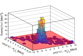
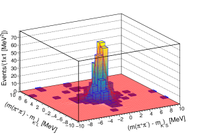
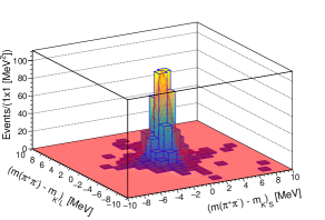
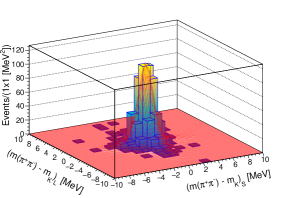
Figure 1: Invariant mass distribution of $\mathrm{K_{L}}$ vs $\mathrm{K_{S}}$ vertices for four $\Delta t$ bins: $0<\Delta t<1~{}\tau_{\rm S}$ (top left), $1<\Delta t<2~{}\tau_{\rm S}$ (top right), $2<\Delta t<3~{}\tau_{\rm S}$ (bottom left), and $3<\Delta t<4~{}\tau_{\rm S}$ (bottom right). The histograms of data have superimposed the result of the unbinned fit (red).

An unbinned maximum likelihood fit is performed in order to evaluate the number of background events. The model used to fit the observed distribution is:

$$N_{\rm obs}(x,y)=N_{S}\cdot S(x,y)+N_{B}\cdot G(z;\mu_{z}=0,\sigma_{B})~{},$$ (9)

with $x,y=\left[m(\pi^{+}\pi^{-})-m_{\mathrm{K}}\right]_{\rm S,L}$ the invariant mass shift for reconstructed $\mathrm{K_{S,L}}$ vertices, $S(x,y)$ the template for the signal shape obtained from MC after the selection, not imposing the invariant mass constraint, $G(z;\mu_{z}=0,\sigma_{B})$ a Gaussian distribution as a function of the variable $z=x+y$ with zero mean ($x=-y$) and standard deviation $\sigma_{B}$ (free parameter in the fit) to model the background along the second diagonal, $N_{S}$ and $N_{B}$ two normalization factors for signal and background, respectively. The background events are then extrapolated from the $|x,y|<10~{}\mathrm{MeV}$ region to the nominal signal region $|x,y|<5~{}\mathrm{MeV}$. The result is $n_{B,1}=39\pm 5$ events for the first bin ($0\leq\Delta t<1~{}\tau_{\rm S}$). The consistency of this result is checked against different extrapolating regions, from $|x,y|<6~{}\mathrm{MeV}$ to $|x,y|<10~{}\mathrm{MeV}$. The fit is independently repeated for the ($1<\Delta t<2~{}\tau_{\rm S}$), ($2<\Delta t<3~{}\tau_{\rm S}$), and ($3<\Delta t<4~{}\tau_{\rm S}$) bins yielding as result $n_{B,2}=6\pm 2$, $n_{B,3}=6\pm 2$, and $n_{B,4}=3\pm 1$ events, respectively. From these results we conclude that the $e^{+}e^{-}\rightarrow\pi^{+}\pi^{-}\pi^{+}\pi^{-}$ background can be considered negligible for $\Delta t>3~{}\tau_{\rm S}$.

The regeneration background peaks in the region at $\Delta t\approx 17~{}\tau_{\rm S}$ due to the spherical beam pipe kloeqm2006 . In the present analysis the fit to the $\Delta t$ distribution is restricted in the range $0<\Delta t<12~{}\tau_{\rm S}$ to avoid this background, while keeping the maximum sensitivity to the various decoherence and $\mathcal{CPT}$ violation parameters, which is mainly in the region $\Delta t<6~{}\tau_{\rm S}$. The remaining regeneration background is due to the small contribution from the thin beryllium cylinder, largely dominated by the incoherent over the coherent regeneration qmadd ; baldini . The latter can be therefore neglected. The $\Delta t$ distribution of the residual incoherent regeneration background is spread out over the region $5<\Delta t<12~{}\tau_{\rm S}$, as an effect of the cylindrical geometry, and is evaluated with Monte Carlo. The $\mathrm{K_{S}}$ regeneration probability, $P_{\rm reg}^{\rm cyl}$, is extrapolated from the measured regeneration probability on the spherical beam pipe kloeqm2006 , $P_{\rm reg}^{\rm sph}$, knowing the incoherent regeneration cross-section ratio for beryllium and aluminum, $r=\frac{\sigma_{\rm inc}(\rm Be)}{\sigma_{\rm inc}(\rm Al)}$, and using the relation:

$$P_{\rm reg}^{\rm cyl}=D_{\rm geom}\cdot P_{\rm reg}^{\rm sph}\cdot f(r)~{},$$ (10)

where $D_{\rm geom}$ is a factor depending on the beam pipe geometry, and $f(r)$ a function of the ratio $r$:

$$f(r)=\frac{(\rho_{\rm Be}/A_{\rm Be})\cdot r}{\rho_{\rm AlBe}\left(\frac{w_{\rm Be}}{A_{\rm Be}}\cdot r+\frac{w_{\rm Al}}{A_{\rm Al}}\right)}~{},$$ (11)

with $\rho_{\rm AlBe}$ the density of the spherical beam pipe, $w_{\rm Be}$ and $w_{\rm Al}$ the $\rm Be/Al$ proportion by weight. The large uncertainty on $r$ (from ref. baldini $r\approx 2$, while a preliminary KLOE measurement yields $r\approx 0.3$ iza ) reflects on $f(r)$, which is anyhow smoothly varying with $r$ reaching a plateau for $r\gtrsim 2$, and dominates the uncertainty on $P_{\rm reg}^{\rm cyl}$. This quantity is used as input to the MC evaluation of the true $\Delta t$ distribution with and without the effect of regeneration. The ratio between the two corresponding histograms provides the correction factors $R_{j}$ to account for regeneration background as a function of $\Delta t$ in the fit procedure described in section 6.

5 Efficiency evaluation

The total selection efficiency can be parametrized as the product:

$$\epsilon_{\rm tot}=\epsilon_{\rm trig}~{}\epsilon_{\rm reco}~{}\epsilon_{\rm cuts}~{},$$ (12)

with $\epsilon_{\rm trig}$ the efficiency due to the trigger, $\epsilon_{\rm reco}$ the efficiency of the reconstruction procedure and $\epsilon_{\rm cuts}$ the efficiency due to the selection cuts. The latter is derived from the MC, while the MC efficiencies of the first two are corrected using data from an independent control sample, as described in the following. It has to be underlined that for the present analysis only the dependence of $\epsilon_{t\rm ot}$ on $\Delta t$ is crucial, while its absolute global value is not relevant. The efficiency $\epsilon_{\rm tot}$ as obtained from MC is shown in figure 2 as a function of $\Delta t$, before and after the application of the kinematic fit and the cut on the opening angle. The efficiency is in average $\sim 25\%$ with a small reduction at $\Delta t\approx 0$ that is due to two concurrent effects: (i) longer extrapolation length for both tracks originating in the interaction point that enhances the probability to fail the reconstruction; (ii) the possible swap of tracks associated to two different kaon decay vertices, when the two vertices are close in time $\Delta t\approx 0$.

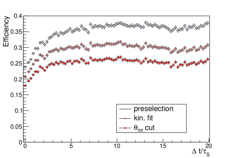
Figure 2: Efficiency evaluated from the Monte Carlo, after the preselection criteria applied (grey), the kinematic fit (brown), and the cut on the $\theta_{\pi\pi}$ angle (red). The vertical error bars indicate the statistical uncertainty of the Monte Carlo sample.

The trigger and reconstruction efficiencies provided by the MC are checked with data, using an independent control sample of $\mathrm{K_{S}}\mathrm{K_{L}}\rightarrow\pi^{+}\pi^{-}\pi\mu\nu$ events, selected to have high purity and to have an overlap with the momentum distribution of the signal. The applied selection criteria ensure the statistical independence of the control sample from the signal and a purity of $95\%$, with the residual background dominated by the $\mathrm{K_{S}}\mathrm{K_{L}}\rightarrow\pi^{+}\pi^{-}\pi e\nu$ decay. The efficiency correction has been evaluated as the ratio between data and MC $\Delta t$ distributions of $\mathrm{K_{S}}\mathrm{K_{L}}\rightarrow\pi^{+}\pi^{-}\pi\mu\nu$ events. A fit with a constant indicates a quite small average correction, as shown in figure 3.

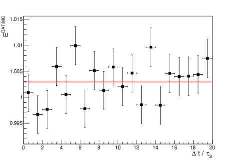
Figure 3: Data/MC efficiency correction as a function of $\Delta t$. The superimposed line is the result of a fit with a constant.

6 Fit

As already pointed out in section 4, the fit is performed on the measured $\Delta t$ distribution in the range $0<\Delta t<12~{}\tau_{\rm S}$, in order to minimize the regeneration background. The bin width of the data histogram is $\overline{\Delta t}=1~{}\tau_{\rm S}$, of the same size of the $\Delta t$ resolution. The fit function in the $j$-th true $\Delta t$ bin is evaluated integrating the decay intensities described in section 1 over the sum $(t_{1}+t_{2})$, at fixed $\Delta t$, and over the bin width:

$$I({\bf q})_{j}^{\rm th}=\int_{(j-1)\overline{\Delta t}}^{j\overline{\Delta t}}d(\Delta t)\int_{\Delta t}^{\infty}I(t_{1},t_{2}|{\bf q})~{}d(t_{1}+t_{2})~{},$$ (13)

with ${\bf q}$ the vector of the decoherence and $\mathcal{CPT}$ violation parameters. Then the following expression for the expected number of events in the $i$-th reconstructed $\Delta t$ bin is used to fit the observed $\Delta t$ distribution:

$$N({\bf q})_{i}^{\rm th}=\mathcal{N}E^{\frac{\rm DAT}{\rm MC}}_{i}\sum_{j}S_{i,j}\epsilon_{j}R_{j}I({\bf q})_{j}^{\rm th}$$ (14)

with $E_{i}^{\frac{\rm DAT}{\rm MC}}$ the data/MC efficiency correction discussed in section 5, $S_{i,j}$ the smearing matrix describing the $\Delta t$ resolution obtained from MC, $\epsilon_{j}$ the MC efficiency, $R_{j}$ a factor describing the regeneration contribution according to (10) and taking into account its $\Delta t$ shape, and $\mathcal{N}$ a global normalization factor. Finally the $4\pi$ background evaluated as described in section 4 is subtracted from the data histogram, with $N_{i}^{\rm data}$ the resulting number of observed events in the $i$-th bin. The following $\chi^{2}$ function is minimized by the fit:

$$\chi^{2}=\sum_{i}\left(\frac{N_{i}^{\rm data}-N({\bf q})_{i}^{\rm th}}{\sigma_{i}}\right)^{2}~{},$$ (15)

with $\sigma_{i}$ evaluated by summing in quadrature the statistical uncertainty of data and the subtracted $4\pi$ background, and including the uncertainties for MC efficiency and data/MC corrections. The measured $\Delta t$ distribution and, as an example, the result of the fit for the $\zeta_{\rm SL}$ decoherence model, are shown in figure 4; the total number of signal events from this fit is $10278\pm 105$.

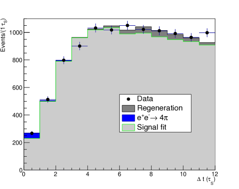
Figure 4: Data and fit distribution for the $\zeta_{\rm SL}$ decoherence model with background contributions displayed.

7 Systematic uncertainties

In order to evaluate the systematic uncertainty on the fit results, the whole fitting procedure is repeated varying the selection cuts, the number of background events, the $\Delta t$ resolution, and the physical constants given in input to the theoretical models, as described in the following.

• Selection Cut Stability – The selection cuts are all varied in order to test the MC in evaluating the corresponding efficiency variation. The cuts are varied according to their resolution $\sigma$ in steps of $\pm 1\sigma$ and $\pm 2\sigma$ to check the stability of the results. For the evaluation of the systematic uncertainty only the $\pm 1\sigma$ variation is considered. The uncertainties from the various cuts are added in quadrature, with the exception of the uncertainty due to the variation of the cut on the invariant mass of the two vertices, which is not considered. In fact the latter is strongly correlated with the variation of the $4\pi$ background contamination, which is the dominant effect in this case, and has to be correspondingly rescaled for each invariant mass cut (see section 4). Therefore the effect of the invariant mass cut variation is automatically included in the evaluation of the systematic uncertainty of the $4\pi$ background described below.

• $\mathbf{4\pi}$ Background – To vary the number of background events originated from the non-resonant pion production $e^{+}e^{-}\rightarrow\pi^{+}\pi^{-}\pi^{+}\pi^{-}$ process, the fit procedure is repeated rescaling the $n_{B,i}$ background yield according to the uncertainty of the total $4\pi$ background contribution $n_{B}=n_{B,1}+n_{B,2}+n_{B,3}=51.0\pm 5.7$.

• Regeneration – The factors $R_{j}$ describing the regeneration background as a function of $\Delta t$ are varied according to the $R^{\prime}_{j}=R_{j}+a\,(R_{j}-1)$ relation (no regeneration corresponds to $R_{j}=1$), where $a$ parametrizes the fractional variation due to the uncertainty on the regeneration process. The latter is dominated by the uncertainty on the knowledge of the cross-section ratio $r$ through the function $f(r)$, as discussed in section 4. A variation of $r$ in the range $\sim 0.3<r<\infty$ corresponds to a fractional variation in the range $-35\%<a<+10\%$, which is therefore considered for the evaluation of the systematic uncertainty due to regeneration.

• $\mathbf{\Delta t}$ Resolution – In order to evaluate the MC reliability on the $\Delta t$ resolution description, the proper decay time ($t_{\rm S}$) distribution of $\mathrm{K_{S}}\rightarrow\pi^{+}\pi^{-}$ events is obtained selecting a sample relaxing the boundary condition $\lambda_{\rm S}>0$ in the kinematic fit procedure, and requiring for the $\mathrm{K_{L}}$ a decay path of at least $12\mbox{~{}cm}$. This allows to compare the negative tail of the $t_{\rm S}$ distribution for data and MC, which corresponds to those events in which the $\mathrm{K_{S}}$ vertex is, because of resolution effects, between the $\phi$ and the $\mathrm{K_{L}}$ vertex. The $t_{\rm S}$ distribution is fit with an exponential function taking into account resolution effects by constructing a smearing matrix from MC. The accuracy of the MC description is evaluated by increasing or reducing the resolution by a scale factor $k$ according to the relation:

  $$\frac{\sigma^{\prime}_{\rm MC}}{\sigma_{\rm MC}}=k~{},$$ (16)

  where $\sigma_{\rm MC}=(t_{\rm S}^{\rm MC\,true}-t_{\rm S}^{\rm MC\,reco})$ and $\sigma_{\rm MC}^{\prime}=(t_{\rm S}^{\rm MC\,true}-t_{\rm S}^{\prime\,\rm MC\,reco})$, with $t_{\rm S}^{\rm MC\,reco}$ and $t_{\rm S}^{\rm MC\,true}$ the MC reconstructed and true $t_{\rm S}$, respectively. The new reconstructed time $t_{\rm S}^{\prime\,\rm MC\,reco}$ evaluated from equation (16) is then used to construct a modified smearing matrix. By fixing the normalization of the distribution to data and $\tau_{\rm S}$ to its known value kloelifetime , $\tau_{\rm S}=0.89562\times 10^{-10}\,\mathrm{s}$, a $\chi^{2}$ scan as a function of $k$ is performed to find the best value of the scale factor. The result is $k=0.9962\pm 0.0044$, which is compatible with unity with an uncertainty of 0.4%. As a cross-check, a fit with $\tau_{\rm S}$ as a free parameter (and $k=1$) yields as result $\tau_{\rm S}^{\mathrm{(fit)}}=(0.8952\pm 0.0030)\times 10^{-10}\,\mathrm{s}$.

  Similarly, the systematic uncertainty related to the $\Delta t$ resolution is evaluated by increasing or reducing the resolution and correspondingly modifying the smearing matrix $S_{i,j}$ using the relation:

  $$\frac{\Delta t^{\rm MC\,true}-\Delta t^{\prime\,\rm MC\,reco}}{\Delta t^{\rm MC\,true}-\Delta t^{\rm MC\,reco}}=1+\delta k~{},$$ (17)

  with $\Delta t^{\rm MC\,reco}$ and $\Delta t^{\rm MC\,true}$ the MC reconstructed and true $\Delta t$, respectively, and $\delta k=\pm 0.75\%,\pm 1.5\%$. The variation $\delta k=\pm 0.75\%$, larger by almost a factor two than the uncertainty on the scale factor $k$ discussed above, is considered for the evaluation of the systematic uncertainty.

• Input Physical Constants – In order to evaluate the effect induced by the uncertainty on the values of the physical constants ($\tau_{\rm S}$, $\tau_{\rm L}$, $\Delta m$, and $\eta_{+-}$) used in input to the fit theoretical function $I(t_{1},t_{2}|{\bf q})$, different sets of physical constants are randomly generated according to their uncertainty pdg , and the fit repeated for each set of constants. The standard deviation of the whole set of results is taken as systematic uncertainty.

The results on the various systematic uncertainty contributions are summarized in table 1. All contributions are evaluated, except for the one on the input physical constants, as the semi-distance between the maximum and minimum values among the results obtained with positive, negative, and no variation of the considered cut or effect. The final value of the systematic uncertainty is obtained by the sum in quadrature of the different contributions.

	$\delta\zeta_{\rm SL}$	$\delta\zeta_{0\bar{0}}$	$\delta\gamma$	$\delta\Re\omega$	$\delta\Im\omega$	$\delta|\omega|$	$\delta\phi_{\omega}$
	$\cdot 10^{2}$	$\cdot 10^{7}$	$\cdot 10^{21}$ GeV	$\cdot 10^{4}$	$\cdot 10^{4}$	$\cdot 10^{4}$	$({\rm rad})$
Cut stability	$0.56$	$2.9$	$0.33$	$0.53$	$0.65$	$0.78$	$0.07$
$4\pi$ background	$0.37$	$1.9$	$0.22$	$0.32$	$0.19$	$0.32$	$0.04$
Regeneration	$0.17$	$0.9$	$0.10$	$0.06$	$0.63$	$0.58$	$0.05$
$\Delta t$ resolution	$0.18$	$0.9$	$0.10$	$0.15$	$0.09$	$0.15$	$0.02$
Input phys. const.	$0.04$	$0.2$	$0.02$	$0.03$	$0.09$	$0.07$	$0.01$
Total	$0.71$	$3.7$	$0.42$	$0.64$	$0.93$	$1.04$	$0.10$

Table 1: Systematic uncertainties on all decoherence and $\mathcal{CPT}$-violating parameters.

8 Results

The final results for all models mentioned in section 1 are reported in the following.
For the decoherence parameters $\zeta_{\rm SL}$, $\zeta_{0\bar{0}}$, and $\gamma$ they are:

$$\zeta_{\rm SL}=(0.1\pm 1.6_{\rm stat}\pm 0.7_{\rm syst})\cdot 10^{-2}\hbox{~{}with~{}}\chi^{2}/{\hbox{dof}}=11.2/10~{},$$

$$\zeta_{0\bar{0}}=(-0.05\pm 0.80_{\rm stat}\pm 0.37_{\rm syst})\cdot 10^{-6}\hbox{~{}with~{}}\chi^{2}/{\hbox{dof}}=11.2/10~{},$$

$$\gamma=(0.13\pm 0.94_{\rm stat}\pm 0.42_{\rm syst})\cdot 10^{-21}\text{~{}GeV}\hbox{~{}with~{}}\chi^{2}/{\hbox{dof}}=11.2/10~{}.$$

The high precision of the $\zeta_{0\bar{0}}$ result with respect to $\zeta_{\rm SL}$ can be intuitively explained by considering that the overall decay, in which both kaons decay into $\pi^{+}\pi^{-}$, is suppressed by $\mathcal{CP}$ violation. In quantum mechanics this conclusion is independent on the basis used in the calculation of the decay intensity (2), while in case of a decoherence mechanism it depends on the basis into which the initial state tends to factorize. The decay $\mathrm{K_{S}}\mathrm{K_{L}}\rightarrow\pi^{+}\pi^{-}\pi^{+}\pi^{-}$ is still suppressed by $\mathcal{CP}$ violation, while the decay $\mathrm{K^{0}}\mathrm{\bar{K}^{0}}\propto(\mathrm{K_{L}}\mathrm{K_{S}}-\mathrm{K_{S}}\mathrm{K_{L}}+\mathrm{K_{S}}\mathrm{K_{S}}-\mathrm{K_{L}}\mathrm{K_{L}})\rightarrow\pi^{+}\pi^{-}\pi^{+}\pi^{-}$ has a contribution from $\mathrm{K_{S}}\mathrm{K_{S}}\rightarrow\pi^{+}\pi^{-}\pi^{+}\pi^{-}$ that it is not $\mathcal{CP}$ suppressed, and is copious in the region at $\Delta t\approx 0$. Consequently a larger sensitivity on the $\zeta_{0\bar{0}}$ parameter is achieved.

The $\lambda$ parameter derived from $\zeta_{\rm SL}$ bertlmann2 is:

$$\lambda=(0.1\pm 1.2_{\rm stat}\pm 0.5_{\rm syst})\cdot 10^{-16}\text{~{}GeV}~{}.$$

As these parameters are constrained to be positive, the results can be translated into $90\%$ confidence level (C.L.) upper limits feldman :

$$\zeta_{\rm SL}<0.030~{},$$

$$\zeta_{0\bar{0}}<1.4\cdot 10^{-6}~{},$$

$$\gamma<1.8\cdot 10^{-21}\text{ GeV }~{},$$

$$\lambda<2.2\cdot 10^{-16}\text{ GeV }~{}.$$

The results on the complex $\omega$ parameter have been obtained by performing the fit in Cartesian $\{\Re\omega,\Im\omega\}$ coordinates:

$$\Re\omega=(-2.3^{+1.9}_{-1.5{\rm stat}}\pm 0.6_{\rm syst})\cdot 10^{-4}~{},$$

$$\Im\omega=(-4.1^{+2.8}_{-2.6{\rm stat}}\pm 0.9_{\rm syst})\cdot 10^{-4}~{},$$

and in polar $\{|\omega|,\phi_{\omega}\}$ coordinates:

$$|\omega|=(4.7\pm 2.9_{\rm stat}\pm 1.0_{\rm syst})\cdot 10^{-4},$$

$$\phi_{\omega}=-2.1\pm 0.2_{\rm stat}\pm 0.1_{\rm syst}~{}\text{(rad)}~{}\hbox{~{}with~{}}\chi^{2}/{\hbox{dof}}=9.2/9~{}.$$

The correlation coefficient between $\Re\omega$ and $\Im\omega$ is 68%. The contour plot of $\Im\omega$ vs $\Re\omega$ for the $68\%$ and $95\%$ confidence levels is shown in figure 5.

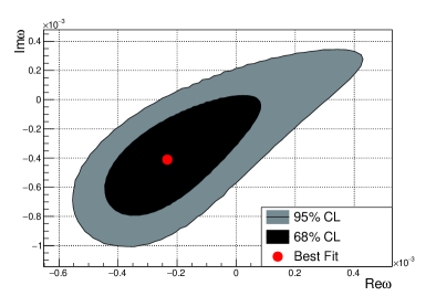
Figure 5: Contour plot of $\Im\omega$ vs $\Re\omega$ for $68\%$ and $95\%$ confidence levels.

The correlation coefficient between $|\omega|$ and $\phi_{\omega}$ is 14%. The contour plot of $|\omega|$ vs $\phi_{\omega}$ for the $68\%$ and $95\%$ confidence levels is shown in figure 6.

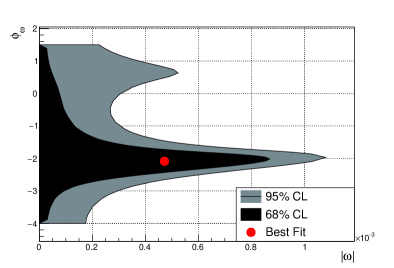
Figure 6: Contour plot of $\phi_{\omega}$ vs $|\omega|$ for $68\%$ and $95\%$ confidence levels.

These results represent a sizeable improvement with respect to previous measurements cplearzeta ; cplearabc ; bertlmann1 , in particular by more than a factor two with respect to previous KLOE results kloeqm2006 , and constitute the most stringent existing limits on the corresponding observable effects. All results are consistent with no decoherence and no $\mathcal{CPT}$ violation, while the precision in the cases of $\gamma$ and $\omega$ parameters is reaching, or surpassing, the level of the interesting Planck’s scale region, the scale at which, heuristically, these effects may appear in the most optimistic scenarios for quantum gravity ellis1 ; ellis2 ; ellisstring92 ; ellis2000 ; mavro1 ; mavro2 ; mavro3 .

Finally from the result on $|\omega|$, using relation (6) and the measured value of ${{\rm BR}(\phi\rightarrow\mathrm{K_{S}}\mathrm{K_{L}})}$ pdg , an upper limit for the branching ratio of the $\phi\rightarrow\mathrm{K_{S}}\mathrm{K_{S}},\mathrm{K_{L}}\mathrm{K_{L}}$ decay can be derived at 90% C.L.:

$${\rm BR}(\phi\rightarrow\mathrm{K_{S}}\mathrm{K_{S}},\mathrm{K_{L}}\mathrm{K_{L}})<2.4\cdot 10^{-7}~{}.$$

Appendix A Decay intensity expressions in decoherence models

$\zeta_{0\bar{0}}$ model

The decay intensity $I(t_{1},t_{2};\zeta_{0\bar{0}})$ is defined by introducing a factor $(1-\zeta_{0\bar{0}})$ multiplying the interference term of the quantum mechanical decay intensity expression in the $\{\mathrm{K^{0}},\mathrm{\bar{K}^{0}}\}$ basis:

$$I(t_{1},t_{2};\zeta_{0\bar{0}}) \propto \Big{|}\langle\pi^{+}\pi^{-}|T|\mathrm{K^{0}}(t_{1})\rangle\langle\pi^{+}\pi^{-}|T|\mathrm{\bar{K}^{0}}(t_{2})\rangle\Big{|}^{2}+\Big{|}\langle\pi^{+}\pi^{-}|T|\mathrm{\bar{K}^{0}}(t_{1})\rangle\langle\pi^{+}\pi^{-}|T|\mathrm{K^{0}}(t_{2})\rangle\Big{|}^{2}$$ (18)

$$-2(1-\zeta_{0\bar{0}})\,\Re\Big{[}\langle\pi^{+}\pi^{-}|T|\mathrm{K^{0}}(t_{1})\rangle\langle\pi^{+}\pi^{-}|T|\mathrm{\bar{K}^{0}}(t_{2})\rangle$$

$$\times\left(\langle\pi^{+}\pi^{-}|T|\mathrm{\bar{K}^{0}}(t_{1})\rangle\langle\pi^{+}\pi^{-}|T|\mathrm{K^{0}}(t_{2})\rangle\right)^{\ast}\Big{]}~{}.$$

The explicit expression for $I(t_{1},t_{2};\zeta_{0\bar{0}})$ to lowest order in $|\eta_{+-}|$ is:

$$I(t_{1},t_{2};\zeta_{0\bar{0}}) \propto \left[\left(1-\frac{\zeta_{0\bar{0}}}{2}\right)\left(e^{-\Gamma_{\rm L}t_{1}-\Gamma_{\rm S}t_{2}}+e^{-\Gamma_{\rm S}t_{1}-\Gamma_{\rm L}t_{2}}-2\,e^{-\frac{(\Gamma_{\rm S}+\Gamma_{\rm L})}{2}(t_{1}+t_{2})}\cos[\Delta m(t_{1}-t_{2})]\right)\right.$$ (19)

$$\left.+\frac{\zeta_{0\bar{0}}}{2}\left(\frac{e^{-\Gamma_{\rm S}(t_{1}+t_{2})}}{|\eta_{+-}|^{2}}-2\,e^{-\frac{(\Gamma_{\rm S}+\Gamma_{\rm L})}{2}(t_{1}+t_{2})}\cos[\Delta m(t_{1}+t_{2})]\right)\right]~{}.$$

$\lambda$ model

In the model described in ref. bertlmann2 decoherence is governed by a parameter $\lambda$ which is in direct correspondence to the parameter $\zeta_{\rm SL}$ introduced in eq.(3). The only difference in this case is that $\zeta_{\rm SL}$ becomes time dependent (see eq.(3.3) in Ref. bertlmann2 ):

$$\zeta_{\rm SL}(t_{1},t_{2})=1-e^{-\lambda\min(t_{1},t_{2})}~{}.$$ (20)

Substituting expression (20) in eq.(3) one obtains the decay intensity $I(t_{1},t_{2};\lambda)$:

$$I(t_{1},t_{2};\lambda) \propto e^{-\Gamma_{\rm L}t_{1}-\Gamma_{\rm S}t_{2}}+e^{-\Gamma_{\rm S}t_{1}-\Gamma_{\rm L}t_{2}}$$ (21)

$$-2\left(e^{-\lambda\min(t_{1},t_{2})}\right)e^{-\frac{(\Gamma_{\rm S}+\Gamma_{\rm L})}{2}(t_{1}+t_{2})}\cos[\Delta m(t_{1}-t_{2})]~{}.$$

As in our case the decoherence parameter $\zeta_{\rm SL}$ in eq.(3) is measured fitting the observed $\Delta t$ distribution, comparing the decay intensities (3) and (21) after integration on the sum $(t_{1}+t_{2})$, the following relationship holds:

$$\zeta_{\rm SL}=\frac{\lambda}{\Gamma_{\rm S}+\Gamma_{\rm L}+\lambda}\simeq\frac{\lambda}{\Gamma_{\rm S}}~{},$$ (22)

used to evaluate $\lambda$ from the measured $\zeta_{\rm SL}$ parameter.

$\gamma$ model

The explicit expression for $I(t_{1},t_{2};\gamma)$ is (see Ref. peskin ):

$$I(t_{1},t_{2};\gamma) \propto \left[\left(1+\frac{\gamma}{\Delta\Gamma|\eta_{+-}|^{2}}\right)\left(e^{-\Gamma_{\rm L}t_{1}-\Gamma_{\rm S}t_{2}}+e^{-\Gamma_{\rm S}t_{1}-\Gamma_{\rm L}t_{2}}\right)\right.$$ (23)

$$\left.-2\,e^{-\frac{(\Gamma_{\rm S}+\Gamma_{\rm L})}{2}(t_{1}+t_{2})}\cos[\Delta m(t_{1}-t_{2})]-2\frac{\gamma}{\Delta\Gamma|\eta_{+-}|^{2}}e^{-\Gamma_{\rm S}(t_{1}+t_{2})}\right]~{}.$$

$\omega$ model

The explicit expression for $I(t_{1},t_{2};\omega)$ is (see Ref. mavro2 ):

$$I(t_{1},t_{2};\omega) \propto \left[e^{-\Gamma_{\rm L}t_{1}-\Gamma_{\rm S}t_{2}}+e^{-\Gamma_{\rm S}t_{1}-\Gamma_{\rm L}t_{2}}-2\,e^{-\frac{(\Gamma_{\rm S}+\Gamma_{\rm L})}{2}(t_{1}+t_{2})}\cos[\Delta m(t_{1}-t_{2})]\right.$$ (24)

$$+\frac{|\omega|^{2}}{|\eta_{+-}|^{2}}e^{-\Gamma_{\rm S}(t_{1}+t_{2})}+2\frac{|\omega|}{|\eta_{+-}|}\left(e^{-\Gamma_{\rm S}t_{1}}e^{-\frac{(\Gamma_{\rm S}+\Gamma_{\rm L})}{2}t_{2}}\cos[\Delta m\,t_{2}-\phi_{+-}+\phi_{\omega}]\right.$$

$$\left.\left.-e^{-\Gamma_{\rm S}t_{2}}e^{-\frac{(\Gamma_{\rm S}+\Gamma_{\rm L})}{2}t_{1}}\cos[\Delta m\,t_{1}-\phi_{+-}+\phi_{\omega}]\right)\right]~{}.$$

- (1) A. Einstein, B. Podolsky, N. Rosen, Can quantum mechanical description of physical reality be considered complete?, Phys. Rev. 47 (1935) 777.
- (2) E. Schrödinger, Discussion of probability relations between separated systems, Math. Proc. Cambridge Phil. Soc. 31 (1935) 555
- (3) T. D. Lee, C. N. Yang, Reported by T. D. Lee at the Argonne National Laboratory, unpublished (1960), See text and footnotes in ref. day ; inglis .
- (4) T. B. Day, Demonstration of Quantum Mechanics in the large, Phys. Rev. 121 (1960) 1204.
- (5) D. R. Inglis, Completeness of Quantum Mechanics and Charge-Conjugation correlations of Theta particles, Rev. Mod. Phys. 33 (1961) 1.
- (6) H. J. Lipkin, CP violation and coherent decays of kaon pairs, Phys. Rev. 176 (1968) 1715.
- (7) I. Dunietz, J. Hauser, J. L. Rosner, Proposed experiment addressing CP and CPT violation in the - system, Phys. Rev. D 35 (1987) 2166.
- (8) C. D. Buchanan, R. Cousins, C. Dib, R. D. Peccei, J. Quackenbush, Testing CP and CPT violation in the neutral kaon system at a -factory, Phys. Rev. D 45 (1992) 4088.
- (9) G. D’Ambrosio, G. Isidori, A. Pugliese, CP and CPT measuremente at DANE, The second DANE handbook, Vol.I eds. L. Maiani, G. Pancheri, N. Paver, INFN-LNF, Frascati (1995) p.63.
- (10) A. Di Domenico (ed.), Handbook on Neutral Kaon Interferometry at a -factory, Frascati Phys. Ser. 43 INFN-LNF, Frascati, (2007); available online at http://www.lnf.infn.it/sis/frascatiseries/Volume43/volume43.pdf .
- (11) J. Bernabeu, A. Di Domenico, P. Villanueva-Perez, Direct test of time reversal symmetry in the entangled neutral kaon system at a -factory, Nucl. Phys. B 868 (2013) 102.
- (12) J. Bernabeu, A. Di Domenico, P. Villanueva-Perez, Probing CPT in transitions with entangled neutral kaons, JHEP 10 (2015) 139.
- (13) R. A. Bertlmann, W. Grimus, B. C. Hiesmayr, Quantum mechanics, Furry’s hypothesis, and a measure of decoherence in the system, Phys. Rev. D 60 (1999) 114032.
- (14) W. H. Furry, Note on the Quantum-Mechanical theory of measurement, Phys. Rev. 49 (1936) 393.
- (15) P. H. Eberhard, Tests of Quantum Mechanics at a -factory, The second DANE handbook, Vol.I eds. L. Maiani, G. Pancheri, N. Paver, INFN-LNF, Frascati (1995) p.99.
- (16) R. A. Bertlmann, K. Durstberger, B. C. Hiesmayr, Decoherence of entangled kaons and its connection to entanglement measures, Phys. Rev. A 68 (2003) 012111.
- (17) S. Hawking, The Unpredictability of Quantum Gravity, Commun. Math. Phys. 87 (1982) 395.
- (18) R. Wald, Quantum Gravity and Time reversibility, Phys. Rev. D 21 (1980) 2742.
- (19) J. Ellis, J. S. Hagelin, D. V. Nanopoulos, M. Srednicki, Search for violations of quantum mechanics, Nucl. Phys. B 241 (1984) 381.
- (20) J. Ellis, J. L. Lopez, N. .E. Mavromatos, D. V. Nanopoulos, Precision tests of CPT symmetry and quantum mechanics in the neutral kaon system, Phys. Rev. D 53 (1996) 3846.
- (21) J. Ellis, N. E. Mavromatos, D. V. Nanopoulos, String theory modifies quantum mechanics, Phys. Lett. B 292 (1992) 37.
- (22) J. Ellis, N. E. Mavromatos, D. V. Nanopoulos, How large are dissipative effects in noncritical Liouville string theory?, Phys. Rev. D 63 (2000) 024024.
- (23) P. Huet, M. E. Peskin, Violation of CPT and quantum mechanics in the system, Nucl. Phys. B 434 (1995) 3.
- (24) F. Benatti, F. Floreanini, Completely positive dynamical maps and the neutral kaon system, Nucl. Phys. B 488 (1997) 335.
- (25) J. Bernabeu, N. Mavromatos, J. Papavassiliou, Novel Type of CPT Violation for Correlated Einstein-Podolsky-Rosen States of Neutral Mesons, Phys. Rev. Lett. 92 (2004) 131601.
- (26) J. Bernabeu, N. E. Mavromatos, J. Papavassiliou, A. Waldron-Lauda, Intrinsic CPT violation and decoherence for entangled neutral mesons, Nucl. Phys. B 744 (2006) 180.
- (27) J. Bernabeu, N. E. Mavromatos, S. Sarkar, Decoherence induced CPT violation and entangled neutral mesons, Phys. Rev. D 74 (2006) 045014.
- (28) P. Zyla et al., (Particle Data Group), Review of Particle Physics, Prog. Theor. Exp. Phys. 2020 (2020) 083C01.
- (29) F. Ambrosino et al., Search for the decay with the KLOE experiment, Phys. Lett. B 679 (2009) 10.
- (30) F. Ambrosino et al., First observation of quantum interference in the process : a Test of quantum mechanics and CPT symmetry, Phys. Lett. B 642 (2006) 315.
- (31) D. Babusci et al., Test of CPT and Lorentz symmetry in entangled neutral kaons with the KLOE experiment, Phys. Lett. B 730 (2014) 89.
- (32) A. Gallo et al., DANE status report, Conf. Proc. C060626 (2006) 604.
- (33) M. Zobov et al., Test of crab-waist collisions at the DANE factory, Phys. Rev. Lett. 104 (2010) 174801.
- (34) C. Milardi et al., High luminosity interaction region design for collisions inside high field detector solenoid, JINST 7 (2012) T03002.
- (35) M. Adinolfi et al., The tracking detector of the KLOE experiment, Nucl. Instr. and Meth. A 488 (2002) 51.
- (36) M. Adinolfi et al., The KLOE electromagnetic calorimeter, Nucl. Instr. and Meth. A 482 (2002) 364.
- (37) M. Adinolfi et al., The trigger system of the KLOE experiment, Nucl. Instr. and Meth. A 492 (2002) 134.
- (38) F. Ambrosino et al., Data handling, reconstruction and simulation for the KLOE experiment Nucl. Instr. and Meth. A 534 (2004) 403.
- (39) A. Di Domenico, Testing quantum mechanics in the neutral kaon system at a -factory, Nucl. Phys. B 450 (1995) 293.
- (40) R. Baldini, A. Michetti, interactions and regeneration in KLOE, LNF-96-008 IR (1996) (available online at http://cds.cern.ch/record/316977/files/SCAN-9701034.pdf).
- (41) I. Balwierz, Measurement of the neutral kaon regeneration cross-section in beryllium at P=110 MeV/c with the KLOE detector, diploma thesis, Jagiellonian university, Krakow, (2011), (available online at http://koza.if.uj.edu.pl/staff/ibalwierz)
- (42) F. Ambrosino et al., Precision measurement of the meson lifetime with the KLOE detector, Eur. Phys. J. C 71 (2011) 1604.
- (43) G. J. Feldman, R. D. Cousins, Unified approach to the classical statistical analysis of small signals, Phys. Rev. D 57 (1998) 3873.
- (44) A. Apostolakis et al. An EPR experiment testing the nonseparability of the anti- wave function, Phys.Lett. B 422 (1998) 339.
- (45) R. Adler et al., Tests of CPT symmetry and quantum mechanics with experimental data from CPLEAR, Phys. Lett. B 364 (1995) 239.