When Cyber-Physical Systems Meet AI: A Benchmark, an Evaluation, and a Way Forward

Abstract.

Cyber-Physical Systems (CPS) have been broadly deployed in safety-critical domains, such as automotive systems, avionics, medical devices, etc. In recent years, Artificial Intelligence (AI) has been increasingly adopted to control CPS. Despite the popularity of AI-enabled CPS, few benchmarks are publicly available. There is also a lack of deep understanding on the performance and reliability of AI-enabled CPS across different industrial domains. To bridge this gap, we present a public benchmark of industry-level CPS in seven domains and build AI controllers for them via state-of-the-art deep reinforcement learning (DRL) methods. Based on that, we further perform a systematic evaluation of these AI-enabled systems with their traditional counterparts to identify current challenges and future opportunities. Our key findings include (1) AI controllers do not always outperform traditional controllers, (2) existing CPS testing techniques (falsification, specifically) fall short of analyzing AI-enabled CPS, and (3) building a hybrid system that strategically combines and switches between AI controllers and traditional controllers can achieve better performance across different domains. Our results highlight the need for new testing techniques for AI-enabled CPS and the need for more investigations into hybrid CPS to achieve optimal performance and reliability. Our benchmark, code, detailed evaluation results, and experiment scripts are available on https://sites.google.com/view/ai-cps-benchmark.

1. Introduction

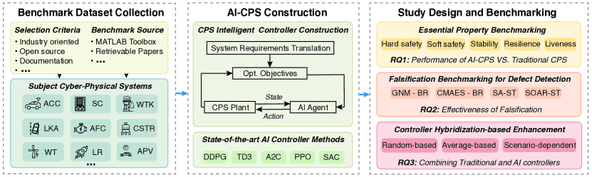
Figure 1. Workflow summary of AI-enabled CPS dataset and benchmark construction, and high-level empirical study design.

Cyber-Physical Systems (CPS) refer to the combination of mechanical and computer systems, in which computer systems actively monitor and control the behavior of mechanical systems according to system states and external environments. The integration of computer systems significantly improves the performance of mechanical systems. Nowadays, CPS have been widely deployed in diverse industrial domains, such as automotive systems, energy control, avionics, medical devices, etc.

With recent advances in Artificial Intelligence (AI), there has been increasing demand, from both industry and academia, in enhancing or even replacing traditional controllers with AI controllers (e.g., deep neural networks), in order to achieve more optimized and flexible control. Given the great learning and generalization capabilities of deep neural networks, AI controllers have been increasingly deployed in various domains to handle complex situations in the physical world (Liu et al., 2021; Nivison and Khargonekar, 2017).

Despite the rapid development of AI-enabled CPS, there is a lack of comprehensive analysis of their performance (e.g., safety, reliability, robustness) in different domains. The main reason is that unlike the large and growing open-source community in conventional software, CPS are often kept as private intellectual properties by industrial practitioners, in which strong domain knowledge and know-how are encoded. Therefore, even up to the present, very few benchmarks of AI-enabled CPS are publicly available for such analysis. Furthermore, since existing quality assurance methods such as falsification (Donzé, 2010; Annpureddy et al., 2011; Zhang et al., 2018; Dreossi et al., 2019; Yamagata et al., 2020; Adimoolam et al., 2017) are mostly designed for traditional CPS controllers, it is unclear to what extent these methods are still effective in analyzing AI controllers.

To bridge this gap, in this paper, we take the first step of benchmarking AI-enabled CPS in multiple industrial domains and performing a systematic analysis of their performance in comparison to their traditional counterparts. Fig. 1 shows our high-level study workflow. In particular, we investigate three main research questions to identify the challenges and potential opportunities for building safe and reliable AI-enabled CPS:

• RQ1. How well do the DRL-based AI controllers perform compared with the traditional controllers? This RQ aims to establish a comprehensive understanding of the advantages and limitations of both traditional and AI controllers in CPS. Our experiment shows that AI controllers do not always outperform their traditional counterparts. In several cases, AI controllers have weaknesses in handling multiple control outputs and fail to balance among multiple requirements.

• RQ2: To what extent are existing CPS testing methods still effective on AI-based CPS? Falsification is a commonly used technique to detect defects in traditional CPS. Although many falsification techniques have been proposed, it is still unclear whether they are still effective in the context of AI-enabled CPS. This RQ aims to establish a testing benchmark of different falsification methods on both traditional and AI-enabled CPS. Our comparative study finds that existing falsification methods are mostly designed for traditional controllers, and are not effective enough for AI-enabled CPS.

• RQ3: Can the combination of traditional and AI controllers bring better performance? In practice, building a hybrid controller that strategically switches between AI controllers and traditional controllers can be a promising direction for better performance (e.g., similar to component redundancies for safety in ISO 26262 (for Standardization, 2011)). This RQ aims to make an early investigation on whether this can be a promising direction in the context of AI-enabled CPS. Overall, we find that among the three types of hybrid controllers we explored, a scenario-dependent approach outperforms the other two in most of the cases. This result confirms that strategically combining traditional and AI controllers is a promising direction for further research.

In summary, this work makes the following contributions:

• We create the first public dataset and benchmark of AI-enabled CPS that span over various industrial domains, such as driving assistants, chemical reactor, aerospace, powertrains, etc. This provides a common ground for evaluating AI-based CPS and also enables further research along this direction.

• We perform a systematic analysis of the performance (e.g., safety, reliability, robustness) of AI-enabled CPS, and benchmarks the current techniques (e.g., falsification, system enhancement) as the basis for further investigation.

• Based on the analysis results, we further pose discussions on the future directions of AI-enabled CPS, including effectiveness of AI controllers, testing tools for AI-enabled CPS, and methods to construct hybrid control systems.

To the best of our knowledge, this is the very first paper that establishes a publicly available dataset and benchmark for industry-level CPS with AI controllers. The benchmark and our empirical study results demonstrate the potential research opportunities around AI-enabled CPS to meet the growing industrial demands. Our work enables better understanding, establishes the basis, and paves the path towards further quality assurance research to build safe and reliable AI-enabled CPS.

2. Background

This section gives an introduction on CPS and AI controllers for CPS. Specifically, we describe deep reinforcement learning (DRL) based AI controllers in this paper. We also briefly describe Signal Temporal Logic (STL), a specification language of CPS, and falsification, a typical and important testing method for CPS based on STL.

2.1. Cyber-Physical Systems and AI controllers

CPS have been widely adopted in safety-critical industrial domains, such as automotive systems, avionics, medical devices, etc. CPS make use of computer programs to monitor and control the behaviors of mechanical systems. Fig. 2(a) shows a brief overview of a CPS, which consists of a plant $M$ and a controller $C$. The plant is a physical environment, whose next state $y$ is decided by the current state and the control command $u$. The control command $u$ is issued by a software controller. Commonly-used traditional controllers include proportional integral derivative (PID) control, model predictive control (MPC), etc. (detailed in §3). These controllers make the control decision $u$ based on the state $y$ and an external input $i$.

In CPS, signals are passed between components in a system and between the system and the external environment. Formally, a signal $s\colon~{}[0,T]\to\mathbb{R}^{\mathsf{dim}}$ is defined as a time-variant function, where $T\in\mathbb{R}_{+}$ denotes the time horizon, and $\mathsf{dim}\in\mathbb{N}_{+}$ is called the dimension of the signal. In Fig. 2(a), the system state $y$, the control decision $u$, and the external input $i$ are all signals. Sensors and actuators are used to collect, process, and pass these signals between the plant $M$ and the controller $C$ in a CPS model.

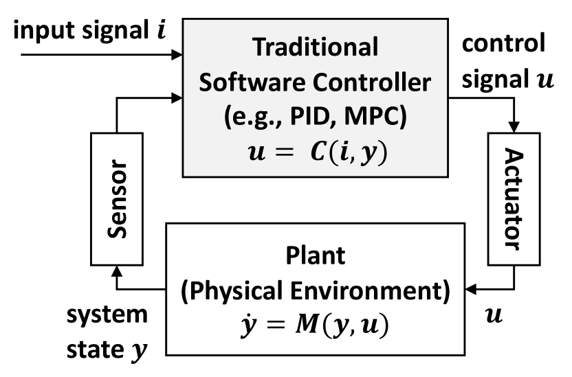
(a) Traditional CPS

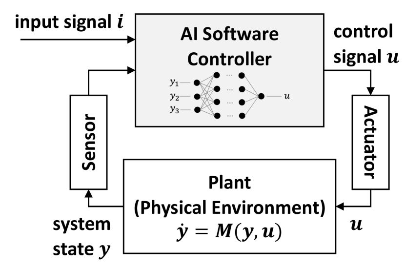
(b) AI-enabled CPS

Figure 2. Abstract workflow of CPS, with a traditional controller and an AI controller, respectively

AI Controller. With the boom of AI in the past few years, practitioners have started considering replacing traditional controllers with AI controllers. Fig. 2(b) gives an overview of AI-enabled CPS. An AI controller can be implemented and trained in different ways, such as supervised learning and reinforcement learning. Among different methods, deep reinforcement learning (DRL) is considered as the state-of-the-art, and has succeeded in various application domains (Arulkumaran et al., 2017). In this study, we mainly focus on DRL-based controllers. We briefly introduce DRL below.

Deep Reinforcement Learning. Unlike supervised learning, DRL does not require collecting labeled datasets beforehand. Instead, it follows the “trial-and-error” paradigm—learning the best strategy via repeated interactions with the external environment. Technically, DRL requires to train an agent in an environment so that the agent learns the best policy that maximizes the cumulative reward. At each step, the agent has a state given by the environment and the agent itself, and it is required to take an action to transit from the current state to a new one. A policy is a function that maps a state-action pair to a real-valued reward (Balakrishnan and Deshmukh, 2019). For a fixed state, the reward of each action depends on the feedback from the environment. In order to learn the best policy, the agent repeatedly tries an action to obtain a reward, and updates the policy accordingly. There is a variety of policy updating methods, such as Deep deterministic policy gradient (DDPG) (Lillicrap et al., 2015), Twin-delayed deep deterministic policy gradient (TD3) (Fujimoto et al., 2018), Actor-critic (A2C) (Donzé and Maler, 2010), Proximal policy optimization (PPO) (Schulman et al., 2017), Soft actor-critic (SAC) (Haarnoja et al., 2018), etc. We refer readers to (Johnson et al., 2020) for more details. DRL can be naturally applied to learn control policies for CPS by interacting with its plant, which is the physical environment of the system.

2.2. Temporal Specification of CPS

The behavior of a CPS is usually constrained by temporal requirements. Signal Temporal Logic (STL) is a widely adopted specification language to describe such requirements. In the following paragraphs, we briefly explain the syntax and semantics of STL.

STL Syntax. STL are composed of atomic propositions and formulas, defined as follows: $\alpha\,::\equiv\,f(x_{1},\dots,x_{N})>0,\;\varphi\,::\equiv\,\alpha\mid\bot\mid\neg\varphi\mid\varphi_{1}\wedge\varphi_{2}\mid\varphi_{1}\,\mathbin{\mathcal{U}_{I}}\varphi_{2}$ Here, $f$ is an $N$-ary function $f:\mathbb{R}^{N}\to\mathbb{R}$, $x_{1},\dots,x_{N}$ are variables, $I$ is a closed non-singular interval in $\mathbb{R}_{\geq 0}$, i.e., $I=[a,b]$ or $[a,\infty)$ where $a,b\in\mathbb{R}$ and $a<b$. $\mathbin{\mathcal{U}}$ denotes the until operator, and $\varphi_{1}\mathbin{\mathcal{U}_{I}}\varphi_{2}$ requires that $\varphi_{1}$ should be true during the interval $I$ until $\varphi_{2}$ becomes true. Other common connectives such as $\vee$, $\rightarrow,\top$, $\Box_{I}$ (always) and $\Diamond_{I}$ (eventually), are introduced as abbreviations: $\varphi_{1}\vee\varphi_{2}\equiv\neg\varphi_{1}\land\varphi_{2}$, $\varphi_{1}\rightarrow\varphi_{2}\equiv\neg\varphi_{1}\vee\varphi_{2}$, $\Diamond_{I}\varphi\equiv\top\mathbin{\mathcal{U}_{I}}\varphi$ and $\Box_{I}\varphi\equiv\lnot\Diamond_{I}\lnot\varphi$. An atomic formula $f(\vec{x})\leq c$, where $c\in\mathbb{R}$, is accommodated using $\lnot$ and the function $f^{\prime}(\vec{x}):=f(\vec{x})-c$.

Quantitative Robust Semantics. Traditional temporal logics (e.g., linear temporal logic) only have Boolean semantics that states the Boolean satisfaction of a formula. In contrast, STL is equipped with quantitative semantics (Donzé and Maler, 2010) that indicates not only if a formula is satisfied, but also how much a formula is satisfied.

Formally, the STL quantitative semantics ${\mathsf{Rob}(s,\varphi)}$ maps a signal $s$ and a STL formula $\varphi$ to a real number, which reflects how robustly $s$ satisfies $\varphi$. The larger this real number is, the further $s$ is from violating $\varphi$. If the number becomes negative, it indicates that $s$ violates $\varphi$. For example, let $s$ be a variable and $\varphi\equiv s>0$ be the specification. Then ${\mathsf{Rob}(s,\varphi)}$ can simply be the value of $s$: once $s$ is negative, $\varphi$ is violated. If interested, please refer to (Donzé and Maler, 2010) for the complete definition of STL robust semantics.

2.3. CPS Testing Methodology

Falsification is an established methodology in CPS testing (Annpureddy et al., 2011; Donzé, 2010; Zhang et al., 2018; Dreossi et al., 2019). Given a model $M^{C}$ and an STL specification $\varphi$, falsification searches for a counterexample input signal $i$ such that the corresponding output signal $M^{C}(i)$ violates $\varphi$. In this way, it proves the unsatisfiability of the system model $M^{C}$ to the specification $\varphi$.

Alg. 1 describes a basic falsification algorithm. Essentially, this algorithm formulates the testing problem as an optimization one, by taking the robustness as the objective function. In this algorithm, the CPS model $M^{C}$ is treated as a black box—only its input signal $i$ and the corresponding output signal $M^{C}(i)$ (system states) can be observed. In the main loop (Lines 5–9 in Alg. 1), falsification tries different input signals $i_{k}$ to minimize the robustness value $\mathsf{rb}_{k}$ computed based on $M^{C}(i_{k})$ and $\varphi$, so that the system is closer to violation of the specification $\varphi$. Once a negative robustness is observed, falsification will terminate and return that input as a counterexamples. Otherwise, it will keep searching until the time budget is run out (Line 10).

Algorithm 1 The classic falsification algorithm

1:CPS model $M^{C}$, an STL specification $\varphi$, a budget $B_{G}$.

2:function Hill-Climb-Falsify($M^{C},\varphi,B_{G}$)

3:    initialize a placeholder $i$ $\triangleright$ best input so far

4:    $\mathsf{rb}\leftarrow\infty$ $\triangleright$ minimum robustness so far

5:    for $k\in\{0,\ldots,B_{G}\}$ do

6:        $i_{k}\leftarrow\textsc{Hill-Climb}(\langle i_{l},\mathsf{rb}_{l}\rangle_{l=0,\ldots,k-1})$

7:        $\mathsf{rb}_{k}\leftarrow{\mathsf{Rob}(M^{C}(i_{k}),\varphi)}$ $\triangleright$ compute robustness

8:        if $\mathsf{rb}_{k}<\mathsf{rb}$ then

9:           $\mathsf{rb}\leftarrow\mathsf{rb}_{k}$, $i\leftarrow i_{k}$             

10:    return $\begin{cases}i&\text{if }\mathsf{rb}<0\\ \text{Failure}&\text{otherwise, no violation is found}\end{cases}$

To solve the optimization problem, falsification employs hill-climbing optimization algorithms, as shown in Line 6 of Alg. 1. Hill-climbing optimization algorithms are a family of stochastic meta-heuristics-based optimization algorithms. In general, these algorithms first do random sampling in the input space and obtain the robustness values of these inputs. Then based on the observations, they propose new samplings with the aim of decreasing robustness. Typical such algorithms include CMAES (Hansen et al., 2003), Global Nelder-Mead (Luersen and Le Riche, 2004), Simulated Annealing (Van Laarhoven and Aarts, 1987), etc.

3. Benchmark Collection

Table 1. The collected subject CPS

Subject CPS	Domain	Description	Type of Controller	#Blocks
Adaptive Cruise Control (ACC)	Driving assistant	Maintain a safety distance from a lead car	Model predictive control	297
Lane Keeping Assistant (LKA)	Driving assistant	Keep a vehicle in the center of a lane	Model predictive control	427
Automatic Parking Valet (APV)	Driving assistant	Park a vehicle on a target spot	Model predictive control	224
Exothermic Chemical Reactor (CSTR)	Chemical reactor	Promote a reactor transition of conversion rate	Model predictive control	316
Land a Rocket (LR)	Aerospace	Land a rocket on a target position	Model predictive control	175
Abstract Fuel Control (AFC)	Powertrain	Maintain the reference air-to-fuel ratio	PI & Feedforward control	281
Wind Turbine (WT)	Power grid	Maintain demanded values for key components	PID & Lookup table	161
Steam Condenser (SC)	Thermal systems	Maintain the reference pressure	PID control	56
Water Tank (WTK)	Water storage	Keep the water level at a reference value	PID control	919

3.1. Benchmark Collection

As most industrial CPS are treated as private intellectual properties and are kept confidential, it is challenging to find a large collection of practical and open-sourced CPS. We focus on two sources that potentially release open-sourced systems with documentations: (1) the distribution of Matlab control-related toolboxes, such as the model predictive control toolbox, and (2) CPS-related literature, such as the papers from software engineering and cyber-physical systems. Eventually, we selected nine industry-level CPS in seven domains based on the following criteria (see Table 1).

• Open-source. A CPS must be open-sourced so that we can modify the system to replace the traditional controller in it with AI controllers.

• Documentation. A CPS must have comprehensive documentation so that we can configure the system properly. Furthermore, to train AI controllers using DRL, we need to understand the system requirements to design proper reward functions in DRL.

• Complexity. A CPS must reflect the industrial complexity in order to get useful insights and implications from the experiments.

• Simulink. A CPS must use Simulink as its modeling platform. Simulink is a Matlab-based modeling environment developed by Mathworks and is widely adopted in industry. Having a consistent platform makes it easier to set up and run the benchmarks.

Table 1 gives an overview of the nine CPS in the benchmark. Specifically, Column #Blocks shows the number of blocks in each system, which is often used to measure the complexity of a CPS. Each system ships with a built-in traditional controller. We experiment with different types of learning algorithm, various agent configurations, and diverse reward functions to explore the capability of AI controllers. Among all variants, we select the best one as the final AI controller for each system. Due to the page limit, we elaborate on three representative systems (of different types) and their traditional controllers and AI controllers in the following section.

3.2. Three Representative CPS Examples

Adaptive Cruise Control (ACC). ACC is released by Mathworks (Mathworks, 2021). ACC is deployed in a driving environment with an ego car and a lead car. The goal of this system is to make the ego car move at a user-set velocity $v_{\mathit{set}}$ as long as the relative distance $d_{\mathit{rel}}$ between two cars is greater than the safety distance $d_{\mathit{safe}}$. The external input of the whole system is the acceleration of the lead car. The outputs include the velocity $v_{\mathit{ego}}$ and the position of the ego car.

The traditional controller used in this system is model predictive control (MPC). MPC achieves the optimal control at each moment by predicting the motions of the two cars in a finite time-horizon, and optimizing the acceleration of the ego car to maintain the safe distance. Specifically, MPC uses a linear model to predict the acceleration and velocity of both cars.

The DRL controller in ACC collects the system environment information to generate observation states. By evaluating the current state and computing a corresponding state value, the DRL controller outputs an acceleration command to the ego car. Unlike MPC, the DRL controller uses a reward function to evaluate the agent performance from two aspects: velocity and distance. While the safety distance $d_{\mathit{safe}}$ is secured, the ego car should approach to the cruise velocity $v_{\mathit{set}}$. Otherwise, it follows the lead car velocity to avoid collision. The reward function penalizes the agent by the violation of the safety distance requirement and rewards the agent based on how close the ego car velocity $v_{\mathit{ego}}$ is to the target speed.

Steam Condenser (SC). This system is collected from (Yaghoubi and Fainekos, 2019). As an indispensable part of modern steam power plants, SC is a sealed container where the steam is condensed by cooling water. The goal of the system is to maintain the pressure of condenser $P$ at a desired level $\mathit{P}_{\mathit{ref}}$. The external input of the system is the steam mass flow rate $\mathit{F}_{\mathit{s}}$ ($kg/s$). The output of the system is the internal pressure of the condenser. The traditional controller used in SC is a PID controller which outputs a cooling water flowrate. A typical PID controller includes three parameters: proportional (P), integral (I) and Derivative (D). $P$ reflects the current deviation of the system, $I$ mirrors the accumulations of past errors and $D$ represents on the anticipatory control. Through on-demand combination of the above three control parameters, the system error can be corrected.

The DRL controller in SC outputs a cooling water flowrate to maintain the condenser pressure at a desired level. It uses a reward function to make the condenser reach the desired pressure level as soon as possible and maintain this pressure until a new desired pressure is set. When the SC system moves to a steady state, the error signal may fluctuate at a small range. Then the reward function amplifies the error to improve the agent performance.

Abstract Fuel Control (AFC). AFC is a complex air-fuel control system released by Toyota (Jin et al., 2014). The whole system takes two input signals from the outside environment, $\mathit{PedalAngle}$ and $\mathit{EngineSpeed}$, and outputs $\mu=\frac{|\mathit{AF}-\mathit{AFref}|}{\mathit{AFref}}$, which is the deviation of the air-to-fuel ratio $\mathit{AF}$ from a reference value $\mathit{AFref}$. The goal of this system is to control the deviation $\mu$ no more than a predefined threshold.

The original control system consists of two parts: (1) a PI controller, and (2) a feed-forward controller. The former regulates the air-to-fuel ratio $\mathit{AF}$ in a closed loop, using the measured $\mathit{AF}$ to compute the fuel command. The latter estimates the rate of air flow into the cylinder by measuring of the inlet air mass flow rate.

The DRL controller in AFC gathers the information about engine dynamics and outputs a fuel command to achieve the reference $\mathit{AF}$ ratio. It uses a reward function to guide the agent to reduce the deviation $\mu$. Specifically, a positive reward is given based on how smaller $\mu$ is and a negative feedback is generated if $\mu$ exceeds certain threshold. A small penalty is added based on the DRL action value from the last time step to acquire a stable control output.

4. Study Design

As illustrated in Fig. 1, we perform experiments to answer three research questions. In RQ1, we evaluate the performance of AI-enabled CPS vs. traditional CPS. In RQ2, we evaluate the effectiveness of the existing falsification methods. In RQ3, we investigate the possibility of combining traditional and AI controllers. All experiments are based on system specifications from the official documentation (§4.1). These specifications further derive different metrics and experiment settings for each RQ, which we detail in §4.2.

4.1. System Specifications

Table 2. The STL specifications of the benchmark CPS. $\mathsf{S}1$ follows the pattern: $\Box_{I}(\varphi_{1})$; $\mathsf{S}2$ follows the pattern: $\Box_{I}(\varphi_{2})$; $\mathsf{S}3$ follows the pattern: $\Diamond_{I}\Box_{I^{\prime}}(\varphi_{3})$; $\mathsf{S}4$ follows the pattern: $\Box_{I}(\varphi_{41}\to\Diamond_{I^{\prime}}\varphi_{42})$; $\mathsf{S}5$ follows the pattern: $\Diamond_{I}(\varphi_{5})$;

Systems	$\mathsf{S}1$–hard safety	$\mathsf{S}2$–soft safety	$\mathsf{S}3$–steady state	$\mathsf{S}4$–resilience	$\mathsf{S}5$–liveness
ACC	$I=[0,50]$ $\varphi_{1}\equiv d_{\mathit{rel}}\geq d_{\mathit{safe}}$	$I=[0,50]$ $\varphi_{2}\equiv v_{\mathit{ego}}\leq v_{\mathit{set}}$	$I=[0,50],I^{\prime}=[0,40]$ $\varphi_{3}\equiv d_{\mathit{rel}}\geq d_{\mathit{safe}}+0.2$	$I=[0,50],I^{\prime}=[0,1]$ $\varphi_{41}\equiv\neg\varphi_{3},\varphi_{42}\equiv\varphi_{3}$	$I=[0,50]$ $\varphi_{5}\equiv v_{\mathit{ego}}\geq 1$
LKA	$I=[0,15]$ $\varphi_{1}\equiv|\mathit{error_{1}}|\leq 0.85$	$I=[0,15],\varphi_{2}\equiv\varphi_{21}\land\varphi_{22}$	$I=[0,15],I^{\prime}=[0,10]$ $\varphi_{3}\equiv|\mathit{error_{1}}|\leq 0.5$	$I=[0,15],I^{\prime}=[0,1]$ $\varphi_{41}\equiv\neg\varphi_{3},\varphi_{42}\equiv\varphi_{3}$	$I=[0,15]$ $\varphi_{5}\equiv|\mathit{v}|\geq 1$
		$\varphi_{22}\equiv|\mathit{error_{1}}|=0$
		$\varphi_{21}\equiv|\mathit{error_{2}}|=0$
APV	$I=[0,12]$ $\varphi_{1}\equiv|\mathit{error_{1}}|\leq 1$	$I=[0,12],\varphi_{2}\equiv\varphi_{21}\land\varphi_{22}$	$I=[0,12],I^{\prime}=[0,10]$ $\varphi_{3}\equiv|\mathit{error_{1}}|\leq 0.5$	$I=[0,12],I^{\prime}=[0,1]$ $\varphi_{41}\equiv\neg\varphi_{3},\varphi_{42}\equiv\varphi_{3}$	$I=[0,12]$ $\varphi_{5}\equiv|\mathit{v}|\geq 0.1$
		$\varphi_{21}\equiv|\mathit{error_{1}}|=0$
		$\varphi_{22}\equiv|\mathit{error_{2}}|=0$
CSTR	$I=[25,30]$ $\varphi_{1}\equiv|\mathit{error}|\leq 0.5$	$I=[25,30]$ $\varphi_{2}\equiv|\mathit{error}|=0$	$I=[25,30],I^{\prime}=[0,4]$ $\varphi_{3}\equiv|\mathit{error}|\leq 0.4$	—	—
LR	$I=[14.8,15]$ $\varphi_{1}\equiv|\mathit{error}|\leq 0.5$	$I=[14.8,15]$ $\varphi_{2}\equiv|\mathit{error}|=0$	—	—	$I=[0,15]$ $\varphi_{5}\equiv|\mathit{v}|\geq 0.1$
AFC	$I=[0,30]$ $\varphi_{1}\equiv\mu\leq 0.2$	$I=[0,30]$ $\varphi_{2}\equiv\mu=0$	$I=[0,30],I^{\prime}=[0,20]$ $\varphi_{3}\equiv\mu\leq 0.1$	$I=[0,30],I^{\prime}=[0,1]$ $\varphi_{41}\equiv\neg\varphi_{3},\varphi_{42}\equiv\varphi_{3}$	—
WT	$I=[30,630]$ $\varphi_{1}\equiv\theta\leq 14.2$	$I=[30,630]$ $\varphi_{2}\equiv\theta\ =0$	$I=[30,630],I^{\prime}=[0,500]$ $\varphi_{3}\equiv\theta\leq 14$	$I=[30,630],I^{\prime}=[0,5]$ $\varphi_{41}\equiv\neg\varphi_{3},\varphi_{42}\equiv\varphi_{3}$	—
SC	$I=[30,35]$ $\varphi_{1}\equiv|\mathit{error}|\leq 0.5$	$I=[30,35]$ $\varphi_{2}\equiv|\mathit{error}|=0$	$I=[30,35],I^{\prime}=[0,4]$ $\varphi_{3}\equiv|\mathit{error}|\leq 0.4$	—	—
WTK	$I=[5,6]\cup[11,12]\cup[17,18]$ $\varphi_{1}\equiv\ |\mathit{error}|\leq 0.2$	$I=[5,6]\cup[11,12]\cup[17,18]$ $\varphi_{2}\equiv\ |\mathit{error}|\ =0$	$I=[5,6]\cup[11,12]\cup[17,18]$	—	—
			$I^{\prime}=[0,0.8]$
			$\varphi_{3}\equiv|\mathit{error}|\leq 0.15$

In this work, we adopt STL (introduced in §2.2) as our specification language to evaluate the temporal properties of CPS. Specifically, we extract the temporal properties of the models from their documents, and summarize them in Table 2. We classify these properties into 5 categories, namely $\bm{\mathsf{S}}\mathbf{1}$-$\bm{\mathsf{S}}\mathbf{5}$, according to their semantics:

• $\bm{\mathsf{S}}\mathbf{1}$: Hard safety. $\mathsf{S}1$ must be strictly satisfied by the systems, any violation of $\mathsf{S}1$ can lead to safety problems. $\mathsf{S}1$ follows the pattern $\Box_{I}(\varphi_{1})$, where $\varphi_{1}$ is a system invariant during the simulation.

• $\bm{\mathsf{S}}\mathbf{2}$: Soft safety. $\mathsf{S}2$ follows the similar pattern $\Box_{I}(\varphi_{2})$ as $\mathsf{S}1$, but the satisfaction of $\varphi_{2}$ is not demanded. Instead, $\mathsf{S}2$ is used to measure the average and maximum deviations of the outputs from the reference values. Based on that, we can understand the average and boundary behaviors of the controllers.

• $\bm{\mathsf{S}}\mathbf{3}$: Steady state. $\mathsf{S}3$ follows the pattern $\Diamond_{I}\Box_{I^{\prime}}(\varphi_{3})$. It requires the system to satisfy $\varphi_{3}$ for the interval $I^{\prime}$ at some point in $I$. $\mathsf{S}3$ is used to evaluate if the system reaches the steady state $\varphi_{3}$ and stays there for the interval $I^{\prime}$.

• $\bm{\mathsf{S}}\mathbf{4}$: Resilience. $\mathsf{S}4$ follows the pattern $\Box_{I}(\varphi_{41}\to\Diamond_{I^{\prime}}\varphi_{42})$. It requires that, during the interval $I$, whenever an event $\varphi_{41}$ happens, the system should react by satisfying $\varphi_{42}$ within $I^{\prime}$. $\mathsf{S}4$ is used to evaluate the system’s ability to recover from fluctuations.

• $\bm{\mathsf{S}}\mathbf{5}$: Liveness. $\mathsf{S}5$ follows the pattern $\Diamond_{I}(\varphi_{5})$, where $\varphi_{5}$ should be eventually satisfied during $I$. $\mathsf{S}5$ is used to inspect the system to avoid the case when the controller makes conservative control decisions to passively meet the safety requirements.

4.2. Research Questions

RQ1. How well do the DRL-based AI controllers perform compared with the traditional controllers?

While many AI controllers have been proposed and used, there has not been a systematic study on how well AI controllers perform compared with traditional controllers. RQ1 aims to compare the performance of these two kinds of controllers and understand their pros and cons. Since DRL-based approaches are the state of the art among current AI controllers, we mainly focus on DRL-based controllers in this study. In the experiment, we first randomly generate 100 input signals. Then we run simulations on each of the CPS with the traditional controller and the DRL-based controller respectively. We compare the performances of these controllers according to multiple properties introduced in §4.1. To better understand the quality of the controllers, we not only consider Boolean satisfactions to the STL formulas in §4.1, but also propose a series of more fine-grained metrics that consider the semantics of different formula patterns. These fine-grained metrics for $\bm{\mathsf{S}}\mathbf{1}$-$\bm{\mathsf{S}}\mathbf{5}$ are listed as follows:

• $\bm{\mathsf{S}}\mathbf{1}$: We record the number of satisfying simulations $n_{s}$ and compute the satisfaction ratio over 100 rounds of simulation since $\mathsf{S}1$ are safety properties required to be satisfied strictly.

• $\bm{\mathsf{S}}\mathbf{2}$: In addition to the Boolean satisfaction of $\mathsf{S}2$, we are also interested in how much $\mathsf{S}2$ is violated in each case. Hence, given an output signal $s$, we first collect all the moments $T$ when $\varphi_{2}$ is violated. Then, we present two metrics regarding $\mathsf{S}2$: 1) MAE—the mean value of the average absolute error over 100 simulations, and 2) MAXERR—the mean value of the maximum absolute error over 100 simulations. With these two metrics, we can understand the average and the extreme violations, respectively.

• $\bm{\mathsf{S}}\mathbf{3}$: We use $\mathsf{S}3$ to extensively explore how stable the system is during each round of simulation. For 100 simulations, we record how many moments $T$ are there when $s(t)$ falls into a steady state defined by $\varphi_{3}$. Then we compute the percentage of these steady state moments by $\tfrac{\#T}{\#T_{\mathit{total}}}$ in each round of simulation. We take the average value over 100 simulations as the fine-grained metric to evaluate $\mathsf{S}3$.

• $\bm{\mathsf{S}}\mathbf{4}$: We use $\frac{\mathit{n_{r}}}{\mathit{n_{v}}}$ to measure how good the systems satisfy $\mathsf{S}4$ during one round of simulation, where $\mathit{n_{v}}$ is the number of cases when the system falls into the fluctuating state defined by $\varphi_{41}$, and $\mathit{n_{r}}$ is the number of the cases when the system can react by doing $\varphi_{42}$. We then take the average value of $\frac{\mathit{n_{r}}}{\mathit{n_{v}}}$ over 100 simulations.

• $\bm{\mathsf{S}}\mathbf{5}$: We record the number of simulation rounds $n_{s}$ satisfying $\mathsf{S}5$ in §4.1. Then we calculate the ratio of satisfaction over 100 rounds of simulation.

By analyzing the evaluation results with the metrics above, we can obtain more comprehensive information to understand the advantage and limitations of DRL-based AI controllers and traditional controllers, from multiple perspectives.

RQ2. To what extent are existing CPS testing methods still effective on AI-based CPS?

For RQ2, we focus on an established CPS testing methodology called falsification (introduced in § 2.3). Falsification has proved to be effective on traditional CPS (Yamagata et al., 2020; Zhang et al., 2018; Adimoolam et al., 2017), but few studies have evaluated it on AI controllers. Since falsification methods are guided by logic semantics, it is unclear whether it is still effective on AI controllers, which are essentially statistical methods with high uncertainty and low interpretability.

In the experiment, we select two widely-used falsification tools, Breach (Donzé, 2010) and S-TaLiRo(Annpureddy et al., 2011). Note that both Breach and S-TaLiRo integrate several different back-end optimization solvers, and apply different tricks to improve the performance. We select Global Nelder-Mead (GNM) and CMAES for Breach, and Simulated Annealing (SA) and stochastic optimization with adaptive restart (SOAR) (Mathesen et al., 2019) for S-TaLiRo according to the findings in (Ernst et al., 2020).

Due to the stochasticity of the falsification algorithms, for each experiment, we repeatedly run the falsification algorithms, and obtain a falsification rate $\frac{\text{\#~{}successful trials}}{\text{\#~{}total trials}}$ as the evaluation metric. We also report the average time consumption, and the average number of successful falsification trials as complementary metrics.

In this experiment, we only run falsification on the systems that never violate $\mathsf{S}1$ (hard safety) during random simulations in the experiment of RQ1. Because these systems are hard to be evaluated in RQ1, which can be used as the changeable samples to measure the performance difference among different falsification approaches.

Our results of RQ1 and RQ2 form a basic benchmark quality and reliability analysis of AI-enabled CPS.

RQ3. Can the combination of traditional and AI controllers bring better performance?

As suggested by international standards ISO26262 (for Standardization, 2011) and ISO/PAS 21448 (SOTIF) (for Standardization, 2019), modular redundancy (e.g., doubling or tripling) is an important way to improve system quality and reliability. Therefore, in RQ3, we aim to investigate the performance of hybrid controllers—a novel type of controllers which combines the traditional and DRL-based ones. We perform an exploration on three typical approaches for such combinations: (1) a random-based approach, (2) an average-based approach, and (3) a scenario-dependent approach, with the purpose to understand whether this could be a promising direction for further research.

• Random-based. This method chooses a signal randomly from two controllers and passes it to the subsequent components. Here, sample time is a hyperparameter that indicates how frequently the controller switches. We use 2 different sample times in our experiments: (1) 0.1 sec, which is the minimum system step time, and (2) 1 sec, which is a log scale increase for comparison.

• Average-based. This method takes the average value of the outputs of two controllers as the final output.

• Scenario-dependent. Based on the insights from the experiments of RQ1 and RQ2, we summarize the scenarios where different types of controllers perform well and design a dynamic controller switch logic to achieve the optimal control strategy. For instance, for a system with controller A and B, A may have smaller value on S2 (averaged error signal) while B may have better performance on S4 (resilience). A switch logic can be: if the error signal exceeds a specified threshold which indicates the system falls into an unsteady state, the control will be granted to B to quickly recover to the steady state, and A may take in charge to maintain a small error value under the steady state.

In RQ3, we use the same metrics from RQ1 and RQ2 to evaluate these hybrid controllers under the same experimental settings.

Hardware & Software Dependencies. DRL training is computationally intensive, so we use a server with 3.5GHz Intel i9-10920X CPU, 15GB RAM, and an NVIDIA TITAN V GPU. Other experiments (e.g., falsification) were conducted using Breach 1.9.0 with GNM and CMAES as solvers and S-TaLiRo 1.6.0 with SA and SOAR as solvers on an Amazon EC2 c4.xlarge server with 2.9GHz Intel Xeon E5-2666 CPU, 4 virtual CPU cores, and 8GB RAM.

5. Experimental Results

5.1. RQ1. Performance of AI-enabled CPS vs.  traditional CPS

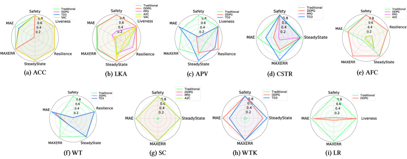
Figure 3. Performance comparison on systems with traditional and DRL controllers (RQ1)

Fig. 3 summarizes the evaluation results of traditional and AI-enabled CPS via radar charts. Each axis in a radar chart represents an evaluation metric from §4.1. We normalize the result of each metric into $[0,1]$. A higher value indicates a better performance.

• $\mathsf{S}1$: Hard safety. Not surprisingly, traditional controllers have better or at least comparable performance on $\mathsf{S}1$ in 7 of the 9 systems (ACC, LKA, APV, CSTR, LR, AFC, and WT), compared to DRL controllers. This is because safety always has the highest priority in the design of a traditional controller. However, in WTK and SC, the traditional PID controllers fail to regulate the error signals within a limited range. In particular, an oscillated signal can be generated by PID controllers and the maximum error threshold is therefore violated by an instantaneous overshoot.

  DRL controllers also have good performance on $\mathsf{S}1$ in 6 systems (ACC, LKA, CSTR, AFC, SC, and WTK). However, DRL controllers are better than traditional controllers in SC and WTK, while worse in WT and APV. Unlike the behavior of PID controllers in SC and WTK, DRL controllers output stable control signals with no instant overshoot. Thus, the safety requirements are held.

  Overall, for $\mathsf{S}1$, traditional controllers and DRL controllers have similar performance in systems like ACC, LKA, CSTR, and AFC. Also, for all systems, there is always at least one controller that never violates $\mathsf{S}1$. These results indicate that, the random sampling method cannot effectively evaluate systems on $\mathsf{S}1$, and therefore, we use the more advanced testing method, namely falsification, in RQ2 to acquire more in-depth insights.

• $\mathsf{S}2$: Soft safety. The traditional controllers have good MAE performance in 5 of the 9 systems (ACC, LKA, CSTR,LR, and AFC) and decent MAXERR performance in 5 systems (ACC, LKA, APV,LR, and WT). Compared with the results on $\mathsf{S}1$, there are fewer traditional CPS that outperform AI-enabled CPS on $\mathsf{S}2$. Moreover, a traditional controller with a good MAE result may not have a similarly good MAXERR result, e.g., AFC and CSTR. This indicates that the output signals from traditional controllers could be unstable, compared with DRL controllers.

  DRL controllers bring good MAE results in 7 systems (ACC, LKA, APV, WT, SC, LR, and WTK) and good MAXERR results in 6 systems (ACC, LKA, CSTR, AFC, SC, and WTK). According to these results, if a system has too many performance requirements or multiple control outputs, such as APV and WT, a standalone DRL controller may not handle these situations well.

• $\mathsf{S}3$: Steady state. Most traditional controllers can provide relatively stable outputs in all systems except SC and WTK. The poor performances of these two systems can be attributed to their oscillated PID outputs. In contrast, DRL controllers show good performance in all of the systems. Moreover, we find that different DRL controllers of the same system may have a variance in their performance. For instance, in WTK, while TD3 does not perform as well as DDPG in MAE, it outperforms DDPG in $\mathsf{S}3$.

• $\mathsf{S}4$: Resilience. Both DRL and traditional controllers show good performances regarding resilience in the 5 applicable systems, except the traditional and TD3 controllers in APV. This reveals their weaknesses in handling fluctuations. In contrast, although DDPG performs strongly in resilience, it does not conform to $\mathsf{S}1$, the hard safety requirements. For that reason, it can not be considered as a reliable system.

• $\mathsf{S}5$: Liveness. All the controllers show positive results on $\mathsf{S}5$. This indicates that none of our controllers takes conservative strategies to passively satisfy the safety requirements.

Regarding the comparison between the traditional controller and DRL controllers in each system, DRL controllers have better or similar performance in most of the systems. However, this is not always the case. For example, in APV and WT, the DRL-based controllers do not perform as well as their traditional counterparts.

Table 3. Falsification performance comparison between four existing falsification algorithms (RQ2)

	ACC-T			ACC-DDPG			ACC-TD3			ACC-SAC			CSTR-T			CSTR-DDPG			CSTR-PPO			CSTR-TD3
	FR	time	#sim	FR	time	#sim	FR	time	#sim	FR	time	#sim	FR	time	#sim	FR	time	#sim	FR	time	#sim	FR	time	#sim
GNM-BR	3	269.9	187.7	1	250.6	144.0	25	162.6	107.9	1	313.8	159.0	28	292.0	56.7	0	-	-	0	-	-	0	-	-
CMAES-BR	16	142.4	101.5	0	-	-	16	76.9	30.8	9	263.8	98.9	30	190.8	35.8	0	-	-	0	-	-	0	-	-
SA-ST	2	148.1	148.0	1	218.6	147.0	0	-	-	1	433.7	272.0	30	200.29	47.57	0	-	-	0	-	-	0	-	-
SOAR-ST	0	-	-	0	-	-	0	-	-	0	-	-	30	214.0	50.5	0	-	-	0	-	-	0	-	-

	AFC-T			AFC-DDPG			AFC-PPO			AFC-A2C			SC-T			SC-DDPG			SC-PPO			SC-A2C
	FR	time	#sim	FR	time	#sim	FR	time	#sim	FR	time	#sim	FR	time	#sim	FR	time	#sim	FR	time	#sim	FR	time	#sim
GNM-BR	0	-	-	0	-	-	30	9.5	6.8	30	9.4	6.1	30	0.3	1.0	0	-	-	0	-	-	0	-	-
CMAES-BR	0	-	-	0	-	-	10	37.1	28.9	4	77.3	61.3	30	0.3	1.0	0	-	-	0	-	-	0	-	-
SA-ST	9	295.2	148.4	0	-	-	0	-	-	0	-	-	30	0.2	1.0	0	-	-	0	-	-	0	-	-
SOAR-ST	11	411.3	157.4	0	-	-	0	-	-	0	-	-	30	0.2	1.0	0	-	-	0	-	-	0	-	-

	LKA-T			LKA-DDPG			LKA-PPO			LKA-A2C			LKA-SAC			APV-T			APV-DDPG			APV-TD3
	FR	time	#sim	FR	time	#sim	FR	time	#sim	FR	time	#sim	FR	time	#sim	FR	time	#sim	FR	time	#sim	FR	time	#sim
GNM-BR	30	636.9	75.4	0	-	-	30	10.6	10.9	30	5.0	5.0	30	60.5	54.0	0	-	-	30	41.5	1.0	30	42.8	1.0
CMAES-BR	27	414.9	47.8	0	-	-	28	21.6	16.6	30	9.4	7.5	28	82.3	44.4	0	-	-	30	51.6	1.0	30	59.7	1.0
SA-ST	24	1006.2	114.8	0	-	-	29	28.4	33.0	29	62.8	64.0	30	20.7	25.1	0	-	-	30	112.5	1.0	30	119.2	1.0
SOAR-ST	30	262.4	30.8	0	-	-	30	5.2	7.1	30	3.3	5.2	30	50.2	27.6	0	-	-	30	115.9	1.0	30	126.2	1.0

	WT-T			WT-DDPG			WT-PPO			WTK-T			WTK-DDPG			WTK-TD3			LR-T			LR-DDPG
	FR	time	#sim	FR	time	#sim	FR	time	#sim	FR	time	#sim	FR	time	#sim	FR	time	#sim	FR	time	#sim	FR	time	#sim
GNM-BR	30	197.8	42.9	0	-	-	0	-	-	30	3.3	5.8	0	-	-	0	-	-	20	4224.7	80.8	30	68.5	1.0
CMAES-BR	0	-	-	0	-	-	0	-	-	30	9.8	17.6	0	-	-	0	-	-	16	4341.1	78.4	30	54.9	1.0
SA-ST	20	335.5	65.4	0	-	-	0	-	-	30	8.8	20.6	0	-	-	0	-	-	13	6532.2	92.9	30	78.4	1.0
SOAR-ST	30	255.7	50.9	0	-	-	0	-	-	30	4.0	9.1	0	-	-	0	-	-	9	7809.1	93.2	30	83.7	1.0

5.2. RQ2. Effectiveness of Falsification

Table 3 shows the experimental results of RQ2, where we evaluate the performances of 4 falsification approaches using the metrics of FR (/30), time (secs), and #sim (see  §4.2). For each benchmark, we select their $\mathsf{S}1$, namely hard safety, as the target system specification. The reason is that, according to RQ1, we know that most of the systems do not violate their hard safety properties. Therefore, it makes sense to further investigate the satisfaction of each system to $\mathsf{S}1$. In our experiments, we set the budget ($B_{G}$ in Alg. 1) as 300. We highlight the best performer for each CPS model in Table 3, according to their FR.

The results presented in Table 3 reveal apparent differences in the abilities of different falsification algorithms for specific cases. For example, CMAES-BR performs well in ACC-T, but does not perform well in WT-T or AFC-A2C; SOAR-ST performs well in AFC-T, but does not perform well in ACC-TD3 or AFC-A2C.

We identify a model as falsifiable once there exists a falsification algorithm that manages to falsify the model. Based on our observations, we find that, for any falsification algorithm $\mathtt{A}$, there always exists a falsifiable benchmark that can not be falsified by $\mathtt{A}$. For instance, GNM-BR cannot falsify the falsifiable model AFC-T, and performs poorly on ACC-SAC; CMAES-BR cannot falsify the falsifiable model ACC-DDPG or WT-T; SA-ST cannot falsify the falsifiable model AFC-PPO or AFC-A2C; SOAR-ST cannot falsify the falsifiable model AFC-PPO or AFC-A2C. This result proves the famous no free lunch theorem in optimization (Wolpert and Macready, 1997), and also motivates us to develop more effective algorithms to handle these emerging AI-enabled CPS.

5.3. RQ3. Performance of Hybrid Controllers

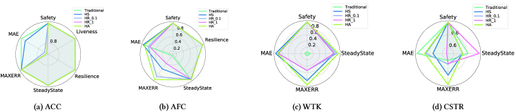
Figure 4. Performance comparison on systems with hybrid controllers (RQ3)

Table 4. Performance comparison on 4 hybrid benchmark CPS with falsification tools (RQ3)

Tool	GNM-BR			CMAES-BR			SA-ST			SOAR-ST
Benchmark	FR	time	#sim	FR	time	#sim	FR	time	#sim	FR	time	#sim
ACC-HS	0	-	-	11	177.9	71.5	2	465.4	188.0	0	-	-
ACC-HR_0.1	1	123.9	48.0	0	-	-	1	392.1	183.0	0	-	-
ACC-HR_1	3	313.1	121.0	1	66.2	26.0	1	457.6	209.0	0	-	-
ACC-HA	4	437.1	165.0	1	178.9	72.0	1	372.3	149.0	0	-	-
AFC-HS	0	-	-	0	-	-	0	-	-	0	-	-
AFC-HR_0.1	0	-	-	0	-	-	0	-	-	0	-	-
AFC-HR_1	29	148.5	87.4	30	105.1	61.0	0	-	-	0	-	-
AFC-HA	0	-	-	0	-	-	0	-	-	0	-	-
WTK-HS	0	-	-	0	-	-	0	-	-	0	-	-
WTK-HR_0.1	0	-	-	0	-	-	0	-	-	0	-	-
WTK-HR_1	0	-	-	0	-	-	0	-	-	0	-	-
WTK-HA	0	-	-	0	-	-	0	-	-	0	-	-
CSTR-HS	3	835.8	155.0	1	1310.6	292.0	10	997.7	213.4	11	973.5	172.1
CSTR-HR_0.1	0	-	-	0	-	-	0	-	-	0	-	-
CSTR-HR_1	22	411.2	87.6	20	155.8	33.2	18	578.7	124.0	30	369.0	61.9
CSTR-HA	0	-	-	0	-	-	0	-	-	1	1940.4	189.0

From the results of RQ1 and RQ2, we find that traditional and AI controllers have their own advantages in satisfying different requirements. For example, in CSTR (Fig. 3d), although the traditional controller performs well in MAE, it does not perform well in MAXERR. In contrast, the TD3 controller complements the situation, holding a high MAXERR but low MAE. This inspires us to combine traditional and AI controllers to obtain hybrid controllers, which may outperform each of them alone. We explore three combination methods, namely the random-based, the average-based, and the scenario-dependent ones, introduced in §4.2. For the random-based methods, we evaluate on multiple instances varied by their sampling time. Our results include Fig. 4 that uses the same evaluation metrics as RQ1, and Table 4 that applies the 4 falsification methods to those hybrid controllers.

• ACC. From the Fig. 4 and Table 4, in ACC, all the hybrid controllers perform better in falsification than the traditional controllers, and the scenario-dependent hybrid controller performs well in MAE compared to the traditional controller. In contrast, the performances of the random-based or the average-based hybrid controllers are not as good as the scenario-dependent ones.

• AFC. Among the 4 types of hybrid controllers we deployed, 3 of them have similar or better performance than the traditional one.

• WTK. The scenario-dependent and the average-based hybrid controllers are significantly better than the random-based controllers, and none of the hybrid controllers have been falsified.

• CSTR. We find that, the random-based method controller HR_0.1 and the average-based controller are not falsified. Moreover, the average-based controller also performs well in MAXERR as its constituent TD3 controller does.

In summary, the hybrid controllers can take advantage of their constituent controllers. The results reflect that the random-based combination method with large sample time can lead to an inconsistent control logic, and it can cause serious safety issues. The average-based method can be applied if the system is too complicated to design a controller switching logic and/or the constituent controllers have distinct advantages in different aspects. The scenario-dependent approach is recommended as it can switch between different controllers based on real-time system states. Moreover, the controller switching logic should be exclusively designed to fit the characteristics of the candidate controllers.

6. Discussions, Future Directions and Threats to Validity

Discussions. According to our insights from RQ1, DRL controllers may fall short of handling multiple control outputs or balancing multiple requirements simultaneously, compared to their traditional counterparts. Indeed, the design of reward function may be too complicated to compensate the balance among different requirements, since rewarding only a portion of the requirements may overshadow others. In industry, it is a common scenario to handle multiple requirements simultaneously. Therefore, applying DRL-based AI controllers in these cases requires further research.

Based on our evaluation of existing falsification algorithms, we find that falsification may not work effectively for AI-enabled CPS. AI controllers have their specific structure and unique decision logic, which is quite different from their traditional counterparts. Therefore, taking into account the characteristics of this specific formalism is important for effective testing.

The combination of different types of controllers offers a new direction of improving the safety and performance of the controllers, as demonstrated by our evaluation. Specifically, the scenario-dependent approach outperforms others, showing that strategic combination is necessary to achieve superior performances.

Future Directions. Based on the insights from our evaluation, we propose the following three future directions for AI-enabled CPS.

• First, there is a need for more research efforts on benchmarks and empirical studies in this direction. Moreover, more complicated system requirements that reflect industrial standards or demands should also be considered for further evaluation;

• Second, according to RQ2, existing falsification tools are not fully effective in detecting requirement violations in AI-based CPS. This offers a research opportunity of developing more advanced testing techniques for AI-enabled CPS, e.g., by exploiting the specific structure of neural networks for more effective testing;

• Third, besides testing, analysis techniques should be developed to understand the root cause of the violations. To achieve this, more research efforts on fault localization and repair are necessary.

Threats to Validity. In terms of construct validity, one potential threat is that the evaluation metrics may not fully describe the performance of controllers. To mitigate this threat, we used five evaluation metrics and two falsification tools to comprehensively measure and analyze the performance and reliability of CPS in our benchmark. In terms of internal validity, one potential threat is that the behavior of a CPS can vary when using different environment parameters. To mitigate this threat, we chose to use the same parameters as described in the documentation of each CPS to keep consistency. Further, we confirmed that our simulation results are consistent with the source descriptions and demos. In terms of external validity, one potential threat is that our analysis results may not be generalized to other CPS. To mitigate this threat, we tried our best to collect a diverse set of CPS with different functionalities, system environments, and control tasks.

7. Related Work

CPS Benchmarks. As mentioned in §3, collecting benchmarks of CPS is challenging. An annual workshop, namely ARCH, aims to mitigate this problem by bringing together CPS benchmarks and holding competitions for different research topics. The most relevant competitions to this paper are Artificial Intelligence and Neural Network Control Systems (Johnson et al., 2020) and Falsification (Ernst et al., 2020). However, the benchmark in (Ernst et al., 2020) only includes traditional CPS rather than AI-enabled CPS. While the benchmark in (Johnson et al., 2020) includes AI-enabled CPS, their benchmark includes less and simpler CPS such as Cart-Pole, which are not from industrial application domains.

AI Controllers for CPS. Duan et al. (Duan et al., 2016) proposed a benchmark on continuous control tasks. However, this benchmark involves game scenarios only such as Cart-Pole and Inverted Pendulum, rather than complex real-world environments. Besides DRL, FNN also has been used in designing a tracking controller for a robot manipulator (Braganza et al., 2007); however, the FNN controller is a subsystem which can only be used to compensate a feedback controller.

CPS Testing and Verification. Currently, most of the research efforts are devoted to formal verification of such systems, since it can give rigorous proofs on their safety. For example, reachability analysis (Tran et al., 2019; Xiang et al., 2018; Huang et al., 2019) has been extensively studied and considered as one of the most effective ways to verify AI controllers. The other line of formal verification of AI controllers is based on constraint solving, such as DLV (Huang et al., 2017), etc. Due to the intrinsic scalability problem of verification, their evaluations are usually on simple benchmarks. Falsification is considered as a method that suffers much less from the scalability issue than verification, and this is confirmed by the empirical study (Nejati et al., 2019), in which they compared the effectiveness of model checking and testing on CPS. However, existing falsification research mostly focuses on CPS with traditional controllers, and does not consider the specific structure of neural networks.

8. Conclusion

This paper presents a public benchmark of AI-enabled CPS in various domains, which can serve as a fundamental evaluation and testing framework for enhancing the understanding and development of AI-enabled CPS. Based on this benchmark, we collected a series of evaluation metrics and measured the performance and reliability of state-of-the-art deep reinforcement learning (DRL) controllers on various types of CPS. Our findings reveal some strengths and weaknesses of AI-enabled CPS and highlights an opportunity of strategically combining AI-enabled CPS with traditional CPS. Furthermore, our analysis of two widely used falsification techniques on AI-enabled CPS motivates further improvement of these techniques to account for the unique characteristics of AI controllers, in order to build safe and reliable CPS in the age of AI.

References

- (1)
- Adimoolam et al. (2017) Arvind Adimoolam, Thao Dang, Alexandre Donzé, James Kapinski, and Xiaoqing Jin. 2017. Classification and coverage-based falsification for embedded control systems. In CAV. Springer, 483–503.
- Annpureddy et al. (2011) Yashwanth Annpureddy, Che Liu, Georgios Fainekos, and Sriram Sankaranarayanan. 2011. S-taliro: A tool for temporal logic falsification for hybrid systems. In TACAS. Springer, 254–257.
- Arulkumaran et al. (2017) Kai Arulkumaran, Marc Peter Deisenroth, Miles Brundage, and Anil Anthony Bharath. 2017. Deep reinforcement learning: A brief survey. IEEE Signal Processing Magazine 34, 6 (2017), 26–38.
- Balakrishnan and Deshmukh (2019) Anand Balakrishnan and Jyotirmoy V Deshmukh. 2019. Structured reward shaping using signal temporal logic specifications. In 2019 IEEE/RSJ International Conference on Intelligent Robots and Systems (IROS). IEEE, 3481–3486.
- Braganza et al. (2007) David Braganza, Darren M Dawson, Ian D Walker, and Nitendra Nath. 2007. A neural network controller for continuum robots. TR 23, 6 (2007), 1270–1277.
- Donzé (2010) Alexandre Donzé. 2010. Breach, a toolbox for verification and parameter synthesis of hybrid systems. In CAV. Springer, 167–170.
- Donzé and Maler (2010) Alexandre Donzé and Oded Maler. 2010. Robust satisfaction of temporal logic over real-valued signals. In FORMATS. Springer, 92–106.
- Dreossi et al. (2019) Tommaso Dreossi, Alexandre Donzé, and Sanjit A Seshia. 2019. Compositional falsification of cyber-physical systems with machine learning components. JAR 63, 4 (2019), 1031–1053.
- Duan et al. (2016) Yan Duan, Xi Chen, Rein Houthooft, John Schulman, and Pieter Abbeel. 2016. Benchmarking deep reinforcement learning for continuous control. In ICML. PMLR, 1329–1338.
- Ernst et al. (2020) Gidon Ernst, Paolo Arcaini, Ismail Bennani, Alexandre Donze, Georgios Fainekos, et al. 2020. Arch-comp 2020 category report: Falsification. EPiC Series in Computing (2020).
- for Standardization (2011) International Organization for Standardization. 2011. ISO 26262:Road vehicles - Functional safety.
- for Standardization (2019) International Organization for Standardization. 2019. ISO/PAS 21448: Road vehicles - Safety of the intended functionality.
- Fujimoto et al. (2018) Scott Fujimoto, Herke Hoof, and David Meger. 2018. Addressing function approximation error in actor-critic methods. In ICML. PMLR, 1587–1596.
- Haarnoja et al. (2018) Tuomas Haarnoja, Aurick Zhou, Pieter Abbeel, and Sergey Levine. 2018. Soft Actor-Critic: Off-Policy Maximum Entropy Deep Reinforcement Learning with a Stochastic Actor. In ICML. 1861–1870.
- Hansen et al. (2003) Nikolaus Hansen, Sibylle D Müller, and Petros Koumoutsakos. 2003. Reducing the time complexity of the derandomized evolution strategy with covariance matrix adaptation (CMA-ES). Evolutionary computation 11, 1 (2003), 1–18.
- Huang et al. (2019) Chao Huang, Jiameng Fan, Wenchao Li, Xin Chen, and Qi Zhu. 2019. Reachnn: Reachability analysis of neural-network controlled systems. TECS 18, 5s (2019), 1–22.
- Huang et al. (2017) Xiaowei Huang, Marta Kwiatkowska, Sen Wang, and Min Wu. 2017. Safety verification of deep neural networks. In CAV. Springer, 3–29.
- Jin et al. (2014) Xiaoqing Jin, Jyotirmoy V Deshmukh, James Kapinski, Koichi Ueda, and Ken Butts. 2014. Powertrain control verification benchmark. In HSCC. 253–262.
- Johnson et al. (2020) Taylor T Johnson, Diego Manzanas Lopez, Patrick Musau, Hoang-Dung Tran, Elena Botoeva, Francesco Leofante, Amir Maleki, Chelsea Sidrane, Jiameng Fan, and Chao Huang. 2020. ARCH-COMP20 Category Report: Artificial Intelligence and Neural Network Control Systems (AINNCS) for Continuous and Hybrid Systems Plants. EPiC Series in Computing 74 (2020).
- Lillicrap et al. (2015) Timothy P Lillicrap, Jonathan J Hunt, Alexander Pritzel, Nicolas Heess, Tom Erez, Yuval Tassa, David Silver, and Daan Wierstra. 2015. Continuous control with deep reinforcement learning. arXiv preprint arXiv:1509.02971 (2015).
- Liu et al. (2021) Wenliang Liu, Noushin Mehdipour, and Calin Belta. 2021. Recurrent neural network controllers for signal temporal logic specifications subject to safety constraints. IEEE Control Systems Letters (2021).
- Luersen and Le Riche (2004) Marco A Luersen and Rodolphe Le Riche. 2004. Globalized Nelder–Mead method for engineering optimization. Computers & structures 82, 23-26 (2004), 2251–2260.
- Mathesen et al. (2019) Logan Mathesen, Shakiba Yaghoubi, Giulia Pedrielli, and Georgios Fainekos. 2019. Falsification of cyber-physical systems with robustness uncertainty quantification through stochastic optimization with adaptive restart. In CASE. IEEE, 991–997.
- Mathworks (2021) Mathworks. 2021. Adaptive Cruise Control System Using Model Predictive Control. https://www.mathworks.com/help/mpc/ug/adaptive-cruise-control-using-model-predictive-controller.html
- Nejati et al. (2019) Shiva Nejati, Khouloud Gaaloul, Claudio Menghi, Lionel C Briand, Stephen Foster, and David Wolfe. 2019. Evaluating model testing and model checking for finding requirements violations in Simulink models. In ESEC/FSE. 1015–1025.
- Nivison and Khargonekar (2017) Scott A Nivison and Pramod P Khargonekar. 2017. Development of a robust deep recurrent neural network controller for flight applications. In ACC. IEEE, 5336–5342.
- Schulman et al. (2017) John Schulman, Filip Wolski, Prafulla Dhariwal, Alec Radford, and Oleg Klimov. 2017. Proximal policy optimization algorithms. arXiv preprint arXiv:1707.06347 (2017).
- Tran et al. (2019) Hoang-Dung Tran, Diago Manzanas Lopez, Patrick Musau, Xiaodong Yang, Luan Viet Nguyen, Weiming Xiang, and Taylor T Johnson. 2019. Star-based reachability analysis of deep neural networks. In FM. Springer, 670–686.
- Van Laarhoven and Aarts (1987) Peter JM Van Laarhoven and Emile HL Aarts. 1987. Simulated annealing. In Simulated annealing: Theory and applications. Springer, 7–15.
- Wolpert and Macready (1997) David H Wolpert and William G Macready. 1997. No free lunch theorems for optimization. TEC 1, 1 (1997), 67–82.
- Xiang et al. (2018) Weiming Xiang, Hoang-Dung Tran, and Taylor T Johnson. 2018. Output reachable set estimation and verification for multilayer neural networks. TNNLS 29, 11 (2018), 5777–5783.
- Yaghoubi and Fainekos (2019) Shakiba Yaghoubi and Georgios Fainekos. 2019. Gray-box adversarial testing for control systems with machine learning components. In HSCC. 179–184.
- Yamagata et al. (2020) Yoriyuki Yamagata, Shuang Liu, Takumi Akazaki, Yihai Duan, and Jianye Hao. 2020. Falsification of cyber-physical systems using deep reinforcement learning. TSE (2020).
- Zhang et al. (2018) Zhenya Zhang, Gidon Ernst, Sean Sedwards, Paolo Arcaini, and Ichiro Hasuo. 2018. Two-layered falsification of hybrid systems guided by monte carlo tree search. TCAD 37, 11 (2018), 2894–2905.