Variations of Renormalized Volume for Minimal Submanifolds of Poincare-Einstein Manifolds

Abstract

We investigate the asymptotic expansion and the renormalized volume of minimal submanifolds, $Y^{m}$ of arbitrary codimension in Poincare-Einstein manifolds, $M^{n+1}$. In particular, we derive formulae for the first and second variations of renormalized volume for $Y^{m}\subseteq M^{n+1}$ when $m<n+1$. We apply our formulae to the codimension $1$ and the $M=\mathbb{H}^{n+1}$ case, exhibiting a small correction to [2] when $n=2$. Furthermore, we prove the existence of an asymptotic description of our minimal submanifold, $Y$, over the boundary cylinder $\partial Y\times\mathbb{R}^{+}$, and we further derive an $L^{2}$-inner-product relationship between $u_{2}$ and $u_{m+1}$ when $M=\mathbb{H}^{n+1}$. Our results apply to a slightly more general class of manifolds, which are conformally compact with a metric that has an even expansion up to high order near the boundary.

1 Introduction

We consider the half-space model of $\mathbb{H}^{n+1}=\{(y,x)\;|\;y\in\mathbb{R}^{n},\;\;x\in\mathbb{R}^{+}\}$ equipped with the complete metric

$$g=\frac{dy_{1}^{2}+\dots+dy_{n}^{2}+dx^{2}}{x^{2}}$$

Renormalized volume arises by trying to make sense of the $m$-dimensional volume of noncompact $Y^{m}\subseteq\mathbb{H}^{n+1}$ which intersect $\partial\mathbb{H}^{n+1}$ in a compact $(m-1)$-submanifold, $\gamma$, $C^{m+1,\alpha}$-embedded in $\partial\mathbb{H}^{n+1}=\mathbb{R}^{n}$. The hyperbolic metric is singular along the boundary $\partial\mathbb{H}^{n+1}=\{x=0\}$, and the $m$-dimensional volume is a priori infinite. But because $\partial Y=\gamma\subseteq\mathbb{R}^{n}$ is prescribed and $Y$ is minimal, we know the precise manner in which the volume of appropriate cutoffs diverge. The original definition of renormalized volume comes from an asymptotic expansion of the $m$-dimensional volume of $Y\cap\{x>\epsilon\}$ as $\epsilon\to 0$

$$\int_{x>\epsilon}dA_{Y}=a_{0}\epsilon^{-m+1}+\dots+a_{m-1}\epsilon^{-1}+a_{m}+O(\epsilon)$$

and then defining the renormalized volume

$$\mathcal{V}(Y):=a_{m}$$

The process of expanding in $\epsilon$ is known as Hadamard regularization, and it can be used to compute renormalized volume in more general contexts, including Poincaré-Einstein (hereon labeled as “PE”) spaces. Though $\mathcal{V}(Y)$ no longer represents the “volume” of $Y$, it is a Riemannian invariant that reflects the topology and conformal geometry of $Y$ when $m$ is even (cf [2], Proposition 3.1). When $m$ is odd, the definition depends on the choice of representative of the conformal infinity of $g$, but the “conformal anomaly” is computable and of physical interest.

Our goal is to compute formulae for the first and second variations of renormalized volume for minimal submanifolds of PE spaces. This requires us to prove regularity of minimal submanifolds in PE spaces, which is needed to formally expand the volume form as $\epsilon\to 0$. Renormalized volume is typically defined using Hadamard regularization (notable exceptions [24] [1]). We find it more convenient to use Riesz regularization 2.4, an equivalent way of defining renormalized volume. Formulae for variations of renormalized volume appear for $Y^{2}\subseteq\mathbb{H}^{3}$ in [2], and this paper was the primary motivation for our work. We prove results for $Y^{m}\subseteq M^{n+1}$ of arbitrary dimension and codimension with $M$ PE. When $m$ is odd, renormalized volume depends on the choice of representative in the conformal class of the metric. However, any two such choices lead to definitions of renormalized volume that differ by a boundary integral, depending only on the curvature of $\gamma=\partial Y$, and not the “global” data of $Y$ in the interior. The first and second variations of renormalized volume for $m$ odd are similarly well defined up to a “local” boundary integral.

1.1 Background

Renormalized volume was originally studied in high energy physics and string theory. We state its physical significance here for historical record: for a $k$-brane in string theory, one can associate a $k$-dimensional submanifold, $Y$, of an ambient manifold, $\overline{X}^{n+1}$. The expected value of the Wilson line operator of the boundary, $W(\partial Y)$, is then given by $\exp(-T\mathcal{V}(Y))$ where $T$ is the string tension and $\mathcal{V}(Y)$ is the renormalized volume [12]. Henningson and Skenderis [17] were the first to compute renormalized volume (in the literature, “Weyl Anomaly”) for low dimension odd examples, and Graham and Witten developed the mathematical theory shortly after.

We are interested in the renormalized volume of minimal submanifolds $Y^{m}\subseteq M^{n+1}$ where $M$ is a conformally compact, asymptotically hyperbolic, and has an even metric to high order in terms of a “boundary defining function” $x$. While $M=\mathbb{H}^{n+1}$ is the primary example, we are generally motivated by PE spaces and their deep history. Graham and Lee [11] first discuss existence of PE metrics on $B^{n+1}$ with $\partial M=S^{n}$. Graham and Witten [12] is the most relevant work for us. They show that renormalized volume is mathematically defined for even dimensional submanifolds of PE spaces, and that a graphical expansion for $Y$ minimal is even in its bdf to high order (assuming the expansion exists). One of the main results of this paper is to show existence of such an expansion in aribtrary codimension. There is a long history of showing regularity in codimension one, including Lin [21], Guan, Spruck, Szapiel [15], Tonegawa [28], Han, Sehn, Wang [16], and Jiang [19]. More recently, Mazzeo and Alexakis [2] derive a formula for the first and second variation of renormalized area for $Y^{2}\subseteq\mathbb{H}^{3}$. They also show that these variations record a Dirichlet-to-Neumann type operator, and we generalize the variation formulas. Nguyen and Fine investigate renormalized area through their work on weighted monotonicity theorems with applications to the renormalized area of minimal surfaces in [23]. They have further work on minimal $Y^{2}\subseteq\mathbb{H}^{4}$ in preparation.

1.2 Statement of Results

We work with $(M^{n+1},g)$ PE and $Y^{m}\subseteq M^{n+1}$ minimal ($m\geq 2$), conformally compact with boundary $\gamma=\partial Y=Y\cap\partial M$. We require that $Y$ be embedded in some neighborhood of its boundary, $\gamma=\partial Y$. WLOG we assume that $\gamma$ is connected and $C^{m+1,\alpha}$ embedded in $\partial M$. Let $x$ be a bdf for $M$ in a neighborhood of $\partial M$ and consider the cylinder over the boundary:

$$\Gamma=\gamma\times[0,\epsilon)=\{(x,s)\;|\;s\in\gamma,\qquad 0\leq x<\epsilon\}$$

We assume $Y$ is graphical over $\Gamma$ in a neighborhood of the boundary (see figure 1) and describe $Y$ via the exponential map

$$Y\cap\{x\leq\epsilon\}=\{\overline{\exp}_{\Gamma}(u(s,x))\}$$ (1)

where $\overline{\exp}$ denotes the exponential map taken with respect to the compactified metric, $\overline{g}=x^{2}g$, restricted to elements of $N(\Gamma)$. Here $u=u^{i}\overline{N}_{i}\in N\Gamma$ where $\{\overline{N}_{i}(s,x)\}$ is a normal frame for $\Gamma$ and

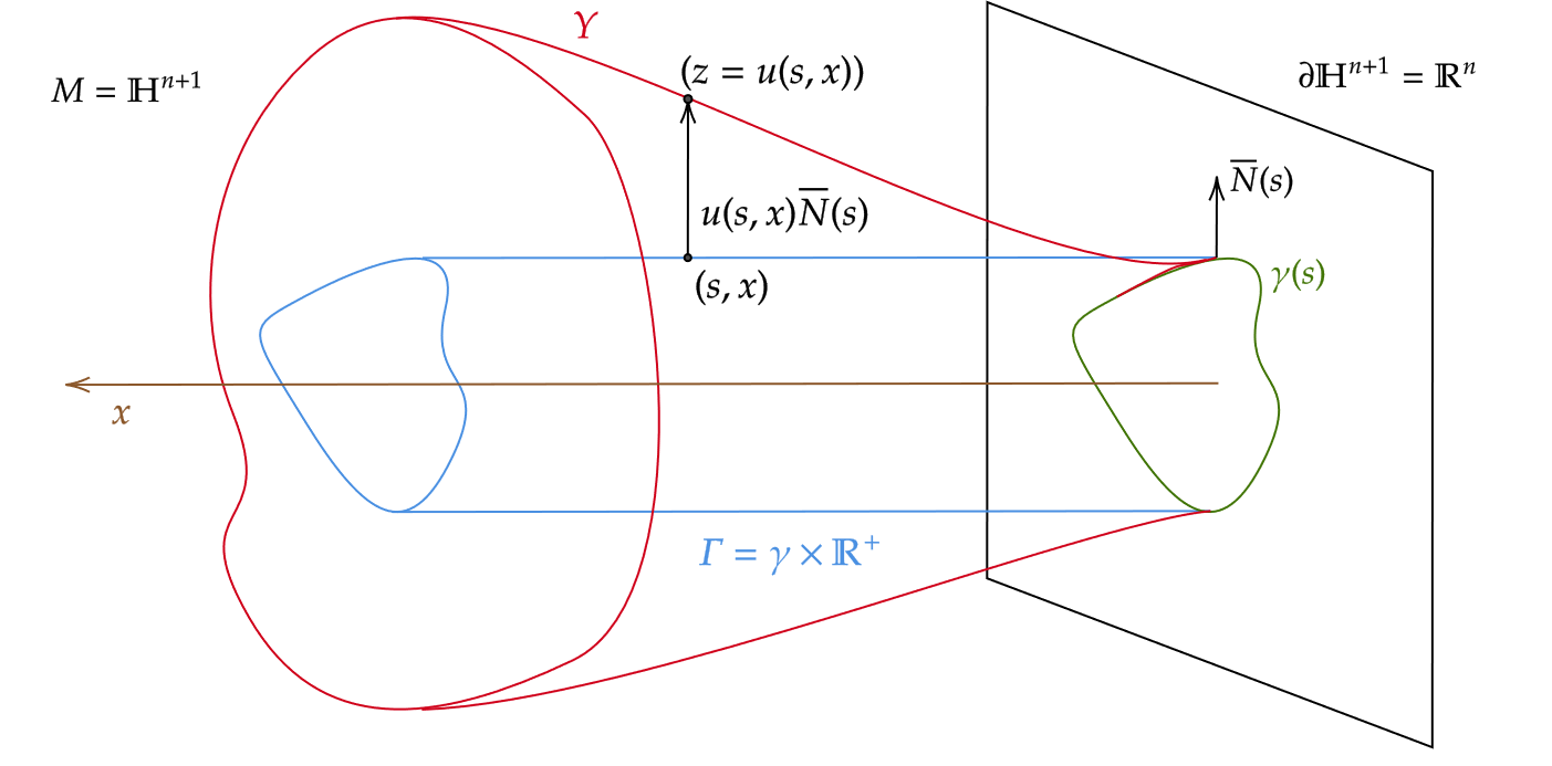
Figure 1:

$u$ satisfies a degenerate elliptic equation coming from $Y$ being minimal. In §3, we establish regularity of $u$ and prove theorem 3.1

Theorem.

For $Y^{m}\subseteq M^{n+1}$ minimal and $u=u^{i}\overline{N}_{i}$ satisfying (1), we have

$$u^{i}(s,x)=\begin{cases}u_{2}^{i}(s)x^{2}+u_{4}^{i}(s)x^{4}+\dots+u^{i}_{m}(s)x^{m}+u^{i}_{m+1}(s)x^{m+1}+\dots&\text{m even}\\[8.61108pt] u_{2}^{i}(s)x^{2}+u_{4}^{i}(s)x^{4}+\dots+u^{i}_{m+1}(s)x^{m+1}+U^{i}(s)x^{m+1}\log(x)+u_{m+2}(s)x^{m+2}+\dots&\text{m odd }\end{cases}$$

for $C^{m+1,\alpha}$ coefficients $u_{k}(s)$ and $U(s)$.

§3 contains the full details. To make similar statements to the above but more concisely, we recall notation from [1]: let

$$f :\Gamma\to\mathbb{R}$$

$$f(s,x) =f_{0}(s)+f_{1}(s)x+\dots+f_{m}(s)x^{m}+O(x^{m+1})$$

and define

$$\mathcal{F} :C^{\infty}(\Gamma)\to\mathbb{Z}$$

$$\mathcal{F}(f) =\begin{cases}0&\text{if $f$ is }O(x^{m+1})\\ 1&\text{if $f$ is even below }x^{m}\text{ and not }O(x^{m+1})\\ -1&\text{if $f$ is odd below }x^{m}\text{ and not }O(x^{m+1})\\ \text{undefined}&\text{else}\end{cases}$$

When $m$ is odd, we define the above but replacing $m\to m+1$ and allowing for $x^{m+1}\log(x)$ terms. We will often omit the case of $\mathcal{F}=0$ and write $\mathcal{F}=1$ or $\mathcal{F}=-1$ for our computations, i.e. any statement of $\mathcal{F}=\pm 1$ should be interpreted as $\mathcal{F}\in\{0,\pm 1\}$ (see §2.5 for a full definition and convention). We note that theorem 3.1 becomes, $\mathcal{F}(u)=1$ (or $\mathcal{F}(u)=0$, implicitly). With this, we informally state theorem 4.1 in codimension $1$

Theorem.

Suppose that $Y^{m}\subseteq M^{n+1}$ minimal with $\overline{h}=\overline{g}\Big{|}_{TY}$ even up to order $x^{m}$. Let $p\in Y$, $\overline{A}:\text{Sym}^{2}(TY)\to N(Y)$ denote the second fundamental form, $\overline{\nu}$ be a normal to $Y$, both with respect to $\overline{g}$. Then $\overline{A}$ and its covariant derivatives are even up to order $x^{m}$.

See §4 for the full theorem. We also consider variations of $Y$ among the space of minimal submanifolds. We can describe a smooth family of minimal submanifolds as

$$Y_{t}=\exp_{Y}(S_{t})$$

for $S_{t}\in N(Y)$ a smooth function of $t$ and $\exp_{Y}$ the exponential map with respect to $h=g\Big{|}_{Y}$. Let $\dot{S}:=F_{*}(\partial_{t})\Big{|}_{t=0}$ and $\ddot{S}=\nabla_{F_{*}(\partial_{t})}F_{*}(\partial_{t})\Big{|}_{t=0}$. Both satisfy Jacobi equations when $\{Y_{t}\}$ is a family of minimal submanifolds, giving regularity and parity. in codimension $1$ we can write

$$\dot{S} =\dot{\phi}(s,x)\overline{\nu}(s,x)$$

$$\ddot{S} =\ddot{\phi}(s,x)\overline{\nu}(s,x)$$

for $\overline{\nu}$ a normal to $Y$ with respect to $\overline{g}$ (see figure 2).

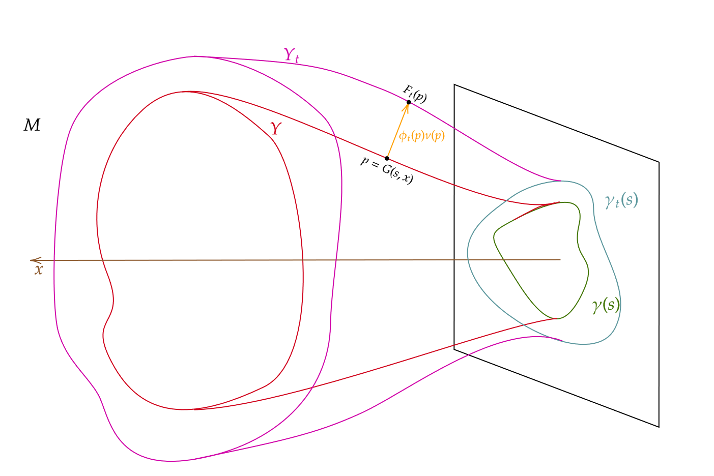
Figure 2:

We informally state theorem 5.1

Theorem.

For $\{Y_{t}\}$ a family of minimal submanifolds, and $\dot{S}=\dot{\phi}(s,x)\overline{\nu}$, $\ddot{S}=\ddot{\phi}\overline{\nu}$:

$$\forall i,\quad\mathcal{F}(\dot{\phi}^{i}) =1$$

$$\forall i,\quad\mathcal{F}(\ddot{\phi}^{i}) =1$$

i.e. $\dot{\phi}$ and $\ddot{\phi}$ are even in $x$ to high order - see section §5 for full details. We remark that in order to compute an equation for $\ddot{S}$, we compute the second variation of mean curvature (i.e. third variation of area). The author was unable to find this result in the literature, so it is stated in proposition 2. In codimension $1$, we get corollary 5

Proposition.

For $\{Y_{t}\}$ a family of minimal submanifolds, and $\dot{S}=\dot{\phi}(s,x)\overline{\nu}$, $\ddot{S}=\ddot{\phi}\overline{\nu}$, we have that

$$\frac{d^{2}}{dt^{2}}H(t)\Big{|}_{t=0} =[J_{Y}(\ddot{\phi})+G(\dot{\phi},\nabla\dot{\phi},D^{2}\dot{\phi})]\nu=0$$

where $\mathcal{F}(G(\dot{\phi},\nabla\dot{\phi},D^{2}\dot{\phi}))=1$

We then compute the first and second variations of renormalized volume in theorem 8.1. In codimension $1$, $n$ even, with $k_{n+1}=0$ (e.g. $M=\mathbb{H}^{n+1}/\Gamma$, see (3)), we get propositions 10.1 10.2

Theorem.

$$\frac{d}{dt}\mathcal{V}(Y_{t})\Big{|}_{t=0} =-(n+1)\int_{\gamma}\dot{\phi}_{0}(s)u_{n+1}(s)\;dA_{\gamma}(s)$$

$$\frac{d^{2}}{dt^{2}}\mathcal{V}(Y_{t})\Big{|}_{t=0} =\int_{\gamma}\Big{(}-(n+1)\ddot{\phi}_{0}u_{n+1}+(1-n)\dot{\phi}_{0}(s)\dot{\phi}_{n+1}(s)$$

$$+\dot{\phi}_{0}(s)^{2}\left[(n-1)(n-2)-4(3n-1)u_{2}u_{n+1}(s)\right]\Big{)}\;dA_{\gamma}(s)$$

The full theorem in arbitrary codimension and $m$ odd is stated in §8. We note that while $M$ being PE is the most natural setting, our results hold for a slightly larger class of manifolds - namely those that are conformally compact with a metric, $g$, that splits as in (2) with $k(x,s)$ satisfying (3).

As an application of the second variation formula and regularity of $u$, we prove the following projection relationship, proposition 3

Theorem.

For $n$ even, $Y^{n}\subseteq\mathbb{H}^{n+1}$ minimal with graphical expansion given by $u(s,x)$, we have

$$\boxed{\frac{\langle u_{2},u_{n+1}\rangle_{L^{2}(\gamma)}}{\text{Vol}(\gamma)}=-\frac{(n-1)(n-2)}{2(n^{2}-6n+1)}}$$

Remark  when $n=2$ we get that $\langle u_{2},u_{3}\rangle_{\gamma}=0$

1.3 Outline of Proofs

This paper has $3$ goals:

• In §3, we show that $Y$ can be described in Fermi coordinates by a graphical function $u$. We prove that $u$ has an even expansion as as we approach the boundary, and that $u$ is highly regular (formally “polyhomogeneous”) in this domain

  • The proof relies on Allard’s regularity theorem, as well as geometric microlocal techniques from [26], and standard PDE arguments. The author suspects that Allard’s theorem can be avoided in establishing the regularity of $Y$, but have yet to find such a proof.

  • Several authors have contributed to the existence, regularity, and asymptotic expansions of minimal hypersurfaces in hyperbolic space, including Lin [21], Guan, Spruck, Szapiel [15], Tonegawa [28], Han, Sehn, Wang [16], and Jiang [19]. These authors primarily use classical PDE techniques, and by contrast, we use methods from geometric microlocal analysis to establish regularity.

  • This immediately shows that $h=g\Big{|}_{Y}$ and $\overline{A}_{Y}$ have corresponding even expansions in $x$ as well

• In §5, we consider a family of submanifolds close to $Y$, $\{Y_{t}\}$ with $Y_{t=0}=Y$. Each $Y_{t}$ can be written as $Y_{t}=\exp_{Y}(S_{t}(p))$ for some $S_{t}\in N(Y)$. We show that $\dot{S}$ and $\ddot{S}$ are regular and admit even asymptotic expansions, by computing the first and second variations of mean curvature.

• In §8 and §9, we prove a formula for the first and second variations of renormalized volume for families of minimal submanifolds $\{Y_{t}\}\subseteq M^{n+1}$. Such formulae appear for minimal surfaces in $\mathbb{H}^{3}$ in [2], and we extend their results to $Y^{m}\subseteq M^{n+1}$ for $m$ and $n$ arbitrary, and $M$ a PE manifold. Past research ([2] [1] [12]) focuses on $m$ even, however we extend our results to $m$ odd as well.

• In §10, we specialize our result to the codimension $1$ case, i.e. $m=n$, yielding a slight correction to the second variation formula in [2]. We use this to prove an $L^{2}$-orthogonality result in §11

The author wishes to thank Rafe Mazzeo for providing the inspiration for this problem, as well as his time spent across many meetings. The author also wishes to thank Otis Chodosh for suggesting the application in §11, as well as Brian White and Joel Spruck, for their insight on barrier arguments for minimal submanifolds.

2 Preliminaries

2.1 Defining Renormalized Volume

Consider $M^{m}$ a Poincare-Einstein manifold. For $x:\overline{M}\to\mathbb{R}^{\geq 0}$ a special bdf, the metric splits in Graham-Lee Normal form as

$$g=\frac{dx^{2}+k(s,x)}{x^{2}}$$ (2)

with $(s,x)$ smooth coordinates on a neighborhood, $U$, of $\partial M$, with $U\cong\partial M\times[0,b)$ for $b>0$. Here, $k(s,x)$ is a smooth tensor on $T\partial M$, i.e. $k(\partial_{x},\cdot)\equiv 0$, and it has an even expansion in $x$ up to order $x^{m-2}$ ($x^{m-1}$) when $m$ is even (odd), i.e.

$$m\text{ even}\implies k(s,x) =k_{0}(s)+x^{2}k_{2}(s)+\dots+k_{m-2}(s)x^{m-2}+k_{m-1}(s)x^{m-1}+k_{m}(s)x^{m}+O(x^{m+1})$$ (3)

$$m\text{ odd}\implies k(s,z,x) =k_{0}+x^{2}k_{2}+\dots+x^{m-1}k_{m-1}+x^{m-1}\log(x)K+x^{m}k_{m}+x^{m+1}k_{m+1}+O(x^{m+2})$$

we then compute

$$d\text{Vol}=\sqrt{\det g}dx\wedge ds=\frac{1}{x^{m}}\sqrt{\det k}\;dx\wedge ds$$

In [9], Graham showed that for $m$ even,

$$q(x,s):=\sqrt{\det k} =q_{0}(s)+q_{2}(s)x^{2}+\dots+q_{m}(s)x^{m}+q_{m+1}(s)x^{m+1}+\dots$$

i.e. $\text{Tr}(k_{m-1})=0$ and $q$ is even up to order $m$. For $m$ even, define

$$\mathcal{V}(M) :=\underset{\epsilon\to 0}{FP}\;\int_{x>\epsilon}d\text{Vol}$$

$$\int_{x>\epsilon}d\text{Vol} =\left(\int_{x>b}+\int_{\epsilon}^{b}\right)\frac{q(x,s)}{x^{m}}dxds$$

$$=\int_{x>b}d\text{Vol}+\int_{x=\epsilon}^{b}[x^{-m}q_{0}(s)+x^{-m+2}q_{2}(s)+\dots+q_{m}(s)+R(s,x)]dsdx$$

$$=I(b)+c_{0}(s)\frac{b^{-m+1}-\epsilon^{-m+1}}{1-m}+\dots+c_{m}(s)(b-\epsilon)+F(b,\epsilon)$$

where $R(s,x)=O(x)$ and

$$F(b,\epsilon) :=\int_{x=\epsilon}^{b}R(s,x)dsdx$$

$$c_{2k}(s) :=\int_{\partial M}q_{2k}(s)ds$$

Renormalized volume is then

$$\mathcal{V}(M) =\underset{\epsilon\to 0}{FP}\;I(b)+\sum_{k=0}^{m/2}c_{2k}(s)\frac{b^{-m+1}-\epsilon^{-m+1}}{1-m}+F(b,\epsilon)$$

$$=I(b)+F(b,0)+\sum_{k=0}^{m/2}c_{2k(s)}\frac{b^{-m+1}}{1-m}$$

A priori, using $x$ seems arbitrary, as there could be several functions like $x$ for which we have an asymptotic expansion in $\epsilon$. Formally, we require $x$ to be a “special bdf” which we define in §2.2. One can show that renormalized volume is a geometrically natural quantity to consider as it is:

• Independent of the parameter $b$

• Independent of the choice of special bdf, $x$, or equivalently independent of the representative in the conformal infinity, $k_{0}=\overline{g}\Big{|}_{\gamma}$

The former fact follows by keeping track of boundary terms when integrating applying the FTC. The latter two facts are discussed in [12] among other sources, and are also shown in §13.6. These properties only hold for $m$ even. Renormalized volume is defined similarly for odd dimensional submanifolds and is done in §13.6. However, the renormalized volume depends on the choice of $x$, and hence depends on the choice of representative of the conformal infinity.

Note that to have an expansion for $k(s,x)$ (and hence $q(s,x)$) in the first place, there needs to be some regularity of the metric as we approach the boundary. When we handle the case of $Y^{m}\subseteq M^{n+1}$ with the metric induced by resstriction, this amounts to regularity of $Y$ itself. Thus, when we prove regularity of $Y$, we implicitly prove that renormalized volume is mathematically defined for our class of $Y^{m}\subseteq M^{n+1}$ minimal.

2.2 Brief Review of Poincaré-Einstein Manifolds

The splitting of the metric in (2) is motivated by Graham-Lee Normal Form [11] [6] for Poincaré-Einstein (PE) manifolds. A Riemannian manifold $(M,g)$ is Einstein if $g$ satisfies the Einstein equations. The manifold is Poincare if $g$ is conformally compact, i.e. the boundary is compact and there exists a function

$$\rho:\overline{M}\to\mathbb{R}^{\geq 0}\qquad\text{ s.t. }\qquad\{\rho=0\}=\partial M,\qquad\overline{\nabla}\rho|_{\partial M}\neq 0$$

and $\overline{g}=\rho^{2}g$ is a nondegenerate metric on $\overline{M}$. Here, $\overline{\nabla}:=\nabla^{\overline{g}}$ and we call $\overline{g}:=\rho^{2}h$ the compactified metric. Furthermore, $\rho$ is a boundary defining function (bdf). We are interested in $\overline{g}|_{\partial M}$ and how it determines $\overline{g}$ on the interior. Note that if $\varphi:\overline{M}\to\mathbb{R}^{+}$ is a positive smooth function, then $\tilde{\rho}=\varphi\rho$ is also a boundary defining function. As a result, we can consider the conformal class $[\overline{g}|_{\partial M}]$, which we call the conformal infinity. For PE manifolds with a chosen representative, $k_{0}$, in the conformal infinity, there exists a bdf $x$, for which $\overline{g}$ splits as in equation 2. Moreover, $k(s,x)$ is regular up to order $x^{m}$ as shown in [11]. The bdf $x$ is special if

$$||d\log(x)||_{g}=1$$

holds in a neighborhood of $\partial M$. Furthremore, by equation (2) we have $k_{0}=x^{2}g\Big{|}_{\partial M}$. Given these conditions, $x$ is unique (see [5] for details). Renormalized volume is conformally invariant for $m$ even in the sense that it does not depend on the choice of $k_{0}\in[\overline{g}|_{\partial M}]$ and the corresponding special bdf used. Thus, we can define renormalized volume for $m$ even as long as we use a special bdf (see [1] [12]).

Example.

Consider the Poincare Ball model of hyperbolic space $M=\mathbb{H}^{3}$. The metric on $\mathbb{H}^{3}$ is

$$g=\frac{4}{(1-r^{2})^{2}}\left[dr^{2}+r^{2}d\phi^{2}+r^{2}\sin^{2}\phi d\theta^{2}\right]$$

is Einstein. We want to find a special bdf, $\rho$, for $\mathbb{H}^{3}$. We assume that it is rotationally symmetric, i.e. $\rho_{\theta}=\rho_{\phi}=0$. With this, we compute

$$1=||d\log(\rho)||_{g}^{2}=\frac{\rho_{r}^{2}}{\rho^{2}}g^{rr}=\partial_{r}(\log(\rho))^{2}\frac{(1-r^{2})^{2}}{4}$$

we take the negative root and get

$$\partial_{r}(\log(\rho))=\frac{-2}{1-r^{2}}$$

Integrating and exponentiating, we compute

$$\rho=A\frac{1-r}{1+r}$$

for $0\leq r\leq 1$ and some constant $A$. Note that as long as $A\neq 0$, we have $\rho^{-1}(0)=\{r=1\}=S^{2}$, which is the boundary of $\overline{\mathbb{H}^{3}}$. Suppose that we want to prescribe the standard metric on this boundary. i.e. $k_{0}(\theta)=\sin^{2}\phi d\theta^{2}+d\phi^{2}$. Then we have that

$$k_{0}=\rho^{2}h\Big{|}_{r=1}=\frac{4A^{2}}{(1+r)^{4}}[dr^{2}+r^{2}d\phi^{2}+r^{2}\sin^{2}\phi d\theta^{2}]\Big{|}_{r=1}=\frac{4A^{2}}{16}[d\phi^{2}+\sin^{2}\phi d\theta^{2}]$$

so we choose $A=2$ so that $\rho$ is positive. Se see that $\overline{g}\Big{|}_{r=1}=\overline{g}\Big{|}_{\partial M}=k_{0}$. Note that

$$\overline{\nabla}\rho =\overline{g}^{ij}(\partial_{i}\rho)\partial_{j}=\overline{g}^{rr}(\partial_{r}\rho)\partial_{r}=\frac{(1+r)^{4}}{16}\cdot\frac{-4}{(1+r)^{2}}\partial_{r}$$

$$\overline{\nabla}\rho\Big{|}_{r=1} =-\partial_{r}$$

which is non-zero.

We can also compute the renormalized volume of $Y=\mathbb{H}^{2}\subseteq\mathbb{H}^{3}=M$ in this model.

Example.

Consider the Poincare Ball model of hyperbolic space with $\mathbb{H}^{2}\subseteq\mathbb{H}^{3}$ represented as the geodesic disk (see figure 3). The restricted metric on $\mathbb{H}^{2}$ corresponds to when $\phi=\pi/2$

$$h:=g\Big{|}_{\mathbb{H}^{2}}=\frac{4}{(1-r^{2})^{2}}[dr^{2}+r^{2}d\theta^{2}]$$

Because $\rho=\frac{2(1-r)}{1+r}$ is rotationally symmetric, it is the special bdf for $\mathbb{H}^{2}$ by the same computation.

Figure 3: Poincare Ball model framed as PE manifold, with $\mathbb{H}^{2}$ submanifold

With this, we can compute the renormalized area of $\mathbb{H}^{2}\subseteq\mathbb{H}^{3}$

$$\mathcal{V}(\mathbb{H}^{2}) =\underset{\epsilon\to 0}{FP}\;\int_{\rho>\epsilon}dA=\underset{\epsilon\to 0}{FP}\;\int_{\rho>\epsilon}\frac{4r}{(1-r^{2})^{2}}drd\theta$$

$$=\underset{\epsilon\to 0}{FP}\;4\pi\int_{r=0}^{(2-\epsilon)/(2+\epsilon)}\frac{d}{dr}\frac{1}{1-r^{2}}dr$$

since $\rho>\epsilon\leftrightarrow\frac{2-\epsilon}{2+\epsilon}>r$. Integrating, we get

$$\int_{\rho>\epsilon}dA=4\pi\left[(1-r^{2})^{-1}\right]_{r=0}^{(2-\epsilon)/(2+\epsilon)}=4\pi\left[\frac{4+4\epsilon+\epsilon^{2}}{8\epsilon}-1\right]=4\pi\left[\frac{1}{2\epsilon}-\frac{1}{2}+\frac{\epsilon}{8}\right]$$

Taking the constant term in $\epsilon$ then yields

$$\underset{\epsilon\to 0}{FP}\;\int_{\rho>\epsilon}dA=4\pi\cdot\frac{-1}{2}=\boxed{-2\pi}$$

This example generalizes to higher dimensions as well.

2.3 Model Case: Half Space Model of $\mathbb{H}^{n+1}$

Consider $\mathbb{H}^{n+1}$ now with the half-space structure. The metric is

$$g=\frac{dx^{2}+(dy_{1}^{2}+\dots+dy_{n}^{2})}{x^{2}}$$

so that $k(s,x)$ is the standard Euclidean metric on the first $n$ coordinates, which is even in $x$ as there is no $x$ dependence. Clearly the metric splits in the desired form, and

$$||d\log(x)||_{g}^{2}=g^{xx}\partial_{x}(\log(x))^{2}=x^{2}\cdot(1/x)^{2}=1$$

Moreover the chosen representative of the conformal infinity is

$$k_{0}=dy_{1}^{2}+\dots+dy_{n}^{2}=x^{2}g\Big{|}_{x=0}$$

where we take $\mathbb{R}^{n}=\partial\mathbb{H}^{n+1}$. The issue is that the boundary is not compact. In order for this to be a conformally compact manifold, we need to consider the one point compactification of $\mathbb{R}^{n}$ as the boundary, i.e. $S^{n}$, and redefine the metric appropriately. Under this compactification, $x$ is no longer a bdf because of the added point at infinity which would have $x=+\infty$ as opposed to $x=0$.

Conformally compact minimal submanifolds of $\mathbb{H}^{n+1}$   Despite the above, our analysis in this paper is motivated and includes $M=\mathbb{H}^{n+1}$ with the half space model. Though $x$ is not a valid bdf for $\mathbb{H}^{n+1}$ itself, it can be used to define renormalized volume for minimal submanifolds with compact boundary (which are conformally compact) that are smoothly embedded in a neighborhood of the boundary. We have $\partial Y=\gamma\subset\subset\mathbb{R}^{n}=\partial\mathbb{H}^{n+1}$ so $x\Big{|}_{Y}(p)=0\iff p\in\gamma$. This means that $x\Big{|}_{Y}$ does define the boundary. However, even if

$$||d\log(x)||_{g}=1$$

it is not usually true that $||d\log(x)||_{h}=1$ for the induced metric $h=g\Big{|}_{Y}$. Moreover, the metric may not split, i.e. $h(\partial_{s_{a}},\partial_{x})\neq 0$. To get around this, the idea is as follows: $Y$ is quadratic and even to high order as we approach the boundary (see 3.1). As a result, if we consider a special bdf for $Y$, call it $x_{Y}$, we can write it in a neighborhood of the boundary as

$$x_{Y}=xe^{\omega(s,x)}$$

where $\omega(s,0)=0$ and $\omega(s,x)$ has an even expansion up to order $m+2$ (see §7). Consequently $k(s,x)$ still has an even expansion up to order $m$ in equation (2), so it makes sense to define

$$\mathcal{V}(Y)=\underset{\epsilon\to 0}{FP}\;\int_{\{x_{Y}>\epsilon\}\cap Y}dA$$

and it turns out that

$$\underset{\epsilon\to 0}{FP}\;\int_{\{x>\epsilon\}\cap Y}dA=\underset{\epsilon\to 0}{FP}\;\int_{\{x_{Y}>\epsilon\}\cap Y}dA$$

by parity considerations. To formally show this, we first introduce Riesz regularization in §2.4, we then reprove the fact that Riesz regularization produces the result as Hadamard regularization in §13.6, and finally, we show that the usage of $x$ vs. $x_{Y}$ is irrelevant in defining renormalized volume for minimal submanifolds in $\mathbb{H}^{n+1}$ in §7. It is also worth noting that while we consider $M$ a PE space more generally, our analysis of $Y\subseteq M$ is local near a point $p\in\partial Y=\gamma$, for which we can choose coordinate charts resembling hyperbolic space.

Example.

Consider the geodesic copy of $\mathbb{H}^{2}$ as a hemisphere of radius $1$ inside $\mathbb{H}^{3}=\{(x,y,z)\;|\;x\geq 0\}$ with the metric $\frac{dx^{2}+dy^{2}+dz^{2}}{x^{2}}$. The boundary is a circle of radius $1$, and we parameterize $\mathbb{H}^{2}$ as

$$f(x,\theta)=(x,\sqrt{1-x^{2}}\cos\theta,\sqrt{1-x^{2}}\sin\theta)$$

we compute the induced metric

$$h_{xx} =g(f_{x},f_{x})=\frac{1}{x^{2}(1-x^{2})}$$

$$h_{x\theta} =g(f_{x},f_{\theta})=0$$

$$h_{\theta\theta} =g(f_{\theta},f_{\theta})=\frac{1-x^{2}}{x^{2}}$$

so that

$$dA_{\mathbb{H}^{2}}=\sqrt{\det g}dxd\theta=\frac{1}{x^{2}}dxd\theta$$

we now compute

$$\mathcal{V}(\mathbb{H}^{2})=\underset{\epsilon\to 0}{FP}\;\int_{x>\epsilon}dA_{\mathbb{H}^{2}}$$

we integrate

$$\int_{x>\epsilon}dA_{\mathbb{H}^{2}}=\int_{\theta=0}^{2\pi}\int_{x=\epsilon}^{1}\frac{1}{x^{2}}dxd\theta=2\pi\left[-\frac{1}{x}\right]_{\epsilon}^{1}=-2\pi+\frac{2\pi}{\epsilon}$$

and so $\mathcal{V}(\mathbb{H}^{2})=\boxed{-2\pi}$, which is the same result as if we computed the renormalized volume in the “proper” setting, i.e. the ball model.

2.4 Riesz Regularization

Having defined special bdfs, we can define renormalized volume in an alternate way with Riesz regularization: given an asymptotically hyperbolic manifold, $M$, and a special bdf, $x_{M}$, on $M$, consider the following meromorphic function

$$f(z)=\int_{M}x_{M}^{z}dA_{M}$$

As with Hadamard regularization, the quantity $x_{M}$ seems unmotivated. However, $x_{M}$ being a special bdf gives $f(z)$ geometric meaning. This function is holomorphic for $\text{Re}(z)>m$, and it has poles at $z\in\{-\infty,\dots,-1,0,1,\dots,m\}$. We define

$$\mathcal{V}(M):=\underset{z=0}{FP}\;\int_{M}x^{z}dA_{M}=\underset{z=0}{FP}\;f(z)$$

Computing $\underset{z=0}{FP}\;f(z)$ amounts to subtracting off the pole at $z=0$ (if it exists) and evaluating the remaining difference. This process is known as Riesz regularization, and the equivalence of these two definitions is given in the appendix §13.6. As mentioned before, one can show that for $Y^{m}\subseteq M^{n+1}$ with $Y$ conformally compact and $m<n+1$:

$$\underset{z=0}{FP}\;\int_{Y}x_{Y}^{z}dA_{Y}=\underset{z=0}{FP}\;\int_{Y}x^{z}dA_{Y}$$ (4)

On the left hand side, we are using $x_{Y}$, a special bdf for $Y$ considered as its own asymptotically hyperbolic manifold. On the right hand side, we use $x$, which is a special bdf on $M^{n+1}$. This equation holds for $m$ even, and it holds up to a boundary error for $m$ odd (see §7). The latter is expected, as renormalized volume in odd dimensional manifolds depends on the choice of special bdf ([1]).

Example.

We compute $\mathcal{V}(\mathbb{H}^{2})$ for $\mathbb{H}^{2}\subseteq\mathbb{H}^{3}$ using Riesz regularization in the half space model (we leave it to the reader to compute this for the poincare ball model).

$$\zeta(z)=\int_{\mathbb{H}^{2}}x^{z}dA_{\mathbb{H}^{2}}=\int_{x=0}^{1}\int_{\theta=0}^{2\pi}x^{z-2}dxd\theta=2\pi\left[\frac{x^{z-1}}{z-1}\right]_{x=0}^{x=1}=2\pi\frac{1}{z-1}$$

Again, when we find the meromorphic extension, we first assume $\text{Re}(z)\gg 0$ so that $0^{z-1}=0$. There is no pole at $z=0$ in this extension, so

$$\mathcal{V}(\mathbb{H}^{2})=\underset{z=0}{FP}\;\zeta(z)=\zeta(0)=\boxed{-2\pi}$$

2.5 Parity of functions

Throughout this paper, we will use $x$ to denote a special bdf on our ambient PE space $(M^{n+1},g)$ and identify a neighborhood of the boundary, $U(\partial M)$, with $\partial M\times[0,\epsilon)$. When $M=\mathbb{H}^{n+1}$, $x$ is the distinguished direction in the decomposition of $\mathbb{H}^{n+1}\cong\mathbb{R}^{n}\times\mathbb{R}^{+}$. Let $f$ be a function defined on $\Gamma\subseteq M$ in coordinates of $(s,x)$. Further assume that $f$ is polyhomogeneous and can be expanded as

$$f(s,x)=\begin{cases}f_{0}(s)+f_{1}(s)x+\dots+f_{m}(s)x^{m}+O(x^{m+1})&m\text{ is even }\\ f_{0}(s)+f_{1}(s)x+\dots+f_{m+1}(s)x^{m+1}+F(s)x^{m+1}\log(x)+O(x^{m+2})&m\text{ is odd }\end{cases}$$ (5)

then we define for $m<n$ even

$$\mathcal{F}(f)=\begin{cases}0&f(s,x)\text{ is }O(x^{m+1})\\ 1&f(s,x)\text{ is even up to }x^{m}\text{ and not }O(x^{m+1})\\ -1&f(s,x)\text{ is odd up to }x^{m}\text{ and not }O(x^{m+1})\\ \text{undefined}&\text{else}\end{cases}$$ (6)

When $m=n$, we assume that

$$f(s,x)=\begin{cases}f_{0}(s)+f_{1}(s)x+\dots+f_{m}(s)x^{m}+F(s)x^{m}\log(x)+O(x^{m+1})&m\text{ is even }\\ f_{0}(s)+f_{1}(s)x+\dots+f_{m+1}(s)x^{m+1}+F(s)x^{m+1}\log(x)+O(x^{m+2})&m\text{ is odd }\end{cases}$$ (7)

For $m=n$ even, we define

$$\mathcal{F}(f)=\begin{cases}0&f(s,x)\text{ is }O(x^{n+1})\\ 1&f(s,x)\text{ is even up to }x^{n}\log(x)\text{ and not }O(x^{n+1})\\ -1&f(s,x)\text{ is odd up to }x^{n}\log(x)\text{ and not }O(x^{n+1})\\ \text{undefined}&\text{else}\end{cases}$$ (8)

Similarly for $m=n$ odd, we define

$$\mathcal{F}(f)=\begin{cases}0&f(s,x)\text{ is }O(x^{n+2})\\ 1&f(s,x)\text{ is even up to order }x^{n+1}\log(x)\text{ and not }O(x^{n+2})\\ -1&f(s,x)\text{ is odd up to order }x^{n+1}\log(x)\text{ and not }O(x^{n+2})\\ \text{undefined}&\text{else}\end{cases}$$ (9)

We note that $\mathcal{F}$ is multiplicative in the sense that if $f$ and $g$ both satisfy equation (5) then

$$\mathcal{F}(fg)=\mathcal{F}(f)\mathcal{F}(g)$$

We may explicitly write that a given function is “even/odd up to” a given order when relevant. We are primarily interested in the case of $\mathcal{F}\neq 0$ for all usages of the $\mathcal{F}$ functional. Thus, throughout this paper, any computation of $\mathcal{F}=1$ signifies $\mathcal{F}\in\{0,1\}$, and similarly $\mathcal{F}=-1$ signifies $\mathcal{F}\in\{0,-1\}$. We adopt this convention for brevity at the expense of some clarity. If there are asymptotics to show that $\mathcal{F}\neq 0$, we will write these explicitly.

Remark  The case of $m=n$ even is special because of (3) for $M^{n+1}$

$$\text{$n+1$ even}\implies k(s,x) =k_{0}+x^{2}k_{2}+\cdots+k_{n-1}x^{n-1}+k_{n}x^{n}+k_{n+1}x^{n+1}+O(x^{n+2})$$

$$\text{$n+1$ odd}\implies k(s,x) =k_{0}+x^{2}k_{2}+\cdots+k_{n}x^{n}+Kx^{n}\log(x)+k_{n+1}x^{n+1}+O(x^{n+2})$$

When $Y^{m}\subseteq M^{n+1}$ with $m<n$, we expect the presence of $k_{n-1}x^{n-1}$ in the even case and $Kx^{n}\log(x)$ in the odd case to not affect our formulation of even expansions up to order $m$. However, when $m=n$ even, we expect $K=K(s)$ to give rise to $x^{n}\log(x)$ terms. We note that when $K\equiv 0$, this separate definition for $\mathcal{F}$ when $m=n$ even is unecessary. In particular, for $M=\mathbb{H}^{n+1}/\Gamma$ for $\Gamma$ a coconvex compact subgroup, no $x^{n}\log(x)$ term is present and (6) applies for all $m<n+1$ even.

We also define a parity preserving first order linear operator $L$ as

$$L :=d^{a}(s,x)\partial_{s_{a}}+d^{x}(s,x)\partial_{x}$$ (10)

$$\mathcal{F}(d^{a}) =1$$

$$\mathcal{F}(d^{x}) =-1$$

$$\implies\mathcal{F}(L) =1$$ (11)

We similarly define a parity preserving first order quadratic differential functional, $Q$, as

$$Q(f,g) :=d^{ab}(s,x)f_{a}g_{b}+d^{ax}f_{a}g_{x}+d^{xx}f_{x}g_{x}$$

$$\mathcal{F}(d^{ab}) =1$$

$$\mathcal{F}(d^{ax}) =-1$$

$$\mathcal{F}(d^{xx}) =1$$

$$\implies\mathcal{F}(Q) =1$$

Higher order parity preserving linear operators and quadratic functionals are defined analogously

2.6 Variation of Renormalized Volume

When computing the variation of the renormalized volume, we consider $\{Y_{t}^{m}\}\subseteq M^{n+1}$, a one-parameter family of minimal submanifolds with $Y_{t=0}=Y$ our designated submanifold. We require that each $Y_{t}$ be embedded in some neighborhood of the boundary $\mathcal{U}\cong\partial M\times[0,\epsilon)$. Define

$$S_{t} :Y\to N(Y),\qquad \dot{S} :=\partial_{t}S_{t}\Big{|}_{t=0}$$

$$F_{t} :Y\to Y_{t},\qquad F_{t}(p) :=\exp_{p}(S_{t}(p))$$

Given that this is a variation among minimal submanifolds, we know that $\dot{S}$ lies in the kernel of the Jacobi operator of $N(Y)$, i.e.

$$J_{Y}^{\perp}(\dot{S})=\Delta_{Y}^{\perp}(\dot{S})+\tilde{A}(\dot{S})+\text{Tr}[R_{M}(\cdot,\dot{S})\cdot]=0$$

where $\tilde{A}$ is the Simons operator and $\text{Tr}[R_{M}(\cdot,\dot{S})]$ denotes the trace of the ambient Riemann curvature tensor, $R_{M}$, taken over $TY$, applied to $\dot{S}$. As a result, $\dot{S}$ satisfies a regularity theorem stated in full in §5.1. In codimension $1$, $\dot{S}=\dot{\phi}(s,x)\overline{\nu}(s,x)=[x^{-1}\dot{\phi}(s,x)]\nu$ for $\nu$ a normal to $Y$. Then

$$\forall i,\quad\mathcal{F}(\dot{\phi}^{i})=1$$

i.e. $\dot{\phi}$ is even to $x^{n}$ or $x^{n+1}$ with the presence of a log term when $n$ is odd. Similarly, we show in the appendix that $\ddot{S}$ satisfies an equation of the form

$$J_{Y}^{\perp}(\ddot{S})=Q^{\perp}(\dot{S},\dot{S})$$

where $Q^{\perp}$ is a quadratic functional in $\{\dot{S}^{i},\dot{S}^{i}_{\alpha},\dot{S}^{i}_{\alpha\beta}\}$ valued in $NY$. This establishes regularity in a very similar manner and proves

$$\forall i,\quad\mathcal{F}(\ddot{\phi}^{i})=1$$

In the codimension $1$ even case, neither $\dot{\phi}$ nor $\ddot{\phi}$ have $x^{n}\log(x)$ terms and the details are done in section §13.10. Having established regularity of $\dot{S}$ and $\ddot{S}$, we define

$$\mathcal{V}(Y_{t})=\underset{z=0}{FP}\;\int_{Y_{t}}x^{z}dA_{t}=\underset{z=0}{FP}\;\int_{Y}F_{t}^{*}(x)^{z}F_{t}^{*}(dA_{t})$$

Computing variations of this amounts to differentiating the integrand and interpreting it geometrically in terms of $u(s,x)$, $\dot{S}$, and $\ddot{S}$. When differentiating $\mathcal{V}(Y_{t})$, we must justify the interchange of integration and differentiation, as shown in §13.6.

With this, we state formulae for the first and second variations of renormalized volume in codimension $1$. The full theorem is stated in §8, theorem 8.1.

Theorem.

For $\{Y_{t}^{n}\}\subseteq M^{n+1}$ a one-parameter family of hypersurfaces satisfying mild geometric constraints, suppose $Y_{t=0}=Y$ is minimal with $\partial Y=\gamma$. Then

$$n\;\text{even}\; \implies\frac{d}{dt}\mathcal{V}(Y_{t})\Big{|}_{t=0}=-(n+1)\int_{\gamma}\dot{\phi}_{0}(s)u_{n+1}(s)\;dA_{\gamma}(s)$$

$$n\;\text{odd}\; \implies\frac{d}{dt}\mathcal{V}(Y_{t})\Big{|}_{t=0}=-(n+1)\int_{\gamma}\left[\dot{\phi}_{0}(s)u_{n+1}(s)+F(\dot{\phi}_{0},u_{2})(s)\right]dA_{\gamma}(s)$$

where $F$ is a polynomial in $\dot{\phi}_{0}$, $u_{2}$, and their higher derivatives. If in addition each $Y_{t}$ is minimal, then we have

$$n\;\text{even}\;\implies\frac{d^{2}}{dt^{2}}\mathcal{V}(Y_{t})\Big{|}_{t=0} =\int_{\gamma}-(n+1)\ddot{\phi}_{0}u_{n+1}+(1-n)\dot{\phi}_{0}(s)\dot{\phi}_{n+1}(s)$$

$$+\dot{\phi}_{0}(s)^{2}\left[(n-1)(n-2)-4(3n-1)u_{2}u_{n+1}(s)+\text{Tr}_{T\gamma}(k_{n+1,0})\right]\;dA_{\gamma}(s)$$

$$n\;\text{odd}\;\implies\frac{d^{2}}{dt^{2}}\mathcal{V}(Y_{t})\Big{|}_{t=0} =\int_{\gamma}-(n+1)\ddot{\phi}_{0}u_{n+1}+(1-n)\dot{\phi}_{0}(s)\dot{\phi}_{n+1}(s)$$

$$+\dot{\phi}_{0}(s)^{2}\left[(n-1)(n-2)-4(3n-1)u_{2}u_{n+1}(s)+\text{Tr}_{T\gamma}(k_{n+1,0})\right]$$

$$-\dot{\phi}_{0}(s)\left[4(n+2)\dot{\phi}_{0}(s)u_{2}(s)U(s)+\dot{\Phi}(s)\right]+F_{2}(\ddot{\phi}_{0},\dot{\phi}_{0},u_{2})\;dA_{\gamma}(s)$$

where $k_{n+1,0}(s)=k_{n+1}(s,0)$ in (3)

3 Graphical Asymptotic Expansion

3.1 Results about $u$

In this section, we leverage the fact that $Y$ is minimal and smoothly embedded in a neighborhood of the boundary to get a polyhomogeneous expansion of each $u^{i}$ for $u(s,x)=(u^{1}(s,x),\dots,u^{n-m+1}(s,x))\in N(\Gamma)$. Recall that $u$ is polyhomogeneous if

$$u(s,x)\sim\sum_{\text{Re}(z_{j})\to\infty}\sum_{t=0}^{N_{j}}x^{z_{j}}\log(x)^{t}a_{j,t}(s)\;\;\text{ s.t. }\;\;a_{j,t}\in C^{\infty}(\gamma)$$

To show polyhomogeneity we establish some initial regularity. We assume that as $x\to 0$, the blown up localized mass of $Y$ approaches $1$. Formally, let $x_{0}\ll 1$, $s_{0}\in\gamma$, and define

$$F_{0}:=(s,x,z)\to(\sigma,\xi,\eta):=\left(\frac{s-s_{0}}{x_{0}},\frac{x}{x_{0}},\frac{z-u(s_{0},x_{0})}{x_{0}}\right)$$ (12)

When $M=\mathbb{H}^{n+1}$, $F_{0}$ is an isometry.

Assumption.

For $Y^{m}\subseteq M^{n+1}$ minimal, let $Y_{0}=F_{0}(Y)$. Assume

$$\forall\delta>0,\quad\exists x^{*}>0,\quad\text{ s.t. }\quad \forall x_{0}<x^{*}$$

$$\omega_{m}^{-1}\rho^{-m}||V_{Y_{0},x_{0}^{-2}F_{0}^{*}(\overline{g})}||(B_{\rho}(a)) \leq 1+\delta$$ (13)

for all $a\in B_{x_{0}}((s_{0},x_{0}))$. Here, $\omega_{m}$ is the volume of the $m$-dimensional Euclidean ball of radius $1$, and $||\overline{V}_{Y_{0},x_{0}^{-2}F_{0}^{*}(\overline{g})}||(B_{\rho}(a))$ denotes the mass of the varifold intersected with a small ball with respect to the metric $x_{0}^{-2}F_{0}^{*}(\overline{g})$.

This geometric constraint requires that our minimal surfaces “flatten” out as we blow up near the boundary. This restriction is stronger than what is needed to apply Allard regularity, but it gives the correct $C^{1,\alpha}$ norm bounds. The author hopes that this can be proven with a weaker assumption. With this, we state our regularity theorem.

Theorem 3.1.

Suppose $Y^{m}\subseteq M^{n+1}$ minimal satifying equation (13) and $\gamma=\partial Y=Y\cap\partial M^{n+1}$ is a $C^{m+1,\alpha}$ embedded submanifold in $\partial M^{n+1}$. Further suppose that $Y$ is embedded and graphical in some neighborhood of the boundary $\mathcal{U}\cong\partial M\times[0,\epsilon)$. Let $u(s,x)=u^{i}(s,x)\partial_{z_{i}}\in N(\Gamma)$, which describes $Y$ as in §3.2. Then, each $u^{i}(s,x)$ is polyhomogeneous and even to order $m$ ($m+1$) for $m$ even (odd).

$$u^{i}(s,x)=\begin{cases}u_{2}^{i}(s)x^{2}+u_{4}^{i}(s)x^{4}+\dots+u^{i}_{m}(s)x^{m}+u^{i}_{m+1}(s)x^{m+1}+O(x^{m+2}\log(x))\text{m even}\\[8.61108pt] u_{2}^{i}(s)x^{2}+u_{4}^{i}(s)x^{4}+\dots+u^{i}_{m+1}(s)x^{m+1}+U^{i}(s)x^{m+1}\log(x)+O(x^{m+2}\log(x))&\text{m odd }\end{cases}$$

Here, $\{\partial_{z_{i}}\}$ is a coordinate basis for $N(\Gamma)$, and $u^{i}_{k}(s)$, $U^{i}(s)$ are $C^{m+1,\alpha}$ functions on $\gamma$.

Remark  This theorem justifies the existence of an asymptotic expansion for $u$, the graphical function of $Y$, as in [12].

There are several steps to the proof, which we carry out in the following sections:

1. In §3.4, we use the maximum principle and the fact that $Y$ is minimal to show that $u$ is $O(x^{2})$.

2. In §3.5, we use Allard’s regularity theorem and assumption (13) to establish $u\in C_{0}^{1,\alpha}$. We then use the theory of edge operators as in [26] to prove that $u$ is infinitely regular with respect to edge operators.

3. In §3.5.2 we note that $Y$ is minimal so $u$ also satisfies a degenerate elliptic PDE. We reframe the PDE in terms of the $0$-operators, $(x\partial_{x})$ and $(x\partial_{s_{a}})$.

4. In §3.6, we upgrade regularity in $0$-operators to regularity in $b$-operators, $\{x\partial_{x},\partial_{s_{a}}\}$.

5. In §3.8, we upgrade regularity in $b$-operators to $u$ having a polyhomogeneous expansion using a power series iteration in $x$. This follows by linearizing the minimal surface system about successive iterations of $u$, i.e. $u=0$, $u=u_{2}x^{2}$, $u=u_{2}x^{2}+u_{4}x^{4}+\dots$.

As remarked in the previous section, the regularity of $Y$ allows us to formally define renormalized volume

Corollary 3.1.1.

For $Y^{m}\subseteq M^{n+1}$ as above with $m$ even, the renormalized volume

$$\mathcal{V}(Y):=\underset{\epsilon\to 0}{FP}\;\int_{x>\epsilon}dA_{Y}=\underset{z=0}{FP}\;\int_{Y}x^{z}dA_{Y}$$

is formally defined and independent of the special bdf $x$. For $m$ odd, $\mathcal{V}(Y)$ is defined as above, but it depends on the choice of $x$.

3.2 Coordinates and Notation

We coordinatize our space as follows: let $p\in\gamma$ be labeled by geodesic normal coordinates on $\gamma$ about some base point $p_{0}$, i.e.

$$p=f(s):=\overline{\exp}_{p_{0}}^{\gamma}(s^{a}E_{a})$$ (14)

where $\{E_{a}\}$ is an ONB at $p_{0}$ spanning $T_{p_{0}}\gamma$. We then map to the cylinder

$$R(s,x)=(f(s),x)\in\partial M\times[0,\epsilon)$$

where we implicitly use the diffeomorphism of $\partial M\times[0,\epsilon)\cong U\subseteq\overline{M}$ for an open neighborhood of the boundary. We define

$$F(s,x,z)=\overline{\exp}^{\Gamma}_{R(s,x)}(z^{i}X_{i})$$

where $z=(z_{1},\dots,z_{n-m+1})$ are coordinates for the normal bundle, $N\Gamma$, and $\{X_{i}\}$ is an ONB at $p=R(s,x)$. Note that in both instances, $\overline{\exp}$ denotes the exponential map with respect to the compactified metric, $\overline{g}$, restricted to $\gamma$ and $\Gamma$, respectively. We coordinatize $Y$, in some neighborhood of the cylinder $\Gamma$, via

$$Y\in q=F(s,x,u(s,x))\leftrightarrow(s,x,z=u(s,x))$$

for $||s||$ close to $0$ and $x<\epsilon$. This is the definition of the function $u(s,x)$ as an $m$-vector in $N(\Gamma)$, and we investigate this function in the next section.

Finally, we will use $v_{(\cdot)},\;\partial_{(\cdot)}$ to denote a variety of vectors in $TM=TY\oplus NY=T\Gamma\oplus N\Gamma$. Here, we notate

$$\begin{gathered}a,b,c,d\leftrightarrow s_{a},s_{b},s_{c},s_{d}\\ i,j,k,\ell\leftrightarrow z_{i},z_{j},z_{k},z_{\ell}\\ i,j,k,\ell\leftrightarrow w_{i},w_{j},w_{k},w_{\ell}\\ \alpha,\beta,\gamma,\delta\leftrightarrow\{y_{\alpha},y_{\beta},y_{\gamma},y_{\delta}\}\subseteq\{s_{a},x\}\\ \sigma,\mu,\nu,\tau,\omega\leftrightarrow\{y_{\sigma},y_{\mu},y_{\nu},y_{\tau},y_{\omega}\}\subseteq\{s_{a},x,z_{i}\}\end{gathered}$$ (15)

We recognize the abuse of notation between the $i,j,k,\ell$. The context will be clear when using these indices to refer to the fermi normal frame off of $\Gamma$, i.e. $\{\partial_{z_{i}}\}$, vs. the normal frame off of $Y$, $\{w_{i}\}$, defined in section §13.3

3.3 Metric on $Y$

We have the coordinate representation

$$G(s,x):=(F(s,u(s,x)),x)=(s,z=\vec{u}(s,x),x)\leftrightarrow p\in Y$$ (16)

for $G:\Gamma\to Y$. We define

$$v_{a} =G_{*}(\partial_{s_{a}})$$

$$v_{x} =G_{*}(\partial_{x})$$

$$v_{\alpha},v_{\beta},v_{\gamma},v_{\delta} \in\{v_{a},v_{x}\}$$

$$v_{\sigma},v_{\mu},v_{\nu},v_{\tau},v_{\omega} \in\{v_{a},v_{x},w_{i}\}$$

where $\{w_{i}\}$ is the aforementioned normal frame. We also define

$$\sigma(\omega):=\begin{cases}0&\omega\neq x\\ 1&\omega=x\end{cases}$$ (17)

be an operator on indices.

We now define $h$, the induced metric on $Y$ by nature of being embedded in $M^{n+1}$, as well as $\overline{h}=x^{2}h$. Assuming $u^{i}=O(x^{2})$ and $\mathcal{F}(u^{i})=1$ (verified in the next section §3.4), we have from §13.2

$$\overline{h}_{ab} :=\overline{g}(G_{*}(\partial_{s_{a}}),G_{*}(\partial_{s_{b}}))$$

$$=\delta_{ab}+O(x^{2})$$

$$\mathcal{F}(\overline{h}_{ab}) =1$$

$$\overline{h}_{ax} :=\overline{g}(G_{*}(\partial_{s_{a}}),G_{*}(\partial_{x}))$$

$$=O(x^{3})$$

$$\mathcal{F}(\overline{h}_{ax}) =-1$$

$$\overline{h}_{xx} :=g(G_{*}(\partial_{x}),G_{*}(\partial_{x}))$$

$$=1+O(x^{2})$$

$$\mathcal{F}(\overline{h}_{xx}) =1$$

Note that $h=g\Big{|}_{Y}$ is the complete metric for $Y$, while $\overline{h}=\overline{g}\Big{|}_{Y}$, is the compactified metric (we use $x$, not $x_{Y}$ here). Moreover, $\{v_{\alpha}\}=\{v_{a},v_{x}\}$ is a basis for $TY$, with $\alpha$ taking on any of the $x$ and $a$ subscripts.

Example.

The compactified metric on $\mathbb{H}^{n+1}$ is $x^{2}\frac{dx^{2}+dy_{1}^{2}+\dots+dy_{n}^{2}}{x^{2}}=dx^{2}+dy_{1}^{2}+\dots+dy_{n}^{2}$ which is just the standard Euclidean metric.

3.4 Maximum principle argument

For $\gamma\hookrightarrow\partial M$ compact, consider an $\epsilon$-tubular neighborhood $N_{\epsilon}(\gamma)\subseteq\partial M^{n}$. WLOG assume that $\gamma$ is connected, and localize about some $p\in\gamma$. The goal is to show that for $u(s,x)=u^{i}(s,x)\overline{N}_{i}(s,x)$ and $\forall x<x_{0}$ sufficiently small, we have $C=C(x_{0})$ such that

$$|u^{i}(s,x)|\leq Cx^{2}$$

3.4.1 Model Case: $M=\mathbb{H}^{n+1}$

In this case, one can form an envelope of geodesic copies of $\mathbb{H}^{n}$ as hemispheres to act as a boundary. This argument is historic, originally due to Anderson, and we detail it in §13.7 for reference.

We choose to present another argument inspired by [14]. Let $HS^{n}(R)\subseteq\mathbb{H}^{n+1}$ be the half-sphere of radius $R$ which is a geodesic copy of $\mathbb{H}^{n}\subseteq\mathbb{H}^{n+1}$. Imagining $\mathbb{H}^{n+1}\subseteq\mathbb{R}^{n+1}$ and hence $HS^{n}\subseteq\mathbb{R}^{n+1}$, we can shift the center to the right by $x$ to make a new surface,

$$HS^{n}(R,x)=\left(x+HS^{n}(R)\right)\cap\mathbb{H}^{n+1}$$

For $x=\delta R$, this is a hypersurface with $H=\delta$ lying inside $\mathbb{H}^{n+1}$. In fact, each of the principle curvatures of this surface is equal to $\frac{\delta}{n}$, so $HS^{n}(R,\delta R)$ is in fact an $m$-convex surface with

$$K_{m}=\kappa_{1}+\dots+\kappa_{m}=\frac{m}{n}\delta$$

for any of the $m$ principal curvatures. We use $HS^{n}(R,\delta R)$ as a barrier around $Y$ (see picture 4).

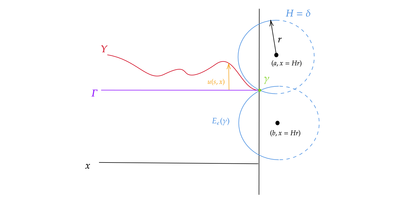
Figure 4: Picture of barrier and envelope argument

Represent $HS^{n}(R,\delta R)$ graphically over the boundary cylinder $\Gamma_{S^{n-1}}=\partial HS^{n}(R,\delta R)\times\mathbb{R}^{+}$ as

$$HS^{n}(R,\delta R)=\exp_{\overline{g}}(v(s,x)N^{n-1}(s))$$

where $\overline{N}^{n-1}(s)$ is a normal to $\partial HS^{n}(R,\delta R)\subseteq\mathbb{R}^{n}=\partial\mathbb{H}^{n+1}$. In these coordinates we have

$$v(s,x) =\sqrt{R^{2}-(x+\delta R)^{2}}-R\sqrt{1-\delta^{2}}$$

$$=v^{\prime}(0)x+O(x^{2})$$

$$=-\frac{\delta}{R^{2}(1-\delta^{2})^{3/2}}x+O(x^{2})$$

and such a construction holds for any $\delta>0$. We can repeat this construction about any $p\in\gamma$ such that $\partial HS^{n}(R,\delta R)$ lies tangent to $\gamma$ for $R=R(p)$ sufficiently small. Now consider the envelope

$$E=\partial\left(\bigcup_{p}HS^{n}(R(p),\delta R(p),p)\right)$$

$E$ is now a barrier for $Y$. Let $u(s,x)=u^{i}(s,x)\overline{N}_{i}(s,x)$. The maximum principle for $m$-mean convex submanifolds (cf. [20], [29]) then gives that about any $p$,

$$|u^{i}(s,x)| \leq|v(s,x)|$$

$$\leq C\delta x$$

where $C=C(p)$. In particular at $x=\delta$, we get

$$|u^{i}(s,\delta)|\leq C\delta^{2}$$

Noting that $\gamma$ is compact and repeating this construction for all $\delta>0$ sufficiently small, we have

$$|u^{i}(s,x)|\leq Cx^{2}$$

for all $x$ sufficiently small, and some $C$ uniform in $p\in\gamma$.

3.4.2 $M$ general PE manifold

We outline the argument as follows:

• Find $\epsilon_{0}$ sufficiently small so that when we expand

  $$g =\frac{dx^{2}+k(s,x)}{x^{2}}$$

  $$k(s,x) =k_{0}(s)+R$$

  $$||R|| \leq Cx^{2}$$ (18)

  for all $x<\epsilon_{0}$. (18) is a tensor bound in $C^{1}_{\overline{g}}$ (see §3.5)

• Let $\rho$ be the radius such that $N_{\rho}(\gamma)\subseteq\partial M$ is embedded, i.e. the normal bundle is embedded. Let $R=\rho/2$. Consider $Z:=HS^{n}(R,\delta R)$ for $\delta<\min(\epsilon_{0},\rho/2)$ and note that by (18), we have that each of the principle curvatures satisfy

  $$\kappa_{i}(Z) =\frac{\delta}{n}+E(\epsilon)$$

  $$\implies K_{m}(Z) =\sum_{i=1}^{m}\kappa_{i}(Z)=\frac{m}{n}\delta+E(\epsilon)$$

  $$E(\epsilon) \leq K\epsilon^{2}$$

  $$\implies K_{m}(Z)\Big{|}_{x=\delta} \geq c_{0}\delta$$

  The idea being that because $k(s,x)$ is even up to order $m\geq 2$, $K_{m}(Z)$ is the same up to quadratic error. Thus, a barrier which is $m$-mean strictly convex with $M=\mathbb{H}^{n+1}$ is still $m$-mean strictly convex for $M$ a general PE manifold.

• Consider the envelope $E_{\delta,R}(\gamma)$ defined by

  $$E_{\delta,R}(\gamma):=\partial\left(\bigcup_{p\in\gamma}HS^{n}(R(p),\delta R(p),p)\right)$$

  where $HS^{n}(R,\delta R,p)$ denotes the above construction based at a point $p\in\gamma$. The same $m$-mean convex maximum principle tells us that $E_{\delta,R}(\gamma)$ is a barrier for $Y$

• Let $v(s,x)$ be the graphical height function for the envelope over its boundary cylinder. As before,

  $$v(s,x) =-\frac{\delta}{R^{2}(1-\delta^{2})^{3/2}}x+O(x^{2})$$

  Then we have by the barrier arguments that

  $$|u^{i}(s,x)|\leq C\frac{\delta}{R^{2}}x$$

  Choosing $x=\delta$ (recalling that $R$ independent of $\delta$), we have

  $$|u^{i}(s,\delta)|\leq C\delta^{2}$$

  for $C$ independent of $\delta$ and $p\in\gamma$. Repeat for all $\delta>0$ sufficiently small to get

  $$\exists\delta_{0}\;\;\text{ s.t. }\;\;\forall x<\delta_{0},\qquad|u^{i}(s,x)|\leq Cx^{2}$$

3.5 Showing $v\in x^{2}\bigcap_{k}C_{0}^{k,\alpha}$

In this section, we demonstrate that $u\in x^{2}\bigcap_{k}C_{0}^{k,\alpha}$ i.e. $u$ is smooth and $u^{i}=x^{2}f^{i}$ for some $\{f^{i}\}$ such that

$$\forall j,i,\beta\quad\exists\quad C_{j\beta}^{i}<\infty\quad\text{ s.t. }\quad||(x\partial_{x})^{j}(x\partial_{s_{a}})^{\beta}f^{i}||_{C^{0,\alpha}_{0}}\leq C_{j\alpha}^{i}$$

for $j$, $\alpha$ arbitrary. Here, $C_{0}^{k,\alpha}$ is the Hölder space of functions in terms of the edge operators, $\{x\partial_{x},x\partial_{s_{a}}\}$, and

$$||f||_{C^{k,\alpha}_{0}}:=\sum_{j+|\beta|\leq k}||(x\partial_{x})^{j}(x\partial_{s_{a}})^{\beta}f^{i}||_{0,\alpha,0}$$

where $||\cdot||_{0,\alpha,0}$ denotes the geometric Hölder norm on $U$ given by

$$||f||_{0,\alpha,0}=\sup_{(s,x)\in U}|f(s,x)|+\sup_{(s,x)\neq(\tilde{s},\tilde{x})\in U}\frac{|f(s,x)-f(\tilde{s},\tilde{x})|(x+\tilde{x})^{\alpha}}{(|x-\tilde{x}|^{\alpha}+||s-\tilde{s}||_{\overline{g}}^{\alpha})}$$

where $(s,x)$ are fermi coordinates and $||s-\tilde{s}||_{\overline{g}}$ denotes the distance with respect to the compactified metric. We use $C^{k,\alpha}$ to denote the standard Hölder space with respect to the Euclidean metric. Finally, for any metric space, $(M,g)$, we denote

$$||f||_{C^{0,\alpha}_{g}}:=\sup_{p\neq q}\frac{|f(p)-f(q)|}{||p-q||_{g}^{\alpha}}$$

3.5.1 Showing $u\in C^{1,\alpha}_{0}$

Let $p_{0}=(s,z,x)=(s_{0},u(s_{0},x_{0}),x_{0})$, with $x_{0}$ sufficiently small. We consider rescaled minimal graphs (see figure 5) by changing coordinates

$$F_{0}:(s,x,z)\mapsto(\sigma,\xi,\eta):=\left(\frac{s-s_{0}}{x_{0}},\frac{x}{x_{0}},\frac{z-u(s_{0},x_{0})}{x_{0}}\right)$$

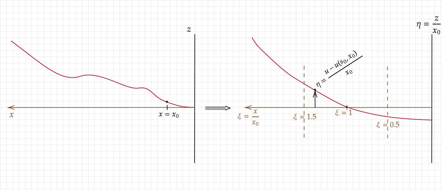
Figure 5: Visualization of rescaling with $u=u(\sigma x_{0}+s_{0},x_{0}\xi)$

Pulling back the metric by this diffeomorphism, we have

$$F_{0}^{*}(g) =F_{0}^{*}\left(\frac{dx^{2}+k(s,x,z)}{x^{2}}\right)$$

$$=\frac{d\xi^{2}+x_{0}^{2}k(x_{0}\sigma+s_{0},x_{0}\xi,x_{0}\eta+u(s_{0},x_{0}))}{\xi^{2}}$$

We expand

$$k(s,x,z) =k_{ab}(s,x,z)ds^{a}ds^{b}+k_{ai}(s,x,z)ds^{a}dz^{i}+k_{ij}(s,x,z)dz^{i}dz^{j}$$

$$x_{0}^{2}k(x_{j}\sigma+s_{0},x_{0}\xi,x_{0}\eta+u(s_{0},x_{0})) =k_{ab}(x_{0}\sigma+s_{0},x_{0}\xi,x_{0}\eta+u(s_{0},x_{0}))d\sigma^{a}d\sigma^{b}$$

$$+k_{ai}(x_{0}\sigma+s_{0},x_{0}\xi,x_{0}\eta+u(s_{0},x_{0}))d\sigma^{a}d\eta^{i}$$

$$+k_{ij}(x_{0}\sigma+s_{0},x_{0}\xi,x_{0}\eta+u(s_{0},x_{0}))d\eta^{i}d\eta^{j}$$

So that for values of $||\sigma||\leq 1$, $\frac{1}{2}\leq\xi\leq\frac{3}{2}$, $||\eta||<\frac{1}{2}$, and $x_{0}<\epsilon$, we have

$$F_{0}^{*}(g) =\frac{d\xi^{2}+k(s_{0},0,0)}{\xi^{2}}+O(x_{0})$$

here, we’ve used that $x_{0}<\epsilon$ and $|z|\leq\frac{1}{2}x_{0}$, which allows for the above expansion. In particular, we note that

$$\xi^{2}F_{0}^{*}(g) =x_{0}^{-2}F_{0}^{*}(\overline{g})$$

$$=d\xi^{2}+k(s_{0},0,0)+O(x_{0})$$

$$=d\xi^{2}+d\sigma_{1}^{2}+\dots+d\sigma_{m-1}^{2}+O(x_{0})$$

The minimal surface then becomes

$$Y_{0} :=F_{0}(Y)$$

$$(s,x,u(s,x))\mapsto(\sigma,\xi,\eta) =\left(\frac{s-s_{0}}{x_{0}},\frac{x}{x_{0}},\frac{u(x_{0}\sigma+s_{0},x_{0}\xi)-u(s_{0},x_{0})}{x_{0}}\right)$$

$$=\left(\frac{s-s_{0}}{x_{0}},\frac{x}{x_{0}},O(x_{0})\right)$$

since $\xi$ and $\eta$ are bounded. Recall the statement of Allard’s regularity theorem:

Theorem (Allard).

Suppose we have a varifold $V=v(Y^{m},\theta)\subseteq\mathbb{R}^{n+1}$, $U$ an open set in $\mathbb{R}^{n+1}$, $\eta>0$, $\rho_{0}>0$, and $p>0$, such that for all $a\in\text{spt}||V||$ and $B_{\rho}(a)\subseteq U$ with $\rho<\rho_{0}$, we have

$$1 \leq\theta\qquad\mu\;\text{a.e.}$$

$$\omega_{m}^{-1}\rho^{-m}||V||(B_{\rho}(a)) \leq 1+\eta$$

$$\left(\rho^{p-m}\int_{B_{\rho}(a)}|H|^{p}\right)^{1/p} \leq\eta$$

where $H$ is the generalized mean curvature of the varifold and $p>n$. Then up to a linear isometry of $\mathbb{R}^{n+1}$, $V$ is given graphically by $F=(F^{1},\dots,F^{n+1-m})$ on with

$$\rho^{-1}\sup|F|+\sup|DF|+\rho^{1-m/p}\sup_{a\neq b}\frac{|DF(a)-DF(b)|}{|a-b|^{1-m/p}}\leq C\eta^{1/(2m+2)}$$

with $C=C(m,n,p)$

Remark  Allard Regularity is truly a euclidean theorem, so in order to apply it, we must compute mean curvature and mass density with respect to the euclidean metric on the $(\sigma,\xi,\eta)$ coordinates, which we denote as

$$g_{euc}=d\sigma_{1}^{2}+\dots+d\sigma_{m-1}^{2}+d\xi^{2}+d\eta_{1}^{2}+\dots+d\eta_{n+1-m}^{2}$$

We verify the three conditions:

• $\theta\geq 1$ due to $Y$ being graphical

• By our assumption (13)

  $$\forall\delta>0,\qquad\exists x^{*}>0,\qquad\text{ s.t. }\qquad \forall x_{0}<x^{*}$$

  $$\omega_{m}^{-1}\rho^{-m}||V_{Y_{0},x_{0}^{-2}F_{0}^{*}(\overline{g})}||(B_{\rho}(a)) \leq 1+\delta$$

  But we’ve seen that

  $$x_{0}^{-2}F_{0}^{*}(\overline{g})=g_{euc}+O(x_{0})$$

  in $(s,x,z)$ coordinates. Thus

  $$\omega_{m}^{-1}\rho^{-m}||V_{Y_{0},g_{euc}}||(B_{\rho}(a)) \leq\omega_{m}^{-1}\rho^{-m}||V_{Y_{0},x_{0}^{-2}F_{0}^{*}(\overline{g}_{0})}||(B_{\rho}(a))+O(x_{0})$$

  $$\leq 1+\delta$$

  for $x_{0}$ (and hence $x^{*}$) sufficiently small

• We note that

  $$H_{Y_{0},euc} =H_{Y_{0},x_{0}^{-2}F_{0}^{*}(\overline{g})}+O(x_{0})$$

  $$=H_{Y_{0},\xi^{2}F_{0}^{*}(g)}+O(x_{0})$$

  $$=\frac{1}{\xi}\left[H_{Y_{0},F_{0}^{*}(g)}-m\Pi^{NY_{0}}\nabla(\ln(\xi))+O(x_{0})\right]$$

  $$=\frac{1}{\xi}\left[-m\Pi^{NY_{0}}\nabla(\ln(\xi))+O(x_{0})\right]$$

  $$\implies|H_{Y_{0},euc}| \leq C\frac{1}{\xi^{2}}$$

  $$\leq\tilde{C}$$

  having applied the formula for (generalized) mean curvature under a conformal change of metric. Here we noted that $H_{Y_{0},F_{0}^{*}(g)}=0+O(x_{0})$ and $\xi$ is bounded. Also $\Pi^{NY_{0}}$ denotes the projection onto the normal bundle of $Y_{0}$ with respect to $F_{0}^{*}(g)$. Thus $H_{Y_{0},euc}$ is bounded, in this rescaled graphical representation. This tells us that any $p$

  $$\left(\rho^{p-m}\int_{B_{\rho}(a)}|H|^{p}\right)^{1/p} \leq\left(\rho^{p-m}\rho^{m}C^{p}\right)^{1/p}$$

  $$\leq C\rho$$

  so choosing $\rho=\delta/C$ gives the desired bound.

Thus, Allard applies and we get the existence of a function

$$W=(W^{1},\dots,W^{n+1-m})\in C^{1,\alpha}$$

for $\alpha=1-m/p>0$ with the above bounds. Of course, we already have a graphical description of $Y_{0}$. Letting

$$u_{0}(\sigma,\xi):=\frac{u(x_{0}\sigma+s_{0},x_{0}\xi)-u(s_{0},x_{0})}{x_{0}}$$

Then, up to an isometry (of euclidean space), $q$, we have $W_{0}=q\circ u_{0}$ and we get the same $C^{1,\alpha}$ bounds for $u_{0}$. Note that we applied Allard with respect to $(\sigma,\xi)$ coordinates. This gives

$$||u_{0}(\sigma,\xi)||_{C^{1,\alpha}(\sigma,\xi)}\leq\delta$$

but because we’re working with $\frac{1}{2}\leq\xi\leq\frac{3}{2}$, the norm computed with $(\sigma,\xi)$ is comparable to the $C^{1,\alpha}_{0}$ and

$$||u_{0}(s,x)||_{C^{1,\alpha}_{0}}\leq\delta$$

In our ball corresponding to $\frac{1}{2}\leq\xi\leq\frac{3}{2}$.

3.5.2 Revamped Schauder Bootstrapping

From the previous section, we have a graphical representation of $Y_{0}$ in Fermi coordinates. We now consider the metric induced on $Y_{0}$ as a submanifold of $M^{n+1}$. Dropping the $0$ subindex for brevity, we use the previous sections to write the metric under the $F_{0}$ diffeomorphism as

$$\overline{h}=Id+M(\nabla u)$$

where all of the entries of $M$ can be as small as needed by choosing $\delta$ appropriately in our $C^{1,\alpha}$ bounds from §3.5.1. Therefore

$$\overline{h}^{-1}=Id-M+M^{2}+\dots=Id-M+O(\delta^{2})$$

Let $H(u)$ denote the mean curavture of the surface given by the graph of $u$ in the $(\sigma,\xi,\eta)$ coordinates. Recall the minimal surface system from Graham and Witten [12], adapted to $(\sigma,\xi,\eta)$. Here, an $a$ subindex denotes $\sigma_{a}$, $\xi$ denotes $\xi$, and $i$ denotes $\eta^{i}$:

$$0=\xi H(u)^{k} =\xi\left[\xi\partial_{\xi}-m+\frac{1}{2}{\xi}L_{\xi}\right]\left[\overline{h}^{\xi\xi}\overline{g}_{ik}u^{i}_{\xi}+\overline{h}^{a\xi}(\overline{g}_{ak}+\overline{g}_{ik}u^{i}_{a})\right]$$ (19)

$$+\xi^{2}\left[\partial_{b}+\frac{1}{2}L_{b}\right]\left[\overline{h}^{\xi b}\overline{g}_{ik}u^{i}_{\xi}+\overline{h}^{ab}(\overline{g}_{ak}+\overline{g}_{ik}u^{i}_{a})\right]$$

$$-\frac{1}{2}x^{2}\overline{h}^{ab}\left[\overline{g}_{ab,k}+2\overline{g}_{ai,k}u^{i}_{b}+\overline{g}_{ij,k}u^{i}_{a}u^{j}_{b}\right]$$

$$-\xi^{2}\overline{h}^{a\xi}[\overline{g}_{ai,k}u^{i}_{\xi}+\overline{g}_{ij,k}u^{i}_{a}u^{j}_{\xi}]$$

$$-\frac{1}{2}\xi^{2}\overline{h}^{\xi\xi}[\overline{g}_{ij,k}u^{i}_{\xi}u^{b}_{\xi}]$$

for $L=\log(\det\overline{h})$. Note that we have multipled by $\xi$ in order to make this a $0$ order differential equation (i.e. can be written in terms of edge operators $(\xi\nabla_{\sigma_{a}})$ and $(\xi\partial_{\xi})$). Ultimately, we want to write this as a quasilinear system of PDEs where

$$0=a_{\alpha\beta i}^{k}(\sigma,\xi)(\xi\partial_{y^{\alpha}})(\xi\partial_{y^{\beta}})(u^{i})+g(\xi\nabla u,\xi,\sigma)$$

where $\{y_{\alpha}\}$ denote any of $\{\sigma_{a},x\}$, $g$ is some smooth function, and $\{a_{\alpha\beta i}^{k}\}$ are uniformly elliptic. In particular, we want to show that

$$a_{\alpha\beta i}^{k}=\delta_{\alpha\beta}\delta_{i}^{k}+O(\delta)$$

for $\frac{1}{2}\leq\xi\leq\frac{3}{2}$ We break these down as follows, heavily referencing §13.2

• For the leading order term

  $$\xi(\xi\partial_{\xi})\left[\overline{h}^{\xi\xi}\overline{g}_{ik}u^{i}_{\xi}+\overline{h}^{a\xi}(\overline{g}_{ak}+\overline{g}_{ik}u^{i}_{a})\right]$$

  we see that based on the asymptotics of $\overline{h}^{\alpha\beta}$ and $\overline{g}_{ik}\Big{|}_{z=u}$ that the only contribution to ellipticity comes from

  $$i=k,\qquad\overline{h}^{\xi\xi}\overline{g}_{kk}\xi(\xi\partial_{\xi})u^{k}_{\xi} =[\xi^{2}+O(\delta)]u^{k}_{\xi\xi}+O(\delta)$$

  $$=[(\xi\partial_{\xi})^{2}-(\xi\partial_{\xi})+O(\delta)]u^{k}+O(\delta)$$

  i.e. we can write

  $$\xi(\xi\partial_{\xi})\left[\overline{h}^{\xi\xi}\overline{g}_{ik}u^{i}_{\xi}+\overline{h}^{a\xi}(\overline{g}_{ak}+\overline{g}_{ik}u^{i}_{a})\right] =(\xi\partial_{\xi})^{2}u^{k}+L_{1}u+R_{1}$$

  where $L_{1}$ is a second order parity preserving differential operator (cf. (10)) with $O(\delta)$ symbol and $\mathcal{F}(R_{1})=1$.

• For the term:

  $$-\xi m\left[\overline{h}^{\xi\xi}\overline{g}_{ik}u^{i}_{\xi}+\overline{h}^{a\xi}(\overline{g}_{ak}+\overline{g}_{ik}u^{i}_{a})\right]$$

  we note that there’s only dependence on $\xi\nabla u$ so we can ignore it for the sake of establishing ellipticity in the leading second order terms

• $L=\log(\det\overline{h})$ so that

  $$\partial_{\xi}L=\frac{\partial_{\xi}\det\overline{h}}{\det\overline{h}}$$

  we know that

  $$\det\overline{h}=1+f(\{\overline{h}_{\alpha\beta}\})$$

  where $f$ is some smooth function. We have from the appendix, equation 32, adapted to these coordinates:

  $$\overline{h}_{ab} =\overline{g}_{ab}+u_{b}^{j}\overline{g}_{aj}+u^{j}\Gamma_{bj}^{\sigma}\overline{g}_{a\sigma}$$

  $$+u_{a}^{i}\overline{g}_{ib}+u_{a}^{i}u_{b}^{j}\overline{g}_{ij}+u_{a}^{i}u^{j}\Gamma_{bi}^{\sigma}\overline{g}_{\sigma j}$$

  $$+u^{i}\Gamma_{ai}^{\mu}\overline{g}_{\mu b}+u^{i}u_{b}^{j}\Gamma_{ai}^{\mu}\overline{g}_{\mu j}+u^{i}u^{j}\Gamma_{ai}^{\mu}\Gamma_{bj}^{\sigma}\overline{g}_{\mu\sigma}$$

  $$\overline{h}_{a\xi} =u_{\xi}^{j}\overline{g}_{aj}+u^{j}\Gamma_{\xi j}^{\sigma}\overline{g}_{a\sigma}$$

  $$+u_{a}^{i}u_{\xi}^{j}\overline{g}_{ij}+u_{a}^{i}u^{j}\Gamma_{\xi i}^{\sigma}\overline{g}_{\sigma j}$$

  $$+u^{i}\Gamma_{ai}^{\mu}\overline{g}_{\mu\xi}+u^{i}u_{\xi}^{j}\Gamma_{ai}^{\mu}\overline{g}_{\mu j}+u^{i}u^{j}\Gamma_{ai}^{\mu}\Gamma_{\xi j}^{\sigma}\overline{g}_{\mu\sigma}$$

  $$\overline{h}_{\xi\xi} =1+u^{j}\Gamma_{\xi j}^{\xi}+u_{\xi}^{i}u_{\xi}^{j}\overline{g}_{ij}$$

  $$+u_{\xi}^{i}u^{j}\Gamma_{\xi j}^{\mu}\overline{g}_{i\mu}+u^{i}u_{\xi}^{j}\Gamma_{\xi i}^{\tau}\overline{g}_{\tau j}+u^{i}u^{j}\Gamma_{\xi i}^{\tau}\Gamma_{\xi j}^{\mu}$$

  all evaluated at $\eta=u$. If we compute

  $$\xi\partial_{\xi}(\det\overline{h})=Df\cdot(\{\xi\partial_{\xi}\overline{h}_{ab},\xi\partial_{\xi}\overline{h}_{a\xi},\xi\partial_{\xi}\overline{h}_{\xi\xi}\})$$

  and use the gradient bound

  $$||u(\sigma,\xi)||_{C^{1,\alpha}(\sigma,\xi)}\leq\delta$$

  we’ll see that there are no contributions to ellipticity and we can write

  $$\xi\partial_{\xi}L=L_{2}u+R_{2}$$

  where $L_{2}$ is a second order parity preserving differential operator with $o(1)$ symbol and $\mathcal{F}(R_{2})=1$.

• On the second line, we can expand

  $$\xi^{2}\partial_{\sigma_{b}}\left[\overline{h}^{\xi b}\overline{g}_{ik}u^{i}_{\xi}+\overline{h}^{ab}(\overline{g}_{ak}+\overline{g}_{ik}u^{i}_{a})\right]$$

  Clearly the only contribution to ellipticity comes from

  $$\overline{h}^{ab}\overline{g}_{ik}\xi^{2}\partial_{\sigma_{b}}(u_{a}^{i})$$

  when $i=k$. Thus we can write the above as

  $$\xi^{2}\partial_{s_{b}}\left[\overline{h}^{\xi b}\overline{g}_{ik}u^{i}_{\xi}+\overline{h}^{ab}(\overline{g}_{ak}+\overline{g}_{ik}u^{i}_{a})\right] =\delta^{ab}\delta_{i}^{k}(\xi\partial_{\sigma_{a}})(\xi\partial_{\sigma_{b}})u+L_{3}u+R_{3}$$

  where $L_{3}$ is again a parity preserving second order differential operator with $O(\delta)$ symbol and $\mathcal{F}(R_{3})=1$.

• The last 3 lines of the minimal surface equation are irrelevant for establishing ellipticity because they only involve one derivative on $u$

With this, we have that

$$0 =\xi H(u)^{k}$$

$$=a_{\alpha\beta i}^{k}(\xi,\sigma)(\xi\partial_{y_{\alpha}})(\xi\partial_{y_{\beta}})u^{i}+g(\xi\nabla u,\xi,\sigma)$$

where for $\frac{1}{2}\leq\xi\leq\frac{3}{2}$,

$$a_{\alpha\beta i}^{k}=\delta_{\alpha\beta}\delta_{i}^{k}+O(\delta)$$

and we can write

$$0 =\xi^{2}\partial_{\alpha}^{2}u^{k}+K_{i}^{\alpha\beta}(\nabla u,\xi,\sigma)\partial_{\alpha}\partial_{\beta}u^{i}+b_{i}^{\gamma}(\nabla u,\xi,\sigma)(\partial_{\gamma}u^{i})+F(\nabla u,\xi,\sigma)u+G(\nabla u,\xi,\sigma)$$

$$=[\delta_{\alpha\beta}\xi^{2}+K_{i}^{\alpha\beta}]\partial_{\alpha}\partial_{\beta}u^{i}+b_{i}^{\gamma}\partial_{\gamma}u^{i}+Fu+G$$

for some coefficients $K_{i}^{\alpha\beta}=O(\delta)$ and $b_{i}^{\gamma}=O(\delta)$ for each $k$. Here, $\{K_{i}^{\alpha\beta}\}$ and $\{b_{i}^{\gamma}\}$ are both $O(\delta)$ in $C^{\alpha}_{(\sigma,\xi)}$ because of their dependence of $\nabla u$ and the fact that $||u(\sigma,\xi)||_{C^{1,\alpha}}=\delta$. Moreover, $F=G=0$ because the minimal surface system is a divergence system, i.e. it can be written as a collection of equations each of the form

$$\text{div}\left(\vec{A}_{\alpha}\cdot\frac{\partial u^{i}}{\partial y_{\alpha}}\right)=0$$

We now apply Schauder estimates using that the functions $K_{i}^{\alpha\beta}(\nabla u,\xi,\sigma)$, $B_{i}^{\gamma}(\nabla u,\xi,\sigma)$, and $F(u,\xi,\sigma)$ are all in $C^{\alpha}$

$$||u(\xi,\sigma)||_{C^{2,\alpha}} \leq\mathrm{T}\left(||u||_{C^{0,\alpha}}+||G||_{C^{0,\alpha}}\right)=\mathrm{T}\left(||u||_{C^{0,\alpha}}\right)$$

See [8] section 5 or [27] for the proof of Schauder estimates in the systems case. We can further improve this:

$$||u||_{C^{0,\alpha}}\leq||u||_{C^{1,\alpha}}\leq\tilde{T}||u||_{C^{0}}=O(x_{j})$$

having used first order Schauder estimates in the second inequality. We now iterate this argument to get bounds on higher derivatives in terms of the rescaled variables, $(\sigma,\xi)$. This ensures smoothness away from $x=0$ as well as bounds on higher derivatives in terms of constants independent of $j$. Note that in the above, we’ve been working with standard Hölder norms in the $(\sigma,\xi)$ variables and the $C^{k,\alpha}$ Hölder norms. But again, because $1/2\leq\xi\leq 3/2$ we get comparable bounds for the $C^{k,\alpha}_{0}$ norms for the $(s,x)$ coordinates.

We proved that for $u_{0}$, there exists a $\delta$ (and hence $x_{0}$) sufficiently small so that

$$u_{0}(\sigma,\xi)\in x_{0}\bigcap_{k}C_{0}^{k,\alpha}\qquad\forall k\geq 0$$

Undoing the definition of $u_{0}(\sigma,\xi)$ in terms of the original function $u$, we get

$$u(x_{0}\sigma+s_{0},x_{0}\xi)=x_{0}u_{0}(\sigma,\xi)+u(s_{0},x_{0})$$

Thus we actually have that $u$ is regular at $x=x_{0}$ in a neighborhood of radius $x_{0}$. This construction holds for all $x_{0}$ sufficiently small, so we conclude

$$u\in x^{2}\bigcap_{k}C_{0}^{k,\alpha}\qquad\forall k\geq 0$$

i.e.

$$u=x^{2}f,\qquad\forall j,\beta,\quad\exists\;C_{j\beta}^{i}<\infty\quad\text{ s.t. }\quad||(x\partial_{x})^{j}(x\partial_{s_{a}})^{\beta}f^{i}||_{C^{0,\alpha}}\leq C_{j\beta}^{i}$$

3.6 Parametrix Argument

Having shown that

$$u\in x^{2}\bigcap_{k}C_{0}^{k,\alpha}$$

we now want to show that

$$u\in x^{2}\bigcap_{k}C^{k,\alpha}_{b}$$

i.e. for $u=x^{2}f$, we have

$$\forall j,|\beta|\;\in\mathbb{Z}^{+},\qquad\exists\;\tilde{C}_{j\beta}^{i}\;\;\text{ s.t. }\;||(x\partial_{x})^{j}(\partial_{s_{a}})^{\beta}f^{i}||_{C_{0}^{0,\alpha}}\leq\tilde{C}_{j\beta}^{i}$$

(note that we use $\partial_{s_{a}}$, not $(x\partial_{s_{a}})$!). To show this, we briefly recall relevant facts from microlocal analysis and the theory of edge operators from [26]

• The space of conormal functions is

  $$\mathcal{A}:=\bigcap_{k}C^{k,\alpha}_{b}$$

• The space of polyhomogeneous function is

  $$\mathcal{A}_{phg}:=\{u(s,x)\;|\;u(s,x)\sim\sum_{\text{Re}(z_{j})\to\infty}\sum_{t=0}^{N_{j}}x^{z_{j}}\log(x)^{t}a_{j,t}(s)\;\;\text{ s.t. }\;\;N_{j}<\infty,\qquad a_{j,t}\in C^{\infty}\}$$

  where for $m>|\beta|>0$

  $$\forall\epsilon>0,\qquad\Big{|}D^{\beta}\left(u(s,x)-\sum_{\text{Re}(z_{j})<m}\sum_{t=0}^{N_{j}}x^{z_{j}}\log(x)^{t}a_{j,t}(s)\right)\Big{|}=O(x^{m-|\beta|-\epsilon})$$

  i.e. the remainder and its derivatives (in $x$ and $s_{a}$ variables) decay at a faster rate. In practice, we’ll be dealing with $z_{j}$ real, positive, and integer valued.

• We denote the space of edge operators, $V_{e}$, and the space of $b$-operators, $V_{b}$ as

  $$V_{e} =\text{span}_{C^{\infty}(\mathcal{U})}\{(x\partial_{x}),(x\partial_{s_{a}})\}$$

  $$V_{b} =\text{span}_{C^{\infty}(\mathcal{U})}\{(x\partial_{x}),\partial_{s_{b}}\}$$

  for $\mathcal{U}$ the neighborhood of $\Gamma$ as defined in §2.6

• The weighted Hölder space of orders $\ell\in\mathbb{N}$, $\alpha\in(0,1)$, and $\delta\in\mathbb{R}$ are

  $$x^{\delta}\Lambda^{\ell,\alpha}_{0}:=\{u=x^{\delta}v\;\text{ s.t. }\;V_{1}\cdots V_{j}v\in\Lambda^{0,\alpha}_{0},\qquad\forall V_{i}\in V_{e},\;\;j\leq\ell\}$$

  where $\Lambda^{0,\alpha}_{0}=C^{0,\alpha}$ is the geometric Hölder space with norm

  $$||f||_{0,\alpha,0}=\sup|f|+\sup_{(s,x)\neq(\tilde{s},\tilde{x})}\frac{(x+\tilde{x})^{\alpha}|f(s,x)-f(\tilde{s},\tilde{x})|}{|x-\tilde{x}|^{\alpha}+||s-\tilde{s}||_{\overline{g}}^{\alpha}}$$

  We also define

  $$x^{\delta}\Lambda^{\ell,\alpha,m}_{0}=\{u=x^{\delta}v\;\text{ s.t. }\;(V_{1}\cdots V_{j})(\tilde{V}_{1}\cdots\tilde{V}_{k})v\in\Lambda^{0,\alpha}_{0},\qquad V_{i}\in V_{e},\;\tilde{V}_{i}\in V_{b},\qquad\;\;j\leq\ell,\;k\leq m\}$$

• $\Psi^{m,\mathcal{E}}$ denotes pseudodifferential operators in the small calculus. $\Psi^{m,\mathcal{E}}_{0}$ denotes the large calculus. $\Psi^{m,\mathcal{E}}_{b}$ denotes the analogous calculus but with respect to the $b$-operators

• For $L\in\Psi^{m,\mathcal{E}}_{0}$ an elliptic pseudodifferential operator, a parametrix, $G\in\Psi^{-m,\mathcal{E}}_{0}$, exists such that

  $$LG =I-R_{1}$$

  $$GL =I-R_{2}$$

  where $I$ is the identity and $R_{1},R_{2}\in\Psi^{-\infty,\mathcal{E}}$ are “residual” operators. Here, $m$ is the order of the principal symbol of $L$. Roughly speaking, $R_{i}$ sends functions of any regularity into polyhomogeneous functions.

We also recall a few relevant propositions from [26] adopted for our case of the index set $\mathcal{E}=\{0,m+1\}$

• (Proposition $3.27$) For $A\in\Psi^{m,\mathcal{E}}_{0}$, suppose $\ell\geq m$ and $\delta>-1$, then

  $$A:x^{\delta}\Lambda^{\ell,\alpha}_{0}\to x^{\delta}\Lambda^{\ell-m,\alpha}_{0}$$

• (Proposition $3.28$) For $f\in\mathcal{A}_{phg}$, $A\in\Psi_{0}^{m,\mathcal{E}}$, we have $Af\in\mathcal{A}_{phg}$

• (Proposition $3.30$) For $v\in V_{b}$, $A\in\Psi_{0}^{m,\mathcal{E}}$, we have $[v,A]\in\Psi_{e}^{m,\mathcal{E}}$

Remark  Hereafter, we use $O(x^{k})$ to denote a remainder term which lies in $x^{k}\mathcal{A}$, and $o(x^{k})$ to a remainder term, $f$, such that $\lim_{x\to 0}x^{-k}f=0$ with convergence in $\mathcal{A}$.

We now prove that $u\in x^{2}\mathcal{A}$. We argue as follows: for $\overline{N}_{i}=\partial_{z_{i}}$ a basis for $N(\Gamma)$ ($z_{i}$ are Fermi coordinates for the normal bundle), we have $u=u^{i}\overline{N}_{i}$ and

$$0 =H(u)=H(0)+L_{0}(u)+Q_{0}(u)$$

$$\implies L_{0}(u)^{i} =-H(0)^{i}-Q_{0}(u)^{i}$$

where $L_{0}=J_{\Gamma}$ is the Jacobi operator on $\Gamma\subseteq M$ and also the linearization of the mean curvature functional about $u=0$. $Q_{0}$ is the quadratic remainder from the linearization and depends on $\{x\nabla u,x,s\}$, which are parameters in the coefficients for our elliptic system of equations which we’ve bounded in the previous section. Here $Q_{0}(u)=O(x^{4})$ because $u=O(x^{2})$, and the superscript denotes the $\overline{N}_{i}$th component. We have

$$L_{0}(u)=\Delta_{\Gamma}(u)+\tilde{A}_{\Gamma}(u)-(m+E(x))u$$

Here, $\Delta_{\Gamma}$ is the Laplacian on $\Gamma$ on the normal bundle computed with respect to the $(\xi,\sigma)$ variables, $\tilde{A}$ is the Simons operator, a $0$th order operator that is $O(x^{2})$ (see §5), and $E(x)=O(x^{2})$ is an error term coming from the computation of $\text{tr}_{\Gamma}[R_{M}(\cdot,u)\cdot]$ as in the standard Jacobi operator. Let $G$ be a parametrix for this operator

$$GL =I-R$$

$$GL(u)^{i} =u^{i}-(Ru)^{i}$$

$$=-(GH(0))^{i}+(GQ)^{i}$$

$$\implies u^{i} =-(GH(0))^{i}+(GQ)^{i}+(Ru)^{i}$$

$$=GQ^{i}+F^{i}$$

where $Ru$ is a residual term. One can compute $H(0)=x^{2}H_{\gamma}+O(x^{4})$ analytic in $x$ and $s$. By Propositions $3.27$ and $3.28$, we have that $GH(0)$ is $O(x^{2})$ and polyhomogeneous. Moreover, because $R$ is residual, we have that $Ru$ is polyhomogeneous. Finally by $3.27$, we know that $GQ=O(x^{4})$. With this, we can write

$$u^{i}+(GH(0))^{i}-(GQ)^{i}=(Ru)^{i}$$

and note that the left hand side is $O(x^{2})$, so $(Ru)^{i}$ must be both $O(x^{2})$. This tells us that $F^{i}:=-(GH(0))^{i}+(Ru)^{i}$ is $O(x^{2})$ and polyhomogeneous. We now differentiate this equation to get

$$\partial_{s_{a}}u^{i}=\partial_{s_{a}}F^{i}+G(x^{-1}(x\partial_{s_{a}})Q)+[\partial_{s_{a}},G]Q$$

Again, $\partial_{s_{a}}F^{i}$ is $O(x^{2})$ by polyhomogeneity. From our initial estimates, we have that $x^{-1}(x\partial_{s_{a}})Q=O(x^{3})$, and by Proposition $3.27$, $G(x^{-1}(x\partial_{s_{a}})Q)\in x^{3}\cap_{k}C^{k,\alpha}_{0}$. Similarly, by $3.30$ and $3.27$, we have that $[\partial_{s_{a}},G]Q=x^{4}\bigcap_{k}C^{k,\alpha}_{0}$ because $Q=O(x^{4})$. This shows that

$$u\in\bigcap_{k}x^{2}\Lambda^{k,\alpha,1}_{0}$$

We now proceed by induction. Assume that

$$u\in x^{2}\bigcap_{k}x^{2}\Lambda^{k,\alpha,j}_{0}$$

For $\alpha$ a multi-index of order $j+1$, we write

$$\partial_{s_{a_{1}}}\cdots\partial_{s_{a_{j+1}}}u=\partial_{s}^{\alpha}u=\partial_{s}^{\alpha}(GQ^{i}+F^{i})=\partial_{s}^{\alpha}(GQ^{i})+\partial_{s}^{\alpha}(F^{i})$$

we automatically have that $\partial_{s}^{\alpha}F^{i}\in x^{2}\Lambda_{0}^{k,\alpha,j}$ for any $k$ and $j$ since $F^{i}$ is polyhomogenous. For the first term, we write

$$\partial_{s}^{\alpha} =\partial_{s_{a}}\partial_{s}^{\beta},\qquad|\beta|=j$$

$$\partial_{s}^{\beta}(GQ^{i}) =\sum_{|\gamma|+|\delta|=j}c_{\gamma}[\partial_{s_{\gamma_{1}}},\cdots,[\partial_{s_{\gamma_{j}}},G]]\partial_{s}^{\delta}Q^{i}$$

where $c_{\gamma}$ is some integer valued coefficient reflecting the combinatorics of how many commutator terms we get. By induction and the chain rule, we know that $\partial_{s}^{\delta}Q^{i}$ is $O(x^{4})$ for all $\delta$. By repeated application of Proposition $3.30$, we know that the nested commutator term lies in $\Psi^{-2,\mathcal{E}}_{e}$. Then by Proposition $3.27$ and $3.28$, we can conclude that

$$c_{\gamma}[\partial_{s_{\gamma_{1}}},\cdots,[\partial_{s_{\gamma_{j}}},G]]\partial_{s}^{\delta}Q^{i}\in x^{4}\bigcap_{k}C^{k,\alpha}_{0}$$

so that

$$\partial_{s_{a}}\left(c_{\gamma}[\partial_{s_{\gamma_{1}}},\cdots,[\partial_{s_{\gamma_{j}}},G]]\partial_{s}^{\delta}Q^{i}\right)=x^{-1}(x\partial_{s_{a}})\left(c_{\gamma}[\partial_{s_{\gamma_{1}}},\cdots,[\partial_{s_{\gamma_{j}}},G]]\partial_{s}^{\delta}Q^{i}\right)\in x^{3}\bigcap_{k}C^{k,\alpha}_{0}$$

adding the $F^{i}$ term we have

$$u\in x^{2}\bigcap_{k}\Lambda_{0}^{k,\alpha,j+1}$$

This completes the induction and we get

$$u\in x^{2}\bigcap_{k,j}\Lambda_{0}^{k,\alpha,j}=x^{2}\bigcap_{k}C^{k,\alpha}_{b}=x^{2}\mathcal{A}$$

3.7 Expanding Mean Curvature Functional

We now compute the linearization of the mean curvature functional, $H$, on graphical submanifolds of the form $\{\vec{u}(s,x)\}$ from before. We first linearize about $u_{0}=0$:

$$H(u)=H(0)+L(u)+Q(u)$$

so that in (19), we set $0=z^{i}=p^{i}_{\alpha}$ when evaluating $\overline{h}^{\alpha\beta}$ as abstract functions of $(x,\{z^{i}\},\{p^{i}_{\alpha}\})$ to be set equal to $(x,\{u^{i}\},\{u^{i}_{\alpha}\})$. Here, $Q(u)$ is an expression that’s at least quadratic in the components of $\{u,x\nabla u\}$ and depends smoothly on $s$. Because $u\in x^{2}\mathcal{A}$, we have $Q(u)\in x^{4}\mathcal{A}$. Note that $H(0)$ is the mean curvature of the graph corresponding to $\vec{u}(s,x)=0$, which is just $\Gamma=\mathbb{R}^{+}\times\gamma$. A short computation gives

$$H(0) =H_{\{u=0\}}$$

$$=[x^{2}H_{\gamma}^{i}+R^{i}]\overline{N}_{i}$$

$$R^{i} =O(x^{4})$$

$$\mathcal{F}(R^{i}) =1$$

where $H_{\gamma}^{i}$ are the components of the mean curvature of the boundary submanifold, computed with the compactified metric restricted to the boundary. In particular, we note that

$$R^{i}=\begin{cases}R^{i}_{4}x^{4}+\dots+R^{i}_{n+2}x^{n+2}+R^{i}x^{n+2}\log(x)+O(x^{n+3}\log(x))&n\text{ even }\\ R^{i}_{4}x^{4}+\dots+R^{i}_{n+2}x^{n+2}+O(x^{n+3})&n\text{ odd}\end{cases}$$ (20)

With this, we note that

$$L =(\text{Jacobi operator evaluated at $\{u=0\}$ graph})$$

$$=\Delta_{\{u=0\}}+\tilde{A}_{\{u=0\}}+\text{Tr}[R_{M}(\cdot,\_)\cdot]=\Delta_{\Gamma}+\tilde{A}_{\Gamma}+\text{Tr}[R_{M}(\cdot,\_)\cdot]$$

for $\tilde{A}$ the Simons operator. Here, let

$$\begin{gathered}u=u^{i}\overline{N}_{i}=\hat{u}^{i}\hat{N}_{i}\\ \hat{u}_{i}=x^{-1}u^{i},\qquad\hat{N}_{i}:=x\overline{N}_{i}\end{gathered}$$

Note that $g(\hat{N}_{i},\hat{N}_{i})=1+O(x^{2})$ on $\Gamma$. This choice of notation is so that geometric operators with respect to $g$ act more naturally on $\hat{u}^{i}$ as opposed to $u^{i}$ due to the choice of normalization. Following the work of [11] (corollary 2.8) along with §13.4 and §13.5, we can write

$$L(u)=[(x\partial_{x})^{2}-(m-1)(x\partial_{x})-m](\hat{u}^{i})(\hat{N}_{i})+E(x^{-1}u)^{i}(x\hat{N}_{i})$$

where $E$ is an error term that is at most second order in $V_{b}$ operators and has $O(x^{2})$ coefficients and analogously to (20) can only have $x^{k}\log(x)$ terms at $k\geq n+2$. Thus $E(u)^{i}=O(x^{3})$. Via §13.5, we see that $\tilde{A}_{\{u=0\}}(u)=f_{i}\hat{N}_{i}$ where $f_{i}=O(x^{3})$. With this, we begin our iteration at

$$H(u) =0=H(0)+L(u)+Q(u)$$

$$=x^{2}H_{\gamma}+[(x\partial_{x})^{2}-(m-1)(x\partial_{x})-m](\hat{u}^{i})\hat{N}_{i}+O(x^{4})$$

3.8 Iteration Argument

Having extracted the linear term and shown that the remainder is $O(x^{2})$, we write

$$L(u) =-H(0)-Q(u)$$

$$=-xH_{\gamma}^{i}\hat{N}_{i}-Q(u)-R_{0}$$

$$=[-xH_{\gamma}^{i}+O(x^{3})]\hat{N}_{i}$$

Hence

$$((x\partial_{x})^{2}-(m-1)(x\partial_{x})-m)(\hat{u}^{i})\hat{N}_{i} =-xH_{\gamma}^{i}\hat{N}_{i}+[-Q(u)+O(x^{4})]\hat{N}_{i}$$

$$\implies((x\partial_{x})^{2}-(m-1)(x\partial_{x})-m)(\hat{u}^{i}) =-xH_{\gamma}^{i}+O(x^{4})$$

We now factor and integrate

$$((x\partial_{x})^{2}-(m-1)(x\partial_{x})-m)(\hat{u}^{i}) =(x\partial_{x}+1)(x\partial_{x}-m)(\hat{u}^{i})$$

$$\implies(x\partial_{x}-m)\hat{u}^{i} =-\frac{1}{2}H_{\gamma}^{i}x+O(x^{3})$$

having used an integrating factor of $x^{-2}$, integrated from $x_{0}=0\to x$, and noted that $\hat{u}^{i}\in x\mathcal{A}$ to rule out the constant term. We multiply by the integrating factor $x^{-m-1}$ and do the same

$$x^{-m}\hat{u}^{i}_{x}-mx^{-m-1}\hat{u}^{i} =-\frac{1}{2}H_{\gamma}^{i}x^{-m}+O(x^{2-m})$$

$$\frac{d}{dx}(x^{-m}\hat{u}^{i}) =-\frac{1}{2}H_{\gamma}^{i}x^{-m}+O(x^{2-m})$$

$$\implies x^{-m}\hat{u}^{i} =-\frac{1}{2(1-m)}H_{\gamma}^{i}x^{-m+1}+O(x^{3-m})+K$$

$$\hat{u}^{i} =\frac{1}{2(m-1)}H_{\gamma}^{i}x+O(x^{3})$$

where we include $K$ when we integrate from some $x_{0}>0$ to $x$. This is valid when $m\geq 3$ since we absorb $Kx^{m}$ into $O(x^{3})$. Converting back to $u^{i}=x\hat{u}^{i}$, this process gives an explicit formula for $u_{2}^{i}(s)$:

Lemma.

The minimal submanifold, $Y^{m}$, can be described as a graph over $\Gamma=\partial Y\times[0,\epsilon)$ via

$$Y\cap\{0\leq x<\epsilon\}=\{\overline{\exp}_{(\gamma(s),x)}(u(s,x))\quad|\quad 0\leq x<\epsilon,\qquad\gamma(s)\in\gamma\}$$

where $u(s,x)=u^{i}(s,x)\overline{N}_{i}=u^{i}(s,x)\partial_{z_{i}}$ and

$$\boxed{u^{i}(s,x)=\frac{1}{2(m-1)}H_{\gamma}^{i}x^{2}+O(x^{3})}$$

Where $\partial_{z_{i}}$ is a Fermi coordinate basis for the normal bundle with respect to the compactified metric and $H_{\gamma}$ is the mean curvature of $\gamma\subseteq\partial M$, and $m\geq 2$.

We now want to iterate this argument to get an even expansion up to $m$, with a potential log term when $m$ is odd.

Proof of Theorem 3.1:
We first do $m$ even. Assume the inductive hypothesis of

$$\hat{u}^{i}=p_{2k-1}^{i}(x)+f^{i}(x),\qquad\qquad f^{i}(x)=o(x^{2k-1})\qquad 2k<m$$

where $p_{2k-1}^{i}$ is an odd polynomial in $x$ of order $2k-1$ with coefficient depending smoothly on $s$ and $f^{i}\in\mathcal{A}$. Further assume

$$H(p_{2k-1}^{i}\hat{N}_{i})=O(x^{2k+1})=[a_{2k+1}^{i}x^{2k+1}+o(x^{2k+1})]\hat{N}_{i}$$

We have established the base case, $k=0$ with $p_{0}^{i}=0$ and $a_{2}^{i}=\frac{1}{2(m-1)}H_{\gamma}^{i}$. For higher values of $k$, we can expand

$$H([p_{2k-1}^{i}+f^{i}]\hat{N}_{i})=H((p_{2k-1}^{i}\hat{N}_{i})+L_{p_{2k-1}^{i}\hat{N}_{i}}(f^{i}\hat{N}_{i})+Q_{p_{2k-1}\hat{N}_{i}}(f^{i}\hat{N}_{i})$$

Abbreviate $L_{2k-1}:=L_{p_{2k-1}^{i}\hat{N}_{i}}$. This is the linearized operator (i.e. Jacobi Operator) corresponding to the graph of $\{u=p_{2k-1}^{i}\hat{N}_{i}\}$. Then using the fact that $p_{2k-1}^{i}=O(x)$ produces a graphical asymptotically hyperbolic manifold with odd coefficients up to at least order $x^{2}$, we have as before

$$L_{2k-1} =I_{L_{2k-1}}+T_{L_{2k-1}}$$

$$I_{L_{2k-1}} =[(x\partial_{x})^{2}-(m-1)(x\partial_{x})-m]$$

$$T_{L_{2k-1}} :x^{k}\mathcal{A}\to x^{k+2}\mathcal{A}$$

$$\implies L_{2k-1}(f^{i}\hat{N}_{i}) =[(x\partial_{x})^{2}-(m-1)(x\partial_{x})-m](f^{i})\hat{N}_{i}+o(x^{2k+1})$$

where “$I_{L_{2k-1}}$” stands for the indicial operator of the linearization at $p_{2k-1}$ and $T_{L_{2k-1}}$ is the remainder. Finally, $Q_{2k-1}(f^{i}\hat{N}_{i}):=Q_{p_{2k-1}^{i}\hat{N}_{i}}(f^{i}\hat{N}_{i})$ will be at least $x^{2}$ times the order of $f^{i}$ and hence of order $o(x^{2k+1})$. Thus

$$0 =H(\hat{u}^{i}\hat{N}_{i})=H([p_{2k-1}^{i}+f^{i}]\hat{N}_{i})$$

$$=H(p_{2k-1}^{i}\hat{N}_{i})+L_{2k-1}(f^{i}\hat{N}_{i})+Q_{2k-1}(f^{i}\hat{N}_{i})$$

$$=a_{2k+1}^{i}x^{2k+1}\hat{N}_{i}+[(x\partial_{x}-m)(x\partial_{x}+1)f^{i}]\hat{N}_{i}+o(x^{2k+1})$$

Rearranging and matching vector components, we get

$$(x\partial_{x}+1)(x\partial_{x}-m)f^{i}=-a_{2k+1}^{i}x^{2k+1}+o(x^{2k+1})$$

as before, we perform an integrating factor for $(x\partial_{x}+1)$ first and then $(x\partial_{x}-m)$

$$x^{-m-1}(x\partial_{x}-m)f^{i} =-\frac{a_{2k+1}^{i}}{2k+1}x^{2k-m}+o(x^{2k-m})$$

$$\partial_{x}(x^{-m}f^{i}) =-\frac{a_{2k+1}^{i}}{2k+1}x^{2k-m}+o(x^{2k-m})$$ (21)

$$f^{i} =-\frac{a_{2k+1}^{i}}{(2k-m+1)(2k+1)}x^{2k+1}+Kx^{m}+o(x^{2k+1})$$

we see that the denominators are never $0$ when $m$ is even. Note that $K$ is the constant from evaluating $x^{-m}f$ at some point $x=x_{0}$ small but non-zero. This shows that we can continue to induct and get the next even term in our expansion as long as $2k<m$.

When $2k=m$, the above process shows that $f^{i}=K^{\prime}x^{m+1}+O(x^{m+1})$ and we can continue the expansion but the expansion is no longer even. Converting back to $u^{i}=x\hat{u}^{i}$, we have

$$m\text{ even }\implies u^{i} =\frac{1}{2(m-1)}H_{\gamma}^{i}x^{2}+\dots+u_{m}^{i}x^{m}+u_{m+1}^{i}x^{m+1}+O(x^{m+2})$$

i.e. $\mathcal{F}(u^{i})=1$. In particular our remark about (20) shows that when $m=n$ even, there is no $x^{n}\log(x)$ term because $x^{k}\log(x)$ error terms occur for $k\geq n+1$ in the iteration.

When $m$ is odd, most of the proof remains the same. However, when $2k=m-1$, we see that 21 becomes

$$\partial_{x}(x^{-m}f^{i}) =-\frac{a_{m}^{i}}{m}x^{-1}+o(x^{-1})$$

$$x^{-m}f^{i} =K-\frac{a_{m}^{i}}{m}\log(x)+o(\log(x))$$

$$f^{i} =Kx^{m}-\frac{a_{m}^{i}}{m}x^{m}\log(x)+o(x^{m}\log(x))$$

so a log term appears in this case. After setting

$$p_{2k+1}^{i}=p_{2k-1}^{i}-\frac{a_{m}^{i}}{m}x^{m}\log(x)+Kx^{m}$$

we can continue the iteration without $\log$ terms but we lose evenness of the expansion. Converting back to $u^{i}$, we conclude

$$m\text{ odd }\implies u^{i} =\frac{1}{2(m-1)}H_{\gamma}^{i}x^{2}+\dots+u_{m+1}^{i}x^{m+1}+U^{i}x^{m+1}\log(x)+u_{m+2}x^{m+2}+O(x^{m+3})$$

which is again, the statement of $\mathcal{F}(u^{i})=1$. ∎

As a consequence of these computations we get the following result about the induced metric on $Y$

Corollary 3.1.2.

The induced metric on $Y$ satisfies for

$$\mathcal{F}(\overline{h}_{\alpha\beta}) =(-1)^{\sigma(\alpha)+\sigma(\beta)}$$

$$\overline{h}_{xx} =1+O(x^{2})$$

$$\overline{h}_{xa} =O(x^{3})$$

$$\overline{h}_{ab} =\delta_{ab}+O(x^{2})$$

where $\sigma(\alpha)$ is as in equation (17).

Remark  We can take the analysis further for $m=n$ even:

Corollary 3.1.3.

For $m=n$ even,

$$[\overline{h}_{ab}]^{\log,n+1} =0$$

$$[\overline{h}_{xx}]^{\log,n} =0$$

$$[\overline{h}_{xx}]^{\log,n+1} =0$$

$$[\sqrt{\det\overline{h}}]^{\log,n+1} =0$$

This follows from the explicit formula for $v_{a}$ and $v_{x}$ in (32) and holds for all coefficients $K$ in the $Kx^{n}\log(x)$ term of (3). Note that $\overline{h}_{ab}$ and $\sqrt{\det\overline{h}}$ may have an $x^{n}\log(x)$ term.

4 Parity of Second Fundamental Form

In this section we aim to prove the following theorem:

Theorem 4.1.

Suppose that $Y^{m}\subseteq M^{n+1}$ minimal with $\overline{h}=\overline{g}\Big{|}_{TY}$ even up to order $x^{m}$. Let $p\in Y$ and $\overline{A}:\text{Sym}^{2}(TY)\to N(Y)$ denote the second fundamental form, and let $\{w_{i}(s,x)\}$ be the frame for the normal bundle described in §13.3. Define

$$T_{\gamma\delta i;\alpha_{1}\cdots\alpha_{p}}:=\overline{g}\left((\overline{\nabla}_{v_{\alpha_{1}}}\cdots\overline{\nabla}_{v_{\alpha_{p}}}\overline{A})(v_{\gamma},v_{\delta}),w_{i}\right)$$

where $\alpha_{i}$ can take on any of the indices $\{s_{1},\dots,s_{m-1},x\}$. Let $q$ denote the number of “$x$”s among the indices $\{\gamma,\delta,\alpha_{1},\dots,\alpha_{p}\}$, then we have

$$\forall i,\qquad\mathcal{F}(T_{\gamma\delta i;\alpha_{1}\cdots\alpha_{p}})=(-1)^{q}$$

We notate the following

$$\overline{A}_{\alpha\beta} =\overline{g}(\overline{\nabla}_{F_{\alpha}}F_{\beta})$$ (22)

$$\tilde{\overline{\Gamma}}_{\sigma\tau\omega} :=g(\overline{\nabla}_{v_{\sigma}}v_{\tau},v_{\omega})$$ (23)

$$\overline{h}_{\alpha\beta}(t) :=\overline{g}(F_{\alpha},F_{\beta})$$ (24)

where $\overline{\nabla}$ is the connection with respect to $\overline{g}$. We also define $\overline{A}_{\alpha\beta i}$, the components of $\overline{A}_{\alpha\beta}$, and $\overline{A}_{\alpha\beta}^{i}$ and $\tilde{\overline{\Gamma}}_{\sigma\tau}^{\omega}$ by raising the tensors appropriately. Finally, we let the indices $\{\sigma,\tau,\omega,\mu\}$ denote any vector in the basis for $TM=TY\oplus NY$, i.e. $v_{\sigma},v_{\tau},v_{\omega}\in\{v_{s_{a}},v_{x},\nu_{i}\}$ and similarly with $F_{\alpha}\in\{F_{a},F_{x}\}\subseteq TY_{t}$. Note that

$$\overline{A}_{\alpha\beta}=\tilde{\overline{\Gamma}}_{\alpha\beta}^{j}w_{j}$$

for $\alpha$, $\beta$ denoting $v_{\alpha},v_{\beta}\in TY$.

4.0.1 Lemmas for theorem 4.1

We start by writing the tangent basis for $Y$ in fermi decomposition

$$v_{a} =G_{*}(\partial_{s_{a}})=\partial_{s_{a}}+u_{a}^{i}\partial_{z_{i}}+u[\overline{\Gamma}_{ai}^{b}\partial_{s_{b}}+\overline{\Gamma}_{ai}^{j}\partial_{j}+\overline{\Gamma}_{ai}^{x}\partial_{x}]$$

$$v_{x} =G_{*}(\partial_{x})=\partial_{x}+u_{x}^{i}\partial_{z_{i}}+u[\overline{\Gamma}_{xi}^{a}\partial_{s_{a}}+\overline{\Gamma}_{xi}^{j}\partial_{z_{i}}]$$

Similarly, recall the parity of the coefficients for our normal frame: (cf. section §13.2 and lemma 13.3)

$$w_{i} =c^{a}_{i}(s,x)\partial_{s_{a}}+c^{x}_{i}(s,x)\partial_{x}+c^{j}_{i}(s,x)\partial_{z_{j}}$$

$$\mathcal{F}(c^{a}_{i}) =1$$

$$\mathcal{F}(c^{x}_{i}) =-1$$

$$\mathcal{F}(c^{j}_{i}) =1$$

Let $\overline{\Gamma}_{\sigma\tau\omega}$ denote the christoffel symbols in the basis of $\{\partial_{s_{a}},\partial_{x},\partial_{z_{i}}\}$, with respect to $\overline{g}$, in a tubular neighborhood of $\Gamma=\gamma\times\mathbb{R}^{+}$, parameterized by $(s,x,z)$.

Lemma 4.2.

We have

$$\forall p\in Y,\qquad\mathcal{F}\left(\overline{\Gamma}_{\sigma\tau\omega}\Big{|}_{p\in Y}\right)=(-1)^{q}$$ (25)

where $q$ is the number of indices among $\sigma$, $\tau$, $\omega$ that are equal to $x$

Proof: First note that via the fermi coordinate decomposition

$$\overline{\Gamma}_{xxb}=\overline{\Gamma}_{xxi}=0$$

And also

$$\overline{\Gamma}_{\alpha i\beta}=\overline{g}(\overline{\nabla}_{\partial_{y_{\alpha}}}\partial_{z_{i}},\partial_{y_{\beta}})=-\overline{g}(\partial_{z_{i}},\overline{\nabla}_{\partial_{y_{\alpha}}}\partial_{y_{\beta}})=-\overline{\Gamma}_{\alpha\beta i}$$

and so it suffices to consider $\overline{\Gamma}_{\cdot\cdot i}$, $\overline{\Gamma}_{axb}$, $\overline{\Gamma}_{abx}$, and $\overline{\Gamma}_{abc}$. The proof of the result comes from the splitting of the ambient metric under Graham-Lee Normal form in a tubular neighborhood of the boundary (i.e. on $\partial M\times[0,\epsilon)$):

$$\overline{g}=dx^{2}+k(x,s,z)$$

Here, $k(x,s,z)$ is a $2$-tensor such that $k(x,s,z)(\partial_{x},\cdot)\equiv 0$. Moreover $k(s,x,z)$ expands as

$$\text{$n+1$ even}\implies k(s,x) =k_{0}+x^{2}k_{2}+\cdots+k_{n-1}x^{n-1}+k_{n}x^{n}+k_{n+1}x^{n+1}+O(x^{n+2})$$

$$\text{$n+1$ odd}\implies k(s,x) =k_{0}+x^{2}k_{2}+\cdots+k_{n}x^{n}+Kx^{n}\log(x)+k_{n+1}x^{n+1}+O(x^{n+2})$$

where each $k_{i}=k_{i}(s,z)$ is a $2$-tensor. $k_{i}(s,z)$ can also be expanded up to order $z^{m}$ in $z$ since $z=(z^{1},\dots,z^{n+1-m})$ is a system of fermi coordinates and $\gamma$ is $C^{m+1,\alpha}$ embedded in $\partial M$. so we can expand

$$k_{i}(s,z) =k_{i,0}(s)+k_{i,1}(s)z+\dots+k_{i,p}(s)z^{m}+O(z^{m+1})$$

for any $z$. Evaluating this on $Y$ (i.e. $z=u(s,x)$), we see that $k(s,x,u(s,x))$ is a tensor that is even in $x$ up to order $x^{m+1}$. With this and the Koszul formula, one can directly show the parity statements in (25) hold in a tubular neighborhood of $\gamma\times[0,\epsilon)\subseteq\partial M\times[0,\epsilon)$. ∎

We now extend this to compute the Christoffel’s in the basis of $\{v_{a},v_{x},w_{i}\}$: Let $\tilde{\overline{\Gamma}}$ be as in (23), i.e.

$$\tilde{\overline{\Gamma}}_{\alpha\beta\gamma} :=g(\overline{\nabla}_{v_{\alpha}}v_{\beta},v_{\gamma}),\qquad \tilde{\overline{\Gamma}}_{\alpha\beta i}:=g(\overline{\nabla}_{v_{\alpha}}v_{\beta},w_{i})$$

$$\tilde{\overline{\Gamma}}_{\alpha i\beta} :=g(\overline{\nabla}_{v_{\alpha}}w_{i},v_{\beta}),\qquad \tilde{\overline{\Gamma}}_{\alpha ij}:=g(\overline{\nabla}_{v_{\alpha}}w_{i},w_{j})$$

$$\tilde{\overline{\Gamma}}_{i\alpha\beta} :=g(\overline{\nabla}_{w_{i}}v_{\alpha},v_{\beta}),\qquad \tilde{\overline{\Gamma}}_{i\alpha j}:=g(\overline{\nabla}_{w_{i}}v_{\alpha},w_{j})$$

$$\tilde{\overline{\Gamma}}_{ij\alpha} :=g(\overline{\nabla}_{w_{i}}w_{j},v_{\alpha}),\qquad \tilde{\overline{\Gamma}}_{ijk}:=g(\overline{\nabla}_{w_{i}}w_{j},w_{k})$$

and $\tilde{\overline{\Gamma}}^{\omega}_{\sigma\tau}$ the raised versions of these christoffels by the induced metric on $Y$.

Lemma 4.3.

For $\tilde{\overline{\Gamma}}_{\sigma\mu\omega}$ as above evaluated on $Y$, we have that

$$\forall p\in Y,\qquad\mathcal{F}\left(\tilde{\overline{\Gamma}}_{\sigma\mu\omega}\Big{|}_{p\in Y}\right)=(-1)^{q}$$

where $q$ the number of $x$’s among the indices $\sigma$, $\mu$, $\omega$.

Proof: Again, this boils down to recording parity of the coefficients of $\{v_{a},v_{x},w_{i}\}$ in the basis of $\partial_{s_{a}},\partial_{x},\partial_{z_{i}}$. We’ll compute the first christoffel and leave the remainder to the reader

$$\overline{\nabla}_{v_{a}}v_{b} =\overline{\nabla}_{\partial_{s_{a}}}(\partial_{s_{b}}+u_{b}^{j}\partial_{z_{j}}+u\overline{\Gamma}_{bj}^{\sigma}\partial_{y_{\sigma}})$$

$$+u_{a}^{i}\overline{\nabla}_{\partial_{z_{i}}}(\partial_{s_{b}}+u_{b}^{j}\partial_{z_{j}}+u\overline{\Gamma}_{bj}^{\sigma}\partial_{y_{\sigma}})$$

$$+u\overline{\Gamma}_{ai}^{\sigma}\overline{\nabla}_{\partial_{y_{\sigma}}}(\partial_{s_{b}}+u_{b}^{j}\partial_{z_{j}}+u\overline{\Gamma}_{bj}^{\sigma}\partial_{y_{\sigma}})$$

$$=A_{1}+A_{2}+A_{3}$$

We have

$$A_{1} =\overline{\Gamma}_{ab}^{\omega}\partial_{y_{\omega}}+u_{ab}^{j}\partial_{z_{j}}+u_{b}^{j}\overline{\Gamma}_{bj}^{\sigma}\partial_{y_{\sigma}}$$

$$+u\overline{\Gamma}_{bj,a}^{\sigma}\partial_{y_{\sigma}}+u\overline{\Gamma}_{bj}^{\sigma}\overline{\Gamma}_{a\sigma}^{\omega}\partial_{y_{\omega}}$$

$$A_{2} =u_{a}^{i}\Big{[}\overline{\Gamma}_{ib}^{\omega}\partial_{y_{\omega}}+u_{b}^{j}\overline{\Gamma}_{ij}^{\omega}\partial_{y_{\omega}}$$

$$+u\overline{\Gamma}_{bj,i}^{\sigma}\partial_{y_{\sigma}}+u\overline{\Gamma}_{bj}^{\sigma}\overline{\Gamma}_{i\sigma}^{\omega}\partial_{y_{\omega}}\Big{]}$$

$$A_{3} =u\Gamma_{ai}^{\sigma}\Big{[}\overline{\Gamma}_{\sigma b}^{\mu}\partial_{y_{\mu}}+u_{b,\sigma}^{i}\partial_{z_{j}}+u_{b}^{j}\overline{\Gamma}_{\sigma j}^{\omega}\partial_{y_{\omega}}$$

$$+u_{\sigma}\overline{\Gamma}_{nj}^{\mu}\partial_{y_{\mu}}+u\overline{\Gamma}_{bj,\sigma}^{\mu}\partial_{y_{\mu}}+u\Gamma_{bj}^{\mu}\Gamma_{\sigma\mu}^{\tau}\partial_{y_{\tau}}\Big{]}$$

One can now compute using lemma 4.2 that

$$\mathcal{F}(g(A_{i},\partial_{s_{c}})) =1$$

$$\mathcal{F}(g(A_{i},\partial_{z_{j}})) =1\implies\mathcal{F}(u^{j}g(A_{i},\partial_{z_{j}}))=1$$

$$\mathcal{F}(g(A_{i},\partial_{y_{\mu}})) =(-1)^{\sigma(\mu)}\implies\mathcal{F}(u\Gamma_{ci}^{\mu}g(A_{i},\partial_{y_{\mu}}))=1$$

$$\implies\mathcal{F}(g(A_{i},v_{c})) =1$$

which verifies that $(\Gamma_{abc})=1$. The remaining symbols proceed similarly. ∎

Finally, we establish a short lemma about the metric in the basis of $\{v_{a},v_{x},w_{i}\}$:

$$\overline{W}_{\alpha\beta} =\overline{g}(v_{\alpha},v_{\beta})$$

$$\overline{W}_{\alpha i} =\overline{g}(v_{\alpha},w_{i})$$

$$\overline{W}_{ij} =\overline{g}(w_{i},w_{j})$$

and $\overline{W}^{\gamma\delta}$ is defined as the inverse.

Lemma 4.4.

For $\overline{W}$ as above, we have

$$\mathcal{F}(\overline{W}_{\gamma\delta})=\mathcal{F}(\overline{W}^{\gamma\delta})=(-1)^{p}$$

where $p$ is the number of $x$’s among $\gamma$ and $\delta$

Proof: This comes from taking the decomposition of the normal, $\{w_{i}\}$ and tangent frames, $\{v_{\alpha},v_{x}\}$ for $NY$, $TY$, as given in section §13.2 and section §13.3, and then noting that parity is preserved under inversion. ∎

As a result of this, we define

$$\overline{\Gamma}_{\sigma\mu}^{\omega}:=\overline{W}^{\omega\nu}\overline{\Gamma}_{\sigma\mu\omega}$$

and conclude

Corollary 4.4.1.

$$\mathcal{F}(\overline{\Gamma}_{\sigma\mu}^{\omega})=(-1)^{p}$$

where $p$ the number of $x$’s among the indices $\sigma$, $\mu$, $\omega$

4.1 Proof of theorem 4.1

We prove theorem 4.1

Theorem.

Suppose that $Y^{m}\subseteq M^{n+1}$ minimal with $\overline{h}=\overline{g}\Big{|}_{TY}$ even up to order $x^{m}$. Let $p\in Y$ and $\overline{A}:\text{Sym}^{2}(TY)\to N(Y)$ denote the second fundamental form, and let $\{w_{i}(s,x)\}$ be the frame for the normal bundle described above. Define

$$T_{\gamma\delta i;\alpha_{1}\cdots\alpha_{p}}:=\overline{g}\left((\overline{\nabla}_{v_{\alpha_{1}}}\cdots\overline{\nabla}_{v_{\alpha_{p}}}\overline{A})(v_{\gamma},v_{\delta}),w_{i}\right)$$

where $\alpha_{i}$ can take on any of the indices $\{s_{a},x\}$. Let $q$ denote the number of “$x$”s among the indices $\{\gamma,\delta,\alpha_{1},\dots,\alpha_{p}\}$, then we have

$$\forall i,\qquad\mathcal{F}(T_{\gamma\delta i;\alpha_{1}\cdots\alpha_{p}})=(-1)^{q}$$

Proof: The base case is an application lemma 4.3 as

$$\overline{A}_{\alpha\beta i} =\tilde{\overline{\Gamma}}_{\alpha\beta i}$$

$$\implies\mathcal{F}(\overline{A}_{\alpha\beta i}) =\mathcal{F}(\tilde{\overline{\Gamma}}_{\alpha\beta i})=(-1)^{\sigma(\alpha)+\sigma(\beta)}$$

Now from here, we prove the theorem by induction for

$$g((\overline{\nabla}_{v_{\alpha_{1}}}\cdots\overline{\nabla}_{v_{\alpha_{n}}}\overline{A})(v_{\gamma},v_{\delta}),w_{i})$$

where $\{v_{\delta},v_{\gamma},v_{\alpha_{i}}\}\in\{v_{\alpha},v_{x}\}$. Assume the parity statement holds for $n-1$. We compute

$$(\overline{\nabla}_{v_{\alpha_{1}}}\cdots\overline{\nabla}_{v_{\alpha_{n}}}\overline{A})(v_{\gamma},v_{\delta}) =\overline{\nabla}_{v_{\alpha_{1}}}^{\perp}[(\overline{\nabla}_{v_{\alpha_{2}}}\cdots\overline{\nabla}_{v_{\alpha_{n}}}\overline{A})(v_{\gamma},v_{\delta})]$$

$$-(\overline{\nabla}_{v_{\alpha_{2}}}\cdots\overline{\nabla}_{v_{\alpha_{n}}}\overline{A})(\overline{\nabla}_{v_{\alpha_{1}}}^{\|}v_{\gamma},v_{\delta})$$

$$-(\overline{\nabla}_{v_{\alpha_{2}}}\cdots\overline{\nabla}_{v_{\alpha_{n}}}\overline{A})(v_{\gamma},\overline{\nabla}_{v_{\alpha_{1}}}^{\|}v_{\delta})$$

$$=I_{1}+I_{2}+I_{3}$$

here $\overline{\nabla}^{\|}=\overline{\nabla}^{Y}$ is the connection on $TY$ and $\overline{\nabla}^{\perp}$ is the connection on $NY$ (both using $\overline{h}$). Let $p_{n-1}$ denote the number of $x$’s among the indices $\{\alpha_{2},\dots,\alpha_{n},\gamma,\delta\}$. For any index, $\omega$, recall the $\sigma(\omega)$ notation 17. We have

$$\mathcal{F}(g(I_{1},w_{i})) =\mathcal{F}\left(\overline{g}(\overline{\nabla}_{v_{\alpha_{1}}}^{\perp}[(\overline{\nabla}_{v_{\alpha_{2}}}\cdots\overline{\nabla}_{v_{\alpha_{n}}}\overline{A})(v_{\gamma},v_{\delta})],w_{i})\right)$$

$$=\mathcal{F}\left(v_{\alpha_{1}}g((\overline{\nabla}_{v_{\alpha_{2}}}\cdots\overline{\nabla}_{v_{\alpha_{n}}}\overline{A})(v_{\gamma},v_{\delta}),w_{i})-g((\overline{\nabla}_{v_{\alpha_{2}}}\cdots\overline{\nabla}_{v_{\alpha_{n}}}\overline{A})(v_{\gamma},v_{\delta}),\overline{\nabla}_{v_{\alpha_{1}}}^{\perp}w_{i})\right)$$

By the inductive hypothesis, we have

$$\mathcal{F}\left(v_{\alpha_{1}}g((\overline{\nabla}_{v_{\alpha_{2}}}\cdots\overline{\nabla}_{v_{\alpha_{n}}}\overline{A})(v_{\gamma},v_{\delta}),w_{i})\right)=(-1)^{\sigma(\alpha_{1})+p_{n-1}}$$

And similarly

$$\overline{\nabla}_{v_{\alpha_{1}}}^{\perp}w_{i}=\tilde{\overline{\Gamma}}_{\alpha_{1}i}^{k}w_{k}$$

so that

$$\mathcal{F}(g((\overline{\nabla}_{v_{\alpha_{2}}}\cdots\overline{\nabla}_{v_{\alpha_{n}}}\overline{A})(v_{\gamma},v_{\delta}),\overline{\nabla}_{v_{\alpha_{1}}}^{\perp}w_{i})) =\mathcal{F}(\tilde{\overline{\Gamma}}_{\alpha_{1}i}^{k})\mathcal{F}(g((\overline{\nabla}_{v_{\alpha_{2}}}\cdots\overline{\nabla}_{v_{\alpha_{n}}}\overline{A})(v_{\gamma},v_{\delta}),w_{k}))$$

$$=(-1)^{\sigma(\alpha_{1})+p_{n-1}}$$

again by the inductive hypothesis and lemma 4.3. For $I_{2}$ and $I_{3}$, we have

$$I_{2} =(\overline{\nabla}_{v_{\alpha_{2}}}\cdots\overline{\nabla}_{v_{\alpha_{n}}}\overline{A})(\overline{\nabla}_{v_{\alpha_{1}}}^{\|}v_{\gamma},v_{\delta})$$

$$=\tilde{\overline{\Gamma}}_{\alpha_{1}\gamma}^{\mu}(\overline{\nabla}_{v_{\alpha_{2}}}\cdots\overline{\nabla}_{v_{\alpha_{n}}}\overline{A})(v_{\mu},v_{\delta})$$

$$\mathcal{F}(g(I_{2},w_{i})) =\mathcal{F}(\tilde{\overline{\Gamma}}_{\alpha_{1}\gamma}^{\mu})\mathcal{F}\left(g((\overline{\nabla}_{v_{\alpha_{2}}}\cdots\overline{\nabla}_{v_{\alpha_{n}}}\overline{A})(v_{\mu},v_{\delta}),w_{i})\right)$$

$$=(-1)^{\sigma(\alpha_{1})+\sigma(\mu)+\sigma(\gamma)}(-1)^{p_{n-1}+\sigma(\mu)-\sigma(\gamma)}$$

$$=(-1)^{\sigma(\alpha_{1})+p_{n-1}}$$

This follows by expanding $\overline{\nabla}_{v_{\alpha_{1}}}v_{\gamma}$ and using lemma 4.4.1. $I_{3}$ proceeds analogously. This finishes the induction. ∎

5 Asymptotics for the variational vector field

Having established an expansion for $u$, we want to show the analogous expansion for our variational vector fields $\dot{S}:=F_{*}(\partial_{t})\Big{|}_{t=0}$ and $\ddot{S}=\nabla_{F_{*}(\partial_{t})}F_{*}(\partial_{t})\Big{|}_{t=0}$. We first need to fix a frame for the normal bundle.

Lemma.

For any $p\in\gamma$ and a neighborhood $N(p)\subseteq M$, there exists a frame $\{w_{1},\dots,w_{n+1-m}\}$ for $N(Y)$ which is orthonormal on $(\gamma,\overline{g}\Big{|}_{\gamma})$ such that

$$\overline{g}(w_{i},\partial_{x})=\text{$O(x)$ and odd up to order $m-1$}$$

$$\overline{g}(w_{i},\partial_{s_{a}})=\text{$O(x^{2})$ and even up to order $m+2$}$$

$$\overline{g}(w_{i},\partial_{r_{j}})=\text{$\delta_{ij}+O(x^{2})$ and even up to order $m$}$$

Alternatively, we phrase this as

$$w_{i} =c^{a}_{i}(s,x)\partial_{s_{a}}+c^{x}_{i}(s,x)\partial_{x}+c^{j}_{i}(s,x)\partial_{z_{j}}$$

$$\mathcal{F}(x^{-2}c^{a}_{i}) =1$$

$$\mathcal{F}(c^{x}_{i}) =-1$$

$$\mathcal{F}(c^{j}_{i}) =1$$

This is done by taking a normal frame for $\gamma\subseteq\partial M$, translating it to the interior so that the frame is constant in $x$, and projecting onto $TY^{\perp}$. See (13.3) in the appendix. With this frame, we prove

Theorem 5.1.

Consider $\dot{S}=\dot{\phi}^{i}(s,x)w_{i}(s,x)$ and $\ddot{S}=\ddot{\phi}^{i}(s,x)w_{i}(s,x)$ be the first and second variational vector fields for a family of minimal submanifolds $\{Y_{t}\}_{t\geq 0}$ with $Y$ as in §2. Then

$$\mathcal{F}(\dot{\phi}^{i}) =1$$

$$\mathcal{F}(\ddot{\phi}^{i}) =1$$

Moreover, when $m=n$ even, there are no $x^{n}\log(x)$ or $x^{n+1}\log(x)$ terms.

The theorem says that in a good ($x$-dependent!) frame for the normal bundle, we have a polyhomogeneous expansion to all orders which is even up to order $m$ ($m+1$) for $m$ even (odd). The idea is that $\dot{S}$ satisfies a homogeneous Jacobi equation since $Y_{0}$ is minimal, and $\ddot{S}$ satisfies an inhomogeneous Jacobi Equation since $\{Y_{t}\}$ is a variation through minimal submanifolds. We leverage these equations to deduce a polyhomogeneous expansion of $\dot{\phi}^{i}$ and $\ddot{\phi}^{i}$ by doing the analogous PDE analysis for the minimal surfaces system as in section §3.

5.1 Jacobi Operator in full codimension

By definition, $Y_{t}:=\exp_{Y}(S_{t})$ and $\dot{S}=\partial_{t}S_{t}\Big{|}_{t=0}$. Given that $\{Y_{t}\}$ is a family of minimal submanifolds, $\dot{S}$ lies in the kernel of the Jacobi operator

$$J(X)=\Delta_{Y}^{\perp}X+\tilde{A}(X)+\text{Tr}[R_{M}(\cdot,X)\cdot]$$

Here $\Delta_{Y}^{\perp}$ denotes the laplacian on the normal bundle, $\tilde{A}(X)$ denotes the Simons’ operator on $Y$, and $\text{Tr}[R_{M}(\cdot,X)\cdot]$ is a trace of the ambient Riemann curvature tensor over $TY$. As we showed in section §3.7, we have

Proposition 1.

For $Y^{m}\subseteq M^{n+1}$ as in our setup, the Jacobi operator decomposes as

$$J(\phi^{i}w_{i})=[(x\partial_{x})^{2}-(m-1)(x\partial_{x})-m](\phi^{i})\;w_{i}+R^{i}(\{\phi^{j}\})w_{i}$$

where

$$R:x^{\delta}C^{k+2,\alpha}_{0}(Y)\to x^{\delta+2}C^{k,\alpha}_{0}(Y)$$

is an error term

In particular, if we expand $R$

$$R=\sum_{p,\beta}r_{p,\beta}(s,x)(x\partial_{x})^{p}(x\partial_{s})^{\beta}$$

for $\beta$ a multi-index, then $r_{p,\beta}=O(x^{2})$ and $\mathcal{F}(r_{p,\beta})=1$. Because we have $\dot{\phi}^{i}=O(1)$, we see that the same PDE analysis and iteration argument as in section §3.8 gives

$$\mathcal{F}(\dot{\phi}^{i})=1$$

as desired. ∎

Remark  Note that if we choose to expand $\dot{S}$ in powers of $x$, we lose parity

$$\dot{S} =\dot{S}_{0}(s)+x\dot{S}_{1}(s)+x^{2}\dot{S}_{2}(s)+\dots$$

$$\dot{S}_{i} \in T_{p}M,\qquad p\in Y$$

i.e. both even and odd terms appear! This is because $N(Y)$ “tilts” with $x$ so a priori, we have no parity of $\dot{S}$ in powers of $x$ with $x$-independent vectors, $\{\dot{S}_{k}(s)\}$.

5.2 Regularity and Parity of $\ddot{S}$

Proposition 2.

Let $\{Y_{t}\}\subseteq M^{n+1}$ be a family of minimal of $m$-dimensional minimal submanifolds. Let $Y=Y_{0}$ and $\overline{h}$ denote a compactified metric on $Y$. Then for

$$Y_{t}=\{\exp_{\overline{h},p}(S_{t}(p)\overline{\nu}(p))\;|\;p\in Y\}$$

The second variation of mean curvature is given by

$$\frac{d^{2}}{dt^{2}}H_{t}=J_{Y}^{\perp}(\ddot{S})+Q^{\perp}(\dot{S})$$

where $Q^{\perp}$ is a quadratic differential functional in $\dot{S}$ and $\mathcal{F}(Q^{\perp}(\dot{S}))=1$

The details and the verification that

$$Q^{\perp}(\dot{S}) =Q^{i}(s,x)w_{i}$$

$$\mathcal{F}(Q^{i}) =1$$

are shown in the appendix §13.10. By the same work with $\dot{S}$, this immediately gives

Theorem 5.2.

Let $\{Y_{t}\}\subseteq M^{n+1}$ be a family of minimal of $m$-dimensional minimal submanifolds. Let $Y=Y_{0}$ and $\overline{h}$ denote a compactified metric on $Y$. Then for

$$Y_{t}=\{\exp_{\overline{h},p}(S_{t}(p))\;|\;p\in Y\}$$

with $S_{t}(p)\in NY$ for all $t$ and $\{w_{i}\}$ the normal basis described in 13.3, we have

$$\ddot{S}=\frac{d^{2}}{dt^{2}}\Big{|}_{t=0}S_{t}=\ddot{S}^{i}w_{i}$$

Moreover

$$\mathcal{F}(\ddot{S}^{i})=1$$

and when $m=n$ even, there are no $x^{n}\log(x)$ or $x^{n+1}\log(x)$ terms.

Having shown that $\{u^{i}\}$, $\{\dot{\phi}^{j}\}$, and $\{\ddot{\phi}^{k}\}$ have polyhomogeneous expansions, we compute the variations of renormalized volume. Recall that we have $\{Y_{t}\}$ a one parameter family of minimal submanifolds. Intuitively

$$\frac{d}{dt}\mathcal{V}(Y_{t}) =\frac{d}{dt}\underset{z=0}{FP}\;\int_{Y_{t}}x^{z}dA_{Y_{t}}=\frac{d}{dt}\underset{z=0}{FP}\;\int_{Y}F_{t}^{*}(x)^{z}F_{t}^{*}(dA_{t})=\underset{z=0}{FP}\;\int_{Y}zx^{z-1}K(\dot{S},u)$$

$$=\underset{z=0}{FP}\;zg(z)$$

where $x:\overline{M}\to\mathbb{R}^{\geq 0}$ is a special bdf for $\overline{M}$ and $g(z)=\int_{Y}x^{z-1}K(\dot{S},u)$ for some function $K$ to be determined.

6 Mechanics of Finite Part Evaluation

When computing variations of renormalized volume, we encounter integrals of the form

$$I(z)=\int_{Y}z^{p}b(x,s)x^{z-j}dA_{Y}$$

for $b$ having a polyhomogeneous expansion in $x$ (after pulling back to $\Gamma$) and $i\geq 0$, $j\in\{0,1,2\}$. We write

$$I(z)=\left(\int_{Y\cap\{x<\delta\}}+\int_{Y\cap\{x\geq\delta\}}\right)z^{p}b(x,s)x^{z-j}dA_{Y}=I_{1}(z,\delta)+z^{p}I_{2}(z,\delta)$$

for some $1\gg\delta>0$, where we’ve pulled out the factor of $z^{p}$ in the $\{x\geq\delta\}$. As before, $I_{2}(z)$ is holomorphic because the integral is over $x\geq\delta$. In particular

$$\underset{z=0}{FP}\;z^{p}I_{2}(z,\delta)=\begin{cases}I_{2}(0,\delta)&p=0\\ 0&p\geq 1\end{cases}$$

We further assume the following expansions (after pulling back to Fermi coordinates)

$$dA_{Y} =\frac{\sqrt{\det\overline{h}}}{x^{m}}dx\wedge dA_{\gamma}$$

$$\sqrt{\det\overline{h}} =\sum_{k=0}^{m+2}\overline{q}_{j}(s)x^{k}+\tilde{Q}(s)x^{m}\log(x)+\overline{Q}(s)x^{m+1}\log(x)+O(x^{m+2}\log(x))$$

$$b(x,s) =\sum_{k=0}^{m+2}b_{j}(s)x^{k}+\tilde{B}(s)x^{m}\log(x)+B(s)x^{m+1}\log(x)+O(x^{m+2}\log(x))$$

i.e. if a $x^{d}\log(x)^{q}$ term manifests, it can occur only when $d\geq m$. This accounts for both even and odd expansion of $u(s,x)$ and $\{\overline{h}^{\alpha\beta}\}$ as in §3. $I_{1}$ expands as

$$I_{1}(z,\delta) =z^{p}\int_{0}^{\delta}\int_{\gamma}x^{z-m-j}\left[\sum_{\ell=0}^{m+2}\sum_{k+j=\ell}b_{k}\overline{q}_{j}x^{\ell}\right]dsdx$$

$$+z^{p}\int_{0}^{\delta}\int_{\gamma}x^{z-m-j}\left[(\overline{q}_{0}\tilde{B}+\tilde{Q}b_{0})x^{m}\log(x)+(b_{0}\overline{Q}+b_{1}\tilde{Q}+\overline{q}_{0}B+\overline{q}_{1}\tilde{B})x^{m+1}\log(x)\right]dsdx$$

$$+z^{p}\int_{0}^{\delta}\int_{\gamma}x^{z-m-j}\left[(b_{1}\overline{Q}+b_{2}\tilde{Q}+\overline{q}_{1}B+\tilde{B}\overline{q}_{2})x^{m+2}\log(x)\right]dsdx$$

$$+z^{p}\int_{0}^{\delta}\int_{\gamma}O(x\log(x))dsdx$$

Observe that

$$\underset{z=0}{FP}\;z^{p}\int_{0}^{\delta}\int_{\gamma}O(x\log(x))dx=\begin{cases}C(\delta)&p=0\\ 0&p\geq 1\end{cases}$$

for some finite constant $C(\delta)$. It remains to compute

$$\underset{z=0}{FP}\;I_{1}(z,\delta) =\underset{z=0}{FP}\;z^{p}\sum_{k=0}^{m+2}c_{k}\int_{0}^{\delta}x^{z+k-m-j}dx$$

$$+\underset{z=0}{FP}\;z^{p}\sum_{k=0}^{2}c_{m+k}^{*}\int_{0}^{\delta}x^{z+k-m-j}\log(x)dx$$

for

$$c_{k} =\int_{\gamma}\left[\sum_{\ell+j=k}b_{\ell}\overline{q}_{j}\right]dV_{\gamma},\qquad 0\leq k\leq m+2$$

$$c_{m}^{*} =\int_{\gamma}\left[\overline{q}_{0}\tilde{B}+\tilde{Q}b_{0}\right]dA_{\gamma}$$

$$c_{m+1}^{*} =\int_{\gamma}\left[b_{0}\overline{Q}+b_{1}\tilde{Q}+\overline{q}_{0}B+\overline{q}_{1}\tilde{B}\right]dA_{\gamma}$$

$$c_{m+2}^{*} =\int_{\gamma}\left[b_{1}\overline{Q}+b_{2}\tilde{Q}+\overline{q}_{1}B+\tilde{B}\overline{q}_{2}\right]dA_{\gamma}$$

Integrating,

$$I_{1}(z,\delta)=z^{p}\left(c_{m+j-1}\frac{\delta^{z}}{z}+c^{*}_{m+j-1}\frac{\delta^{z}((z\log(\delta)-1)}{z^{2}}+F(\delta,z)\right)$$

where $F(\delta,z)$ is holomorphic near $z=0$. In particular

$$\underset{z=0}{FP}\;z^{p}F(\delta,z) =\begin{cases}F(\delta,0)&p=0\\ 0&p\geq 1\end{cases}$$

$$\underset{z=0}{FP}\;z^{p}\frac{\delta^{z}}{z} =\begin{cases}\log(\delta)&p=0\\ 1&p=1\\ 0&p>1\end{cases}$$

$$\underset{z=0}{FP}\;z^{p}\frac{\delta^{z}(z\log(\delta)-1)}{z^{2}} =\begin{cases}\frac{\log(\delta)^{2}}{2}&p=0\\ 0&p=1\\ -1&p=2\\ 0&p\geq 3\end{cases}$$

Note that a $x^{d}\log(x)$ term in the expansion of $I_{1}$ leads to higher order poles. We summarize this work as

Lemma 6.1.

Consider integrals of the form

$$I(z)=\int_{Y}z^{p}b(x,s)x^{z-j}dA_{Y}$$

for $b$ and $dA_{Y}$ having polyhomogeneous expansions in $x$ and $p\geq 0$, $j\in\{0,1,2\}$. Moreover, assume that $x^{d}\log(x)^{q}$ terms only manifest when $d\geq m$ and $q=1$, or $d\geq m+3$. Then we have that

$$\underset{z=0}{FP}\;I(z)=\begin{cases}C(\delta)+F(\delta,0)+I_{2}(0,\delta)+c_{m+j-1}\log(\delta)+c^{*}_{m+j-1}\frac{\log(\delta)^{2}}{2}&p=0\\[4.30554pt] c_{m+j-1}&p=1\\[4.30554pt] -c^{*}_{m+j-1}&p=2\\[4.30554pt] 0&p\geq 3\end{cases}$$

for the coefficients $\{c_{k}\}$ listed above

Remark:

• This calculation illustrates the following key point: when at least one factor of $z$ appears, the finite part can be expressed as an integral over the boundary. We will refer to this process from here on as localization.

• In practice, $b(x,s)$ and $\overline{q}(x,s)$ satisfy $\mathcal{F}=1$ or $\mathcal{F}=-1$ which reduces the above

• In the future we write

  $$B=[b(x,s)]^{k,\log}$$

  to indicate the $x^{k}\log(x)$ term

• Taking $b(x,s)=1$ and $p=0$ demonstrates how to compute the renormalized volume of $Y$ via Riesz regularization

• While the result for $p=0$ seems to depend on $\delta$, one can show that by changing $\delta\to\delta^{\prime}$ and keeping track of boudary terms from the intermediate integral $\int_{x=\delta}^{\delta^{\prime}}$, the result is independent of $\delta$. This is done out for $b(x,s)=1$ in §13.6

7 Renormalized Volume for $Y\subseteq M^{n+1}$

Let $x_{Y}$ be a special bdf on $(Y,h)$ considered as its own asymptotically hyperbolic manifold with metric even to high order. In this section, we prove the following:

Theorem 7.1.

Let $Y^{m}\subseteq M^{n+1}$ minimal, satisfying the conditions §3 and $x_{Y}$ a special bdf on $Y$. Let $x$ a special bdf on $M$, inducing the same conformal infinity on $Y$. We have that

$$\underset{z=0}{FP}\;\int_{Y}x_{Y}^{z}dA_{Y}=\begin{cases}\underset{z=0}{FP}\;\int_{Y}x^{z}dA_{Y}&\text{ m even }\\[8.61108pt] \int_{\gamma}p(s)dA_{\gamma}(s)+\underset{z=0}{FP}\;\int_{Y}x^{z}dA_{Y}&\text{ m odd }\end{cases}$$

where $p(s)$ is some function on the boundary determined by $u_{2}(s)=\frac{1}{2(m-1)}H_{\gamma}(s)$ and its derivatives.

This theorem says that for even dimensional manifolds, we can use either a special bdf on $Y$, which is labeled as $x_{Y}$, or the almost special bdf, $x$, on $M^{n+1}$. Recall that a special bdf, $x$, satisfies

$$||dx||_{\overline{g}}^{2}=\overline{g}^{xx}=1$$

where $\overline{g}=x^{2}g$. We want to find a special bdf, $x_{Y}$, for $Y$, such that

$$||dx_{Y}||_{\overline{h}}^{2}=\overline{h}^{\alpha\beta}dx_{Y}(v_{\alpha})dx_{Y}(v_{\beta})=1$$

where $\{v_{\alpha}\}$ is the pushforward of the coordinate basis for $TY$ defined in 13.2 and $\overline{h}$ is the restriction of $\overline{g}$ to $Y$. As in [1], [11] and [12], we begin with a bdf on $Y$ written as

$$x_{Y}(x)=xe^{\omega(s,x)}$$

where

$$\omega(s,x)=\sum_{k=0}^{\infty}\omega_{k}(s)x^{k}$$

such an expansion was shown in [11]. We now enforce $1=||d\log(x_{Y})||_{h}^{2}$:

$$1 =h^{\alpha\beta}e^{-2\omega}x^{-2}[e^{\omega}dx(v_{\alpha})+xe^{\omega}d\omega(v_{\alpha})][e^{\omega}dx(v_{\beta})+xe^{\omega}d\omega(v_{\beta})]$$ (26)

$$=\overline{h}^{\alpha\beta}[dx(v_{\alpha})+xd\omega(v_{\alpha})][dx(v_{\beta})+xd\omega(v_{\beta})]$$

As in [11], the above equation shows that $\omega_{1}=0$, and in general that $\omega$ has an even expansion to high order. When $m$ is even, the first non-trivial odd coefficient occurs at $x^{m+1}$, with potentially an $x^{m}\log(x)$ in the codimension $1$ case. When $m$ is odd, there may be $x^{m}\log(x)$ and $x^{m+1}\log(x)$ terms. In both cases, the first odd order term in (26) comes from the first odd order terms in the expansion of $\{\overline{h}^{\alpha\beta}\}$. To summarize:

Lemma: Let $Y^{m}\subseteq M^{n+1}$ be a minimal submanifold. There exists a bdf $x_{Y}:Y\to\mathbb{R}^{+}$ such that

$$x_{Y}(s,x)=xe^{\omega(s,x)}$$

with

$$\mathcal{F}(\omega)=1$$

We now prove theorem 7.1

7.1 Equivalence of Renormalized Volume of $Y^{n}\subseteq M^{n+1}$, $m$ even

Let $x$ be a special bdf on $M$ and $x_{Y}$ a special bdf for $Y$. We compute the following difference

$$\int_{Y}(x^{z}-x_{Y}^{z})dA_{Y} =\underset{z=0}{FP}\;\int_{Y}x^{z}(1-e^{\omega(s,x)z})dA_{Y}=\int_{Y}(z\omega+O(z^{2}))dA_{Y}$$

$$=\underset{z=0}{FP}\;\int_{Y}z\omega dA_{Y}=\int_{\gamma}[\omega(s,x)\sqrt{\det\overline{h}}]^{(m-1)}$$

$$=\int_{\gamma}0=0$$

having used that

$$\mathcal{F}(\sqrt{\det\overline{h}})=1,\quad\mathcal{F}(\omega)=1,\quad\implies\quad\mathcal{F}\left(\omega(s,x)\sqrt{\det\overline{h}}\right)=1$$

so $[\omega(s,x)\sqrt{\det\overline{h}}]^{(m-1)}=0$. Note that the first and second variation of renormalized volume can also be computed with $x$ instead of $x_{Y}$. The proof uses the same techniques as showing that these variations are independent of the choice of conformal infinity, which is done in §9.3. ∎

7.2 Anomly for Renormalized Volume of $Y^{n}\subseteq M^{n+1}$, $m$ odd

When $m$ is odd, the two definitions of renormalized volume using $x$ and $x_{Y}$ are not equal. This is discussed in [12] among other sources, but we compute the anomaly here using Riesz Reguarlization:

$$\underset{z=0}{FP}\;\int_{Y}x^{z}(1-e^{\omega(s,x)z})dA_{Y}=\int_{\gamma}[\omega(s,x)\sqrt{\det\overline{h}}]^{(m-1)}=\int_{\gamma}\sum_{k=0}^{(m-1)/2}\omega_{2k}(s)\overline{q}_{(m-1)-2k}(s)$$

Because $m$ is odd, this sum may be non-zero and the renormalized volume depends on the choice of bdf. We note that for $2k<m+1$ the coefficients of $\{\omega_{2k}(s)\}$ and $\overline{q}_{2k}(s)$ are determined by $u_{2}(s)=\frac{1}{2(m-1)}H_{\gamma}(s)$ via the iterative procedure used to show their existence (see §3.8). As a result,

$$\mathcal{V}(Y)=\underset{z=0}{FP}\;\int_{Y}x^{z}dA_{Y}+\int_{\gamma}p(s)dA_{\gamma}$$

where $p(s)$ is a function determined by $u_{2}(s)=\frac{1}{2(m-1)}H_{\gamma}(s)$ and its derivatives. ∎

8 Variational Formulae

We derive formulae for the first and second variations of minimal submanifolds $Y^{m}\subseteq M^{n+1}$. Following [2], let $\{Y_{t}\}$ be a one-parameter family of minimal submanifolds and assume each $Y_{t}\cap\{x<\delta\}$ is embedded for some small $\delta>0$. From equation (2) and section §3, we can write for $m$ even

$$u(s,x) =u^{i}\overline{N}_{i}$$

$$u^{i}(s,x) =u_{2}^{i}(s)x^{2}+u_{4}^{i}(s)x^{4}+\dots+u_{m}^{i}(s)x^{m}+u_{m+1}^{i}(s)x^{m+1}+O(x^{m+2})$$

$$\dot{S} =\dot{S}^{i}w_{i}$$

$$\dot{S}^{i}(s,x) =\dot{S}^{i}_{0}(s)+\dot{S}^{i}_{2}(s)x^{2}+\dots+\dot{S}^{i}_{m}(s)x^{m}+\dot{S}^{i}_{m+1}x^{m+1}+O(x^{m+2})$$

and for $m$ odd

$$u^{i}(s,x) =u_{2}^{i}(s)x^{2}+u_{4}^{i}(s)x^{4}+\dots+u_{m+1}^{i}(s)x^{m+1}+U^{i}(s)x^{m+1}\log(x)+O(x^{m+2})$$

$$\dot{S} =\dot{S}^{i}w_{i}$$

$$\dot{S}^{i}(s,x) =\dot{S}^{i}_{0}(s)+\dot{S}^{i}_{2}(s)x^{2}+\dots+\dot{S}^{i}_{m+1}(s)x^{m+1}+\dot{\tilde{S}}^{i}(s)x^{m+1}\log(x)+O(x^{m+2})$$

Theorem 8.1.

Let $\{Y_{t}\}\subseteq M^{n+1}$ be a one-parameter family of $m$-dimensional minimal submanifolds for $m<n+1$ and with $Y_{t=0}=Y$. Further suppose that for some $\delta>0$, for all $t>0$ sufficiently small, $Y_{t}\cap\{x<\delta\}$ is embedded in $\{x<\delta\}$, and that

$$Y_{t}\cap\mathcal{U}=\text{Im}\left(\exp_{Y}(S_{t})\Big{|}_{x<\delta}\right)$$

for $S_{t}\in N(Y)$. If $0$ is not in the $L^{2}$ spectrum of the Jacobi operator, $J_{Y}$, and $\dot{S}=\frac{d}{dt}S_{t}\Big{|}_{t=0}$ is a bounded Jacobi field (w.r.t. $\overline{g}$), then the first variation of renormalized volume is given by

$$D\mathcal{V}\Big{|}_{Y}(\dot{S})=\int_{\gamma}[dx(\dot{S})\sqrt{\det\overline{h}}]^{(m)}dA_{\gamma}$$

where $dA_{Y}=\frac{\sqrt{\det\overline{h}}}{x^{m}}(dA_{\gamma}\wedge dx)$. Furthermore,

$$D^{2}\mathcal{V}\Big{|}_{Y}(\dot{S},\ddot{S})=\begin{cases}\int_{\gamma}\Big{(}-[dx(\dot{S})^{2}\sqrt{\det\overline{h}}]^{(m+1)}+[dx(\ddot{S})\sqrt{\det\overline{h}}]^{m}&\;\;\text{ $m$ even }\\[4.30554pt] -\frac{1}{2}\left[||\dot{S}||^{2}\cdot||\nabla x||^{2}\sqrt{\det\overline{h}}\right]^{(m+1)}+\frac{1}{2}\left[||\dot{S}||^{2}\Delta x\sqrt{\det\overline{h}}\right]^{(m)}\Big{)}\;dA_{\gamma}&\\[4.30554pt] &\\ \int_{\gamma}\Big{(}-[dx(\dot{S})^{2}\sqrt{\det\overline{h}}]^{(m+1,\log)}+[dx(\ddot{S})\sqrt{\det\overline{h}}]^{m}&\;\;\text{$m$ odd}\\[4.30554pt] -[dx(\dot{S})^{2}\sqrt{\det\overline{h}}]^{(m+1)}+\frac{1}{2}(||\dot{S}||^{2}\Delta x\sqrt{\det\overline{h}})^{(m)}&\\[4.30554pt] -\frac{1}{2}(||\dot{S}||^{2}||\nabla x||^{2}\sqrt{\det\overline{h}})^{(m+1)}-(||\dot{S}||^{2}||\nabla x||^{2}\sqrt{\det\overline{h}})^{(m+1,\log)}\Big{)}dA_{\gamma}&\end{cases}$$ (27)

Remark

• These formulae show that variations of renormalized volume depend only on the following geometric quantities: the volume form, the special bdf, $x$, and the variational vector fields.

• The condition of $0\not\in\sigma(J_{Y})$ guarantees that the moduli space of smooth minimal submanifolds with smooth boundary curves is a Banach space. The proof is analogous to the one in [2], assuming that $Y$ is embedded in a neighborhood of the boundary.

• The first variation formula holds as long as $Y=Y_{0}$ is minimal, and the remaining $\{Y_{t}\}$ have the same embedding and asymptotic expansion properties, i.e. they are not required to be minimal, as long as we have parity results for $\dot{S}$. The second variation formula requires minimality

Corollary 8.1.1 (Codimension $1$).

For $Y^{n}\subseteq M^{n+1}$ with $n$ even, $\dot{S}=\dot{\phi}\overline{\nu}$ for $\overline{\nu}$ a unit normal to $Y$ w.r.t $\overline{g}$, the formulae above become

$$DA\Big{|}_{Y}(\dot{\phi}) =-(n+1)\int_{\gamma}\dot{\phi}_{0}(s)u_{n+1}(s)dA_{\gamma}(s)$$ (28)

$$D^{2}A\Big{|}_{Y}(\dot{\phi}) =\int_{\gamma}-(n+1)\ddot{\phi}_{0}u_{n+1}+(1-n)\dot{\phi}_{0}(s)\dot{\phi}_{n+1}(s)$$

$$+\dot{\phi}_{0}(s)^{2}\left[(n-1)(n-2)-4(3n-1)u_{2}u_{n+1}(s)+\text{Tr}_{T\gamma}(k_{n+1,0})\right]dA_{\gamma}(s)$$

$$DA\Big{|}_{Y}(\dot{\phi}) =\int_{\gamma}\Big{[}-(n+1)\dot{\phi}_{0}(s)u_{n+1}(s)+F_{1}(\dot{\phi}_{0},u_{2})\Big{]}dA_{\gamma}(s)$$ (29)

$$D^{2}A\Big{|}_{Y}(\dot{\phi}) =\int_{\gamma}-(n+1)\ddot{\phi}_{0}u_{n+1}+(1-n)\dot{\phi}_{0}(s)\dot{\phi}_{n+1}(s)$$

$$+\dot{\phi}_{0}(s)^{2}\left[(n-1)(n-2)-4(3n-1)u_{2}u_{n+1}(s)+\text{Tr}_{T\gamma}(k_{n+1,0})\right]$$

$$-\dot{\phi}_{0}(s)\left[4(n+2)\dot{\phi}_{0}(s)u_{2}(s)U(s)+\dot{\Phi}(s)\right]+F_{2}(\ddot{\phi}_{0},\dot{\phi}_{0},u_{2})\;dA_{\gamma}(s)$$

Remark As we’ll see in the proof, $F_{1}$ and $F_{2}$ are actually polynomials in the coefficients $\{u_{2},\dots,u_{n}\}$, $\{\dot{\phi}_{0},\dots,\dot{\phi}_{n}\}$, and $\{\ddot{\phi}_{0},\dots,\ddot{\phi}_{n}\}$. As shown in 3.8, these coefficients are determined by the derivatives of $u_{2}(s)$, $\dot{\phi}_{0}(s)$, and $\ddot{\phi}_{0}(s)$, respectively. Thus, $F_{1}$ and $F_{2}$ are differential operators that only depend on $\gamma$ (which determines $u_{2}$), $\dot{\phi}_{0}$, and $\ddot{\phi}_{0}$, the “Dirichlet data” of $Y$, $\dot{S}$, and $\ddot{S}$.

Specializing to the case of $m=2$ and $n+1=3$, we have

Corollary 8.1.2.

For the set up as above with $Y^{2}\subseteq\mathbb{H}^{3}$, we have

$$DA\Big{|}_{Y}(\dot{\phi}) =-3\int_{\gamma}\dot{\phi}_{0}u_{3}dA_{\gamma}$$

$$D^{2}A\Big{|}_{Y}(\dot{\phi}) =\int_{\gamma}\left(-3\ddot{\phi}_{0}u_{3}-\dot{\phi}_{0}\dot{\phi}_{3}-20u_{2}u_{3}\dot{\phi}_{0}^{2}\right)dA_{\gamma}$$

Note that the formula for $D^{2}A\Big{|}_{Y}(\dot{\phi})$ is a correction to the formula in [2].

9 Proof of Variational Formulae

9.1 First Variation

Recall our set up: For $Y^{m}_{t}\subseteq M^{n+1}$ a family of minimal submanifolds with $\partial Y_{t}=\gamma_{t}$, we describe these via Fermi coordinates off of $Y$ with respect to $\overline{g}_{Y}$:

$$F(t,p):=\exp_{p}(S_{t}(p))$$

with $S_{t}\in N(Y)$. We will write $F_{t}(p)=F(t,p)$ when we want to emphasize that we’re working over a fixed $p$. We compute

$$\mathcal{V}(Y) =\underset{z=0}{FP}\;\int_{Y}x^{z}dA_{Y}$$

$$D\mathcal{V}\Big{|}_{Y}(\dot{S}): =\frac{d}{dt}\mathcal{V}(Y_{t})\Big{|}_{t=0}$$

$$=\underset{z=0}{FP}\;\frac{d}{dt}\int_{Y_{0}}F_{t}^{*}(x^{z})F_{t}^{*}(dA_{t})=\underset{z=0}{FP}\;\int_{Y_{0}}zx^{z-1}(p)dx(\dot{S}(p))dA_{0}$$

$$=\underset{z=0}{FP}\;\int_{Y_{0}}zx^{z-1}dx(\dot{S})dA_{0}$$

$$=\boxed{\int_{\gamma}[dx(\dot{S})\sqrt{\det\overline{h}}]^{(m)}}$$

where in the third line we use $\frac{d}{dt}F_{t}^{*}(dA_{t})\Big{|}_{t=0}=0$ from the minimal surface condition, and

$$\frac{d}{dt}F_{t}^{*}(x^{z})=zx^{z-1}dx(\dot{S})$$

Note that because we’re only taking an $m$th term, the above result holds for both $m$ even and $m$ odd. When $m$ is odd only $x^{m+1}\log(x)$ terms appear, which doesn’t affect the $(m)$th order term. ∎

9.2 Second variation

The second variation is derived using the same procedure

$$D^{2}\mathcal{V}\Big{|}_{Y}(X)=\frac{d^{2}}{dt^{2}}\underset{z=0}{FP}\;\int_{Y_{t}}x^{z}dA_{t}=\underset{z=0}{FP}\;\frac{d^{2}}{dt^{2}}\int_{Y_{0}}x(F(t,p))^{z}F_{t}^{*}(dA_{t})$$

Differentiating under the integral, we get

$$D^{2}\mathcal{V}\Big{|}_{Y}(X)=\underset{z=0}{FP}\;\left[\int_{Y_{0}}[z(z-1)x^{z-2}\dot{x}^{2}+zx^{z-1}\ddot{x}]dA+2\int_{Y_{0}}zx^{z-1}\dot{x}\frac{d}{dt}F_{t}^{*}(dA_{t})\Big{|}_{t=0}+\int_{Y_{0}}x^{z}\frac{d^{2}}{dt^{2}}F_{t}^{*}(dA_{t})\Big{|}_{t=0}\right]$$

where $\dot{x}$ and $\ddot{x}$ are equal to

$$\frac{d^{i}}{dt^{i}}x(F(t,p)),\qquad i=1,2$$

Note that $\frac{d}{dt}F_{t}^{*}(dA_{t})\Big{|}_{t=0}$ vanishes when $Y_{0}$ is minimal. Hence

$$D^{2}\mathcal{V}\Big{|}_{Y} =\underset{z=0}{FP}\;\left[\int_{Y_{0}}\left[z(z-1)x^{z-2}\dot{x}^{2}+zx^{z-1}\ddot{x}\right]dA_{Y}+\int_{Y_{0}}x^{z}\frac{d^{2}}{dt^{2}}F_{t}^{*}(dA_{t})\Big{|}_{t=0}\right]$$

$$=\underset{z=0}{FP}\;[I_{1}(z)+I_{2}(z)]$$

9.2.1 $I_{1}$ Computation

We compute the finite part of the first integral $I_{1}=A_{1}+B_{1}$.

$$\underset{z=0}{FP}\;A_{1} =\underset{z=0}{FP}\;\int_{Y}z(z-1)x^{z-2}\dot{x}^{2}dA$$

$$=\underset{z=0}{FP}\;z^{2}\int x^{z-2}\dot{x}^{2}dA_{Y}-\underset{z=0}{FP}\;\int_{Y}zx^{z-2}(dx(\dot{S}))^{2}dA_{Y}$$

$$=\int_{\gamma}-\left[(dx(\dot{S}))^{2}\sqrt{\det(\overline{h})}\right]^{(m+1,\log)}-\left[(dx(\dot{S}))^{2}\sqrt{\det(\overline{h})}\right]^{(m+1)}$$

using the techniques in (6). For $B_{1}$, we write this as

$$B_{1} =\int_{Y}zx^{z-1}\ddot{x}=\int_{Y}zx^{z-1}dx(\ddot{S})$$

$$=\int_{\gamma}[dx(\ddot{S})\sqrt{\det(\overline{h})}]^{m}$$

Thus we have

$$\boxed{\underset{z=0}{FP}\;I_{1}=\underset{z=0}{FP}\;(A_{1}+B_{1})=\int_{\gamma}\left(-[(dx(\dot{S}))^{2}\sqrt{\det(\overline{h})}]^{(m+1,\log)}-[dx(\dot{S})^{2}\sqrt{\det\overline{h}}]^{(m+1)}+[dx(\ddot{S})\sqrt{\det(\overline{h})}]^{m}\right)dA_{\gamma}}$$

9.2.2 $I_{2}$ Computation

We compute

$$I_{2}=\underset{z=0}{FP}\;\int_{Y}x^{z}\frac{d^{2}}{dt^{2}}F_{t}^{*}(dA_{t})\Big{|}_{t=0}$$

We know from a variety of sources (e.g. [4]) that for a geodesic variation

$$\frac{d^{2}}{dt^{2}}F_{t}^{*}(dA_{t})=\langle\nabla^{\perp}\dot{S},\nabla^{\perp}\dot{S}\rangle-\text{Ric}^{\perp}(\dot{S},\dot{S})-|\langle A(\cdot,\cdot),\dot{S}\rangle|^{2}+\text{div}_{Y}(\ddot{S})$$

where $\nabla^{\perp}$ denotes the connection on the normal bundle, $A$ denotes the second fundamental form, $\text{Ric}^{\perp}$ is the trace over $TY\subseteq TM$ of the ambient Riemann curvature applied to elements in $N(Y)$. We first integrate by parts on the divergence term and get

$$\int_{Y}x^{z}\text{div}_{Y}(\ddot{S})dA_{Y}=\int_{\gamma}x^{z}\langle\ddot{S},\hat{n}\rangle dA_{\gamma}-\int_{Y}zx^{z-1}\langle\nabla^{Y}x,\ddot{S}\rangle$$

Again, the boundary term vanishes because we first assume $\text{Re}(z)\gg 0$. For the second term, $\nabla^{Y}x\in TY$ and as we show in §13.10, $\ddot{S}\in NY$, so this term vanishes automatically.

We now handle the remaining terms

$$\langle\nabla^{\perp}\dot{S},\nabla^{\perp}\dot{S}\rangle-\text{Ric}^{\perp}(\dot{S},\dot{S})-|\langle A(\cdot,\cdot),\dot{S}\rangle|^{2}$$

This is the quadratic form for the corresponding Jacobi operator

$$J_{Y}X=\Delta^{\perp}X+\text{Ric}^{\perp}(X,\cdot)+\tilde{A}(X)$$

where

$$\tilde{A}(X)=g((\nabla_{v_{\alpha}}v_{\beta})^{N},X)h^{\alpha\gamma}h^{\beta\delta}(\nabla_{v_{\gamma}}v_{\delta})^{N}$$

is the Simons operator. Because we consider a variation among minimal submanifolds, we have $J_{Y}(\dot{S})=0$. In order to get the integrand in the form of the Jacobi operator, we integrate by parts and gain a boundary term which contributes to our second variation. Thus

$$\int_{Y}x^{z}\left(\langle\nabla^{\perp}\dot{S},\nabla^{\perp}\dot{S}\rangle-\text{Ric}^{\perp}(\dot{S},\dot{S})-|\langle A(\cdot,\cdot),\dot{S}\rangle|^{2}\right)dA_{y}=A_{1}+A_{2}+A_{3}$$

We now integrate by parts on the first term in our original expression for $I_{2}$ and get

$$\int_{Y}x^{z}\langle\nabla^{\perp}\dot{S},\nabla^{\perp}\dot{S}\rangle =-\int_{Y}zx^{z-1}\sum_{i=1}^{m}\partial_{i}(x)\langle\dot{S},\nabla_{i}\dot{S}\rangle-\int_{Y}x^{z}\sum_{i=1}^{m}\langle\dot{S},\nabla_{i}\nabla_{i}\dot{S}\rangle+\int_{\gamma}x^{z}\sum_{i=1}^{m}\langle\dot{S},\nabla_{i}\dot{S}\rangle$$

$$=-\int_{Y}zx^{z-1}\sum_{i=1}^{m}\partial_{i}(x)\langle\dot{S},\nabla_{i}\dot{S}\rangle-\int_{Y}x^{z}\langle\dot{S},\Delta^{\perp}\dot{S}\rangle$$

where we sum over an orthonormal frame of $TY^{m}$, $\{e_{1},\dots,e_{m}\}$ with respect to $g\Big{|}_{Y}$. The last integral in the first line vanishes because $x\Big{|}_{\gamma}\equiv 0$ when $Re(z)\gg 0$. The second integral in the second line combines with $A_{2}$ and $A_{3}$ to yield $0$ because $\dot{S}$ is a Jacobi field. Thus

$$I_{2}=\int_{Y}x^{z}\frac{d^{2}}{dt^{2}}F_{t}^{*}(dA_{t})=-\underset{z=0}{FP}\;\int_{Y}zx^{z-1}\sum_{i=1}^{m}\partial_{i}(x)\langle\dot{S},\nabla_{i}\dot{S}\rangle dA_{Y}$$

Integrating the first term by parts again, we get

$$-\int_{Y}zx^{z-1}\sum_{i=1}^{m}\partial_{i}(x)\langle\dot{S},\nabla_{i}\dot{S}\rangle dA_{Y} =-\frac{1}{2}\int_{Y}zx^{z-1}\sum_{i=1}^{m}\partial_{i}(x)\partial_{i}||\dot{S}||^{2}$$

$$=\frac{1}{2}\int_{Y}z||\dot{S}||^{2}\partial_{i}\left(x^{z-1}\partial_{i}(x)\right)-\frac{1}{2}\underset{z=0}{FP}\;\int_{\gamma}zx^{z-1}\sum_{i}\partial_{i}(x)||\dot{S}||^{2}$$

Again, the integral over $\gamma$ vanishes because $Re(z)\gg 0$ and $x\Big{|}_{\gamma}\equiv 0$. We take the remaining integral and expand it as

$$\frac{1}{2}\int_{Y}z||\dot{S}||^{2}\sum_{i}\partial_{i}\left(x^{z-1}\partial_{i}(x)\right) =\frac{1}{2}\int_{Y}z||\dot{S}||^{2}\sum_{i}[(z-1)x^{z-2}(\partial_{i}(x))^{2}+x^{z-1}\partial_{i}^{2}(x)]$$

$$=\frac{1}{2}\int_{Y}z||\dot{S}||^{2}\left[(z-1)x^{z-2}||\nabla x||^{2}+x^{z-1}\Delta x\right]$$

Note that when we write $\Delta x$ and $\nabla x$, we consider $x$ as a function restricted to $Y$ and compute the laplacian and gradients with respect to bases on $TY$ with the complete metric $g$. Now we localize and get

$$\underset{z=0}{FP}\;I_{2}(z) =\underset{z=0}{FP}\;\int_{Y}x^{z}\frac{d^{2}}{dt^{2}}F_{t}^{*}(dA_{t})$$

$$=\frac{1}{2}\underset{z=0}{FP}\;\int_{Y}z(z-1)x^{z-2}||\dot{S}||^{2}||\nabla x||^{2}dV_{Y}+\frac{1}{2}\underset{z=0}{FP}\;\int_{Y}zx^{z-1}||\dot{S}||^{2}\Delta xdA_{Y}$$

so that

$$\underset{z=0}{FP}\;I_{2} =-\frac{1}{2}\int_{\gamma}\left[||\dot{S}||^{2}||\nabla x||^{2}\sqrt{\det\overline{h}}\right]^{m+1,\log}-\frac{1}{2}\int_{\gamma}\left[||\dot{S}||^{2}\cdot||\nabla x||^{2}\sqrt{\det\overline{h}}\right]^{(m+1)}dA_{\gamma}$$

$$+\frac{1}{2}\int_{\gamma}\left[||\dot{S}||^{2}\Delta x\sqrt{\det\overline{h}}\right]^{(m)}dA_{\gamma}$$

9.2.3 Putting it Together

We add the two integrals and get for

$$D^{2}\mathcal{V}\Big{|}_{Y}(\dot{S},\dot{S}) =\int_{\gamma}-[dx(\dot{S})^{2}\sqrt{\det\overline{h}}]^{(m+1,\log)}+[dx(\ddot{S})\sqrt{\det\overline{h}}]^{m}-[dx(\dot{S})^{2}\sqrt{\det\overline{h}}]^{(m+1)}$$

$$+\frac{1}{2}\left[(||\dot{S}||^{2}\Delta x\sqrt{\det\overline{h}})^{(m)}-(||\dot{S}||^{2}||\nabla x||^{2}\sqrt{\det\overline{h}})^{(m+1)}-(||\dot{S}||^{2}||\nabla x||^{2}\sqrt{\det\overline{h}})^{(m+1,\log)}\right]$$

This shows that the second variation is computable in terms of the asymptotics of the metric and variational vector fields along $\gamma$. This proves theorem 8.1 in the $m$ is odd case. If $m<n$ even or $K=0$ in the expansion (3) then equation (27) becomes

$$D^{2}\mathcal{V}\Big{|}_{Y}(\dot{S},\dot{S}) =\int_{\gamma}[dx(\ddot{S})\sqrt{\det\overline{h}}]^{m}-[dx(\dot{S})^{2}\sqrt{\det\overline{h}}]^{(m+1)}$$

$$+\frac{1}{2}\left[(||\dot{S}||^{2}\Delta x\sqrt{\det\overline{h}})^{(m)}-(||\dot{S}||^{2}||\nabla x||^{2}\sqrt{\det\overline{h}})^{(m+1)}\right]$$

This follows by the remarks on the $\mathcal{F}$ functional for $m<n$ or when $K=0$. In section 10, we show that even in the case of $m=n$ even, the above holds. This will conclude the full statement of theorem 8.1. ∎

Having given formulas for first and second variation, we show that these are independent of the choice of special bdf, and hence independent of the choice of representative of the conformal infinity, $k_{0}=\overline{g}\Big{|}_{\gamma}$.

9.3 Conformal Invariance of Variational Formulae for even dimensional submanifolds

We show the first and second variations for $Y^{m}\subseteq M^{n+1}$ can be computed using $x:\overline{M}\to\mathbb{R}^{\geq 0}$ instead of $x_{Y}:Y\to\mathbb{R}^{\geq 0}$. The mechanics of the proof show that the variations of renormalized volume are independent of the choice of special bdf, asssuming the induced conformal infinity is the same.

9.3.1 First Variation

For $x_{Y}=xe^{\omega}$,

$$\underset{z=0}{FP}\;\frac{d}{dt}\int_{Y_{t}}(x^{z}-x_{\omega}^{z})dA_{Y_{t}}=\underset{z=0}{FP}\;\frac{d}{dt}\int_{Y_{t}}x^{z}(1-e^{z\omega})dA_{Y_{t}}$$

Note that $dA_{Y_{t}}$ is the area form with respect to the complete metric, $g$ restricted to $Y_{t}$, and hence in this form is invariant, i.e. doesn’t depend on the choice of boundary representative. Pulling back, we get

$$\frac{d}{dt}\int_{Y_{t}}x^{z}(1-e^{z\omega})dA_{Y_{t}}=\frac{d}{dt}\int_{Y_{0}}F_{t}^{*}(x)^{z}(1-e^{zF_{t}^{*}(\omega)})F_{t}^{*}(dA_{Y_{t}})\Big{|}_{t=0}=\int_{Y}[zx^{z-1}\dot{x}(1-e^{z\omega})+x^{z}(-z\dot{\omega}e^{z\omega})]dA_{Y}$$

again, $\frac{d}{dt}F_{t}^{*}(dA_{Y_{t}})\Big{|}_{t=0}=0$. For the first term

$$\begin{gathered}zx^{z-1}\dot{x}(1-e^{z\omega})=z^{2}x^{z-1}\dot{x}\omega\frac{1-e^{z\omega}}{z\omega}=z^{2}\cdot x^{z-1}\cdot\dot{x}\omega\frac{1-e^{z\omega}}{z\omega}\\ \implies\underset{z=0}{FP}\;zx^{z-1}\dot{x}(1-e^{z\omega})=0\end{gathered}$$

This follows immediately from lemma 6.1. For the second term, we get

$$\underset{z=0}{FP}\;-z\int_{Y}x^{z}\dot{\omega}e^{z\omega}dA_{Y} =\underset{z=0}{FP}\;-z\int_{Y}x^{z}\dot{\omega}(1+z\omega+O(z^{2}))dA_{Y}$$

$$=\underset{z=0}{FP}\;\int_{Y}[-zx^{z}\dot{\omega}+O(z^{2})]dA_{Y}$$

$$=-\int_{\gamma}[\dot{\omega}\sqrt{\det\overline{h}}]^{(m-1)}$$

where we’ve again noted that all quadratic terms in $z$ vanish under finite part evaluation at $z=0$ from lemma 6.1. For this remaining term, we have

$$\dot{S} =:\dot{\phi}^{i}w_{i}$$

$$\dot{\omega} =d\omega(\dot{S})=\dot{S}(\omega)=\dot{\phi}^{i}w_{i}(\omega)$$

We recall the evenness of $\omega=\omega(s,x,z)$, i.e. $\mathcal{F}(\omega)=1$, from lemma 7. We also know that $\mathcal{F}(\dot{\phi}^{i})=1$ and so combining this with our results about $w_{i}$ in the $\{\partial_{s_{a}},\partial_{x},\partial_{z_{i}}\}$ basis (see section §13.3), we have

$$\dot{\omega} =\dot{S}(\omega)=\dot{\phi}^{i}w_{i}(\omega)$$

$$=O(1)$$

$$\mathcal{F}(\dot{\omega}) =1$$

Finally, if we multiply the above by $\sqrt{\det\overline{h}}$ with $\mathcal{F}(\sqrt{\det\overline{h}})=1$, so it has no $(m-1)$ term. Thus

$$\int_{\gamma}[\dot{\omega}\sqrt{\det\overline{h}}]^{m-1}=\int_{\gamma}[\dot{\phi}^{i}w_{i}(\omega)\sqrt{\det\overline{h}}]^{m-1}=0$$

9.3.2 Second variation

As before, we want to show that the second variation is the same if we compute it with $x$ or $x_{\omega}=xe^{\omega}$. We want to compute

$$\underset{z=0}{FP}\;\frac{d^{2}}{dt^{2}}\int_{Y_{t}}x^{z}(1-e^{z\omega})dA_{Y_{t}}$$

and show that it is $0$. Pulling back, the integrand becomes

$$\frac{d^{2}}{dt^{2}}\int_{Y}F_{t}^{*}(x)^{z}(1-e^{zF_{t}^{*}(\omega)})F_{t}^{*}(dA_{Y_{t}}) =\int_{Y}\frac{d^{2}}{dt^{2}}\left[F_{t}^{*}(x)^{z}(1-e^{zF_{t}^{*}(\omega)})\right]\Big{|}_{t=0}dA_{Y}$$

$$+2\frac{d}{dt}\left[F_{t}^{*}(x)^{z}(1-e^{zF_{t}^{*}(\omega)})\right]\Big{|}_{t=0}\frac{d}{dt}F_{t}^{*}(dA_{Y_{t}})\Big{|}_{t=0}$$

$$+\left[x^{z}(1-e^{z\omega})\right]\frac{d^{2}}{dt^{2}}F_{t}^{*}(dA_{Y_{t}})\Big{|}_{t=0}$$

the middle term vanishes because $\frac{d}{dt}F_{t}^{*}(dA_{Y_{t}})\Big{|}_{t=0}=0$. For the first term:

$$\frac{d^{2}}{dt^{2}}\left[F_{t}^{*}(x)^{z}(1-e^{zF_{t}^{*}(\omega)})\right] =\frac{d}{dt}\left[zF_{t}^{*}(x)^{z-1}\dot{x}(t)(1-e^{zF_{t}^{*}(\omega)})+F_{t}^{*}(x)^{z}\left(-z\dot{\omega}e^{zF_{t}^{*}(\omega)}\right)\right]$$

$$=z(z-1)x^{z-2}\dot{x}^{2}(1-e^{z\omega})+zx^{z-1}\ddot{x}(1-e^{z\omega})$$

$$+2zx^{z-1}\dot{x}(-z\dot{\omega})e^{z\omega}+x^{z}(-z\ddot{\omega}e^{z\omega})+x^{z}(-[z\dot{\omega}]^{2})e^{z\omega}$$

$$=z^{2}x^{z-2}(\omega\dot{x}^{2})+z^{2}x^{z-1}(-\omega\ddot{x})+z^{2}x^{z-1}(-2\dot{x}\dot{\omega})$$

$$+zx^{z}(-\ddot{\omega})+z^{2}x^{z}(-\omega\ddot{\omega})+z^{2}x^{z}(-\dot{\omega}^{2})+O(z^{3})$$

having expanded $e^{z\omega}=1+z\omega+O(z^{2})$ and then combining $O(z^{3})$ terms together. We now compute using §6. As a result,

$$\underset{z=0}{FP}\;\int_{Y}\frac{d^{2}}{dt^{2}}\left[F_{t}^{*}(x)^{z}(1-e^{zF_{t}^{*}(\omega)})\right]\Big{|}_{t=0}dA_{Y} =\int_{\gamma}[\omega\dot{x}^{2}\sqrt{\det\overline{h}}]^{\log,m+1}+[\omega\ddot{x}\sqrt{\det\overline{h}}]^{\log,m}+2[\dot{x}\dot{\omega}\sqrt{\det\overline{h}}]^{\log,m}$$

$$+\int_{\gamma}-[\ddot{\omega}\sqrt{\det\overline{h}}]^{(m-1)}+[\omega\ddot{\omega}\sqrt{\det\overline{h}}]^{\log,m-1}+[\dot{\omega}^{2}]^{\log,m-1}$$

When $m<n$, all of the $x^{k}\log(x)$ coefficients above vanish so it suffices to compute

$$[\ddot{\omega}\sqrt{\det\overline{h}}]^{m-1}$$

However, note that

$$\frac{d^{2}}{dt^{2}}\omega(F_{t}(p))\Big{|}_{t=0}=\frac{d}{dt}\left(d\omega\Big{|}_{F_{t}(p)}(\dot{S}_{t}(p))\right)_{t=0}=D^{2}\omega(\dot{S},\dot{S})\Big{|}_{p}+d\omega\Big{|}_{p}(\ddot{S}(p))$$

where

$$(D^{2}\omega)_{\sigma\rho}=\overline{g}^{\sigma\rho}[\partial_{\sigma}\partial_{\rho}\omega-\overline{\Gamma}_{\sigma\rho}^{\tau}\partial_{\tau}\omega]$$

First note that $\ddot{S}=\ddot{\phi}^{i}w_{i}$ and $\dot{S}=\dot{\phi}^{i}w_{i}$, along with $\mathcal{F}(\ddot{\phi}^{i})=\mathcal{F}(\dot{\phi}^{i})$. Further referencing parity of $\overline{\Gamma}_{\sigma\rho}^{\tau}$ in lemma 25, along with $\mathcal{F}(\omega)=1$ and parity of $\overline{g}^{\sigma\rho}$, we have

$$\mathcal{F}\left(D^{2}\omega(\dot{S},\dot{S})\Big{|}_{p}\right) =1,\qquad \mathcal{F}\left(d\omega\Big{|}_{p}(\ddot{S}(p))\right)=1$$

$$\implies[\ddot{\omega}\sqrt{\det\overline{h}}]^{m-1} =0$$

having used that $\mathcal{F}(\sqrt{\det\overline{h}})=1$ as well. When $m=n$ even, we further note that

$$\dot{x} =dx(\dot{S})=\dot{\phi}^{i}dx(w_{i})\quad \implies\mathcal{F}(\dot{x}) =-1$$

$$\ddot{x} =dx(\ddot{S})=\ddot{\phi}^{i}dx(w_{i})\quad \implies\mathcal{F}(\ddot{x}) =-1$$

$$\dot{\omega} =\dot{\phi}^{i}w_{i}(\omega)\quad \implies\mathcal{F}(\dot{\omega}) =1$$

Having used §13.3 to see that $\dot{S}$ and $\ddot{S}$ can be thought of as parity preserving operators. Immediately this tells us that

$$\mathcal{F}(\dot{\omega})^{2} =1\qquad \implies[\dot{\omega}^{2}\sqrt{\det\overline{h}}]^{\log,m-1} =0$$

$$\mathcal{F}(\omega\ddot{\omega}) =1\qquad \implies[\omega\ddot{\omega}\sqrt{\det\overline{h}}]^{\log,m-1} =0$$

For the remaining terms, we make explicit use of $\nu$ and its expansion in the $\partial_{x},\partial_{s_{a}},\partial_{z}$ basis (cf. §10.1). We have that

$$\dot{x} =dx(\dot{\phi}\overline{\nu})=\dot{\phi}[-u_{x}+\tilde{R}_{x}]$$

$$\mathcal{F}(x^{-2}\tilde{R}_{x}) =-1$$

we further note from theorem 3.1

$$[u_{x}]^{\log,n} =0$$

$$u_{x} =O(x)$$

$$\implies[\dot{x}^{2}]^{\log,n+1} =[(-u_{x}+\tilde{R}_{x})^{2}]^{\log,n+1}=0$$

but now because $\dot{x}^{2}=O(x^{2})$ and $\mathcal{F}(\omega)=\mathcal{F}(\sqrt{\det\overline{h}})=1$, we see that

$$[\omega\dot{x}^{2}\sqrt{\det\overline{h}}]^{\log,n+1} =[\omega]^{0}\cdot[\dot{x}^{2}]^{\log,n+1}\cdot[\sqrt{\det\overline{h}}]^{0}$$

$$=\omega_{0}\cdot 0\cdot 1$$

$$=0$$

By the same reasoning, we see that

$$[\dot{x}]^{\log,n}=0$$

and further noting that $\dot{x}=O(x)$, we have that

$$[\dot{x}\dot{\omega}\sqrt{\det\overline{h}}]^{\log,n} =[\dot{x}]^{\log,n}\cdot[\dot{\omega}]^{0}\cdot[\sqrt{\det\overline{h}}]^{0}$$

$$=0\cdot\dot{\omega}_{0}\cdot 1$$

$$=0$$

The same reasoning applies to $\ddot{x}$, i.e.

$$\ddot{x}=dx(\ddot{\phi}\overline{\nu})=\ddot{\phi}(-u_{x}+\tilde{R}_{x})$$

so $[\ddot{x}]^{\log,n}=0$ and $\ddot{x}=O(x)$ so that

$$[\omega\ddot{x}\sqrt{\det\overline{h}}]^{\log,n} =[\omega]^{0}\cdot[\ddot{x}]^{\log,n}]\cdot[\sqrt{\det\overline{h}}]^{0}$$

$$=\omega_{0}\cdot 0\cdot 1$$

$$=0$$

Thus, we conclude that

$$\underset{z=0}{FP}\;\int_{Y}\frac{d^{2}}{dt^{2}}\left[F_{t}^{*}(x)^{z}(1-e^{zF_{t}^{*}(\omega)})\right]dA_{Y} =0$$

for all $m$ even.

Now we handle the last term

$$\underset{z=0}{FP}\;\int_{Y}x^{z}(1-e^{z\omega})\frac{d^{2}}{dt^{2}}F_{t}^{*}(dA_{Y_{t}})$$

We compute

$$\int_{Y}x^{z}(1-e^{z\omega})\frac{d^{2}}{dt^{2}}F_{t}^{*}(dA_{Y_{t}})=\int_{Y}x^{z}(1-e^{z\omega})\left(g(\nabla^{\perp}\dot{S},\nabla^{\perp}\dot{S})-\text{Ric}^{\perp}(\dot{S},\dot{S})-|\langle A,\dot{S}\rangle|^{2}+\text{div}_{Y}\ddot{S}\right)dA_{Y}$$

where $A$ is the second fundamental form. We first handle the divergence term

$$\int_{Y}x^{z}(1-e^{z\omega})\text{div}_{Y}\ddot{S}\;dA_{Y} =\int_{\gamma}x^{z}(1-e^{z\omega})g(\ddot{S},\nu_{\gamma})-\int_{Y}g(\nabla^{Y}[x^{z}(1-e^{z\omega})],\ddot{S})$$

$$=0$$

The boundary term vanishes for $\text{Re}(z)\gg 0$, and the bulk integral vanishes since $\ddot{S}\in NY$ and $\nabla^{Y}[x^{z}(1-e^{z\omega})]\in TY$. We now focus on the $g(\nabla^{\perp}\dot{S},\nabla^{\perp}\dot{S})$ term. Integrating by parts gives

$$\int_{Y}x^{z}(1-e^{z\omega})g(\nabla^{\perp}\dot{S},\nabla^{\perp}\dot{S}) =\frac{1}{2}\Big{[}-\int_{Y}g(\nabla[x^{z}(1-e^{z\omega})],\nabla||\dot{S}||^{2})-\int_{Y}x^{z}(1-e^{z\omega})g(\Delta_{Y}^{\perp}\dot{S},\dot{S})$$

$$+\int_{\gamma}x^{z}(1-e^{z\omega})g(\nabla||\dot{S}||^{2},\nu_{\gamma})\Big{]}$$

The boundary term vanishes under $\underset{z=0}{FP}\;$ and the laplacian term combines with the Ricci term and Simons operator to give

$$g(\Delta_{Y}^{\perp}\dot{S}+\text{Ric}^{\perp}(\dot{S})+\tilde{A}(\dot{S}),\dot{S})=0$$

since it is a variation among minimal surfaces. We integrate by parts one more time and get

$$-\int_{Y}g(\nabla[x^{z}(1-e^{z\omega})],\nabla||\dot{S}||^{2})=\int_{Y}\Delta_{Y}[x^{z}(1-e^{z\omega})]||\dot{S}||^{2}dA_{Y}-\int_{\gamma}g(\nu_{\gamma},\nabla[x^{z}(1-e^{z\omega})])||\dot{S}||^{2}$$

again, the boundary term vanishes for $\text{Re}(z)\gg 0$. We now compute the laplacian in an orthonormal frame

$$\Delta_{Y}[x^{z}(1-e^{z\omega})] =\nabla\cdot[zx^{z-1}(\nabla x)(1-e^{z\omega})+x^{z}(-ze^{\omega z}\nabla\omega)]$$

$$=z(z-1)x^{z-2}||\nabla x||^{2}(1-e^{z\omega})+zx^{z-1}(\Delta_{Y}x)(1-e^{z\omega})+2zx^{z-1}(-ze^{z\omega})g(\nabla x,\nabla\omega)$$

$$+x^{z}(-z^{2}e^{\omega z})||\nabla\omega||^{2}+x^{z}(-ze^{\omega z})\Delta_{Y}\omega$$

$$=z^{2}x^{z-2}(||\nabla x||^{2}\omega)+z^{2}x^{z-1}(-\omega\Delta_{Y}x)+z^{2}x^{z-1}\left(-2g(\nabla x,\nabla\omega)\right)$$

$$+z^{2}x^{z}(-||\nabla\omega||^{2})+zx^{z}(-\Delta_{Y}\omega)+z^{2}x^{z}(-\omega\Delta_{Y}\omega)+O(z^{3})$$

again, having used that $e^{\omega}=1+\omega z+O(z^{2})$. This gives

$$\underset{z=0}{FP}\;\int_{Y}x^{z}(1-e^{z\omega})\frac{d^{2}}{dt^{2}}F_{t}^{*}(dA_{Y_{t}}) =\int_{\gamma}-[||\nabla x||^{2}\omega\sqrt{\det\overline{h}}]^{\log,n+1}+[\omega\Delta_{Y}x\sqrt{\det\overline{h}}]^{\log,n}+[2g(\nabla x,\nabla\omega)\sqrt{\det\overline{h}}]^{\log,n}$$

$$+\int_{\gamma}[||\nabla\omega||^{2}\sqrt{\det\overline{h}}]^{\log,n-1}-[\Delta_{Y}\omega\sqrt{\det\overline{h}}]^{n-1}+[\omega\Delta_{Y}\omega\sqrt{\det\overline{h}}]^{\log,n-1}$$

We note that $\Delta_{Y}$ is a parity preserving operator, which can be seen from

$$\Delta_{Y}\omega =h^{\alpha\beta}(\partial_{y_{\alpha}}\partial_{y_{\beta}}\omega-\hat{\Gamma}_{\alpha\beta}^{\gamma}\partial_{y_{\gamma}}\omega)$$

here, $\hat{\Gamma}$ denotes the Christoffel symbols on $M$ with respect to the complete induced metric on $Y$, $h$. We compute these as

$$\mathcal{F}(\hat{\Gamma}_{ab}^{c}) =1\qquad \mathcal{F}(x^{2}\hat{\Gamma}_{ab}^{x}) =-1$$ (30)

$$\mathcal{F}(x^{2}\hat{\Gamma}_{ax}^{c}) =-1\qquad \mathcal{F}(\hat{\Gamma}_{xb}^{x}) =1$$

$$\mathcal{F}(\hat{\Gamma}_{xx}^{a}) =1\qquad \mathcal{F}(x^{2}\hat{\Gamma}_{xx}^{x}) =-1$$

This follows immediately by section §4.3 and converting between $\overline{h}=x^{2}h\leftrightarrow h$. Thus, $\Delta_{Y}$ is parity preserving (cf. equation (10)) and we have

$$[\omega\Delta_{Y}\omega\sqrt{\det\overline{h}}]^{\log,n-1} =0$$

$$[(\Delta_{Y}\omega)\sqrt{\det\overline{h}}]^{n-1} =0$$

having used that $\mathcal{F}(\omega)=1$. Doing the same process but for $x$, we see that $\mathcal{F}(\Delta_{Y}x)=-1$ and $\Delta_{Y}x=O(x)$. This tells us that

$$[\omega\Delta_{Y}x\sqrt{\det\overline{h}}]^{\log,n} =[\omega]^{0}\cdot[\Delta_{Y}x]^{\log,n}\cdot[\sqrt{\det\overline{h}}]^{0}$$

$$=\omega_{0}\cdot[\overline{h}^{xx}x^{2}\hat{\Gamma}_{xx}^{x}]^{\log,n}\cdot 1$$

$$=\omega_{0}\cdot[\overline{h}^{xx}]^{0}\cdot[x^{2}\hat{\Gamma}_{xx}^{x}]^{\log,n}\cdot 1$$

Having noted that $[\overline{h}^{xx}]^{\log,n}=0$ from corollary 3.1.3. One can then compute $[x^{2}\hat{\Gamma}_{xx}^{x}]^{\log,n}=0$ using the expansion for $v_{x}$ in §13.2. Thus

$$[\omega\Delta_{Y}x\sqrt{\det\overline{h}}]^{\log,n}=0$$

We also have

$$||\nabla x||^{2} =h^{xx}+O(x^{4})=x^{2}[\overline{h}^{xx}+E_{xx}]$$

$$\mathcal{F}(x^{-2}E_{xx}) =1$$

$$\implies[\omega||\nabla x||^{2}\sqrt{\det\overline{h}}]^{\log,n+1} =[\omega]^{0}\cdot[||\nabla x||^{2}]^{\log,n+1}\cdot[\sqrt{\det\overline{h}}]^{0}$$

$$=\omega_{0}\cdot 0\cdot 1$$

$$=0$$

Similarly

$$||\nabla\omega||^{2} =h^{\alpha\beta}v_{\alpha}(\omega)v_{\beta}(\omega)$$

$$=x^{2}\overline{h}^{\alpha\beta}v_{\alpha}(\omega)v_{\beta}(\omega)$$

$$\implies||\nabla\omega||^{2} =O(x^{2})$$

$$\mathcal{F}(x^{-2}||\nabla\omega||^{2}) =1$$

$$\implies[||\nabla\omega||^{2}\sqrt{\det\overline{h}}]^{\log,n-1} =0$$

Finally, we compute

$$g(\nabla x,\nabla\omega) =h^{\alpha\beta}v_{\alpha}(x)v_{\beta}(\omega)$$

$$\implies\mathcal{F}(x^{-2}g(\nabla,\nabla\omega)) =-1$$

$$\implies[2g(\nabla x,\nabla\omega)\sqrt{\det\overline{h}}]^{\log,n} =0$$

Thus

$$\underset{z=0}{FP}\;\frac{d^{2}}{dt^{2}}\int_{Y_{t}}x^{z}(1-e^{z\omega})dA_{Y_{t}}=0$$

which finishes the proof. We again note that if $m<n$ even or if $K=0$ in (3) the only relevant term to compute would have been $[\Delta_{Y}\omega\sqrt{\det\overline{h}}]^{n-1}$. ∎

For $m$ odd, renormalized volume is not conformally invariant. Using the above process, one could compute how the first and second variations depend on the initial choice of bdf.

Having derived formulae for first and second variations, we simplify it for codimension $1$ submanifolds. In this case, $\sqrt{\det\overline{h}}$ and $\overline{h}^{\alpha\beta}$ are tractable in terms of the coefficients $\{u^{i}_{k}\}$. Similarly, terms involving $\dot{S}$ and $\ddot{S}$ simplify with $\dot{S}=\dot{\phi}\overline{\nu}$ and $\ddot{S}=\ddot{\phi}\overline{\nu}$. In particular, $\overline{\nu}(x,s)$, the unit normal to $Y^{n}\subseteq M^{n+1}$ (with respect to the complete metric), is computable in terms of $\{u^{i}_{k}\}$.

10 Codimension $1$ case

For $Y^{n}\subseteq M^{n+1}$, we write

$$\dot{S}=\dot{\phi}\overline{\nu}$$

where $\dot{\phi}=O(1)$ and $\overline{g}(\overline{\nu},\overline{\nu})=1$. In this section, we compute $\overline{\nu}$ explicitly and show

Theorem 10.1.

For $\{Y_{t}^{n}\}\subseteq M^{n+1}$ a family of minimal hypersurfaces, we have

$$D\mathcal{V}(Y) =-(n+1)\int_{\gamma}\dot{\phi}_{0}(s)u_{n+1}(s)ds$$

for $n$ even and

$$D\mathcal{V}(Y)=-\int_{\gamma}\left([(n+1)u_{n+1}(s)+U(s)]\dot{\phi}_{0}(s)+F(\dot{\phi}_{0}(s),u_{2}(s))\right)ds$$

for $n$ odd.

Now recall $k_{n+1}=[k(s,z=0,x)]^{n+1}$ from (3) - we similarly have

Theorem 10.2.

For $\{Y_{t}^{n}\}\subseteq M^{n+1}$ a family of minimal hypersurfaces, we have

$$D^{2}\mathcal{V}(Y) =\int_{\gamma}-(n+1)\ddot{\phi}_{0}u_{n+1}+(1-n)\dot{\phi}_{0}\dot{\phi}_{n+1}+\dot{\phi}_{0}^{2}\left[(n-1)(n-2)-4(3n-1)u_{2}u_{n+1}+\text{Tr}_{T\gamma}(k_{n+1,0})\right]$$

for $n$ even and

$$D^{2}\mathcal{V}(Y) =\int_{\gamma}-(n+1)\ddot{\phi}_{0}u_{n+1}+(1-n)\dot{\phi}_{0}\dot{\phi}_{n+1}+\dot{\phi}_{0}^{2}\left[(n-1)(n-2)-4(3n-1)u_{2}u_{n+1}+\text{Tr}_{T\gamma}(k_{n+1,0})\right]$$

$$-\dot{\phi}_{0}\left[4(n+2)\dot{\phi}_{0}u_{2}U+\dot{\Phi}\right]+F(\ddot{\phi}_{0},\dot{\phi}_{0},u_{2})$$

for $n$ odd.

10.1 Computing the normal

As in §3.2, let $f:U\subseteq\partial M\to\gamma$ be a map in fermi coordinates. Let $p=f(s)$ and $\{e_{a}(s)=\gamma_{a}(s)=\partial_{s_{a}}\}$ be a frame for $T_{p}\gamma$ in some neighborhood of $p\times\{0\}$. Translate this to all of $\gamma\times[0,\epsilon)=\Gamma$. Complete the basis with $\partial_{x}$ and $N(s,x)=\partial_{z}$ a normal coordinate for $\Gamma$ such that $N(s,0)=N(s)$ a unit normal for $\gamma\subseteq\partial M$. Then let

$$G(s,x)=\overline{\exp}_{\Gamma}(u(s,x)N(s,x))$$

which in Fermi coordinates of $(s,x,z)$ can be written as

$$G(s,x)=(s,x,z=u(s,x))$$

The tangent space is spanned by

$$v_{a} =G_{*}(\partial_{s_{a}})=\partial_{s_{a}}+u_{a}(s,x)\partial_{z}+u(s,x)\nabla_{\partial_{s_{a}}}\partial_{z}$$

$$=\partial_{s_{a}}+\overline{\Gamma}_{az}^{b}\partial_{s_{b}}+\overline{\Gamma}_{az}^{x}\partial_{x}+u_{a}(s,x)\partial_{z}$$

$$v_{x} =G_{*}(\partial_{x})=\partial_{x}+u_{x}(s,x)\partial_{z}+u\overline{\Gamma}_{xz}^{a}\partial_{s_{a}}+u\overline{\Gamma}_{xz}^{z}\partial_{z}$$

having noted that $\overline{\Gamma}_{xz}^{x}=0$ in the second line. Now we can compute the normal to $Y$, $\overline{\nu}$, by projecting onto the tangent basis. We have

$$\tilde{\nu} =\partial_{z}-\overline{h}^{ab}\overline{g}(\partial_{z},v_{a})v_{b}-\overline{h}^{ax}\overline{g}(\partial_{z},v_{a})v_{x}$$

$$-\overline{h}^{xa}\overline{g}(\partial_{z},v_{x})v_{a}-\overline{h}^{xx}\overline{g}(\partial_{z},v_{x})v_{x}$$

$$=\partial_{z}-\sum_{a}(u_{a}+R_{a})v_{a}-(u_{x}+R_{x})v_{x}$$

$$=(1-u_{x}^{2}+\tilde{R}_{z})\partial_{z}-\sum_{a}(u_{a}+\tilde{R}_{a})\partial_{a}-(u_{x}+\tilde{R}_{x})\partial_{x}$$

where

$$\tilde{R}_{z}\Big{|}_{z=u(s,x)} =O(x^{4}), \mathcal{F}\left(x^{-2}\tilde{R}_{z}\Big{|}_{z=u(s,x)}\right) =1$$

$$\tilde{R}_{a}\Big{|}_{z=u(s,x)} =O(x^{4}), \mathcal{F}\left(x^{-2}\tilde{R}_{a}\Big{|}_{z=u(s,x)}\right) =1$$

$$\tilde{R}_{x}\Big{|}_{z=u(s,x)} =O(x^{3}), \mathcal{F}\left(x^{-2}\tilde{R}_{x}\Big{|}_{z=u(s,x)}\right) =-1$$

The $\mathcal{F}(\cdot)$ statements actually say that $\tilde{R}_{z}$, $\tilde{R}_{a}$ are even to order $n+2$, and $\tilde{R}_{x}$ odd to order $n+1$. Moreover, note that in this decomposition

$$\overline{g}(\tilde{\nu},\tilde{\nu})=1+O(x^{2}),\qquad\mathcal{F}(\overline{g}(\tilde{\nu},\tilde{\nu}))=1$$

so that if we normalize, we get

$$\overline{\nu} =\frac{\tilde{\nu}}{\sqrt{\overline{g}(\tilde{\nu},\tilde{\nu})}}$$

$$=c^{z}\partial_{z}+c^{x}\partial_{x}+c^{a}\partial_{s_{a}}$$

such that

$$c^{z} =1+\tilde{R}_{z}, \mathcal{F}(x^{-2}\tilde{R}_{z}) =1$$

$$c^{x} =-u_{x}+\tilde{R}_{x}=O(x), \mathcal{F}(x^{-2}\tilde{R}_{x}) =-1$$

$$c^{a} =-u_{a}+\tilde{R}_{z}=O(x^{2}), \mathcal{F}(x^{-2}\tilde{R}_{a}) =1$$

In particular, because $u$ lacks $x^{n}\log(x)$, $x^{n+1}\log(x)$ terms, we see that $c^{z}$, $c^{x}$, and $c^{a}$ lack $x^{n}\log(x)$, $x^{n+1}\log(x)$ terms.

10.2 First variation, codimension $1$, even

We now apply the first variation formula, and the expansion for $\dot{S}=\dot{\phi}\overline{\nu}$

$$D\mathcal{V}(Y)=\int_{\gamma}[dx(\dot{S})\sqrt{\det\overline{h}}]^{(n)}=-\int_{\gamma}[\dot{\phi}(u_{x}+\tilde{R}_{x})\sqrt{\det\overline{h}}]^{(n)}$$

since $n$ is even and $\mathcal{F}(\dot{\phi})=\mathcal{F}(\sqrt{\det\overline{h}})=1$, while $\mathcal{F}(u_{x})=\mathcal{F}(x^{-2}\tilde{R}_{x})=-1$, we have that

$$[\dot{\phi}(u_{x}+\tilde{R}_{x})\sqrt{\det\overline{h}}]^{(n)} =[\dot{\phi}u_{x}\sqrt{\det\overline{h}}]^{(n)}+[\dot{\phi}\tilde{R}_{x}\sqrt{\det\overline{h}}]^{(n)}$$

$$=[\dot{\phi}]_{0}[u_{x}]_{n}[\sqrt{\det\overline{h}}]_{0}+[\dot{\phi}]_{0}[\tilde{R}_{x}]_{n}[\sqrt{\det\overline{h}}]_{0}$$

The argument is as follows, if $p,q,r$ are the orders of the terms to take from $[\dot{\phi}]_{p}$, $[u_{x}]_{q}$, and $[\sqrt{\det\overline{h}}]_{r}$, then

$$p \mod 2=r\mod 2=0$$

$$p,r \leq n$$

$$q \mod 2=1\quad\text{or}\quad q=n$$

$$p+q+r =n$$

If $q\neq n$, then we have a sum of $2$ even numbers and $1$ odd number equalling $n$, which is even. This is impossible, so we must have $q=n$. The same argument holds for $\tilde{R}_{x}$ but note that $[\tilde{R}_{x}]_{n}=0$ since $\tilde{R}_{x}$ is odd up to order $n+1$. Now we compute

$$[\dot{\phi}]_{0}[u_{x}]_{n}[\sqrt{\det\overline{h}}]_{0}=\dot{\phi}_{0}(n+1)u_{n+1}$$

Here, we’ve noted that $[\sqrt{\det\overline{h}}]_{0}=1$. Thus

$$\boxed{D\mathcal{V}(Y)=-(n+1)\int_{\gamma}\dot{\phi}_{0}(s)u_{n+1}(s)ds}$$

This proves theorem 10.1 in the even case. ∎

Recall that for $Y^{n}\subseteq M^{n+1}$ non-degenerate, any $\dot{\phi}_{0}(s)\in C_{c}^{\infty}(\gamma)$ can be extended to a Jacobi field on all of $Y$ (see §13.8). In this case, we have:

Corollary 10.2.1.

If $Y^{n}\subseteq M^{n+1}$ is a nondegenerate minimal submanifold and a critical point for renormalized volume with $n$ even, then $u_{n+1}(s)\equiv 0$.

When $Y$ is degenerate, the set of $\{\dot{\phi}_{0}(s)\}$ which can be extended to an $L^{2}$ Jacobi field on all of $Y$ are orthogonal to a finite dimensional kernel (cf §13.8 and [2] for details).

Remark  As seen in §3.8, $u_{2}(s)$ determines the coefficients $\{u_{2k}(s)\}_{k=2}^{n/2}$ via the minimal surface system. We think of these terms as “local” in the sense that they are determined by the boundary $\gamma$, which determines $u_{2}(s)=\frac{1}{2(n-1)}H_{\gamma}(s)$. By contrast, $u_{n+1}(s)$ is not determined by $u_{2}(s)$, and hence is “global”. The rest of the expansion of $u(x,s)$ is determined by $\gamma$ and $u_{n+1}(s)$ and continuing the iteration. In a loose sense, $u_{n+1}(s)$ represents the Neumann data in the Dirichlet-to-Neumann type problem we’ve posed: given $\gamma^{m-1}\subseteq\partial M$, find $Y^{m}\subseteq M^{n+1}$ minimal with $\partial Y=Y\cap\partial M^{n+1}=\gamma$. The Dirichlet data is $\gamma$, and the Neumann data is the first undetermined term in the series expansion, $u_{n+1}(s)$. Thus, for nondegenerate critical points of renormalized volume, the Neumann data is exactly $0$.

10.3 Codimension $1$, First variation, odd

We demonstrate that the first variation is not as transparent when $n$ is odd. We compute

$$[\dot{\phi}(u_{x}+\tilde{R}_{x})\sqrt{\det\overline{h}}]^{(n)}$$

where

$$u =u_{2}(s)x^{2}+\dots+u_{n-1}(s)x^{n-1}+u_{n+1}(s)x^{n+1}+U(s)x^{n+1}\log(x)+O(x^{n+2})$$

$$u_{x} =2u_{2}(s)x+\dots+(n-1)u_{n-1}(s)x^{n-2}+[(n+1)u_{n+1}(s)+U(s)]x^{n}+(n+1)U(s)x^{n}\log(x)+O(x^{n+1})$$

$$\dot{\phi} =\dot{\phi}_{0}(s)+\dots+\dot{\phi}_{n-1}(s)x^{n-1}+\dot{\phi}_{n+1}(s)x^{n+1}+\dot{\Phi}(s)x^{n+1}\log(x)+O(x^{n+2})$$

$$\tilde{R}_{x}(x,s) =\tilde{R}_{x,3}(s)x^{3}+\dots+\tilde{R}_{x,n+3}(s)x^{n+3}+\mathscr{R}_{x}(s)x^{n+3}\log(x)+O(x^{n+4})$$

$$\sqrt{\det\overline{h}}(s,x) =\overline{q}_{0}(s)+\dots+\overline{q}_{n-1}(s)x^{n-1}+\overline{q}_{n+1}(s)x^{n+1}+\overline{Q}(s)x^{n+1}\log(x)+O(x^{n+2})$$

We can already see that there are many combinations that multiply to form an $x^{n}$ term, e.g.

$$2u_{2}\dot{\phi}_{0}\overline{q}_{n-1},\quad\tilde{R}_{x,3}\dot{\phi}_{0}\overline{q}_{n-3},\quad\dots$$

however, we can write the $n$th term as

$$[\dot{\phi}(u_{x}+\tilde{R}_{x})\sqrt{\det\overline{h}}]^{(n)} =[(n+1)u_{n+1}(s)+U(s)]\dot{\phi}_{0}\overline{q}_{0}+P(\{\dot{\phi}_{2k}\}_{k=0}^{(n-1)/2},\{u_{2k}\}_{k=1}^{(n-1)/2},\{\tilde{R}_{x,2k}\}_{k=0}^{(n-1)/2},\{\overline{q}_{2k}\}_{k=0}^{(n-1)/2}\})$$

$$=[(n+1)u_{n+1}(s)+U(s)]\dot{\phi}_{0}+P(\{\dot{\phi}_{2k}\}_{k=0}^{(n-1)/2},\{u_{2k}\}_{k=1}^{(n-1)/2},\{\tilde{R}_{x,2k+1}\}_{k=1}^{(n-1)/2},\{\overline{q}_{2k}\}_{k=0}^{(n-1)/2}\})$$

having used that $\overline{q}_{0}=1$. Clearly, $P$ is determined by terms of order $n-1$ or lower, so we write

$$F(\dot{\phi}_{0}(s),u_{2}(s)):=P(\{\dot{\phi}_{2k}\}_{k=0}^{(n-1)/2},\{u_{2k}\}_{k=1}^{(n-1)/2},\{\tilde{R}_{x,2k}\}_{k=0}^{(n-1)/2},\{\overline{q}_{2k}\}_{k=0}^{(n-1)/2}\})$$

noting implicitly that $\{\tilde{R}_{x,2k+1}\}_{k=1}^{(n-1)/2}$ is determined by $\{u_{2k}\}_{k=1}^{(n-1)/2}$, which follows from the construction in §10.1.

Remark  From hereon, we will use $F(\dot{\phi}_{0},u_{2})$ to denote a polynomial function of $\{\dot{\phi}_{0},\dot{\phi}_{2},\dots,\dot{\phi}_{n-1}\}$ and $\{u_{2},u_{4},\dots,u_{n-1}\}$. In §3.8, we showed that $\dot{\phi}_{2k}(s)$ and $u_{2k}(s)$ are determined by $\dot{\phi}_{0}(s)$ and $u_{2}(s)$, respectively, for $2k\leq n-1$. Because of this, we can think of $F$ as a non-linear differential operator acting on $\dot{\phi}_{0}$ and $u_{2}$. We will make a slight abuse of notation and write “$F(\dot{\phi}_{0},u_{2})$” wherever such a function appears, as opposed to having a distinct labeling for each such function of $(\dot{\phi}_{0},u_{2})$. We will make the same convention for functions $R(u_{2})$, which are the same as $F(\dot{\phi}_{0},u_{2})$ when there is no $\dot{\phi}_{0}$ dependence. We will also use such convention for functions $F(\ddot{\phi}_{0},\dot{\phi}_{0},u_{2})$ when there is dependence on $\{\ddot{\phi}_{0},\dots,\ddot{\phi}_{n}\}$.

We conclude

$$\boxed{D\mathcal{V}(Y)=-\int_{\gamma}\left([(n+1)u_{n+1}(s)+U(s)]\dot{\phi}_{0}(s)+F(\dot{\phi}_{0}(s),u_{2}(s))\right)dA_{\gamma}}$$

proving theorem 10.1 in the odd case. ∎

10.4 Codimension $1$, Second variation, Even

The formula of interest is

$$D^{2}\mathcal{V}\Big{|}_{Y}(\dot{S},\dot{S}) =\int_{\gamma}-[dx(\dot{S})^{2}\sqrt{\det\overline{h}}]^{(n+1,\log)}-[dx(\dot{S})^{2}\sqrt{\det\overline{h}}]^{(n+1)}$$

$$+\frac{1}{2}\left[(||\dot{S}||^{2}\Delta x\sqrt{\det\overline{h}})^{(n)}-(||\dot{S}||^{2}||\nabla x||^{2}\sqrt{\det\overline{h}})^{(n+1)}\right]$$

$$-\frac{1}{2}(||\dot{S}||^{2}||\nabla x||^{2}\sqrt{\det\overline{h}})^{(n+1,\log)}+[dx(\ddot{S})\sqrt{\det\overline{h}}]^{n}$$

$$=I_{1}+I_{2}+I_{3}+I_{4}+I_{5}+I_{6}$$

We’ll look at each of the summands individually.

10.4.1 $I_{1}$

As in §9.3, we have

$$dx(\dot{S})^{2} =[-u_{x}+\tilde{R}_{x}]^{2}\dot{\phi}^{2}=O(x^{2})$$

$$\implies[dx(\dot{S})^{2}\sqrt{\det\overline{h}}]^{(n+1,\log)} =[dx(\dot{S})^{2}]^{(n+1,\log)}\cdot[\sqrt{\det\overline{h}}]^{0}$$

$$=[dx(\dot{S})^{2}]^{(n+1,\log)}$$

$$=[(-u_{x}+\tilde{R}_{x})^{2}]^{n+1,\log}\cdot\dot{\phi}_{0}^{2}$$

having used that $\mathcal{F}(\dot{\phi})=1$ and has no $x^{n}\log$ or $x^{n+1}\log(x)$ terms. The same holds for $u$ and $\mathcal{F}(x^{-2}\tilde{R}_{x})=-1$, so we see that

$$[(-u_{x}+\tilde{R}_{x})^{2}]^{n+1,\log}=[u_{x}^{2}]^{n+1,\log}=0$$

hence

$$I_{1}=0$$

10.4.2 $I_{2}$

In this case, similar reasoning holds and we see that

$$[dx(\dot{S})^{2}\sqrt{\det\overline{h}}]^{n+1} =[(-u_{x}+\tilde{R}_{x})^{2}]^{n+1}\cdot\dot{\phi}_{0}^{2}$$

$$=[u_{x}^{2}]^{n+1}\cdot\dot{\phi}_{0}^{2}$$

$$=4u_{2}u_{n+1}\dot{\phi}_{0}^{2}$$

so

$$I_{2}=-\int_{\gamma}4(n+1)u_{2}u_{n+1}\dot{\phi}_{0}^{2}$$

10.4.3 $I_{3}$

For the second term, we have

$$I_{2}=\frac{1}{2}\int_{\gamma}[||\dot{S}||^{2}\Delta x\sqrt{\det\overline{h}}]^{(n)}$$

recall the notation of $\{y_{\alpha}\}$ denoting any coordinate of $\{s_{a},x\}$, and that $\Delta=\Delta_{Y}$ represents the laplacian on $Y$ with respect to the complete (induced) metric, $h$. We decompose

$$\sqrt{\det\overline{h}}\;\Delta x =x^{n}\partial_{y_{\alpha}}(\sqrt{\det h}h^{\alpha\beta}\partial_{y_{\beta}}x)=x^{n}\partial_{y_{\alpha}}(x^{2-n}\sqrt{\det\overline{h}}\;\overline{h}^{\alpha\beta}\partial_{y_{\beta}}x)$$

$$=x^{2}\partial_{s_{a}}(\sqrt{\det\overline{h}}\;\overline{h}^{ax})+(2-n)x\sqrt{\det\overline{h}}\;\overline{h}^{xx}+x^{2}\partial_{x}(\sqrt{\det\overline{h}}\;\overline{h}^{xx})$$

hence

$$[||\dot{S}||^{2}\Delta x\sqrt{\det\overline{h}}]^{(n)}=[\dot{\phi}^{2}\partial_{s_{a}}(\sqrt{\det\overline{h}}\;\overline{h}^{ax})]^{(n)}+(2-n)[\dot{\phi}^{2}\sqrt{\det\overline{h}}\;\overline{h}^{xx}]^{(n+1)}+[\dot{\phi}^{2}\partial_{x}(\sqrt{\det\overline{h}}\;\overline{h}^{xx})]^{(n)}$$

From our previous work, $\overline{h}^{ax}$ is $O(x^{3})$ and is odd up to order $(n+1)$. This tells us that $\partial_{s_{a}}(\sqrt{\det\overline{h}}\;\overline{h}^{ax})$ is odd up to order $(n+1)$ and $O(x^{3})$ and so because $\mathcal{F}(\dot{\phi}^{2})=1$, we have that

$$[\dot{\phi}^{2}\partial_{s_{a}}(\sqrt{\det\overline{h}}\;\overline{h}^{ax})]^{(n)}=0$$

For the second term, we do the same analysis as before: $\dot{\phi}^{2}$, $\overline{h}^{xx}$, $\sqrt{\det\overline{h}}$ all satisfy $\mathcal{F}(\cdot)=1$, so any $(n+1)$st term must come from the $(n+1)$st term in one of the factors multiplied by the $0$th order term in the remaining factors. We get

$$(2-n)[\dot{\phi}^{2}\sqrt{\det\overline{h}}\;\overline{h}^{xx}]^{(n+1)}=(2-n)[2\dot{\phi}_{0}\dot{\phi}_{n+1}+\dot{\phi}_{0}^{2}(\overline{h}_{n+1}^{xx}+\overline{q}_{n+1})]$$

For the last term of $[\dot{\phi}^{2}\partial_{x}(\sqrt{\det\overline{h}}\overline{h}^{xx})]^{(n)}$, we know that $\mathcal{F}(\partial_{x}(\sqrt{\det\overline{h}}\;\overline{h}^{xx}))=-1$ because both $\mathcal{F}(\sqrt{\det\overline{h}})=\mathcal{F}(\overline{h}^{xx})=1$ and so the derivative of their product is $O(x)$ and satisfies $\mathcal{F}(\cdot)=-1$. On the other hand $\mathcal{F}(\dot{\phi}^{2})=1$. Thus the $n$th term of the product can only come from the $n$th term of $\partial_{x}(\sqrt{\det\overline{h}}\;\overline{h}^{xx})$ paired with the $0$th order term of $\dot{\phi}^{2}$. Recall from corollary 3.1.3 that $\sqrt{\det\overline{h}}\;\overline{h}^{xx}$ has no $x^{n+1}\log(x)$ term. Thus

$$[\dot{\phi}^{2}\partial_{x}(\sqrt{\det\overline{h}}\;\overline{h}^{xx})]^{(n)}=(n+1)\dot{\phi}_{0}^{2}(\overline{q}_{n+1}+\overline{h}_{n+1}^{xx})$$

since $\overline{q}_{0}=\overline{h}_{0}^{xx}=1$. Thus

$$I_{3}=\int_{\gamma}(2-n)\dot{\phi}_{0}\dot{\phi}_{n+1}+\frac{3}{2}\dot{\phi}_{0}^{2}(\overline{q}_{n+1}+\overline{h}_{n+1}^{xx})$$

10.4.4 $I_{4}$, even

For the third term

$$I_{3}=-\frac{1}{2}\int_{\gamma}[||\dot{S}||^{2}\cdot||\nabla x||^{2}\sqrt{\det\overline{h}}]^{(n+1)}$$

We expand using

$$||\nabla x||^{2} =h^{xx}(1+u^{i}\Gamma_{xi}^{x})^{2}+2h^{xa}u^{i}\Gamma_{ai}^{x}(1+u^{i}\Gamma_{xi}^{x})$$

$$+h^{ab}u^{i}\Gamma_{ai}^{x}u^{j}\Gamma_{bj}^{x}$$

$$||\dot{S}||^{2} =x^{-2}\dot{\phi}^{2}$$

From (30) and corollaries 3.1.2, 3.1.3, we see that $\mathcal{F}(x^{-2}||\nabla x||^{2})=1$. Similarly, $\mathcal{F}(x^{2}||\dot{S}||^{2})=1$. Thus

$$[||\dot{S}||^{2}||\nabla x||^{2}\sqrt{\det\overline{h}}]^{(n+1)} =[\dot{\phi}^{2}(x^{-2}||\nabla x||^{2})\sqrt{\det\overline{h}}]^{n+1}$$

$$=[\dot{\phi}^{2}]^{n+1}[x^{-2}||\nabla x||^{2}]^{0}[\sqrt{\det\overline{h}}]^{0}+[\dot{\phi}^{2}]^{0}[x^{-2}||\nabla x||^{2}]^{n+1}[\sqrt{\det\overline{h}}]^{0}$$

$$+[\dot{\phi}^{2}]^{0}[x^{-2}||\nabla x||^{2}]^{0}[\sqrt{\det\overline{h}}]^{n+1}$$

Moreover, by the vanishing orders of $u_{i}$ and $\Gamma_{ai}^{x}$ and $\Gamma_{xi}^{x}$, we have that

$$[x^{-2}||\nabla x||^{2}]^{0} =1$$

$$[x^{-2}||\nabla x||^{2}]^{n+1} =[\overline{h}^{xx}]^{n+1}=\overline{h}_{n+1}^{xx}$$

Similarly,

$$[\dot{\phi}^{2}]^{0} =\dot{\phi}_{0}^{2}$$

$$[\dot{\phi}^{2}]^{n+1} =2\dot{\phi}_{0}\dot{\phi}_{n+1}$$

$$[\sqrt{\det\overline{h}}]^{0} :=1$$

$$[\sqrt{\det\overline{h}}]^{n+1} :=\overline{q}_{n+1}$$

From this, we get that

$$[||\dot{S}||^{2}||\nabla x||^{2}\sqrt{\det\overline{h}}]^{(n+1)}=2\dot{\phi}_{0}\dot{\phi}_{n+1}+\dot{\phi}_{0}^{2}(\overline{h}_{n+1}^{xx}+\overline{q}_{n+1})$$

This gives

$$I_{4}=\int_{\gamma}-\dot{\phi}_{0}\dot{\phi}_{n+1}-\frac{1}{2}(\overline{h}_{n+1}^{xx}+\overline{q}_{n+1})\dot{\phi}_{0}^{2}$$

10.4.5 $I_{5}$

As in $I_{4}$, we have that

$$||\dot{S}||^{2}||\nabla x||^{2}\sqrt{\det\overline{h}} =\dot{\phi}^{2}(x^{-2}||\nabla x||^{2})\sqrt{\det\overline{h}}$$

$$\implies[||\dot{S}||^{2}||\nabla x||^{2}\sqrt{\det\overline{h}}]^{\log,n+1} =[\dot{\phi}^{2}]^{\log,n+1}[x^{-2}||\nabla x||^{2}]^{0}[\sqrt{\det\overline{h}}]^{0}$$

$$+[\dot{\phi}^{2}]^{0}[x^{-2}||\nabla x||^{2}]^{\log,n+1}[\sqrt{\det\overline{h}}]^{0}+[\dot{\phi}^{2}]^{0}[x^{-2}||\nabla x||^{2}]^{0}[\sqrt{\det\overline{h}}]^{\log,n+1}$$

We first recall that $[\dot{\phi}]^{\log,n+1}=0$ which gives

$$[\dot{\phi}^{2}]^{\log,n+1}=0$$

we also note that

$$x^{-2}||\nabla x||^{2} =\overline{h}^{xx}(1+u^{i}\Gamma_{xi}^{x})^{2}+2\overline{h}^{xa}u^{i}\Gamma_{ai}^{x}(1+u^{i}\Gamma_{xi}^{x})$$

$$+\overline{h}^{ab}u^{i}\Gamma_{ai}^{x}u^{j}\Gamma_{bj}^{x}$$

$$\implies[x^{-2}||\nabla x||^{2}]^{\log,n+1} =[\overline{h}^{xx}]^{\log,n+1}=0$$

$$\implies[x^{-2}||\nabla x||^{2}]^{0} =[\overline{h}^{xx}]^{0}=1$$

by the vanishing order of the other expression and again from corollary 3.1.3 that $\overline{h}_{xx}$ has no $x^{n+1}\log(x)$ term. Finally, from the same remark, we see that $[\sqrt{\det\overline{h}}]^{\log,n+1}=0$. Thus

$$I_{5}=0$$

10.4.6 $I_{6}$

We compute

$$[dx(\ddot{S})\sqrt{\det\overline{h}}]^{n} =[\ddot{\phi}dx(\nu)\sqrt{\det\overline{h}}]^{n}$$

$$=\ddot{\phi}_{0}[-u_{x}+\tilde{R}_{x}]^{n}[\sqrt{\det\overline{h}}]_{0}$$

$$=-(n+1)u_{n+1}\ddot{\phi}_{0}$$

This comes from section §10.1 where

$$\nu =c^{z}\partial_{z}+c^{x}\partial_{x}+c^{a}\partial_{s_{a}}$$

$$c^{x} =-u_{x}+R_{x}$$

$$\mathcal{F}(x^{-2}R_{x}) =1$$

Since $u_{x}=O(x)$ and is odd, the $n$th order term of $(\ddot{\phi}dx(\nu)\sqrt{\det\overline{h}})$ can only come from the $0$th order terms of $\ddot{\phi}$ and $\sqrt{\det\overline{h}}$ and the $n$th order term of $c^{x}$. This is precisely because $\mathcal{F}(\ddot{\phi})=\mathcal{F}(\sqrt{\det\overline{h}})=1$. Thus

$$I_{6}=\int_{\gamma}-(n+1)\ddot{\phi}_{0}u_{n+1}dA_{\gamma}$$

10.4.7 The Full Expression, Even Case

Together,

$$\boxed{D^{2}\mathcal{V}(Y)=\int_{\gamma}-(n+1)\ddot{\phi}_{0}u_{n+1}+(1-n)\dot{\phi}_{0}\dot{\phi}_{n+1}+\dot{\phi}_{0}^{2}\left[(\overline{h}_{n+1}^{xx}+\overline{q}_{n+1})-4(n+1)u_{2}u_{n+1}\right]}$$

in the codimension $1$ case. In §13.9, we show by a more careful analysis that

$$\overline{h}^{xx}_{n+1}+\overline{q}_{n+1}=(n-1)(n-2)-8(n-1)u_{2}u_{n+1}+\text{Tr}_{T\gamma}(k_{n+1,0})$$

and so the final formula is

$$\boxed{D^{2}\mathcal{V}(Y)=\int_{\gamma}-(n+1)\ddot{\phi}_{0}u_{n+1}+(1-n)\dot{\phi}_{0}\dot{\phi}_{n+1}+\dot{\phi}_{0}^{2}\left[(n-1)(n-2)-4(3n-1)u_{2}u_{n+1}+\text{Tr}_{T\gamma}(k_{n+1,0})\right]}$$

In particular, noting that $I_{1}=I_{5}=0$, this finishes the proof of theorem 8.1 and theorem 10.2 in the even case.

10.5 Codimension $1$, Second Variation, Odd

Note that when $n$ is odd, there is no $x^{n}\log(x)$ or $x^{n+1}\log(x)$ terms in equation (3). So terms of the form $[\cdot]^{\log,n},[\cdot]^{\log,n+1}$ will only come from $[u]^{\log,n},[u]^{\log,n+1}$ or $[\dot{\phi}]^{\log,n},[\dot{\phi}]^{\log,n+1}$. Recall that the formula is given by

$$D^{2}\mathcal{V}\Big{|}_{Y}(\dot{S},\dot{S}) =\int_{\gamma}-[dx(\dot{S})^{2}\sqrt{\det\overline{h}}]^{(n+1,\log)}-[dx(\dot{S})^{2}\sqrt{\det\overline{h}}]^{(n+1)}$$

$$+\frac{1}{2}\left[(||\dot{S}||^{2}\Delta x\sqrt{\det\overline{h}})^{(n)}-(||\dot{S}||^{2}||\nabla x||^{2}\sqrt{\det\overline{h}})^{(n+1)}\right]$$

$$-\frac{1}{2}(||\dot{S}||^{2}||\nabla x||^{2}\sqrt{\det\overline{h}})^{(n+1,\log)}+[dx(\ddot{S})\sqrt{\det\overline{h}}]^{n}$$

$$=I_{1}+I_{2}+I_{3}+I_{4}+I_{5}+I_{6}$$

where $[f(x,s)]^{(n+1,\log)}$ denotes the coefficient of the $x^{n+1}\log(x)$ term for $f(x,s)$.

10.5.1 $I_{1}$

Similar to the even case,

$$I_{1}=-\int_{\gamma}[dx(\dot{S})^{2}\sqrt{\det\overline{h}}]^{(n+1,\log)}dA_{\gamma}=-\int_{\gamma}[\dot{\phi}^{2}(u_{x}+\tilde{R}_{x})^{2}\sqrt{\det\overline{h}}]^{(n+1,\log)}$$

From the expansions used in the first variation formula, adapted to the odd case, we have

$$\dot{\phi}^{2} =\dot{\phi}_{0}(s)^{2}+\dots+2\dot{\phi}_{0}(s)\dot{\phi}_{n+1}(s)x^{n+1}+2\dot{\Phi}(s)\dot{\phi}_{0}(s)x^{n+1}\log(x)+\dots$$

$$(u_{x}+\tilde{R}_{x})^{2} =4u_{2}(s)^{2}x^{2}+\dots+4[(n+1)u_{n+1}(s)+U(s)+\tilde{R}_{x,n-1}]u_{2}(s)x^{n+1}+4(n+1)u_{2}(s)U(s)x^{n+1}\log(x)+\dots$$

$$\sqrt{\det\overline{h}}(x,s) =\overline{q}_{0}(s)+\dots+\overline{q}_{n+1}(s)x^{n+1}+\overline{Q}(s)x^{n+1}\log(x)+\dots$$

so the $x^{n+1}\log(x)$ coefficient of the product is

$$[\dot{\phi}^{2}(u_{x}+\tilde{R}_{x})^{2}\sqrt{\det\overline{h}}]^{(n+1,\log)}=\dot{\phi}_{0}(s)^{2}4(n+1)u_{2}(s)U(s)\overline{q}_{0}(s)=4(n+1)u_{2}(s)U(s)\dot{\phi}_{0}(s)^{2}$$

Together,

$$\boxed{I_{1}=-\int_{\gamma}4(n+1)u_{2}(s)U(s)\dot{\phi}_{0}(s)^{2}dA_{\gamma}(s)}$$

10.5.2 $I_{2}$

Again, similar to the even case:

$$I_{2}=-\int_{\gamma}[dx(\dot{S})^{2}\sqrt{\det\overline{h}}]^{(n+1)}dA_{\gamma}=-\int_{\gamma}[\dot{\phi}^{2}(u_{x}+\tilde{R}_{x})^{2}\sqrt{\det\overline{h}}]^{(n+1)}$$

As in the first variation for $n$ odd, there are many terms in this integrand which combine to give an $n+1$st term because $n+1$ is even. However, we isolate the terms which involve $u_{n+1}$, $U$, $\dot{\phi}_{n+1}$, and $\Phi$ and combine the lower order terms:

$$\boxed{I_{2}=-\int_{\gamma}\left(4[(n+1)u_{n+1}(s)+U(s)]u_{2}(s)\dot{\phi}_{0}(s)^{2}+F(\dot{\phi}_{0},u_{2})\right)dA_{\gamma}(s)}$$

10.5.3 $I_{3}$, odd

Here,

$$I_{3} =\int_{\gamma}\frac{1}{2}(||\dot{S}||^{2}(\Delta x)\sqrt{\det\overline{h}})^{(n)}dA_{\gamma}(s)$$

$$=\int_{\gamma}[\dot{\phi}^{2}\partial_{s_{a}}(\sqrt{\det\overline{h}}\;\overline{h}^{ax})]^{(n)}+(2-n)[\dot{\phi}^{2}\sqrt{\det\overline{h}}\;\overline{h}^{xx}]^{(n+1)}+[\dot{\phi}^{2}\partial_{x}(\sqrt{\det\overline{h}}\;\overline{h}^{xx})]^{(n)}$$

Write the first term as $F(\dot{\phi}_{0},u_{2})$ as no $(n+1)$st or $(n+1,\log)$ coefficients appear. We compute the middle and last terms as follows:

$$[\dot{\phi}^{2}\sqrt{\det\overline{h}}\;\overline{h}^{xx}]^{(n+1)} =2\dot{\phi}_{0}\dot{\phi}_{n+1}\overline{q}_{0}\overline{h}^{xx}_{0}+\dot{\phi}_{0}^{2}\overline{q}_{n+1}\overline{h}^{xx}_{0}+\dot{\phi}_{0}^{2}\overline{q}_{0}\overline{h}^{xx}_{n+1}+F(\dot{\phi}_{0},u_{2})$$

$$[\dot{\phi}^{2}\partial_{x}(\sqrt{\det\overline{h}}\;\overline{h}^{xx})]^{(n)} =[\dot{\phi}^{2}\partial_{x}(\sqrt{\det\overline{h}})\overline{h}^{xx}+\dot{\phi}_{0}^{2}\sqrt{\det\overline{h}}\;\partial_{x}(\overline{h}^{xx})]^{(n)}$$

$$=\dot{\phi}_{0}^{2}((n+1)\overline{q}_{n+1}+\overline{Q}+(n+1)\overline{h}_{n+1}^{xx}+\overline{\mathfrak{h}}^{xx})+F(\dot{\phi}_{0},u_{2})$$

using

$$\overline{h}^{xx} =\overline{h}_{0}^{xx}(s)+\overline{h}_{2}^{xx}(s)x^{2}+\dots+\overline{h}_{n+1}^{xx}(s)x^{n+1}+\overline{\mathfrak{h}}^{xx}(s)x^{n+1}\log(x)+\dots$$

$$\sqrt{\det\overline{h}}(x,s) =\overline{q}(s)+\dots+\overline{q}_{n+1}(s)x^{n+1}+\overline{Q}(s)x^{n+1}\log(x)+\dots$$

Combining the two lower order polynomials and noting $\overline{q}_{0}=1=\overline{h}_{0}^{xx}$, we find

$$\boxed{I_{3}=\frac{1}{2}\int_{\gamma}\left(2(2-n)\dot{\phi}_{0}\dot{\phi}_{n+1}+\dot{\phi}_{0}^{2}[3(\overline{q}_{n+1}+\overline{h}_{n+1}^{xx})+\overline{Q}+\overline{\mathfrak{h}}^{xx}])+F(\dot{\phi}_{0},u_{2}(s))\right)dA_{\gamma}}$$

10.5.4 $I_{4}$, odd

Again, $n+1$ is even so there will be many lower order terms. Thus we decompose the integrand into the principal part with $(n+1)$st order terms and the remainder

$$I_{4}=\frac{1}{2}\int_{\gamma}-(||\dot{S}||^{2}||\nabla x||^{2}\sqrt{\det\overline{h}})^{n+1}=-\frac{1}{2}\int_{\gamma}(x^{-2}\dot{\phi}^{2}||\nabla x||^{2}\sqrt{\det\overline{h}})^{n+1}$$

Write this again as

$$\boxed{I_{4}=-\frac{1}{2}\int_{\gamma}\left(\dot{\phi}^{2}_{0}[\overline{h}^{xx}_{n+1}+\overline{q}_{n+1}]+2\dot{\phi}_{0}\dot{\phi}_{n+1}+F(\dot{\phi}_{0},u_{2}(s))\right)dA_{\gamma}}$$

10.5.5 $I_{5}$, odd

We compute

$$I_{5}=-\frac{1}{2}\int_{\gamma}(||\dot{S}||^{2}||\nabla x||^{2}\sqrt{\det\overline{h}})^{(n+1,\log)}=-\frac{1}{2}\int_{\gamma}(\dot{\phi}^{2}x^{-2}||\nabla x||^{2}\sqrt{\det\overline{h}})^{(n+1,\log)}$$

Extracting the $x^{n+1}\log(x)$ terms is straightforward similar to the previous sections,

$$\boxed{I_{5}=-\frac{1}{2}\int_{\gamma}\dot{\phi}^{2}_{0}[\overline{\mathfrak{h}}^{xx}+\overline{Q}]+2\dot{\phi}_{0}\dot{\Phi}}$$

having noted that

$$[x^{-2}||\nabla x||^{2}]^{(n+1,\log)}=[\overline{h}^{xx}]^{(n+1,\log)}=:\overline{\mathfrak{h}}^{xx}$$

10.5.6 $I_{6}$, odd

In parallel with the even case, we have

$$[dx(\ddot{S})\sqrt{\det\overline{h}}]^{n} =[\ddot{\phi}dx(\nu)\sqrt{\det\overline{h}}]^{n}$$

$$=-(n+1)\ddot{\phi}_{0}u_{n+1}+F(\ddot{\phi}_{0},u_{2})$$

So that

$$\boxed{I_{6}=-(n+1)\int_{\gamma}\ddot{\phi}_{0}u_{n+1}+F(\ddot{\phi}_{0},u_{2})}$$

10.5.7 The Full Expression, Odd Case

In summary, we proved that

$$D^{2}\mathcal{V}(Y) =\int_{\gamma}-(n+1)\ddot{\phi}_{0}u_{n+1}+\dot{\phi}_{0}^{2}\left[(\overline{q}_{n+1}+\overline{h}_{n+1}^{xx})-4(n+2)u_{2}U-4(n+1)u_{2}u_{n+1}\right]$$

$$+\int_{\gamma}\dot{\phi}_{0}\left[(1-n)\dot{\phi}_{n+1}-\dot{\Phi}\right]+F(\dot{\phi}_{0},u_{2})dA_{\gamma}$$

As with the even case, we compute in §13.9

$$\overline{h}_{n+1}^{xx}+\overline{q}_{n+1}=(n-1)(n-2)-4(3n-1)u_{2}u_{n+1}+\text{Tr}_{T\gamma}(k_{n+1,0})+F(\dot{\phi}_{0},u_{2})$$

for some function $F$. This yields

$$D^{2}\mathcal{V}(Y) =\int_{\gamma}-(n+1)\ddot{\phi}_{0}u_{n+1}+(1-n)\dot{\phi}_{0}\dot{\phi}_{n+1}+\dot{\phi}_{0}^{2}\left[(n-1)(n-2)-4(3n-1)u_{2}u_{n+1}+\text{Tr}_{T\gamma}(k_{n+1,0})\right]$$

$$-\dot{\phi}_{0}\left[4(n+2)\dot{\phi}_{0}u_{2}U+\dot{\Phi}\right]+F(\ddot{\phi}_{0},\dot{\phi}_{0},u_{2})$$

We’ve written things more suggestively to reflect the parallels with the even dimensional formula. This finishes the proof of 10.2 in the odd case. ∎

As an application of our second variation formula, we consider an even minimal submanifold, $Y$, flowed by an isometry to produce $\{Y_{t}\}$. Such a family has constant renormalized volume so $D^{2}\mathcal{V}(Y)=0$.

11 Application: Variation via Killing Vectors in $\mathbb{H}^{n+1}$

In this section, we let $M=\mathbb{H}^{n+1}$ with

$$g=\frac{dx^{2}+(dy_{1}^{2}+\dots+dy_{n}^{2})}{x^{2}}$$

In particular $K=0$ and $k_{n+1}=0$ in (3), so we can make the corresponding simplifications to the first and second variational formulae. Consider the killing vector fields $\{\partial_{y_{i}}\}$ to applied to these formula - we prove

Proposition 3.

For $n$ even, $Y^{n}\subseteq\mathbb{H}^{n+1}$ minimal with closed boundary, $\partial Y=\gamma$, and graphical expansion given by $u(s,x)$ as in theorem 3.1, we have

$$\frac{\langle u_{2},u_{n+1}\rangle_{L^{2}(\gamma)}}{\text{Vol}(\gamma)} =-\frac{(n-1)(n-2)}{2(n^{2}-6n+1)}$$

In particular, when $n=2$, we see

Corollary 11.0.1.

For $Y^{2}\subseteq\mathbb{H}^{3}$,

$$\langle u_{2},u_{3}\rangle_{L^{2}(\gamma)}=0$$

For $n$ odd, we have

Proposition 4.

For $n$ odd, $Y^{n}\subseteq\mathbb{H}^{n+1}$ minimal with closed boundary $\partial Y=\gamma$, and graphical expansion given by $u(s,x)$ as in theorem 3.1, we have that

$$-2(n^{2}-6n+1)\langle u_{2},u_{n+1}\rangle_{L^{2}(\gamma)}+8\langle u_{2},U\rangle_{L^{2}(\gamma)}=(n-1)(n-2)\text{Vol}(\gamma)-B(u_{2})$$

where $B(u_{2})$ denotes a boundary integral over $\gamma$ with integrand determined by $u_{2}$.

In both cases, the idea is to define

$$S_{t}=\langle\partial_{y_{k}},\nu\rangle t\nu=\overline{\langle\partial_{y_{k}},\overline{\nu}\rangle}t\overline{\nu}$$

Because $\partial_{y_{k}}$ is killing, $S_{t}$ will generate an isometry under the exponential map for all $k$. We prove our propositions below

11.1 Proof: Codimension $1$, even

We reference the expansion for the normal vector in §10.1 and take

$$S_{t}:=\dot{\phi}_{k}t\overline{\nu}$$

$$\dot{\phi}_{k}:=\overline{\langle\partial_{y_{k}},\overline{\nu}\rangle}$$

where $\overline{\langle\cdot,\cdot\rangle}$ denotes the inner product on $\mathbb{H}^{n+1}$ with respect to the compactified metric. Here, $\{y_{k}\}$ are the directions which are not $x$ in the metric expansion $g=\frac{dx^{2}+dy_{1}^{2}+\dots+dy_{n}^{2}}{x^{2}}$. Using, $\overline{g}$, which is the euclidean metric, and we explicitly compute:

$$\overline{\nu} =\frac{1}{\sqrt{1-||\overline{\nabla}u||^{2}+||\overline{\nabla}u||^{4}}}\left[(1-||\overline{\nabla}u||^{2})\partial_{z}-\overline{\nabla}u\right]$$

$$=K(x,s)\left([1-\overline{h}^{ab}u_{a}u_{b}-2u_{a}u_{x}\overline{h}^{ax}-u_{x}^{2}\overline{h}^{xx}]N-[u_{a}\overline{h}^{ab}-u_{x}\overline{h}^{xb}]\partial_{s_{b}}+[-u_{a}\overline{h}^{ax}-u_{x}\overline{h}^{xx}]\partial_{x}\right)$$

$$=K(x,s)\left(\sum_{b=0}^{n-1}d_{b}(x,s)\partial_{s_{b}}+D(x,s)N-(u_{x}+R_{x})\partial_{x}\right)$$

where $\partial_{s_{a}}$ is identified with $F_{*}(\partial_{s_{a}})$ via an abuse of notation. From this decomposition, we see that

$$\mathcal{F}(K) =1,\qquad K =1+O(x^{2})$$

$$\mathcal{F}(d_{b}) =1,\qquad d_{b} =O(x^{2})$$

$$\mathcal{F}(D) =1,\qquad D =1+O(x^{2})$$

$$\mathcal{F}(x^{-2}R_{x}) =-1,\qquad R_{x} =2u_{2}x+O(x^{3})$$

We now compute

$$\dot{\phi}_{k}=\left[\sum_{b=0}^{n-1}d_{b}(s,x)\overline{\langle\partial_{y_{k}},\partial_{s_{b}}\rangle}+D(x,s)\overline{\langle\partial_{y_{k}},N\rangle}\right]K(x,s)$$

From which:

$$(\dot{\phi}_{k})_{0} =\overline{\langle\partial_{y_{k}},N\rangle}D_{0}=\overline{\langle\partial_{y_{k}},N\rangle}$$

$$(\dot{\phi}_{k})_{n+1} =\sum_{b=0}^{n-1}[d_{b}(s,x)]_{n+1}[\overline{\langle\partial_{y_{k}},\partial_{s_{b}}\rangle}]_{0}+[D(x,s)]_{n+1}[\overline{\langle\partial_{y_{k}},N\rangle}]_{0}+[\overline{\langle\partial_{y_{k}},N\rangle}]_{0}[K(x,s)]_{n+1}$$

We compute

$$[d_{b}]_{n+1} =[u_{a}\overline{h}^{ab}-u_{x}\overline{h}^{xb}]_{n+1}$$

$$=[u_{b}]_{n+1}$$

$$=\partial_{s_{b}}u_{n+1}$$

Similarly

$$[D]_{n+1} =[1-\overline{h}^{ab}u_{a}u_{b}-2u_{a}u_{x}\overline{h}^{ax}-u_{x}^{2}\overline{h}^{xx}]_{n+1}$$

$$=-[u_{x}^{2}\overline{h}^{xx}]_{n+1}$$

$$=-4(n+1)u_{2}u_{n+1}$$

And finally

$$K(x,s) =\frac{1}{\sqrt{1-||\overline{\nabla}u||^{2}+||\overline{\nabla}u||^{4}}}$$

$$\implies[K]_{n+1} =-\frac{1}{2}[1-||\overline{\nabla}u||^{2}+||\overline{\nabla}u||^{4}]_{n+1}$$

$$=\frac{1}{2}[||\overline{\nabla}u||^{2}]_{n+1}$$

$$=2(n+1)u_{2}u_{n+1}$$

This tells us

$$(\dot{\phi}_{k})_{n+1} =\sum_{b=0}^{n-1}[d_{b}(s,x)]_{n+1}[\overline{\langle\partial_{y_{k}},\partial_{s_{b}}\rangle}]_{0}+[D(x,s)]_{n+1}[\overline{\langle\partial_{y_{k}},N\rangle}]_{0}+[\overline{\langle\partial_{y_{k}},N\rangle}]_{0}[K(x,s)]_{n+1}$$

$$=\sum_{b=0}^{n-1}(\partial_{s_{b}}u_{n+1})\overline{\langle\partial_{y_{k}},\partial_{s_{b}}\rangle}-2(n+1)u_{2}u_{n+1}\overline{\langle\partial_{y_{k}},N\rangle}$$

Finally, we note that $\ddot{\phi}=0$, so we have

$$D^{2}\mathcal{V}(\dot{S}_{k},\dot{S}_{k})\Big{|}_{Y} =0$$

$$D^{2}\mathcal{V}(\dot{S}_{k},\dot{S}_{k})\Big{|}_{Y} =\int_{\gamma}(1-n)(\dot{\phi}_{k})_{0}(\dot{\phi}_{k})_{n+1}+(\dot{\phi}_{k})_{0}^{2}[(n-1)(n-2)-4(3n-1)u_{2}u_{n+1}]$$

$$=\int_{\gamma}(1-n)\overline{\langle\partial_{y_{k}},N\rangle}\left[\sum_{\ell=0}^{n-1}\overline{\langle\partial_{y_{k}},(\partial_{s_{\ell}}u_{n+1})\partial_{s_{\ell}}\rangle}-2(n+1)\overline{\langle\partial_{y_{k}},N\rangle}u_{n+1}u_{2}\right]$$

$$\qquad+\overline{\langle\partial_{y_{k}},N\rangle}^{2}[(n-1)(n-2)-4(3n-1)u_{2}u_{n+1}]$$

Summing over $k=1,\dots,n$, we get

$$\sum_{k=1}^{n}\int_{\gamma}\overline{\langle\partial_{y_{k}},N\rangle}\sum_{\ell=0}^{n-1}\overline{\langle\partial_{y_{k}},(\partial_{s_{\ell}}u_{n+1})\partial_{s_{\ell}}\rangle} =\int_{\gamma}\overline{\langle N,\overline{\nabla}^{\gamma}u_{n+1}\rangle}=0$$

$$\sum_{k=1}^{n}\int_{\gamma}(1-n)\overline{\langle\partial_{y_{k}},N\rangle}[-2(n+1)\overline{\langle\partial_{y_{k}},N\rangle}u_{n+1}u_{2}] =2(n-1)(n+1)\int_{\gamma}u_{2}u_{n+1}$$

$$\sum_{k=1}^{n}\overline{\langle\partial_{y_{k}},N\rangle}^{2}=1$$

where in the first line we denoted $\overline{\nabla}^{\gamma}u_{n+1}:=\overline{h}^{ab}(\partial_{s_{a}}u_{n+1})\partial_{s_{b}}$ and then noted $\overline{\langle\partial_{s_{b}},N\rangle}=0$. In the second line, we have

$$\overline{\langle N,N\rangle}=\sum_{k=1}^{n-1}\overline{\langle N,\partial_{y_{k}}\rangle}^{2}=1$$

precisely because $\overline{\langle N,\partial_{x}\rangle}=0$. Combining terms, we finally obtain

$$\int_{\gamma}u_{2}u_{n+1}=-\frac{(n-1)(n-2)}{2(n^{2}-6n+1)}\cdot\text{Vol}(\gamma)$$

proving the proposition. ∎

11.2 Proof: Codimension $1$, odd

The expression for $\dot{\phi}_{k}$ are the same in the odd dimensional case,

$$\dot{\phi}_{k}=\left[\sum_{b=0}^{n-1}d_{b}(s,x)\overline{\langle\partial_{y_{k}},\partial_{s_{b}}\rangle}+D(x,s)\overline{\langle\partial_{y_{k}},N\rangle}\right]K(x,s)$$

and we compute

$$(\dot{\phi}_{k})_{0} =\left[\sum_{b=0}^{n-1}(d_{b})_{0}\overline{\langle\partial_{y_{k}},\partial_{s_{b}}\rangle}+(D)_{0}\overline{\langle\partial_{y_{k}},N\rangle}\right](K)_{0}$$

$$=\left[\sum_{b=0}^{n-1}0\cdot\overline{\langle\partial_{y_{k}},\partial_{s_{b}}\rangle}+1\cdot\overline{\langle\partial_{y_{k}},N\rangle}\right]\cdot 1$$

$$=\overline{\langle\partial_{y_{k}},N\rangle}$$

However

$$(\dot{\phi}_{k})_{n+1} =\left[\sum_{b=0}^{n-1}(d_{b})_{n+1}\overline{\langle\partial_{y_{k}},\partial_{s_{b}}\rangle}+(D)_{n+1}\overline{\langle\partial_{y_{k}},N\rangle}\right](K)_{0}$$

$$(D)_{0}\overline{\langle\partial_{y_{k}},N\rangle}(K)_{n+1}+R(u_{2})$$

where $R(u_{2})$ denotes a polynomial in $\{u_{2},\dots,u_{n-1}\}$ as with our convention for $F$. This is because $n+1$ is now even. We compute

$$(\dot{\phi}_{k})_{n+1} =\left[\sum_{b=0}^{n-1}(\partial_{s_{b}}u_{n+1}+R(u_{2}))\overline{\langle\partial_{y_{k}},\partial_{s_{b}}\rangle}+D_{n+1}\overline{\langle\partial_{y_{k}},N\rangle}\right]$$

$$+\overline{\langle\partial_{y_{k}},N\rangle}(K)_{n+1}+R(u_{2})$$

recall the expansion of

$$u =u_{2}x^{2}+\dots+u_{n+1}x^{n+1}+Ux^{n+1}\log(x)+O(x^{n+2})$$

$$D(x,s) =1-\overline{h}^{ab}u_{a}u_{b}-2u_{a}u_{x}\overline{h}^{ax}-u_{x}^{2}\overline{h}^{xx}$$

Further noting that $\mathcal{F}(\overline{h}^{ab})=\mathcal{F}(\overline{h}^{xx})=1$ and $\overline{h}^{ax}=O(x^{3})$, we have

$$[D]_{n+1} =-4u_{2}[(n+1)u_{n+1}+U]+R(u_{2})$$

Similarly,

$$K(x,s) =\frac{1}{\sqrt{1-||\overline{\nabla}u||^{2}+||\overline{\nabla}u||^{4}}}$$

$$\implies[K]_{n+1} =\frac{1}{2}[||\overline{\nabla}u||^{2}$$

$$=2(n+1)u_{2}u_{n+1}+R(u_{2})$$

in the same way that was deduced for the even case. With this, we have

$$(\dot{\phi}_{k})_{n+1} =\left[\sum_{b=0}^{n-1}(\partial_{s_{b}}u_{n+1})\overline{\langle\partial_{y_{k}},\partial_{s_{b}}\rangle}-2u_{2}[(n+1)u_{n+1}+U]\overline{\langle\partial_{y_{k}},N\rangle}\right]+R(u_{2})$$

for some conglomerate lower order term $R(u_{2})$. According to our second variation formula for odd dimension submanifolds §8.1, we also need the $x^{n+1}\log(x)$ coefficient, $\dot{\Phi}$, of $\dot{\phi}_{k}$:

$$\dot{\Phi}_{k} =(\dot{\phi}_{k})_{n+1,\log}$$

$$=\left[\sum_{b=0}^{n-1}(d_{b})_{n+1,\log}\overline{\langle\partial_{y_{k}},\partial_{s_{b}}\rangle}+(D)_{n+1,\log}\overline{\langle\partial_{y_{k}},N\rangle}\right](K)_{0}+\left[\sum_{b=0}^{n-1}(d_{b})_{0}\overline{\langle\partial_{y_{k}},\partial_{s_{b}}\rangle}+(D)_{0}\overline{\langle\partial_{y_{k}},N\rangle}\right](K)_{n+1,\log}$$

$$=\left[\sum_{b=0}^{n-1}(d_{b})_{n+1,\log}\overline{\langle\partial_{y_{k}},\partial_{s_{b}}\rangle}+(D)_{n+1,\log}\overline{\langle\partial_{y_{k}},N\rangle}\right](K)_{0}+\overline{\langle\partial_{y_{k}},N\rangle}(K)_{n+1,\log}$$

We immediately see that

$$(d_{b})_{n+1,\log} =(\partial_{s_{b}}U)$$

$$(D)_{n+1,\log} =-4(n+1)u_{2}U$$

$$(K)_{n+1,\log} =2(n+1)u_{2}U$$

so that

$$\dot{\Phi}_{k} =\left[\sum_{b=0}^{n-1}U_{b}\overline{\langle\partial_{y_{k}},\partial_{s_{b}}\rangle}-2(n+1)u_{2}U\overline{\langle\partial_{y_{k}},N\rangle}\right]$$

Now using the formula for second variation, we have

$$0 =D^{2}\mathcal{V}(Y)(\dot{\phi}_{k},\dot{\phi}_{k})$$

$$=\int_{\gamma}(1-n)(\dot{\phi}_{k})_{0}(\dot{\phi}_{k})_{n+1}+\dot{\phi}_{0}^{2}[(n-1)(n-2)-4(3n-1)u_{2}u_{n+1}]-(\dot{\phi}_{k})_{0}\left[4(n+2)(\dot{\phi}_{k})_{0}u_{2}U+\dot{\Phi}_{k}\right]+R(u_{2})$$

Summing over $k$,

$$\sum_{k}(1-n)(\dot{\phi}_{k})_{0}(\dot{\phi}_{k})_{n+1} =(1-n)\left[\overline{\langle\overline{\nabla}^{s}u,N\rangle}-2(n+1)u_{2}u_{n+1}-2u_{2}U\right]+R(u_{2})$$

$$=2(n-1)(n+1)u_{2}u_{n+1}+2(n-1)u_{2}U+R(u_{2})$$

$$\sum_{k}(\dot{\phi}_{k})_{0}^{2} =\sum_{k}\overline{\langle\partial_{y_{k}},N\rangle}^{2}=1$$

$$\sum_{k}-(\dot{\phi}_{k})_{0}[4(n+2)(\dot{\phi}_{k})_{0}u_{2}U+\dot{\Phi}_{k})] =-4(n+2)u_{2}U-\overline{\langle\overline{\nabla}^{s}U,N\rangle}+2(n+1)u_{2}U$$

$$=-2(n+3)u_{2}U$$

All together we get

$$\begin{gathered}0=\int_{\gamma}(n-1)(n-2)+2(n^{2}-6n+1)u_{2}u_{n+1}-8u_{2}U+R(u_{2})\\ \implies(n-1)(n-2)\text{Vol}(\gamma)=-\left[\int_{\gamma}2(n^{2}-6n+1)u_{2}u_{n+1}-8u_{2}U+R(u_{2})\right]\end{gathered}$$

which parallels the even case up to an error term $R(u_{2})$. This proves the theorem. ∎

12 Conclusion

We proved formulae for the first and second variation of renormalized volume for $Y^{m}\subseteq M^{n+1}$ minimal and of arbitrary codimension. In codimension $1$, these formulae include $u_{n+1}$ and $U(s)$, which can be thought of as the Neumann data in a Dirichlet-To-Neumann type problem of determining $Y$ from $\gamma$, the boundary data. While the formulae are most clear for $m$ even, the formulae for $m$ odd are defined up to a boundary integral that depends only on the Dirichlet data of $\dot{\phi}_{0}$ and $\gamma$, as well as the choice of bdf. In particular, we have found a natural class of conformal invariants to the pair of submanifolds $(\gamma,Y)$, namely the integrals in the variational formulas themselves. Our analysis depended on the following facts: the metric is asymptotically hyperbolic and even in $x$ up to high order. In full generality, our results apply to manifolds which are conformally compact, with a metric that splits as in (2) where $k(x,s)$ is as in (3). This includes if $M$ is PE or $M=\mathbb{H}^{n+1}/\Gamma$ for $\Gamma$ a convex cocompact subgroup of isometries of hyperbolic space as in [2].

There are several directions in which this research can progress further

• We look for more applications of the second variation formula, especially §3 and the orthogonality result when $n=2$.

• In §9.3, we noted that the first and second variations are conformally invariant. It remains to ask if this is because the integrand is conformally invariant itself or if the integrand is the sum of a conformally invariant term plus a divergence term which integrates to zero. In the case of codimension $1$ for $n$ even, we can write

  $$DA\Big{|}_{Y}(\dot{\phi}) =\int_{\gamma}\dot{\phi}_{0}(s)u_{n+1}(s)dA_{\gamma}(s)=\int_{\gamma}P_{1}(\dot{\phi}_{0})$$

  $$D^{2}A\Big{|}_{Y}(\dot{\phi}) =\int_{\gamma}-(n+1)\ddot{\phi}_{0}u_{n+1}$$

  $$+\left((1-n)\dot{\phi}_{0}(s)\dot{\phi}_{n+1}(s)+\dot{\phi}_{0}(s)^{2}\left[(n-1)(n-2)-4(3n-1)u_{2}(s)u_{n+1}(s)\right]\right)dA_{\gamma}(s)$$

  $$=\int_{\gamma}P_{1}(\ddot{\phi}_{0})+\dot{\phi}_{0}P_{2}(\dot{\phi}_{0})$$

  where $P_{1}$ and $P_{2}$ are measure-valued operators on the Dirichlet data for the variational vector field, i.e. $\dot{\phi}_{0}$. The question then becomes if these operators are conformally invariant. There is a long history of conformally invariant geometric operators, including the conformal laplacian, Paneitz operator [25], and GJMS operators [10]. We also recognize Graham and Zworski’s work on conformally invariant differential operators on PE spaces via scattering matrix theory [13]. We hope to place the $P_{1}$ and $P_{2}$ operators above into one of these frameworks.

• We are also interested in characterizing nondegenerate critical points of renormalized area. Following [18], Alexakis and Mazzeo show that minimizers of renormalized area $Y^{2}\subseteq\mathbb{H}^{3}$ with fixed asymptotic boundary $\gamma$ are themselves minimal surfaces [2]. They prove this with geometric arguments, and we ask if the information of $u_{n+1}=0$ is enough to show this analytically for the case of hypersurfaces in arbitrary dimension.

• Given the connections between minimal surfaces and solution to the Allen-Cahn equation, we ask if a theory of renormalized energy for functions in asymptotically hyperbolic spaces could exist. It would be interesting to see what the condition of $u_{n+1}(s)\equiv 0$ translates to on the function side of the Allen-Cahn-Minimal-Surface correspondence.

• Fine and Herfray [7] have investigated renormalized area in setting of $X^{n}$, the boundary of a PE extension, $M^{n+1}$. Given $\gamma\subseteq X$ a curve, there exists a unique extension, $Y^{2}\subseteq M^{n+1}$, such that $Y$ meets $\gamma$ orthogonally. Moreover, $Y$ is characterized by being a critical point of renormalized area, and $\gamma$ is a conformal geodesic. With our first variation equation in the $n$-even, codimension $1$ case, it would be interesting to leverage the condition of $u_{n+1}=0$ to see if a similar constraint on the boundary manifold $\gamma$ arises.

13 Appendix

13.1 Metric on $TM$

We construct a frame for all of $TM=T\Gamma\oplus N\Gamma$ using Fermi coordinates on $\Gamma$. Coordinatize our space as follows: Let $p\in\gamma\subseteq\partial M$ be labeled by geodesic normal coordinates on $\gamma$ about some base point $p_{0}$, i.e.

$$p=f(s):=\overline{\exp}_{p_{0}}(s^{a}E_{a})$$

for $\{E_{a}\}$ an ONB at $p_{0}$ spanning $T\gamma$. We then coordinatize $\Gamma$ as points $(s,x)\leftrightarrow(f(s),x)\in\gamma\times[0,\epsilon)$. Then for $U(\Gamma)\subseteq M$ sufficiently small, we define

$$\begin{gathered}W:B_{1}(0)^{m-1}\times[0,\epsilon)\times B_{1}(0)^{n+1-m}\to M\\ W(s,x,z):=\overline{\exp}_{(f(s),x)}(z^{i}X_{i})\end{gathered}$$

for $\{X_{i}\}$ an ONB for $N(\Gamma)$. Both exponential maps are taken with respect to $\overline{g}$ restricted to $\gamma$ and $\Gamma$ respectively. Abusing notation slightly, we define

$$\overline{g}_{ij} :=\overline{g}(W_{*}(\partial_{z_{i}}),W_{*}(\partial_{z_{j}}))=\delta_{ij}+[\overline{\overline{\Gamma}}_{ai}^{j}+\overline{\overline{\Gamma}}_{aj}^{i}]s^{a}+[\overline{\overline{\Gamma}}_{xi}^{j}+\overline{\overline{\Gamma}}_{xj}^{i}]x+O(z_{i}z_{j},s_{a}s_{b},s_{a}x,z_{i}x,z_{i}s_{a},x^{2})$$ (31)

$$\overline{g}_{ab} :=\overline{g}(W_{*}(\partial_{s_{a}}),W_{*}(\partial_{s_{b}}))=\delta_{ab}+[\overline{\overline{\Gamma}}_{ka}^{b}+\overline{\overline{\Gamma}}_{kb}^{a}]z^{k}+[\overline{\overline{\Gamma}}^{a}_{bx}+\overline{\overline{\Gamma}}^{b}_{ax}]x+O(z_{i}z_{j},s_{a}s_{b},s_{a}x,z_{i}x,z_{i}s_{a},x^{2})$$

$$\overline{g}_{ai} :=\overline{g}(W_{*}(\partial_{s_{a}}),W_{*}(\partial_{z_{i}}))=[\overline{\overline{\Gamma}}_{ca}^{i}+\overline{\overline{\Gamma}}_{ci}^{a}]s^{c}+[\overline{\overline{\Gamma}}_{cx}^{i}+\overline{\overline{\Gamma}}_{ci}^{x}]x+O(z_{i}z_{j},s_{a}s_{b},s_{a}x,z_{i}x,z_{i}s_{a},x^{2})$$

$$\overline{g}_{ax} :=\overline{g}(W_{*}(\partial_{s_{a}}),W_{*}(\partial_{x}))=0$$

$$\overline{g}_{ix} :=\overline{g}(W_{*}(\partial_{z_{i}}),W_{*}(\partial_{x}))=0$$

$$\overline{g}_{xx} :=\overline{g}(W_{*}(\partial_{x}),W_{*}(\partial_{x}))=1$$

where $\overline{\overline{\Gamma}}_{\cdot\cdot}^{\cdot}$ are the Christoffel symbols for $\gamma\times[0,\epsilon)\subseteq\partial M\times[0,\epsilon)$ equipped with $dx^{2}+k_{0}(s,z)$, i.e. $\overline{g}$ evaluated to lowest order in $x$. For the first $3$ expansions, see [22] among other sources. The last $3$ equations follow because the metric splits along the $x$ direction:

$$\overline{g}=dx^{2}+k=dx^{2}+[k_{0}+O(x^{2},s^{2},z^{2},sx,sz,xz)]$$

i.e. the metric is block diagonal with a $1\times 1$. Recall the index notation

$$\begin{gathered}a,b,c,d\leftrightarrow s_{a},s_{b},s_{c},s_{d}\\ i,j,k,\ell\leftrightarrow z_{i},z_{j},z_{k},z_{\ell}\\ i,j,k,\ell\leftrightarrow w_{i},w_{j},w_{k},w_{\ell}\\ \alpha,\beta,\gamma,\delta\leftrightarrow\{y_{\alpha},y_{\beta},y_{\gamma},y_{\delta}\}\subseteq\{s_{a},x\}\\ \sigma,\mu,\nu,\tau,\omega\leftrightarrow\{y_{\sigma},y_{\mu},y_{\nu},y_{\tau},y_{\omega}\}\subseteq\{s_{a},x,z_{i}\}\end{gathered}$$

We will also often conflate $\partial_{s_{a}},\partial_{x},\partial_{z_{i}}$ with their pushforwards by $W$ as well. Given our asymptotics for $\overline{g}_{\mu\nu}$ in terms of $s$, $z$, and $x$, we can evaluate at $z=u(s,x)$ to derive asymptotics for a frame for $TY$.

13.2 Metric on $TY$

We construct a frame for $TY$ and derive an expansion for the metric, $\overline{g}\Big{|}_{Y}$, in this frame. Recall the map

$$\begin{gathered}G:\Gamma\to Y\hookrightarrow M\\ G(s,x)=W(s,z=u(s,x),x)=(F(s,u(s,x),x)\end{gathered}$$

We consider the frame for $TY$ given by

$$v_{a} :=G_{*}(\partial_{s_{a}})=\partial_{s_{a}}+u_{a}^{i}\partial_{z_{i}}+u^{i}[\overline{\Gamma}_{ai}^{c}\partial_{s_{c}}+\overline{\Gamma}_{ai}^{x}\partial_{x}+\overline{\Gamma}_{ai}^{j}\partial_{z_{j}}]$$

$$v_{x} =G_{*}(\partial_{x})=\partial_{x}+u_{x}^{i}\partial_{z_{i}}+u^{i}[\overline{\Gamma}_{xi}^{c}\partial_{s_{c}}+\overline{\Gamma}_{xi}^{x}\partial_{x}+\overline{\Gamma}_{xi}^{j}\partial_{z_{j}}]$$

where again, $\overline{\Gamma}_{\cdot\cdot}^{\cdot}$ are christoffels with respect to $\overline{g}$ in the $\{\partial_{s_{a}},\partial_{x},\partial_{z_{i}}\}$ basis. We’ve also notationally identified $\partial_{s_{a}}$, $\partial_{x}$, and $\partial_{z_{i}}$ with their pushforwards by $W$. We will denote the above as

$$G_{*}(\partial_{y_{\alpha}})=\partial_{y_{\alpha}}+u_{\alpha}^{i}\partial_{z_{i}}+\overline{\Gamma}_{\alpha i}^{\mu}\partial_{y_{\mu}}$$

The induced metric is then given by

$$\overline{h}_{ab} =\overline{g}_{ab}+\overline{g}_{aj}u_{b}^{j}+u^{j}\overline{\Gamma}_{bj}^{\mu}\overline{g}_{a\mu}$$ (32)

$$+u_{a}^{i}\overline{g}_{bi}+u_{a}^{i}u_{b}^{j}\overline{g}_{ij}+u_{a}^{i}u^{j}\overline{\Gamma}_{bj}^{d}\overline{g}_{id}$$

$$+u^{i}\overline{\Gamma}_{ai}^{\sigma}[\overline{g}_{\sigma b}+u_{b}^{j}\overline{g}_{z\sigma}+u^{j}\overline{\Gamma}_{bj}^{\mu}\overline{g}_{\mu\sigma}]$$

$$\overline{h}_{ax} =u_{x}^{k}\overline{g}_{ka}+u^{k}\overline{\Gamma}_{xk}^{\omega}\overline{g}_{a\omega}$$

$$+u_{a}^{i}[u_{x}^{k}\overline{g}_{ik}+u^{k}\overline{\Gamma}_{xk}^{\omega}\overline{g}_{i\omega}]$$

$$+u^{i}\overline{\Gamma}_{ai}^{\sigma}[\overline{g}_{\sigma x}+u_{x}^{k}\overline{g}_{k\sigma}+u^{k}\overline{\Gamma}_{xk}^{\omega}\overline{g}_{\omega\sigma}]$$

$$\overline{h}_{xx} =1+u^{\ell}\overline{\Gamma}_{x\ell}^{x}$$

$$+u_{x}^{k}u_{x}^{\ell}\overline{g}_{k\ell}+u_{x}^{k}u^{\ell}\overline{g}_{k\tau}\overline{\Gamma}_{x\ell}^{\tau}$$

$$+u^{k}\overline{\Gamma}_{xk}^{x}+u_{x}^{\ell}u^{k}\overline{\Gamma}_{xk}^{\omega}\overline{g}_{\omega\ell}+u^{k}u^{\ell}\overline{\Gamma}_{xk}^{\omega}\overline{\Gamma}_{x\ell}^{\tau}\overline{g}_{\omega\tau}$$

using the metric notation of section §4. As a point of notation, we let $v_{\alpha}\in\{v_{a},v_{x}\}$ so that $\{v_{\alpha}\}$ is a basis for $TY$, with $\alpha$ taking on the $x$ and $a$ subscripts. Now assume $m$ is even. Evaluating at $s=0$ and $z=u(s,x)$ and using equation 31 and lemma 25 applied to the symbols $\{\overline{\Gamma}_{\sigma\omega\tau}\}$ by converting from $g\to\overline{g}$, we get that

$$\overline{h}_{ab}\Big{|}_{(s=0,z=u,x)} =\delta_{ab}+O(x^{2}),\qquad \mathcal{F}\left(\overline{h}_{ab}\Big{|}_{(s=0,z=u,x)}\right) =1$$

$$\overline{h}_{ax}\Big{|}_{(s=0,z=u,x)} =O(x^{3}),\qquad \mathcal{F}\left(\overline{h}_{ax}\Big{|}_{(s=0,z=u,x)}\right) =-1$$

$$\overline{h}_{xx}\Big{|}_{(s=0,z=u,x)} =\delta_{ij}+O(x^{2}),\qquad \mathcal{F}\left(\overline{h}_{xx}\Big{|}_{(s=0,z=u,x)}\right) =1$$

13.2.1 The $\overline{T}$ matrix

We use the previous section to define a frame for $TM$ using the decomposition $TM=TY\oplus N\Gamma$, which holds at points $p\in M$ with $x<\epsilon$. Consider the map

$$R :U(\Gamma)\to U(Y)$$

$$R(s,z,x) =W(s,z+u(s,x),x)$$

and define

$$\overline{T}:=R^{*}(\overline{g})$$

so that

$$\overline{T}=\begin{pmatrix}\overline{T}_{xx}&\overline{T}_{xa}&\overline{T}_{xj}\\ \overline{T}_{ax}&\overline{T}_{ab}&\overline{T}_{aj}\\ \overline{T}_{ix}&\overline{T}_{ib}&\overline{T}_{ij}\end{pmatrix}$$

where each entry is $\overline{g}(R_{*}(\partial_{\cdot}),R_{*}(\partial_{\cdot}))$. We recall the index notation (see equation (15)) of

$$\{v_{\sigma}\}=\{v_{a},v_{x},v_{i}\}=\{R_{*}(\partial_{s_{a}}),R_{*}(\partial_{x}),R_{*}(\partial_{z_{i}})\}$$

which is a frame for all of $TM$ for $x<\epsilon$ small. We compute $T$ in these coordinates as $\overline{T}_{\sigma\rho}:=\overline{g}(v_{\sigma},v_{\rho})$. Note that $\overline{T}_{\alpha\beta}$ have been computed in the previous section §13.2. For the new entries, we have

$$\overline{T}_{ij} =\overline{g}_{ij}$$

$$\overline{T}_{ia} =\overline{g}_{ai}+u_{a}^{j}\overline{g}_{ij}+u^{i}\overline{\Gamma}_{aj}^{\sigma}\overline{g}_{i\sigma}$$

$$\overline{T}_{ix} =\overline{g}_{xi}+u_{x}^{k}\overline{g}_{ik}+u^{k}\overline{\Gamma}_{xk}^{\omega}\overline{g}_{\omega i}$$

and immediately from 31 and lemma 25, we get that

$$\overline{T}_{ij}\Big{|}_{z=u} =\delta_{ij}+O(x^{2}),\quad \mathcal{F}(\overline{T}_{ij}) =1$$

$$\overline{T}_{ia}\Big{|}_{z=u} =O(x^{4}),\quad \mathcal{F}(x^{-2}\overline{T}_{ia}) =1$$

$$\overline{T}_{ix}\Big{|}_{z=u} =O(x^{3}),\quad \mathcal{F}(x^{-2}\overline{T}_{ix}) =-1$$

we can also invert the metric and get the same asymptotics and $\mathcal{F}(\cdot)$ values.

13.3 Projected basis for the normal bundle

We prove the following, again abusing notation by writing $\partial_{(\cdot)}$ for $W_{*}(\partial_{(\cdot)})$ where needed:

Lemma.

For any $p\in\gamma$ and a neighborhood $U(p)\subseteq M$, there exists a frame $\{\overline{w}_{1},\dots,\overline{w}_{n+1-m}\}$ for $N(U(p)\cap Y)$ which is orthonormal with respect to $\overline{g}$ on $\gamma$ such that for $m$ even (odd)

$$\overline{g}(w_{i},\partial_{x}) =O(x),\qquad \mathcal{F}(\overline{g}(w_{i},\partial_{x})) =-1$$

$$\overline{g}(w_{i},\partial_{s_{a}}) =O(x^{2}),\qquad \mathcal{F}(\overline{g}(w_{i},\partial_{s_{a}})) =1$$

$$\overline{g}(w_{i},\partial_{z_{j}}) =\delta_{ij}+O(x^{2}),\qquad \mathcal{F}(\overline{g}(w_{i},\partial_{z_{j}})) =1$$

in fact, $\overline{g}(w_{i},\partial_{s_{a}})$ is even up to $m+2$ ($m+3$) when $m$ is even (odd).

Proof: For notational brevity, we handle $m$ even, noting that all $m$ related indices will be shifted up by $1$ when $m$ is odd by 3.1. Recall the frame for $TY=\text{span}\{v_{a},v_{x}\}$ as given in 13.2. Now setting $\overline{N}^{k}:=W_{*}(\partial_{z_{k}})$ for notation, we define

$$w_{k} :=\Pi_{N(Y)}\overline{N}^{k}=W_{*}(\partial_{z_{k}})-\Pi_{TY}(W_{*}(\partial_{z_{k}}))$$

$$=W_{*}(\partial_{z_{k}})-\left[\overline{h}^{ab}\overline{g}(v_{a},W_{*}(\partial_{z_{k}}))v_{b}+\overline{h}^{ax}(v_{a},W_{*}(\partial_{z_{k}}))v_{x}\right]$$

$$-\left[\overline{h}^{xb}(v_{x},W_{*}(\partial_{z_{k}}))v_{b}+\overline{h}^{xx}(v_{x},W_{*}(\partial_{z_{k}}))v_{x}\right]$$

Now using §13.2 and (31), we get

$$\overline{g}(w_{i},\partial_{x}) =O(x),\qquad \mathcal{F}(\overline{g}(w_{i},\partial_{x})) =-1$$ (33)

$$\overline{g}(w_{i},\partial_{s_{a}}) =O(x^{2}),\qquad \mathcal{F}(\overline{g}(w_{i},\partial_{s_{a}})) =1$$

$$\overline{g}(w_{i},\partial_{z_{j}}) =\delta_{ij}+O(x^{2}),\qquad \mathcal{F}(\overline{g}(w_{i},\partial_{z_{j}})) =1$$

using the established parity of the metric coefficients. Note that the $\{w_{k}\}$ are not normalized but we compute

$$\overline{g}(w_{k},w_{k}) =\overline{g}(w_{k},v_{a})\overline{g}(w_{k},v_{b})\overline{T}^{ab}+\overline{g}(w_{k},v_{a})\overline{g}(w_{k},v_{x})\overline{T}^{ax}+\overline{g}(w_{k},v_{a})\overline{g}(w_{k},v_{i})\overline{T}^{ai}$$

$$+\overline{g}(w_{k},v_{x})\overline{g}(w_{k},v_{b})\overline{T}^{xb}+\overline{g}(w_{k},v_{x})\overline{g}(w_{k},v_{x})\overline{T}^{xx}+\overline{g}(w_{k},v_{x})\overline{g}(w_{k},v_{i})\overline{T}^{xi}$$

$$\overline{g}(w_{k},v_{i})\overline{g}(w_{k},v_{b})\overline{T}^{ib}+\overline{g}(w_{k},v_{i})\overline{g}(w_{k},v_{x})\overline{T}^{ix}+\overline{g}(w_{k},v_{i})\overline{g}(w_{k},v_{j})\overline{T}^{ij}$$

Using (33) and §13.2.1

$$\overline{g}(w_{k},w_{k}) =c_{k}(x,s)$$

$$=1+O(x^{2})$$

$$\mathcal{F}(c_{k}) =1$$

so we define

$$\overline{w}_{k}=\frac{w_{k}}{\sqrt{\overline{g}(w_{k},w_{k})}}$$

which still obeys (33).

13.4 Trace of Riemann Curvature

In this section, we show that for $M$ asymptotically hyperbolic with metric even to high order, we have

$$\text{Tr}_{TY}[R_{M}(\cdot,X)\cdot]=-mX+E(X)$$

where $E(X)$ is an error term. If we write $X=X^{i}w_{i}$ for $\{w_{i}\}$ a frame for the normal bundle, then more precisely,

$$\text{Tr}_{TY}[R_{M}(\cdot,X)\cdot]=-mX+x^{2}P(\{X^{k}\})^{i}w_{i}$$

where $P$ is parity preserving $0$th order differential operator (see (10)) acting on the coefficients. Among other sources, we know from [3] that for $M$ asymptotically hyperbolic

$$K_{ab}+1 =O(x^{2})$$

$$\mathcal{F}(K_{ab}) =1$$

where $K_{ab}$ denotes the sectional curvature with respect to basis vectors $E_{a},E_{b}$ with respect to the complete metric. This comes from the following expression

$$\overline{K}_{ab}=\frac{K_{ab}+|\overline{\nabla}x|^{2}}{x^{2}}-\frac{1}{x}\left[(\overline{D}^{2}x)(\overline{E}_{a},\overline{E}_{a})+(\overline{D}^{2}x)(\overline{E}_{b},\overline{E}_{b})\right]$$

Noting that $(\overline{D}^{2}x)(\overline{E}_{b},\overline{E}_{b})=O(x)$, we see that

$$\lim_{x\to 0}\frac{K_{ab}+|\overline{\nabla}x|^{2}}{x^{2}}=T(s)<\infty$$

for some function $T$ depending only on the boundary parameter. But then

$$K_{ab}(s,x)=T(s)x^{2}-|\overline{\nabla}x|^{2}=T(s)x^{2}-\overline{g}^{xx}=-1+O(x^{2})$$

assuming that $M$ satisfies our metric condition. With this, we can expand the Riemann curvature tensor in terms of sectional curvatures as follows

$$R_{M}(E_{i},X)E_{i} =R_{M}(E_{i},X,E_{i},E_{j})E_{j}$$

$$=\frac{1}{2}\left(K(E_{i},X+E_{j})|E_{i}\wedge(X+E_{j})|^{2}-K(E_{i},X)|E_{i}\wedge X|^{2}-K(E_{i},E_{j})|E_{i}\wedge E_{j}|^{2}\right)E_{j}$$

$$=-mX+F(X)$$

where the error term is

$$F:TM\to TM,\qquad F(a^{i}E_{i})=x^{2}f_{j}(\{a^{i}\})E_{j}$$

for some smooth functions $f_{j}$, i.e. $F$ is a tensor that increases coefficient weight by at least $2$. Moreover, because the metric is even to high order, each $f_{j}$ will be a function of $\{a^{i}\}$ that depends evenly on $x$ to high order. Hence, $F(X)$ is even to high order, and this error term does not affect parity in our iteration process.

13.5 Simons Operator

In this section, we compute the Simons operator for $Y$, the graph over $\Gamma$ given by $u(s,x)$ where $||u(s,x)||=O(x^{2})$ and is even in $x$ up to order $m$. Note that this includes $u=0$, corresponding to the boundary cylinder $\Gamma=\gamma\times\mathbb{R}^{+}$. In particular, we show that the Simons operator is $O(x^{2})$ in its leading coefficient. Recall our notation of $\{v_{\alpha}\}=\{v_{a},v_{x}\}$ for a basis of $TY$. Then

$$\tilde{A}(X)=g((\nabla_{v_{\alpha}}v_{\beta})^{N},X)h^{\alpha\gamma}h^{\beta\delta}(\nabla_{v_{\gamma}}v_{\delta})^{N}$$

We have

$$X=X^{j}w_{j}$$

where $\{w_{j}=w_{j}(x,s)\}$ is the basis for $N(Y)$ as in 13.3. We compute

$$\tilde{A}(X) =X^{j}[g((\nabla_{v_{a}}v_{b})^{N},w_{j})h^{a\gamma}h^{b\delta}(\nabla_{v_{\gamma}}v_{\delta})^{N}$$

$$+g((\nabla_{v_{a}}v_{x})^{N},w_{j})h^{a\gamma}h^{x\delta}(\nabla_{v_{\gamma}}v_{\delta})^{N}$$

$$+g((\nabla_{v_{x}}v_{b})^{N},w_{j})h^{x\gamma}h^{b\delta}(\nabla_{v_{\gamma}}v_{\delta})^{N}$$

$$+g((\nabla_{v_{x}}v_{x})^{N},w_{j})h^{x\gamma}h^{x\delta}(\nabla_{v_{\gamma}}v_{\delta})^{N}]$$

and we expand

$$(\nabla_{v_{\alpha}}v_{\beta})^{N}=(\tilde{\overline{\Gamma}}_{\alpha\beta}^{\sigma}v_{\sigma})^{N}=\tilde{\overline{\Gamma}}_{\alpha\beta}^{j}w_{j}$$

We reference the following Christoffel symbols (computed following [11] and lemma 4.3)

$$\tilde{\overline{\Gamma}}_{ab}^{i} =O(1),\qquad \mathcal{F}(\tilde{\overline{\Gamma}}_{ab}^{i}) =1$$

$$\tilde{\overline{\Gamma}}_{ax}^{i} =O(x)\qquad \mathcal{F}(\tilde{\overline{\Gamma}}_{ax}^{i}) =-1$$

$$\tilde{\overline{\Gamma}}_{xb}^{i} =O(x)\qquad \mathcal{F}(\tilde{\overline{\Gamma}}_{xb}^{i}) =-1$$

$$\tilde{\overline{\Gamma}}_{xx}^{i} =O(x^{2})\qquad \mathcal{F}(\tilde{\overline{\Gamma}}_{xx}^{i}) =1$$

This immediately tells us that

$$g((\nabla_{v_{\alpha}}v_{\beta})^{N},w_{j}) =O(x^{-2})$$

$$\mathcal{F}\left(x^{2}g((\nabla_{v_{\alpha}}v_{\beta})^{N},w_{j})\right) =1$$

and so

$$\tilde{A}(X) =X^{j}[g((\nabla_{v_{\alpha}}v_{\beta})^{N},w_{j})h^{\alpha\gamma}h^{\beta\delta}\tilde{\overline{\Gamma}}_{\delta\gamma}^{k})w_{k}$$

$$=F^{j}(\{X^{k}\})w_{j}=O(x^{2})w_{j}$$

i.e. $F^{j}$ is some linear function of $\{\dot{\phi}^{k}\}$ and

$$F^{j}(\{X^{k}\}) =f_{k}^{j}(s,x)X^{k}(s,x)$$

$$f_{k}^{j}(s,x) =O(x^{2})$$

$$\mathcal{F}(f_{k}^{j}) =1$$

where the last line holds by parity of the Christoffels and metric coeffiicents. This shows that the Simons operator gives a quadratic error term that preserves parity.

13.6 Equivalence of Hadamard and Riesz Regularization

In this section, we demonstrate that Hadamard regularization and Riesz regularization are equal for $m$ even or odd

13.6.1 $m$ even

Under Hadamard regularization, the renormalized volume is the constant term in the following expansion

$$V(Y\cap\{x>\epsilon\})=\int_{Y\cap\{x>\epsilon\}}dA=a_{0}\epsilon^{-m+1}+a_{2}\epsilon^{-m+3}+\dots+a_{m-2}\epsilon^{-1}+a_{m}+O(\epsilon\log(\epsilon))$$

Such an expansion follows because

$$\int_{Y\cap\{x>\epsilon\}}dA_{Y} =\int_{\gamma}\int_{\epsilon<x<b}\frac{\sqrt{\det{\overline{h}}}}{x^{m}}dV_{\gamma}dx+\int_{x>b}dA_{Y}$$

$$=\int_{\gamma}\int_{\epsilon<x<b}\left(\overline{h}_{0}(\vec{s})x^{-m}+(\text{even terms})+\overline{h}_{m-2}(\vec{s})x^{-2}+\overline{R}_{m}(s,x))dx\right)dV_{\gamma}+\int_{x>b}dA_{Y}$$

$$=\sum_{k=0}^{m/2-1}\epsilon^{2k-m+1}c_{2k}+A_{m}+O(\epsilon\log(\epsilon))$$

where we have used that the expansion of the volume form is even up until $\overline{h}_{m}$ (cf corollary 3.1.3). In addition, $\overline{R}_{m}(s,x)=O(\log(x))$ is the remainder term in this partial expansion (recall that $\log(x)$ is integrable on $[0,\epsilon)$!). We set

$$c_{2k}:=\frac{1}{m-2k-1}\int_{\gamma}\overline{h}_{2k}(s)dA_{\gamma}(s)$$

for $2k\leq m$, so that

$$A_{m}:=\int_{\gamma}\int_{0\leq x\leq b}\overline{R}_{m}(s,x)dxdV_{\gamma}-\sum_{k=0}^{m/2-1}c_{2k}b^{-m+2k+1}+\int_{x>b}dA_{Y}$$ (34)

is finite (recall that $\{x\geq b\}$ is a compact region). Via the expansion above, $A_{m}$ is actually independent of $b$ because it is the difference of terms independent of $b$. Another way to see this is to write $\int_{x>b}=\int_{x=b}^{b^{\prime}}+\int_{x>b^{\prime}}$ and then compute $A_{m}$ with $b^{\prime}$ as the parameter. We denote

$${}^{H}\!\int_{Y}dA:=A_{m}$$

Under Riesz regularization, consider the function

$$\zeta(z):=\int_{Y}x^{z}dA_{Y}$$

For $Re(z)\gg 0$, this is well defined, and can be continued as a meromorphic function (reminiscent of the expansion for Hadamard regularization)

$$\zeta(z)=\frac{a_{0}}{z-(-m+1)}+\dots+\frac{a_{m-1}}{z}+D_{m}+O(z)$$

We then define

$${}^{R}\!\int_{Y}dA:=\underset{z=0}{FP}\;\zeta(z)$$

we compute this as

$$\int_{Y}x^{z}dA_{Y} =\int_{Y\cap\{x\leq b\}}x^{z}dA_{Y}+\int_{Y\cap\{x>b\}}x^{z}dA_{Y}$$

$$=\int_{\gamma}\int_{0\leq x\leq b}x^{z-m}\sqrt{\det{\overline{h}}}dV_{\gamma}\wedge dx+\int_{Y\cap\{x>b\}}x^{z}dA_{Y}$$

$$=\int_{\gamma}\int_{0\leq x\leq b}\left(\overline{h}_{0}(\vec{s})x^{z-m}+(\text{even terms})+\overline{h}_{m-2}(\vec{s})x^{z-2}+\overline{R}_{m}(s,x)x^{z})dx\right)dA_{\gamma}+\int_{Y\cap\{x>b\}}x^{z}dA_{Y}$$

where $b\ll 1$ so that we can use such an expansion. For the first integral, we write

$$\int_{\gamma}\int_{0\leq x\leq b}\left(\overline{h}_{0}(\vec{s})x^{z-m}+(\text{even terms})+\overline{h}_{m-2}(\vec{s})x^{z-2})dx\right)dV_{\gamma}\wedge dx=\sum_{k=0}^{m/2-1}a_{2k}\frac{b^{z-m+2k+1}}{z-m+2k+1}$$

having assumed $\text{Re}(z)\gg 0$ and setting

$$a_{2k}:=\int_{\gamma}\overline{h}_{2k}(s)dA_{\gamma}(s)=(m-2k-1)c_{2k}$$

Now we define

$$D_{m}(b,z):=\int_{\gamma}\int_{0\leq x\leq b}\overline{R}_{m}(s,x)x^{z}+\sum_{k=0}^{m/2-1}\frac{b^{z-m+2k+1}-1}{z-m+2k+1}a_{2k}+\int_{Y\cap\{x\geq b\}}x^{z}dA_{Y}$$

so that we can write

$$\int_{Y}x^{z}dA_{Y}=\sum_{k=0}^{m/2-1}\frac{a_{2k}}{z-m+2k+1}+D_{m}(b,z)$$

As before, we see that $D_{m}(b,z)$ is independent of $b$ since it is the difference of two quantities which are $b$ independent. Moreover, $D_{m}(b,z)$ is finite and holomorphic in $z$ at $z=0$ because

$$\int_{\gamma}\int_{0\leq x\leq b}\overline{R}_{m}(s,x)x^{z}+\int_{Y\cap\{x\geq b\}}x^{z}dA_{Y}$$

is holomorphic, being the sum of two holomorphic functions for $z\geq 0$, and because

$$\frac{b^{z-m+2k+1}}{z-m+2k+1} =\frac{e^{(z-m+2k+1)\log(b)}}{z-m+2k+1}$$

$$=\frac{1}{z-m+2k+1}+\log(b)+\frac{\log(b)^{2}(z-m+2k+1)}{2}+O((z-m+2k+1)^{2})$$

is holomorphic at $z=0$ for $k\leq m/2-1$. Thus, $D_{m}(b,z)$ has no pole at $z=0$, and $\zeta(z):=\int_{Y}x^{z}dA_{Y}$ can be extended to a meromorphic function with poles at $z\in\{m-1,\dots,-1\}$. We can compute the finite part at $z=0$ as

$$\underset{z=0}{FP}\;\int_{Y}x^{z}dA_{Y} =\sum_{k=0}^{m/2-1}\frac{a_{2k}}{-m+2k+1}+D_{m}(b,0)$$

$$=\sum_{k=0}^{m/2-1}\frac{b^{-m+2k+1}}{-m+2k+1}a_{2k}+\int_{\gamma}\int_{0\leq x\leq b}\overline{R}_{m}(s,x)dxdA_{\gamma}(s)+\int_{Y\cap\{x\geq b\}}dA_{Y}$$

$$=-\sum_{k=0}^{m/2-1}b^{-m+2k+1}c_{2k}+\int_{\gamma}\int_{0\leq x\leq b}\overline{R}_{m}(s,x)dxdA_{\gamma}(s)+\int_{Y\cap\{x\geq b\}}dA_{Y}$$

this is the same as (34) so that

$$\boxed{{}^{H}\!\int_{Y}dA={}^{R}\!\int_{Y}dA}$$

Remark  For $\{Y_{t}\}$ smooth embeddings near the boundary, we can replace $Y\to Y_{t}$, $\gamma\to\gamma_{t}$, $\overline{h}_{2k}(s,x)\to\overline{h}_{2k}(t,s,x)$, and $\overline{R}_{m}(s,x)\to\overline{R}_{m}(t,s,x)$. Each of these domains and coefficients depend smoothly on $t$. We now write

$$\zeta_{t}(z)=\frac{a_{0}(t)}{z-(-m+1)}+\dots+\frac{a_{m-1}(t)}{z}+A_{m}(t)+O(z)$$

to compute $\dot{A}_{m}$ and $\ddot{A}_{m}$, note that $A_{m}(t)$, consists of integrals of bounded functions over compact domains, as well as finite sums with coefficients depending smoothly on $t$

$$A_{m}(t)=\int_{\gamma_{t}}\int_{0\leq x\leq b}\overline{R}_{m}(t,s,x)dxdA_{\gamma_{t}}-\sum_{k=0}^{m/2-1}c_{2k}(t)b^{-m+2k+1}+\int_{x>b}dA_{Y_{t}}$$

To justify the interchange between differentiation and integration when producing the formula, we first define $\dot{\zeta}_{t}(z)$ and $\ddot{\zeta}_{t}(z)$ for $\Re(z)\gg 0$, in which case interchanging differentiation and integration is well-defined because the integrand is uniformly convergent. After doing this, we can define meromorphic continuations of each of these functions and get the same expression as if we had first done the continuation of $\zeta_{t}(z)$, extracted $a_{m}(t)$, and then differentiated it.

Remark  From [1] and [12], the renormalized volume is independent of the choice of special bdf

13.6.2 $m$ odd

Under Hadamard regularization, the renormalized volume is still the constant coefficient in the following expansion

$$V(Y\cap\{x>\epsilon\})=\int_{Y\cap\{x>\epsilon\}}dA_{Y}=a_{0}\epsilon^{-m+1}+a_{2}\epsilon^{-m+3}+\dots+a_{m-2}\epsilon^{-2}+\tilde{a}\log(\epsilon^{-1})+a_{m}+o(1)$$

Such an expansion follows because

$$\int_{Y\cap\{x>\epsilon\}}dA_{Y} =\int_{\gamma}\int_{\epsilon<x<b}\frac{\sqrt{\det{\overline{g}}}}{x^{m}}dV_{\gamma}dx+\int_{x>b}dA_{Y}$$

$$=\int_{\gamma}\int_{\epsilon<x<b}\left(\overline{h}_{0}(\vec{s})x^{-m}+(\text{even terms})+\overline{h}_{m-1}(\vec{s})x^{-1}+\overline{R}_{m}(s,x))dx\right)dV_{\gamma}+\int_{x>b}dA_{Y}$$

$$=\sum_{k=0}^{(m-1)/2-1}\epsilon^{2k-m+1}c_{2k}+c_{m-1}\log(\epsilon^{-1})+A_{m}+O(\epsilon)$$

where we used that for $m$ odd, the expansion of the volume form is even up until $\overline{h}_{m+1}$, at which point the $x^{m+1}\log(x)$ term also appears. We also defined $\overline{R}_{m}(s,x)=O(\log(x))$. Denote

$$c_{2k}:=\frac{1}{m-2k-1}\int_{\gamma}\overline{h}_{2k}(s)dA_{\gamma}(s)$$

for $2k\leq m-1$, so that

$$A_{m}:=\int_{\gamma}\int_{0\leq x\leq b}\overline{R}_{m}(s,x)dxdV_{\gamma}-\sum_{k=0}^{(m-1)/2-1}c_{2k}b^{-m+2k+1}+c_{m-1}\log(b)+\int_{x>b}dA_{Y}$$

is finite. As before, $A_{m}$ is actually independent of $b$. We then have

$${}^{H}\!\int_{Y}dA:=A_{m}$$

For Riesz regularization, we have

$${}^{R}\!\int_{Y}dA:=\underset{z=0}{FP}\;\zeta(z)=\underset{z=0}{FP}\;\int_{Y}x^{z}dA$$

and we want to show that this gives $A_{m}$ as above. Using the same expansion, we get

$$\int_{Y}x^{z}dA_{Y} =\int_{\gamma}\int_{0<x<b}x^{z}\frac{\sqrt{\det{\overline{g}}}}{x^{m}}dV_{\gamma}dx+\int_{x>b}x^{z}dA_{Y}$$

$$=\int_{\gamma}\int_{0<x<b}\left(\overline{h}_{0}(\vec{s})x^{z-m}+(\text{even terms})+\overline{h}_{m-1}(\vec{s})x^{z-1}+x^{z}\overline{R}_{m}(s,x))dx\right)dV_{\gamma}+\int_{x>b}x^{z}dA_{Y}$$

$$=\sum_{k=0}^{(m-1)/2}\frac{b^{z-m+2k+1}}{z-m+2k+1}a_{2k}+\int_{\gamma}\int_{0<x<b}x^{z}\overline{R}_{m}(s,x)dxdA_{\gamma}+\int_{x>b}x^{z}dA_{Y}$$

for

$$a_{2k}=\int_{\gamma}\overline{h}_{2k}dA_{\gamma}=(m-2k-1)c_{2k}$$

as before. Then the same analysis as before gives us

$$\underset{z=0}{FP}\;\left[\int_{\gamma}\int_{0<x<b}x^{z}\overline{R}_{m}(s,x)dxdA_{\gamma}+\int_{x>b}x^{z}dA_{Y}\right]=\int_{\gamma}\int_{0<x<b}\overline{R}_{m}(s,x)dxdA_{\gamma}+\int_{x>b}dA_{Y}$$

and also

$$\sum_{k=0}^{(m-1)/2}\frac{b^{z-m+2k+1}}{z-m+2k+1}a_{2k} =\frac{b^{z-m+1}}{z-m+1}a_{0}+\dots+\frac{b^{z-2}}{z-2}a_{m-3}+\frac{b^{z}}{z}a_{m-1}$$

$$\implies\underset{z=0}{FP}\;\sum_{k=0}^{(m-1)/2}\frac{b^{z-m+2k+1}}{z-m+2k+1}a_{2k} =\frac{b^{-m+1}}{-m+1}a_{0}+\dots+\frac{b^{-2}}{-2}a_{m-3}+\underset{z=0}{FP}\;\left(\frac{b^{z}}{z}\right)a_{m-1}$$

We now expand

$$\begin{gathered}\frac{b^{z}}{z}=\frac{1}{z}+\log(b)+O(z)\\ \implies\underset{z=0}{FP}\;\left(\frac{b^{z}}{z}\right)=\log(b)\end{gathered}$$

and so

$$\underset{z=0}{FP}\;\int_{Y}x^{z}dA_{Y}=\int_{\gamma}\int_{0\leq x\leq b}\overline{R}_{m}(s,x)dxdA_{\gamma}-\sum_{k=0}^{(m-1)/2-1}c_{2k}b^{-m+2k+1}+c_{m-1}\log(b)+\int_{x>b}dA_{Y}$$

thus

$${}^{R}\!\int_{Y}dA={}^{H}\!\int_{Y}dA$$

in the odd case. It is interesting to note that $\zeta(z)$ does have a pole at $z=0$ in the odd case, in contrast with the even case.

Remark  In the odd case, the renormalized volume depends on the choice of special bdf, see [1] for details.

13.7 Maximum principle argument for $M=\mathbb{H}^{n+1}$

This construction is historically credited to Anderson. For $\gamma\hookrightarrow\partial\mathbb{H}^{n+1}=\mathbb{R}^{n}$ compact, consider an $\epsilon$-tubular neighborhood $N_{\epsilon}(\gamma)\subseteq\mathbb{R}^{n}$. WLOG assume that $\gamma$ is connected, and consider the $(n-1)$-dimensional envelope formed by copies of $S^{n-1}$ of radius $\epsilon/2$ which lie tangent to $\gamma$. Each sphere intersects $\gamma$ and $\partial N_{\epsilon}(\gamma)$. Now consider the $n$-dimensional envelope formed by extending each $S^{n-1}\to HS^{n}\subseteq\mathbb{H}^{n+1}$ ($HS$ denotes half sphere). This envelope, $E_{\epsilon}$, is a mean-convex smooth hypersurface in $\mathbb{H}^{n+1}$ (see figure 6).

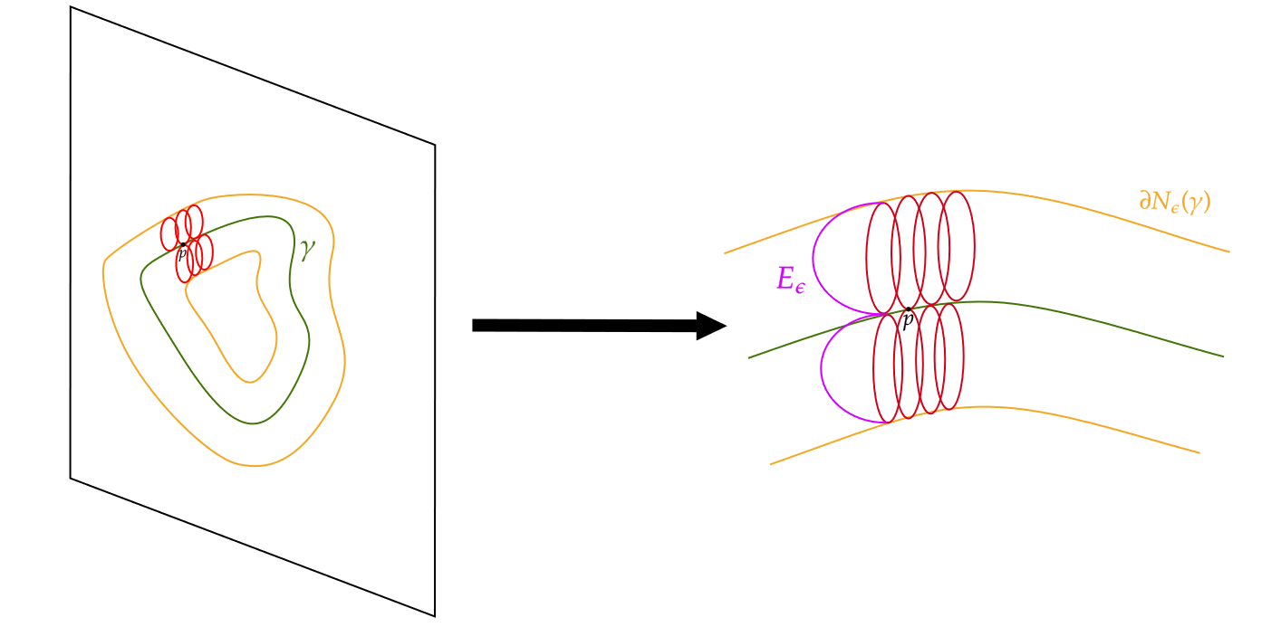
Figure 6: Envelope Construction

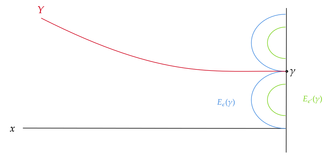
Figure 7: $\epsilon^{\prime}<\epsilon$ argument

Keeping the centers of each hemisphere fixed, shrink the radius of each to form $E_{\epsilon^{\prime}}$ for $\epsilon^{\prime}<\epsilon$ (cf. figure 7). This is still a mean-convex smooth hypersurface. Now if

$$\exists\epsilon^{\prime}<\epsilon\;\text{ s.t. }\;E_{\epsilon^{\prime}}\cap Y\neq\emptyset$$

then using $\epsilon^{\prime}<\epsilon$, we see that they intersect at $p$ with $x(p)>0$. By the maximum principle for mean-convex surfaces (see [20], [29]), for some open neighborhood $V\subseteq Y$, we have that $V\subseteq E_{\epsilon^{\prime}}$. Because this is an open condition and $E_{\epsilon^{\prime}}$ is connected, we see that $Y\cap\{x<\epsilon^{\prime}\}\subseteq E_{\epsilon^{\prime}}$ so that in particular $\gamma\subseteq E_{\epsilon^{\prime}}$ by continuity (recall that $Y$ is embedded in $M$ in a neighborhood of $\gamma$). But this is a contradiction to $\epsilon^{\prime}<\epsilon$, so the smaller envelopes $\{E_{\epsilon^{\prime}}\}$ do not intersect $Y$ near the boundary. Now for each

$$p\in E_{\epsilon}$$

we can express them locally as

$$p\leftrightarrow(s,x,z^{i}=v^{i}(s,x))$$

By construction of the envelope, we know that

$$|v^{i}(s,x)|\leq\frac{x^{2}}{\epsilon}$$

Moreover, $Y$ is surrounded by the envelope as we approach the boundary, i.e. if we represent

$$\begin{gathered}q\in Y,\qquad q=\gamma(s)+u^{i}(s,x)\overline{N}_{i}(s)\\ \implies|u^{i}(s,x)|\leq|v^{i}(s,x)|\qquad\forall x<\epsilon\end{gathered}$$

which implies

$$\boxed{||u(s,x)||\leq\frac{m}{\epsilon}x^{2}}$$

for some $\epsilon>0$ and for all $x<\epsilon$. This shows that $Y$ approaches the boundary quadratically (see figure 8).

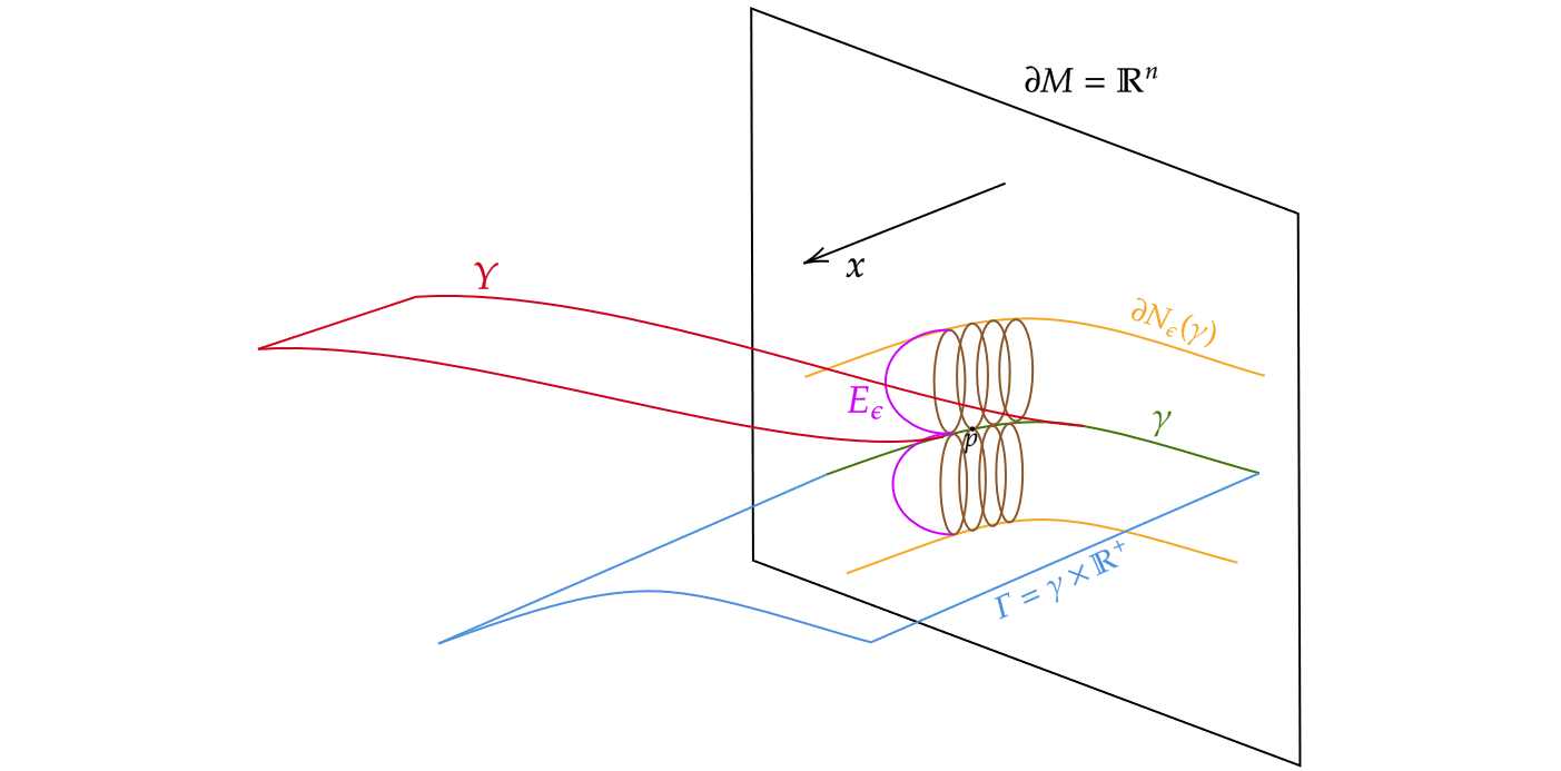
Figure 8:

13.8 Degeneracy of Minimal Hypersurfaces in $M^{n+1}$

In this section, we summarize the relevant results from section $4$ of [2] on the degeneracy of a minimal submanifold $Y^{m}\subseteq M$. For $X\in N(Y)$, recall the Jacobi operator:

$$J_{Y}(X)=\Delta^{\perp}_{Y}(X)+\tilde{A}(X)-\text{Tr}_{TY}[R(\cdot,X)\cdot]$$

We can view $J_{Y}$ as a map between weighted Hölder spaces

$$J_{Y}:x^{\mu}\Lambda^{2,\alpha}_{0}(N(Y))\to x^{\mu}\Lambda^{0,\alpha}_{0}(N(Y))$$

Moreover, the indicial roots of this operator are $\mu_{1}=-1$ and $\mu_{2}=m$. When $-1<\mu<m$, we know from [26] that $J_{Y}$ is Fredholm and index $0$ in the codimension $1$ case. A minimal submanifold $Y^{m}\subseteq M$ is said to be nondegenerate if the kernel of this map is just $\{0\}$. Again in the codimension $1$ case, one can show that any boundary variation of a nondegenerate submanifold, i.e.

$$\gamma_{\psi}=\{\overline{\exp}_{p}(\psi(p)N(p))\},\qquad\psi\in C^{\infty}(\gamma)$$

can be extended to a Jacobi field on $Y$, $X=\dot{\phi}(p,x)\nu(p,x)$, so that $\dot{\phi}(p,0)=\psi(p)$. This follows by an inverse function theorem argument which is a direct adaption of the $n=2$ case described in [26].

When $Y$ is degenerate, $L_{Y}$ is still index $0$ but the kernel is a non-trivial finite dimensional space. We consider the kernel of $L_{Y}$ acting on functions $\psi\in L^{2}$, i.e. such that $\psi_{0}=0$,

$$K=\{\psi\;|\;J_{Y}(\psi)=0,\;\psi_{0}=0\}$$

Elements of $K$ have the following asymptotic expansion:

$$\psi\sim\begin{cases}\psi_{m+1}(s)x^{m+1}+\dots&m\text{ even}\\ \psi_{m+1}(s)x^{m+1}+\Psi(s)x^{m+1}\log(x)+\dots&m\text{ odd}\end{cases}$$

i.e. they vanish to order $m+1$. Consider

$$V=\{f\;|\;\exists\psi\in K\;\text{ s.t. }\;f=\psi_{n+1}\}$$

which is also finite dimensional. Recall equation (28), i.e. for $Y^{n}$ a critical point of renormalized volume and $n$ even, we have

$$\int_{\gamma}u_{n+1}(s)\dot{\phi}_{0}(s)dA_{\gamma}=0$$

From the above, if $\dot{\phi}_{0}(s)\leftrightarrow\phi(s,x)$ a Jacobi field, and $\psi_{n+1}(s)\leftrightarrow\psi(s,x)$ an $L^{2}$ Jacobi field, then

$$0 =\int_{Y}J_{Y}(\phi(s,x))\psi(s,x)dA_{Y}$$

$$=\int_{Y}[(\Delta_{Y}\phi)\psi+|A_{Y}|^{2}\phi\psi-\text{Ric}_{TY}(\nu,\nu)\phi\psi]dA_{Y}$$

$$=\int_{Y}[(\Delta_{Y}\psi)\phi+|A_{Y}|^{2}\psi\phi-\text{Ric}_{TY}(\nu,\nu)\psi\phi]dA_{Y}-\int_{\gamma}(n+1)(\psi_{n+1})\dot{\phi}_{0}dA_{\gamma}$$

$$=\int_{Y}J_{Y}(\psi)\phi-(n+1)\int_{\gamma}\psi_{n+1}\dot{\phi}_{0}dA_{\gamma}$$

$$=-(n+1)\int\psi_{n+1}\dot{\phi}_{0}dA_{\gamma}$$

The equality in line three is most easily seen by switching to the compactified metric, keeping track of powers of $x$, and integrating by parts twice. This tells us that $\dot{\phi}_{0}(s)$ must be orthogonal to all elements of $V$, i.e. $\langle\dot{\phi}_{0}(s),f\rangle_{L^{2}(\gamma)}=0$. This then tells us that any $u_{n+1}\in V$ lies in a finite dimensional space.

13.9 Computing $\overline{h}_{n+1}^{xx}$ and $\overline{q}_{n+1}$

In this section, we consider $Y^{n}\subseteq M^{n+1}$ and compute the $(n+1)$st coefficient for the metric coefficient $\overline{h}^{xx}(s,x)$ and the volume form prefactor $\overline{q}(s,x)$. We aim to show

Proposition.

For $Y^{n}\subseteq M^{n+1}$ minimal, we have

$$\overline{h}^{xx}_{n+1}+\overline{q}_{n+1}=\begin{cases}(n-1)(n-2)-4(3n-1)u_{2}u_{n+1}+\text{Tr}_{T\gamma}(k_{n+1,0})&n\text{ even}\\ (n-1)(n-2)-4(3n-1)u_{2}u_{n+1}+\text{Tr}_{T\gamma}(k_{n+1,0})+R(u_{2})&n\text{ odd}\end{cases}$$

where

$$k_{n+1,0}:=\frac{1}{(n+1)!}\left(\frac{d}{dx}\right)^{n+1}k(s,x,0)\Big{|}_{x=0}$$

Remark  When $M=\mathbb{H}^{n+1}/\Gamma$ for $\Gamma$ a coconvex subgroup, $k_{n+1}=0$.

13.9.1 $\overline{h}_{n+1}^{xx}$, even

Expansion by minors of the inverse yields

$$\overline{h}^{xx}=\frac{1}{\det\overline{h}}\det(\{\overline{h}_{ab}\})$$

where $a,b=1,\dots,n-1$ are the coordinates corresponding to coordinates for $s$. Note that $\mathcal{F}(\overline{h}_{ab})=1$ via

$$v_{a} =\partial_{s_{a}}+\overline{\Gamma}_{az}^{\alpha}u\partial_{y_{\alpha}}+u_{a}\partial_{z}$$

$$=\partial_{s_{a}}+\overline{\Gamma}_{az}^{b}u\partial_{s_{b}}+\overline{\Gamma}_{az}^{x}u\partial_{x}+u_{a}\partial_{z}$$

$$\overline{h}_{ab} =\overline{g}_{ab}+u_{b}\overline{g}_{az}+u\overline{\Gamma}_{bz}^{\beta}\overline{g}_{a\beta}$$

$$+u_{a}\overline{g}_{bz}+u_{a}u_{b}\overline{g}_{zz}+u_{a}u\overline{\Gamma}_{bz}^{\beta}\overline{g}_{z\beta}$$

$$+u\overline{\Gamma}_{az}^{\alpha}\overline{g}_{b\alpha}+u_{b}u\overline{\Gamma}_{az}^{\alpha}\overline{g}_{z\alpha}+u^{2}\overline{\Gamma}_{az}^{\alpha}\overline{\Gamma}_{bz}^{\beta}\overline{g}_{\alpha\beta}$$

where $\overline{\Gamma}_{\sigma\mu}^{\tau}$ is the Christoffel symbol as in lemma 25. Similarly, we have that

$$\det\overline{h} =1+x^{2}\overline{q}_{2}+\dots+x^{n}\overline{q}_{n}+x^{n}\log(x)\overline{Q}+x^{n+1}\overline{q}_{n+1}+O(x^{n+2}\log(x))$$

$$\implies\frac{1}{\det\overline{h}} =1+(\text{even terms up to order $n$})-\overline{Q}x^{n}\log(x)-\overline{q}_{n+1}x^{n+1}+O(x^{n+2})$$

Because $\mathcal{F}(\det(\{\overline{h}_{ab}\}))=1$, we can compute

$$\overline{h}^{xx}_{n+1} =\left([\det\overline{h}]^{-1}\right)_{n+1}\cdot\left(\det(\{\overline{h}_{ab}\})\right)_{0}+\left([\det\overline{h}]^{-1}\right)_{0}\cdot\left(\det(\{\overline{h}_{ab}\})\right)_{n+1}$$

$$=-\overline{q}_{n+1}+(\det\{\overline{h}_{ab}\})_{n+1}$$

Now note that we can write

$$\overline{h}_{ab}=(\overline{h}_{ab})_{0}+(\overline{h}_{ab})_{2}x^{2}+(\text{even terms})+(\overline{h}_{ab})_{n}x^{n}+(\overline{h}^{*}_{ab})x^{n}\log(x)+(\overline{h}_{ab})_{n+1}x^{n+1}+\dots$$

Because $\mathcal{F}(\overline{h}_{ab})=1$, we use linearity of the determinant to get

$$\left(\det(\{\overline{h}_{ab}\})\right)_{n+1}=\sum_{a,b=1}^{n-1}\begin{vmatrix}(\overline{h}_{11})_{0}&\cdots&(\overline{h}_{1\;(n-1)})_{0}\\ \cdots&(\overline{h}_{ab})_{(n+1)}&\cdots\\ (\overline{h}_{(n-1)\;1})_{0}&\cdots&(\overline{h}_{(n-1)\;(n-1)})_{0}\end{vmatrix}$$

i.e. all of the matrix terms take $0$th order coefficients except for $\overline{g}_{ij}$, which takes the $n+1$st coefficient. Fortunately, we know that

$$(\overline{h}_{ab})_{0}=\delta_{ab}$$

so the above can be thought of as the identity matrix with the $(i,j)$th entry substituted with $\overline{h}_{ij}$. Note that the determinant of such a matrix is

$$\begin{vmatrix}1&\cdots&0\\ \cdots&(\overline{h}_{ab})_{(n+1)}&\cdots\\ 0&\cdots&1\end{vmatrix}=\begin{cases}1&i\neq j\\ (\overline{h}_{aa})_{n+1}&a=b\end{cases}$$

but note that in our expansion of

$$\overline{h}_{aa} =\overline{g}_{aa}+2u_{a}\overline{g}_{az}+2u\overline{\Gamma}_{az}^{d}\overline{g}_{ad}+u_{a}^{2}\overline{g}_{zz}$$

$$+2u_{a}u\overline{\Gamma}_{az}^{d}\overline{g}_{zd}+u^{2}\overline{\Gamma}_{az}^{c}\overline{\Gamma}_{az}^{d}\overline{g}_{cd}$$

We see that all of the christoffel symbols and metric terms satisfy $\mathcal{F}(\cdot)=1$. Moreover $u$, $u_{a}$ are both $O(x^{2})$ and $\overline{g}_{az}\Big{|}_{Y}=O(x^{4})$, so we can compute

$$[\overline{h}_{aa}]^{n+1} =[\overline{g}_{aa}]^{n+1}+2[u\overline{\Gamma}_{az}^{a}\overline{g}_{aa}]^{n+1}$$

$$=[\overline{g}_{aa}]^{n+1}+2[u]^{n+1}\cdot[\overline{\Gamma}_{az}^{a}\overline{g}_{aa}]^{0}$$

To compute $\overline{g}_{aa}$ we first recall the expansion of $k_{0}(s,z)$ in

$$\overline{g} =dx^{2}+k_{0}(s,z)+x^{2}k_{2}(s,z)+\dots+k_{n}(s,z)x^{n}+K(s,z)x^{n}\log(x)+k_{n+1}(s,z)x^{n+1}$$

$$k_{i}(s,z) =k_{i,0}(s)+k_{i,1}(s)z+\dots+k_{i,n/2}(s)z^{n/2}+O(z^{n/2+1})$$

$$K(s,z) =K_{0}(s)+k_{1}(s)z+\dots+k_{n/2}(s)z^{n/2}+O(z^{n/2+1})$$

when we evaluate at $z=u=O(x^{2})$, we see that

$$[\overline{g}_{aa}]^{n+1} =[k_{0}(s,z=u)(\partial_{s_{a}},\partial_{s_{a}})]^{n+1}+[k_{n+1}(s,z=u)(\partial_{s_{a}},\partial_{s_{a}})]^{0}$$

$$=[k_{0}(s,z=u)(\partial_{s_{a}},\partial_{s_{a}})]^{n+1}+k_{n+1,0}(\partial_{s_{a}},\partial_{s_{a}})$$

because $\mathcal{F}(u)=1$. Of course, from (31) or [22]

$$k_{0}(s,z)(\partial_{s_{a}},\partial_{s_{b}})=\delta_{ab}+[\overline{\overline{\Gamma}}_{ab}^{z}+\overline{\overline{\Gamma}}_{ba}^{z}]z+O(z^{2},sz,s^{2})$$

where $\overline{\overline{\Gamma}}_{\cdot\cdot}^{\cdot}$ are the Christoffels as in equation (31). When evaluated at $z=u$ and $s=0$, the $O(z^{2},sz,s^{2})$ terms will not contribute a $n+1$st term. Thus

$$[k_{0}(s,z=u)]^{n+1}=-2\overline{\Gamma}_{\gamma,aaz}u_{n+1}$$

where $\overline{\Gamma}_{\gamma,\cdot}$ denotes the restriction of the christoffels in lemma 4.2 restricted to $T\gamma$. We leave the other term as is and get

$$[\overline{g}_{aa}]^{n+1} =-2\overline{\Gamma}_{\gamma,aaz}u_{n+1}+k_{n+1,0}$$

Similarly

$$2(u\overline{\Gamma}_{az}^{a}|_{Y})_{n+1}=2u_{n+1}\overline{\Gamma}_{\gamma,aza}=-2u_{n+1}\overline{\Gamma}_{\gamma,aaz}$$

so that

$$[\overline{h}_{aa}]^{n+1}=-4u_{n+1}\overline{\Gamma}_{\gamma,aaz}+k_{n+1,0}(\partial_{s_{a}},\partial_{s_{a}})$$

With this, we get

$$\left(\det(\{\overline{h}_{ab}\})\right)_{n+1} =\sum_{a,b=1}^{n-1}\begin{vmatrix}(\overline{h}_{11})_{0}&\cdots&(\overline{h}_{1\;(n-1)})_{0}\\ \cdots&(\overline{h}_{ab})_{(n+1)}&\cdots\\ (\overline{h}_{(n-1)\;1})_{0}&\cdots&(\overline{h}_{(n-1)\;(n-1)})_{0}\end{vmatrix}$$

$$=(n-1)^{2}-(n-1)+\sum_{a=1}^{n-1}[-4u_{n+1}\overline{\Gamma}_{\gamma,aaz}+k_{n+1,0}(\partial_{s_{a}},\partial_{s_{a}})]$$

$$=(n-1)(n-2)-4u_{n+1}H_{\gamma,k_{0}}+\text{Tr}_{T\gamma}(k_{n+1,0})$$

to get this expression we reason as follows: when $a\neq b$, we have the identity matrix and one off diagonal term which is $(\overline{h}_{ab})_{n+1})$. The determinant of this matrix is still $1$, and this occurs $(n-1)^{2}-(n-1)$ times. When $a=b$, we get the identity with one diagonal entry replaced by $(\overline{h}_{aa})_{n+1}$ giving us the result. Now using the fact that $H_{\gamma,k_{0}}=2(n-1)u_{2}$, we get

$$\boxed{\overline{h}^{xx}_{n+1}=-\overline{q}_{n+1}+(n-1)(n-2)-8(n-1)u_{2}u_{n+1}+\text{Tr}_{T\gamma}(k_{n+1,0})}$$

13.9.2 $\overline{h}_{n+1}^{xx}+\overline{q}_{n+1}$, odd

Via the same reasoning as in the even case, we have that

$$\overline{h}_{n+1}^{xx}+\overline{q}_{n+1}=(\det\{\overline{h}_{ab}\})_{n+1}+R(u_{2})$$

where $R$ is some function of $u_{2}$ and its derivatives. Expanding this determinant and using multilinearity, we have

$$(\det\{\overline{h}_{ab}\})_{n+1}=\sum_{a,b=1}^{n-1}\begin{vmatrix}(\overline{h}_{11})_{0}&\cdots&(\overline{h}_{1\;(n-1)})_{0}\\ \cdots&(\overline{h}_{ab})_{(n+1)}&\cdots\\ (\overline{h}_{(n-1)\;1})_{0}&\cdots&(\overline{h}_{(n-1)\;(n-1)})_{0}\end{vmatrix}+R(u_{2})$$

so that

$$\left(\det(\{\overline{h}_{ab}\})\right)_{n+1} =(n-1)(n-2)-8(n-1)u_{2}u_{n+1}+\text{Tr}_{T\gamma}(k_{n+1,0})+R(u_{2})$$

$$\implies\overline{h}_{n+1}^{xx}+\overline{q}_{n+1} =(n-1)(n-2)-8(n-1)u_{2}u_{n+1}+\text{Tr}_{T\gamma}(k_{n+1,0})+R(u_{2})$$

13.10 Second variation of Mean Curvature - Parity for $\ddot{S}$

In this section, we compute the second variation of mean curvature for a family of minimal surfaces $\{Y_{t}\}$ and prove theorem 5.2 and proposition 2

Theorem.

Let $\{Y_{t}\}\subseteq M^{n+1}$ be a family of minimal of $m$-dimensional minimal submanifolds. Let $Y=Y_{0}$ and $\overline{h}$ denote a compactified metric on $Y$. Then for

$$Y_{t}=\{\exp_{\overline{h},p}(S_{t}(p)\overline{\nu}(p))\;|\;p\in Y\}$$

and $\{w_{i}\}$ the normal basis described in section §13.3, we have

$$\ddot{S}=\frac{d^{2}}{dt^{2}}\Big{|}_{t=0}S_{t}=\ddot{S}^{i}w_{i}$$

and $\mathcal{F}(\ddot{S}^{i})=1$.

Proposition.

Let $\{Y_{t}^{m}\}\subseteq M^{n+1}$ be a family of minimal of $m$-dimensional minimal submanifolds. Let $Y=Y_{0}$ and $\overline{h}$ denote a compactified metric on $Y$. Then for

$$Y_{t}=\{\exp_{\overline{h},p}(S_{t}(p))\;|\;p\in Y\}$$

The second variation of mean curvature is given by

$$\frac{d^{2}}{dt^{2}}H_{t}=J_{Y}^{\perp}(\ddot{S})+Q^{\perp}(\dot{S})$$

where $Q^{\perp}$ is a quadratic differential functional in $\dot{S}$ and

$$Q^{\perp}(\dot{S}) =Q^{i}(s,x)w_{i}$$

$$\mathcal{F}(Q^{i}) =1$$

13.10.1 Normality of $\ddot{S}$

We first show that $\ddot{S}=\nabla_{F_{t}}F_{t}\Big{|}_{t=0}\in NY$ since $F_{t}$ is a normal variation. Recall that the image of $\sigma_{p}(t)=F(p,t)$ is a geodesic curve starting at $p$. We write

$$F_{*}(\partial_{t})\Big{|}_{q=\sigma_{p}(t)}=F_{t}\Big{|}_{q=\sigma_{p}(t)}=A(t)\tau(t)\Big{|}_{q=\sigma_{p}(t)}$$

for $\tau(t)$ a unit normal tangent vector evaluated at $q=F_{t}(p)$ on the path produced by $F_{t}(p)$. We compute

$$\ddot{S}(p) =\nabla_{F_{t}}F_{t}\Big{|}_{t=0}$$

$$=(A(t)\tau(t))(A(t))\Big{|}_{t=0}\;\tau(0)+A^{2}(0)\nabla_{\tau(t)}\tau(t)\Big{|}_{t=0}$$

$$=\dot{A}\tau$$

where the second term vanishes since $\nabla_{\tau}\tau=0$ since $\tau$ is the tangent vector to a geodesic curve. But $\tau(0)\in NY$, so $\ddot{S}\in NY$.

13.10.2 Proof of theorems 5.2 and 2

We have for some $t_{0}>0$:

$$\forall t\in[0,t_{0}),\qquad H(t)=0=h^{\alpha\beta}(t)A_{\alpha\beta}(t)=0$$

here, $h_{\alpha\beta}(t)$ is the induced metric on $Y_{t}$ from the ambient $(M,g)$ and $A_{\alpha\beta}(t)$ the induced second fundamental form, taking values in $NY_{t}$. We can differentiate the above twice and get

$$\ddot{h}^{\alpha\beta}A_{\alpha\beta}+\dot{h}^{\alpha\beta}\dot{A}_{\alpha\beta}^{i}+h^{\alpha\beta}\ddot{A}_{\alpha\beta}^{i}=0$$

We recall

$$\dot{h}^{\alpha\beta} =-h^{\alpha\gamma}\dot{h}_{\gamma\delta}h^{\delta\beta}$$

$$\ddot{h}^{\alpha\beta} =2h^{\alpha\gamma}\dot{h}_{\gamma\delta}h^{\delta\kappa}\dot{h}_{\kappa\ell}h^{\ell\beta}-h^{\alpha\gamma}\ddot{h}_{\gamma\delta}h^{\delta\beta}$$

so we compute the derivatives of $h$ and $A$.

13.10.2.1 $\ddot{h}$

Similarly, we have that

$$\ddot{h} =F_{t}F_{t}g(F_{\alpha},F_{\beta})$$

$$=g(\nabla_{F_{t}}\nabla_{F_{t}}F_{\alpha},F_{\beta})+2g(\nabla_{F_{t}}F_{\alpha},\nabla_{F_{t}}F_{\beta})+g(F_{\alpha},\nabla_{F_{t}}\nabla_{F_{t}}F_{\beta})$$

$$=I_{1}+I_{2}+I_{3}$$

And so we handle these terms separately to show

$$\ddot{h}_{\alpha\beta} =2\left[-\ddot{S}^{i}A_{\alpha\beta i}+\dot{S}^{i}\dot{S}^{j}R_{i\alpha j\beta}\right]$$

$$+2\left[\dot{S}^{i}_{\alpha}\dot{S}^{j}_{\beta}g_{ij}+\dot{S}^{i}\dot{S}^{j}_{\beta}A_{\alpha ij}+\dot{S}^{j}\dot{S}^{i}_{\alpha}A_{\beta ji}+\dot{S}^{i}\dot{S}^{j}(\Gamma\circ\Gamma)_{\alpha i\beta j}\right]$$

For the raised version, we have

$$\ddot{h}^{\alpha\beta} =2h^{\alpha\gamma}\dot{h}_{\gamma\delta}h^{\delta\kappa}\dot{h}_{\kappa\ell}h^{\ell\beta}-h^{\alpha\gamma}\ddot{h}_{\gamma\delta}h^{\delta\beta}$$

$$=4\dot{S}^{i}\dot{S}^{j}(A\circ A)^{\alpha\beta}_{ij}$$

$$+2\left[-\ddot{S}^{i}A^{\alpha\beta}_{i}+\dot{S}^{i}\dot{S}^{j}R_{ij}^{\alpha\beta}\right]$$

$$+2\left[\dot{S}^{i,\alpha}\dot{S}^{j,\beta}g_{ij}+\dot{S}^{i}\dot{S}^{j,\beta}\Gamma_{ij}^{\alpha}+\dot{S}^{j}\dot{S}^{i,\alpha}\Gamma^{\beta}_{ji}+\dot{S}^{i}\dot{S}^{j}(\Gamma\circ\Gamma)^{\alpha\beta}_{ij}\right]$$

13.10.2.1.1 $I_{1}$

We compute

$$I_{1} =g(\nabla_{F_{t}}\nabla_{F_{t}}F_{\alpha},F_{\beta})$$

$$=g(\nabla_{F_{t}}\nabla_{F_{\alpha}}F_{t},F_{\beta})$$

$$=R(F_{t},F_{\alpha},F_{t},F_{\beta})+g(\nabla_{F_{\alpha}}\nabla_{F_{t}}F_{t},F_{\beta})$$

$$=R(\dot{S}^{i}\nu_{i},v_{\alpha},\dot{S}^{j}\nu_{j},v_{\beta})+g(\nabla_{v_{\alpha}}\ddot{S}^{i}\nu_{i},v_{\beta})$$

$$=\dot{S}^{i}\dot{S}^{j}R_{\nu_{i}\alpha\nu_{j}\beta}+\ddot{S}^{i}g(\nabla_{v_{\alpha}}\nu_{i},v_{\beta})$$

$$=\dot{S}^{i}\dot{S}^{j}R_{\nu_{i}\alpha\nu_{j}\beta}-\ddot{S}^{i}A_{\alpha\beta i}$$

13.10.2.1.2 $I_{2}$

We have

$$I_{2} =2g(\nabla_{F_{t}}F_{\alpha},\nabla_{F_{t}}F_{\beta})$$

$$=2g(\nabla_{F_{\alpha}}F_{t},\nabla_{F_{\beta}}F_{t})$$

$$=2g(\nabla_{v_{\alpha}}\dot{S}^{i}\nu_{i},\nabla_{v_{\beta}}\dot{S}^{j}\nu_{j})$$

$$=2g(\dot{S}^{i}_{\alpha}\nu_{i}+\dot{S}^{i}\nabla_{v_{\alpha}}\nu_{i},\dot{S}^{j}_{\beta}\nu_{j}+\dot{S}^{j}\nabla_{v_{\beta}}\nu_{j})$$

$$=2\left[\dot{S}^{i}_{\alpha}\dot{S}^{j}_{\beta}g_{ij}+\dot{S}^{i}\dot{S}^{j}_{\beta}\Gamma_{\alpha ij}+\dot{S}^{j}\dot{S}^{i}_{\alpha}\Gamma_{\beta ji}+\dot{S}^{i}\dot{S}^{j}\Gamma_{\alpha i}^{\sigma}\Gamma_{\beta j}^{\tau}g_{\sigma\tau}\right]$$

$$=2\left[\dot{S}^{i}_{\alpha}\dot{S}^{j}_{\beta}g_{ij}+\dot{S}^{i}\dot{S}^{j}_{\beta}\Gamma_{\alpha ij}+\dot{S}^{j}\dot{S}^{i}_{\alpha}\Gamma_{\beta ji}+\dot{S}^{i}\dot{S}^{j}(\Gamma\circ\Gamma)_{\alpha i\beta j}\right]$$

13.10.2.1.3 $I_{3}$

This is the same as $I_{1}$ and will give

$$I_{3}=\dot{S}^{i}\dot{S}^{j}R_{\nu\beta\nu\alpha}-\ddot{S}^{i}A_{\beta\alpha i}=I_{1}$$

by symmetry.

13.10.2.2 $\ddot{A}_{\alpha\beta}$

Again, we compute using the definition

$$A_{\alpha\beta}(t) =\nabla_{F_{\alpha}}F_{\beta}-h^{\gamma\delta}g(\nabla_{F_{\alpha}}F_{\beta},F_{\gamma})F_{\delta}$$

$$\ddot{A}_{\alpha\beta} =\nabla_{F_{t}}\nabla_{F_{t}}[\nabla_{F_{\alpha}}F_{\beta}-h^{\gamma\delta}g(\nabla_{F_{\alpha}}F_{\beta},F_{\gamma})F_{\delta}]$$

$$=\nabla_{F_{t}}\left(R(F_{t},F_{\alpha},F_{\beta})+\nabla_{F_{\alpha}}\nabla_{F_{t}}F_{\beta}\right)-\nabla_{F_{t}}\nabla_{F_{t}}[h^{\gamma\delta}g(\nabla_{F_{\alpha}}F_{\beta},F_{\gamma})F_{\delta}]$$

$$=I_{1,\alpha\beta}+I_{2,\alpha\beta}$$

we break these down as follows

13.10.2.2.1 $I_{1,\alpha\beta}$

We have

$$\nabla_{F_{t}}R(F_{t},F_{\alpha},F_{\beta}) =(\nabla_{F_{t}}R)(F_{t},F_{\alpha},F_{\beta})+R(\nabla_{F_{t}}F_{t},F_{\alpha},F_{\beta})+R(F_{t},\nabla_{F_{t}}F_{\alpha},F_{\beta})+R(F_{t},F_{\alpha},\nabla_{F_{t}}F_{\beta})$$

$$=(\nabla_{\dot{S}}R)(\dot{S},v_{\alpha},v_{\beta})+R(\ddot{S},v_{\alpha},v_{\beta})+R(\dot{S},\nabla_{v_{\alpha}}\dot{S},v_{\beta})+R(\dot{S},v_{\alpha},\nabla_{v_{\beta}}\dot{S})$$

Similarly

$$\nabla_{F_{t}}\nabla_{F_{\alpha}}\nabla_{F_{t}}F_{\beta} =\nabla_{F_{t}}\nabla_{F_{\alpha}}\nabla_{F_{\beta}}F_{t}$$

$$=R(F_{t},F_{\alpha},\nabla_{F_{\beta}}F_{t})+\nabla_{F_{\alpha}}\nabla_{F_{t}}\nabla_{F_{\beta}}F_{t}$$

$$=R(\dot{S},v_{\alpha},\nabla_{v_{\beta}}\dot{S})+\nabla_{F_{\alpha}}[R(\dot{S},v_{\beta},\dot{S})+\nabla_{F_{\beta}}\ddot{S}]$$

$$=R(\dot{S},v_{\alpha},\nabla_{v_{\beta}}\dot{S})$$

$$+(\nabla_{v_{\alpha}}R)(\dot{S},v_{\beta},\dot{S})+R(\nabla_{v_{\alpha}}\dot{S},v_{\beta},\dot{S})+A_{\alpha\beta}^{i}R(\dot{S},\nu_{i},\dot{S})+R(\dot{S},v_{\beta},\nabla_{v_{\alpha}}\dot{S})$$

$$+\nabla_{F_{\alpha}}\nabla_{F_{\beta}}\ddot{S}$$

After using the first bianchi identity, we write this as

$$I_{1} =\nabla_{v_{\alpha}}\nabla_{v_{\beta}}\ddot{S}+R(\ddot{S},v_{\alpha},v_{\beta})+(\nabla_{\dot{S}}R)(\dot{S},v_{\alpha},v_{\beta})+(\nabla_{v_{\alpha}}R)(\dot{S},v_{\beta},\dot{S})$$

$$+2R(\dot{S},v_{\alpha},\nabla_{v_{\beta}}\dot{S})+2R(\dot{S},v_{\beta},\nabla_{v_{\alpha}}\dot{S})+A_{\alpha\beta}^{i}R(\dot{S},\nu_{i},\dot{S})$$

13.10.2.3 $I_{2,\alpha\beta}$

We have

$$\nabla_{F_{t}}\nabla_{F_{t}}[h^{\gamma\delta}g(\nabla_{F_{\alpha}}F_{\beta},F_{\gamma})F_{\delta}] =\nabla_{F_{t}}[\dot{h}^{\gamma\delta}g(\nabla_{F_{\alpha}}F_{\beta},F_{\gamma})F_{\delta}+h^{\gamma\delta}g(\nabla_{F_{t}}\nabla_{F_{\alpha}}F_{\beta},F_{\gamma})F_{\delta}$$

$$+h^{\gamma\delta}g(\nabla_{F_{\alpha}}F_{\beta},\nabla_{F_{t}}F_{\gamma})F_{\delta}+h^{\gamma\delta}g(\nabla_{F_{\alpha}}F_{\beta},F_{\gamma})\nabla_{F_{t}}F_{\delta}]$$

$$=I_{21,\alpha\beta}+I_{22,\alpha\beta}+I_{23,\alpha\beta}+I_{24,\alpha\beta}$$

13.10.2.3.1 $I_{21,\alpha\beta}$

We compute

$$I_{21,\alpha\beta} =\ddot{h}^{\gamma\delta}g(\nabla_{F_{\alpha}}F_{\beta},F_{\gamma})F_{\delta}+\dot{h}^{\gamma\delta}g(\nabla_{F_{t}}\nabla_{F_{\alpha}}F_{\beta},F_{\gamma})F_{\delta}$$

$$+\dot{h}^{\gamma\delta}g(\nabla_{F_{\alpha}}F_{\beta},\nabla_{F_{t}}F_{\gamma})F_{\delta}+\dot{h}^{\gamma\delta}g(\nabla_{F_{\alpha}}F_{\beta},F_{\gamma})\nabla_{F_{t}}F_{\delta}$$

$$=\ddot{h}^{\gamma\delta}\Gamma_{\alpha\beta\gamma}v_{\delta}$$

$$+\dot{h}^{\gamma\delta}[R(\dot{S},v_{\alpha},v_{\beta},v_{\gamma})+g(\nabla_{v_{\alpha}}\nabla_{v_{\beta}}\dot{S},v_{\gamma})+A_{\alpha\beta j}\dot{S}^{j}_{\gamma}]v_{\delta}$$

$$+\dot{h}^{\gamma\delta}\Gamma_{\alpha\beta\gamma}\nabla_{v_{\gamma}}\dot{S}$$

noting that $\Gamma_{\alpha\beta\gamma}=0$ by choice of fermi coordinates and using $\dot{h}^{\gamma\delta}=-2\dot{S}^{i}A_{i}^{\gamma\delta}$, we have

$$I_{21,\alpha\beta} =-2\dot{S}^{i}A^{\gamma\delta}_{i}[R(\dot{S},v_{\alpha},v_{\beta},v_{\gamma})+g(\nabla_{v_{\alpha}}\nabla_{v_{\beta}}\dot{S},v_{\gamma})+A_{\alpha\beta j}\dot{S}^{j}_{\gamma}]v_{\delta}$$

13.10.2.3.2 $I_{22,\alpha\beta}$

Similarly, we have

$$I_{22,\alpha\beta} =\dot{h}^{\gamma\delta}g(\nabla_{F_{t}}\nabla_{F_{\alpha}}F_{\beta},F_{\gamma})F_{\delta}+h^{\gamma\delta}g(\nabla_{F_{t}}\nabla_{F_{t}}\nabla_{F_{\alpha}}F_{\beta},F_{\gamma})F_{\delta}$$

$$+h^{\gamma\delta}g(\nabla_{F_{t}}\nabla_{F_{\alpha}}F_{\beta},\nabla_{F_{t}}F_{\gamma})F_{\delta}+h^{\gamma\delta}g(\nabla_{F_{t}}\nabla_{F_{\alpha}}F_{\beta},F_{\gamma})\nabla_{F_{t}}F_{\delta}$$

As before, we know that

$$\dot{h}^{\gamma\delta}g(\nabla_{F_{t}}\nabla_{F_{\alpha}}F_{\beta},F_{\gamma})F_{\delta}=-2\dot{S}^{i}A^{\gamma\delta}_{i}[R(\dot{S},v_{\alpha},v_{\beta},v_{\gamma})+g(\nabla_{v_{\alpha}}\nabla_{v_{\beta}}\dot{S},v_{\gamma})]v_{\delta}$$

We can compute

$$\nabla_{F_{t}}\nabla_{F_{t}}\nabla_{F_{\alpha}}F_{\beta} =(\nabla_{\dot{S}}R)(\dot{S},v_{\alpha},v_{\beta})+R(\ddot{S},v_{\alpha},v_{\beta})+R(\dot{S},\nabla_{v_{\alpha}}\dot{S},v_{\beta})+2R(\dot{S},v_{\alpha},\nabla_{v_{\beta}}\dot{S})$$

$$+(\nabla_{v_{\alpha}}R)(\dot{S},v_{\beta},\dot{S})+R(\nabla_{v_{\alpha}}\dot{S},v_{\beta},\dot{S})+A_{\alpha\beta}^{i}R(\dot{S},\nu_{i},\dot{S})+R(\dot{S},v_{\beta},\nabla_{v_{\alpha}}\dot{S})+\nabla_{v_{\alpha}}\nabla_{v_{\beta}}\ddot{S}$$

Moreover

$$g(\nabla_{F_{t}}\nabla_{F_{\alpha}}F_{\beta},\nabla_{F_{t}}F_{\gamma}) =R(\dot{S},v_{\alpha},v_{\beta},\nabla_{v_{\gamma}}\dot{S})+g(\nabla_{v_{\alpha}}\nabla_{v_{\beta}}\dot{S},\nabla_{v_{\gamma}}\dot{S})$$

And finally

$$g(\nabla_{F_{t}}\nabla_{F_{\alpha}}F_{\beta},F_{\gamma})\nabla_{F_{t}}F_{\delta} =[R(\dot{S},v_{\alpha},v_{\beta},v_{\gamma})+g(\nabla_{v_{\alpha}}\nabla_{v_{\beta}}\dot{S},v_{\gamma})]\nabla_{v_{\delta}}\dot{S}$$

So that

$$I_{22,\alpha\beta} =-2\dot{S}^{i}A^{\gamma\delta}_{i}[R(\dot{S},v_{\alpha},v_{\beta},v_{\gamma})+g(\nabla_{v_{\alpha}}\nabla_{v_{\beta}}\dot{S},v_{\gamma})]v_{\delta}$$

$$+h^{\gamma\delta}\Big{[}(\nabla_{\dot{S}}R)(\dot{S},v_{\alpha},v_{\beta},v_{\gamma})+R(\ddot{S},v_{\alpha},v_{\beta},v_{\gamma})+R(\dot{S},\nabla_{v_{\alpha}}\dot{S},v_{\beta},v_{\gamma})+2R(\dot{S},v_{\alpha},\nabla_{v_{\beta}}\dot{S},v_{\gamma})$$

$$+(\nabla_{v_{\alpha}}R)(\dot{S},v_{\beta},\dot{S},v_{\gamma})+R(\nabla_{v_{\alpha}}\dot{S},v_{\beta},\dot{S},v_{\gamma})+A_{\alpha\beta}^{i}R(\dot{S},\nu_{i},\dot{S},v_{\gamma})+R(\dot{S},v_{\beta},\nabla_{v_{\alpha}}\dot{S},v_{\gamma})+g(\nabla_{v_{\alpha}}\nabla_{v_{\beta}}\ddot{S},v_{\gamma})$$

$$+R(\dot{S},v_{\alpha},v_{\beta},\nabla_{v_{\gamma}}\dot{S})+g(\nabla_{v_{\alpha}}\nabla_{v_{\beta}}\dot{S},\nabla_{v_{\gamma}}\dot{S})\Big{]}v_{\delta}$$

$$+h^{\gamma\delta}[R(\dot{S},v_{\alpha},v_{\beta},v_{\gamma})+g(\nabla_{v_{\alpha}}\nabla_{v_{\beta}}\dot{S},v_{\gamma})]\nabla_{v_{\delta}}\dot{S}$$

13.10.2.3.3 $I_{23,\alpha\beta}$

We compute

$$I_{23,\alpha\beta} =\nabla_{F_{t}}[h^{\gamma\delta}g(\nabla_{F_{\alpha}}F_{\beta},\nabla_{F_{t}}F_{\gamma})F_{\delta}]$$

$$=\dot{h}^{\gamma\delta}g(\nabla_{F_{\alpha}}F_{\beta},\nabla_{F_{t}}F_{\gamma})F_{\delta}+h^{\gamma\delta}g(\nabla_{F_{t}}\nabla_{F_{\alpha}}F_{\beta},\nabla_{F_{t}}F_{\gamma})F_{\delta}$$

$$+h^{\gamma\delta}g(\nabla_{F_{\alpha}}F_{\beta},\nabla_{F_{t}}\nabla_{F_{t}}F_{\gamma})F_{\delta}+h^{\gamma\delta}g(\nabla_{F_{\alpha}}F_{\beta},\nabla_{F_{t}}F_{\gamma})\nabla_{F_{t}}F_{\delta}$$

As before, we have

$$\dot{h}^{\gamma\delta}g(\nabla_{F_{\alpha}}F_{\beta},\nabla_{F_{t}}F_{\gamma})F_{\delta} =-2\dot{S}^{i}A_{i}^{\gamma\delta}A_{\alpha\beta j}\dot{S}^{j}_{\gamma}v_{\delta}$$

Similarly

$$g(\nabla_{F_{t}}\nabla_{F_{\alpha}}F_{\beta},\nabla_{F_{t}}F_{\gamma}) =R(\dot{S},v_{\alpha},v_{\beta},\nabla_{v_{\gamma}}\dot{S})+g(\nabla_{v_{\alpha}}\nabla_{v_{\beta}}\dot{S},\nabla_{v_{\gamma}}\dot{S})$$

$$g(\nabla_{F_{\alpha}}F_{\beta},\nabla_{F_{t}}\nabla_{F_{t}}F_{\gamma}) =R(\dot{S},v_{\gamma},\dot{S},A_{\alpha\beta})+g(\nabla_{v_{\gamma}}\ddot{S},A_{\alpha\beta})$$

$$g(\nabla_{F_{\alpha}}F_{\beta},\nabla_{F_{t}}F_{\gamma})\nabla_{F_{t}}F_{\delta} =A_{\alpha\beta i}\dot{S}^{i}_{\gamma}\nabla_{v_{\delta}}\dot{S}$$

and so

$$I_{23,\alpha\beta} =-2\dot{S}^{i}A_{i}^{\gamma\delta}A_{\alpha\beta j}\dot{S}^{j}_{\gamma}v_{\delta}$$

$$+h^{\gamma\delta}\Big{[}R(\dot{S},v_{\alpha},v_{\beta},\nabla_{v_{\gamma}}\dot{S})+g(\nabla_{v_{\alpha}}\nabla_{v_{\beta}}\dot{S},\nabla_{v_{\gamma}}\dot{S})$$

$$+R(\dot{S},v_{\gamma},\dot{S},A_{\alpha\beta})+g(\nabla_{v_{\gamma}}\ddot{S},A_{\alpha\beta})\Big{]}v_{\delta}$$

$$+h^{\gamma\delta}A_{\alpha\beta i}\dot{S}^{i}_{\gamma}\nabla_{v_{\delta}}\dot{S}$$

13.10.2.3.4 $I_{24,\alpha\beta}$

Finally, we have

$$I_{24,\alpha\beta} =\nabla_{F_{t}}[h^{\gamma\delta}g(\nabla_{F_{\alpha}}F_{\beta},F_{\gamma})\nabla_{F_{t}}F_{\delta}$$

$$=\dot{h}^{\gamma\delta}\Gamma_{\alpha\beta\gamma}\nabla_{F_{t}}F_{\delta}+h^{\gamma\delta}g(\nabla_{F_{t}}\nabla_{F_{\alpha}}F_{\beta},F_{\gamma})\nabla_{F_{t}}F_{\delta}$$

$$+h^{\gamma\delta}g(\nabla_{F_{\alpha}}F_{\beta},\nabla_{F_{t}}F_{\gamma})\nabla_{F_{t}}F_{\delta}+h^{\gamma\delta}\Gamma_{\alpha\beta\gamma}\nabla_{F_{t}}\nabla_{F_{t}}F_{\delta}$$

again $\Gamma_{\alpha\beta\gamma}=0$ so the above reduces to

$$I_{24,\alpha\beta} =h^{\gamma\delta}[R(\dot{S},v_{\alpha},v_{\beta},v_{\gamma})+g(\nabla_{v_{\alpha}}\nabla_{v_{\beta}}\dot{S},v_{\gamma})+g(A_{\alpha\beta},\nabla_{v_{\gamma}}\dot{S})]\nabla_{v_{\delta}}\dot{S}$$

13.10.2.4 $I_{2,\alpha\beta}$ in full

In conclusion we have

$$I_{2,\alpha\beta} =I_{21,\alpha\beta}+I_{22,\alpha\beta}+I_{23,\alpha\beta}+I_{24,\alpha\beta}$$

$$=-2\dot{S}^{i}A^{\gamma\delta}_{i}[R(\dot{S},v_{\alpha},v_{\beta},v_{\gamma})+g(\nabla_{v_{\alpha}}\nabla_{v_{\beta}}\dot{S},v_{\gamma})+A_{\alpha\beta j}\dot{S}^{j}_{\gamma}]v_{\delta}$$

$$-2\dot{S}^{i}A^{\gamma\delta}_{i}[R(\dot{S},v_{\alpha},v_{\beta},v_{\gamma})+g(\nabla_{v_{\alpha}}\nabla_{v_{\beta}}\dot{S},v_{\gamma})]v_{\delta}$$

$$+h^{\gamma\delta}\Big{[}(\nabla_{\dot{S}}R)(\dot{S},v_{\alpha},v_{\beta},v_{\gamma})+R(\ddot{S},v_{\alpha},v_{\beta},v_{\gamma})+R(\dot{S},\nabla_{v_{\alpha}}\dot{S},v_{\beta},v_{\gamma})+2R(\dot{S},v_{\alpha},\nabla_{v_{\beta}}\dot{S},v_{\gamma})$$

$$+(\nabla_{v_{\alpha}}R)(\dot{S},v_{\beta},\dot{S},v_{\gamma})+R(\nabla_{v_{\alpha}}\dot{S},v_{\beta},\dot{S},v_{\gamma})+A_{\alpha\beta}^{i}R(\dot{S},\nu_{i},\dot{S},v_{\gamma})+R(\dot{S},v_{\beta},\nabla_{v_{\alpha}}\dot{S},v_{\gamma})+g(\nabla_{v_{\alpha}}\nabla_{v_{\beta}}\ddot{S},v_{\gamma})$$

$$+R(\dot{S},v_{\alpha},v_{\beta},\nabla_{v_{\gamma}}\dot{S})+g(\nabla_{v_{\alpha}}\nabla_{v_{\beta}}\dot{S},\nabla_{v_{\gamma}}\dot{S})\Big{]}v_{\delta}$$

$$+h^{\gamma\delta}[R(\dot{S},v_{\alpha},v_{\beta},v_{\gamma})+g(\nabla_{v_{\alpha}}\nabla_{v_{\beta}}\dot{S},v_{\gamma})]\nabla_{v_{\delta}}\dot{S}$$

$$-2\dot{S}^{i}A_{i}^{\gamma\delta}A_{\alpha\beta j}\dot{S}^{j}_{\gamma}v_{\delta}$$

$$+h^{\gamma\delta}\Big{[}R(\dot{S},v_{\alpha},v_{\beta},\nabla_{v_{\gamma}}\dot{S})+g(\nabla_{v_{\alpha}}\nabla_{v_{\beta}}\dot{S},\nabla_{v_{\gamma}}\dot{S})$$

$$+R(\dot{S},v_{\gamma},\dot{S},A_{\alpha\beta})+g(\nabla_{v_{\gamma}}\ddot{S},A_{\alpha\beta})\Big{]}v_{\delta}$$

$$+h^{\gamma\delta}A_{\alpha\beta i}\dot{S}^{i}_{\gamma}\nabla_{v_{\delta}}\dot{S}$$

$$+h^{\gamma\delta}[R(\dot{S},v_{\alpha},v_{\beta},v_{\gamma})+g(\nabla_{v_{\alpha}}\nabla_{v_{\beta}}\dot{S},v_{\gamma})+g(A_{\alpha\beta},\nabla_{v_{\gamma}}\dot{S})]\nabla_{v_{\delta}}\dot{S}$$

13.10.3 Computing second variation of mean curvature

We have

$$\frac{d^{2}}{dt^{2}}H_{t}\Big{|}_{t=0}=\ddot{h}^{\alpha\beta}A_{\alpha\beta}+2\dot{h}^{\alpha\beta}\dot{A}_{\alpha\beta}+h^{\alpha\beta}\ddot{A}_{\alpha\beta}=A+B+C$$

we compute

13.10.3.1 $A$ term

In this case, we have

$$\ddot{h}^{\alpha\beta}A_{\alpha\beta} =4\dot{S}^{i}\dot{S}^{j}(A\circ A)^{\alpha\beta}_{ij}A_{\alpha\beta}$$

$$+2\left[-\ddot{S}^{i}A^{\alpha\beta}_{i}A_{\alpha\beta}+\dot{S}^{i}\dot{S}^{j}R_{ij}^{\alpha\beta}A_{\alpha\beta}\right]$$

$$+2\left[\dot{S}^{i,\alpha}\dot{S}^{j,\beta}g_{ij}A_{\alpha\beta}+2\dot{S}^{i}\dot{S}^{j,\beta}\Gamma_{ij}^{\alpha}A_{\alpha\beta}+\dot{S}^{i}\dot{S}^{j}(\Gamma\circ\Gamma)^{\alpha\beta}_{ij}A_{\alpha\beta}\right]$$

$$=Q_{1}(\dot{S},\dot{S})+\tilde{A}(\ddot{S})+\text{tr}_{TY}g(R(\dot{S},\dot{S},\cdot,\cdot),A_{\cdot,\cdot})$$

$$+2A(\nabla^{TY}\dot{S},\nabla^{TY}\dot{S})$$

where $\tilde{A}$ is the Simons operator and we define

$$Q_{1}(X,Y) =4X^{i}Y^{j}(A\circ A)_{ij}^{\alpha\beta}A_{\alpha\beta}$$

$$\text{tr}_{TY}g(R(X,Y,\cdot,\cdot),A_{\cdot,\cdot}) =2X^{i}X^{j}h^{\alpha\gamma}h^{\beta\delta}R(\nu_{i},\nu_{j},v_{\gamma},v_{\delta})A_{\alpha\beta}$$

are all tensors with values in $NY$. Similarly, for $X,W\in NY$, we define:

$$A(\nabla^{TY}X,\nabla^{TY}W) =A_{\alpha\beta}g(h^{\alpha\gamma}\nabla_{v_{\gamma}}X,h^{\beta\delta}\nabla_{v_{\delta}}W)$$

$$=h^{\alpha\gamma}\dot{X}^{i}_{\gamma}h^{\beta\delta}W^{j}_{\delta}g_{ij}A_{\alpha\beta}+h^{\beta\delta}X^{i}W^{j}_{\delta}\Gamma_{ij}^{\alpha}A_{\alpha\beta}$$

$$+h^{\beta\delta}W^{i}X^{j}_{\delta}\Gamma_{ij}^{\alpha}A_{\alpha\beta}+X^{i}W^{j}(\Gamma\circ\Gamma)^{\alpha\beta}_{ij}A_{\alpha\beta}$$

an $NY$-valued differential function on elements of $NY\times NY$

13.10.3.2 $B$ term

For this term, we have

$$2\dot{h}^{\alpha\beta}\dot{A}_{\alpha\beta} =-4\dot{S}^{i}A^{\alpha\beta}_{i}\cdot\left(\Pi^{N(Y)}[R(\dot{S},v_{\alpha},v_{\beta})-\nabla_{v_{\alpha}}\nabla_{v_{\beta}}\dot{S}]-h^{\gamma\delta}A_{\alpha\beta j}\dot{S}^{j}_{\gamma}v_{\delta}\right)$$

$$=-4g\left(A(\dot{S}),\Pi^{N(Y)}[\text{Ric}(\dot{S})-\Delta^{N(Y)}\dot{S}]\right)+4g(A(\dot{S}),A(\nabla^{NY}\dot{S}))$$

where

$$\forall w\in N(Y),\qquad A_{\alpha\beta}(w)=g(\nabla_{v_{\alpha}}v_{\beta},w)$$

and $A_{\cdot,\cdot}(\cdot)$ can be considered as a $3$-tensor from $TY\otimes TY\otimes NY\to\mathbb{R}$. Moreover, $\nabla^{NY}\dot{S}$ is a $2$-tensor with values in $NY\otimes TY$ so that $A_{\alpha\beta}(\nabla^{NY}\dot{S})$ is $TY$ valued.

13.10.3.3 $C$ term

We break this down into parts:

$$h^{\alpha\beta}\ddot{A}_{\alpha\beta} =h^{\alpha\beta}I_{1,\alpha\beta}+h^{\alpha\beta}I_{2,\alpha\beta}$$

13.10.3.3.1 $h^{\alpha\beta}I_{1,\alpha\beta}$

We have

$$h^{\alpha\beta}I_{1,\alpha\beta} =h^{\alpha\beta}\nabla_{v_{\alpha}}\nabla_{v_{\beta}}\ddot{S}+h^{\alpha\beta}R(\ddot{S},v_{\alpha},v_{\beta})+h^{\alpha\beta}(\nabla_{\dot{S}}R)(\dot{S},v_{\alpha},v_{\beta})+h^{\alpha\beta}(\nabla_{v_{\alpha}}R)(\dot{S},v_{\beta},\dot{S})$$

$$+2h^{\alpha\beta}R(\dot{S},v_{\alpha},\nabla_{v_{\beta}}\dot{S})+2h^{\alpha\beta}R(\dot{S},v_{\beta},\nabla_{v_{\alpha}}\dot{S})+h^{\alpha\beta}A_{\alpha\beta}^{i}R(\dot{S},\nu_{i},\dot{S})$$

$$=\Delta_{Y}\ddot{S}+\text{Ric}^{TY}(\ddot{S})+\tilde{T}(\dot{S},\dot{S})+R(\dot{S},H,\dot{S})$$

$$=\Delta_{Y}\ddot{S}+\text{Ric}^{TY}(\ddot{S})+\tilde{T}(\dot{S},\dot{S})$$

here, we define for $p\in Y$, $\tilde{T}:T_{p}Y\otimes T_{p}Y\to\mathbb{R}$ given by

$$\tilde{T}(X,Y):=h^{\alpha\beta}(\nabla_{X}R)(Y,v_{\alpha},v_{\beta})+h^{\alpha\beta}(\nabla_{v_{\alpha}}R)(X,v_{\beta},Y)+2h^{\alpha\beta}R(X,v_{\alpha},\nabla_{v_{\beta}}Y)+2h^{\alpha\beta}R(X,v_{\beta},\nabla_{v_{\alpha}}Y)$$

13.10.3.3.2 $h^{\alpha\beta}I_{21,\alpha\beta}$

We compute

$$h^{\alpha\beta}I_{21,\alpha\beta} =-2\widetilde{\text{Ric},A}(\dot{S},\dot{S})-2g(\tilde{A}(\dot{S}),\Delta_{Y}\dot{S})$$

where

$$\tilde{\text{Ric},A} :T_{p}M\otimes T_{p}M\to TY\otimes TY$$

$$\tilde{\text{Ric},A}(X,Y) =h^{\alpha\beta}Y^{i}A_{i}^{\gamma\delta}R(X,v_{\alpha},v_{\beta},v_{\gamma})v_{\delta}$$

$$\tilde{A}(V) =V^{i}A^{\gamma\delta}_{i}v_{\gamma}\otimes v_{\delta}$$

$$\tilde{A} :NY\to TY\otimes TY$$

$$\tilde{A}(V) =V^{i}A^{\gamma\delta}_{i}v_{\gamma}\otimes v_{\delta}$$

and having noted that $h^{\alpha\beta}A_{\alpha\beta j}=0$ by the mean curvature condition.

13.10.3.3.3 $h^{\alpha\beta}I_{22,\alpha\beta}$

We have

$$h^{\alpha\beta}I_{22,\alpha\beta} =-2\widetilde{\text{Ric},A}(\dot{S},\dot{S})-2g(\tilde{A}(\dot{S}),\Delta_{Y}\dot{S})$$

$$+\Pi^{TY}\left[\tilde{T}_{2}(\dot{S},\dot{S})+\text{Ric}(\ddot{S})+\Delta_{Y}\ddot{S}\right]$$

$$+\tilde{T}_{4}(\dot{S},\dot{S})$$

we define

$$\tilde{T}_{2}(X,Y) =h^{\alpha\beta}\Big{[}(\nabla_{X}R)(Y,v_{\alpha},v_{\beta})+R(X,\nabla_{v_{\alpha}}Y,v_{\beta})+3R(X,v_{\alpha},\nabla_{v_{\beta}}Y)$$

$$+(\nabla_{v_{\alpha}}R)(X,v_{\beta},Y)+R(\nabla_{v_{\alpha}}X,v_{\beta},Y)+R(X,v_{\beta},\nabla_{v_{\alpha}}Y)$$

and also

$$\tilde{T}_{4}(X,Y) =h^{\gamma\delta}[\text{Ric}^{TY}(X,\nabla_{v_{\gamma}}Y)+g(\Delta_{Y}X,\nabla_{v_{\gamma}}Y)]v_{\delta}$$

$$+h^{\gamma\delta}[\text{Ric}(X,v_{\gamma})+g(\Delta_{Y}X,v_{\gamma})]\nabla_{v_{\gamma}}Y$$

13.10.3.3.4 $h^{\alpha\beta}I_{23,\alpha\beta}$

We have

$$h^{\alpha\beta}I_{23,\alpha\beta} =\tilde{T}_{5}(\dot{S},\dot{S})$$

where

$$\tilde{T}_{5}(X,Y) =h^{\gamma\delta}[\text{Ric}(X,\nabla_{v_{\gamma}}Y)+g(\Delta_{Y}X,\nabla_{v_{\gamma}}Y)]v_{\delta}$$

13.10.3.3.5 $h^{\alpha\beta}I_{24,\alpha\beta}$

We have

$$h^{\alpha\beta}I_{24,\alpha\beta} =\tilde{T}_{6}(\dot{S},\dot{S})$$

where

$$\tilde{T}_{6}(X,Y)=h^{\gamma\delta}[\text{Ric}^{Y}(X,v_{\gamma})+g(\Delta_{Y}\dot{S},v_{\gamma})]\nabla_{v_{\delta}}Y$$

13.10.4 Equation for $\ddot{S}$

We have

$$0 =A+B+C$$

$$=Q_{1}(\dot{S},\dot{S})+\tilde{A}(\ddot{S})+\text{tr}_{TY}g(R(\dot{S},\dot{S},\cdot,\cdot),A_{(\cdot,\cdot)})+2A(\nabla^{TY}\dot{S},\nabla^{TY}\dot{S})$$

$$-4g(A(\dot{S}),\Pi^{NY}[\text{Ric}(\dot{S})-\Delta_{Y}\dot{S}])+4g(A(\dot{S}),A(\nabla^{NY}\dot{S}))$$

$$+\Delta_{Y}\ddot{S}+\text{Ric}^{TY}(\ddot{S})+\tilde{T}(\dot{S},\dot{S})$$

$$+4\widetilde{\text{Ric},A}(\dot{S},\dot{S})+4g(\tilde{A}(\dot{S}),\Delta_{Y}\dot{S})-\Pi^{TY}[\tilde{T}_{2}(\dot{S},\dot{S})+\text{Ric}^{TY}(\ddot{S})+\Delta_{Y}(\ddot{S})]+\tilde{T}_{4}(\dot{S},\dot{S})$$

$$-\tilde{T}_{5}(\dot{S},\dot{S})-\tilde{T}_{6}(\dot{S},\dot{S})$$

conglomerating quadratic terms, we have

$$[\Delta_{Y}+\text{Ric}^{TY}]^{\perp}(\ddot{S}) =Q^{\perp}(\dot{S})$$

where

$$[\Delta_{Y}+\text{Ric}^{TY}]^{\perp}=J_{Y}^{\perp}$$

is the jacobi operator on $NY$. If we decompose

$$\ddot{S} =\ddot{S}^{i}w_{i}$$

$$\Delta_{Y}^{\perp}\ddot{S} =\Delta_{Y}(\ddot{S}^{i})w_{i}+2h^{\alpha\beta}\ddot{S}^{i}_{\beta}\nabla_{v_{\alpha}}^{\perp}w_{i}+\ddot{S}^{i}\Delta_{Y}^{\perp}(w_{i})$$

$$[\text{Ric}^{TY}]^{\perp}(\ddot{S}) =\ddot{S}^{k}g^{ij}R(w_{k},v_{\alpha},v_{\beta},w_{j})w_{i}$$

$$Q^{\perp}(\dot{S}) =Q^{\perp}(\dot{S})^{i}w_{i}$$

$$\implies 0 =\Delta_{Y}(\ddot{S}^{i})+2h^{\alpha\beta}\ddot{S}^{k}_{\beta}\;\Pi^{w_{i}}\left(\nabla_{v_{\alpha}}w_{k}\right)+\ddot{S}^{k}\Pi^{w_{i}}\left(\Delta_{Y}(w_{k})\right)+\dot{S}^{k}g^{ij}R(w_{k},v_{\alpha},v_{\beta},w_{j})-Q^{\perp}(\dot{S})^{i}$$

we note that

$$\mathcal{F}(h^{\alpha\beta}\Pi^{w_{i}}(\nabla_{v_{\alpha}}w_{k})) =\mathcal{F}(h^{\alpha\beta}W^{ij}g(\nabla_{v_{\alpha}}w_{k},w_{j}))$$

$$=\mathcal{F}(h^{\alpha\beta}\Gamma_{\alpha kj})$$

$$=(-1)^{\sigma(\beta)}$$

by lemmas 4.3 and 4.4. This is the correct parity for $\ddot{S}^{k}_{\beta}$. Similarly

$$\mathcal{F}\left[\Pi^{w_{i}}\left(\Delta_{Y}(w_{k})\right)\right] =\mathcal{F}\left(g^{ij}g(\Delta_{Y}w_{k},w_{j})\right)$$

$$=\mathcal{F}\left(h^{\alpha\beta}\nabla_{v_{\alpha}}\nabla_{v_{\beta}}w_{k},w_{j}\right)$$

$$=\mathcal{F}(h^{\alpha\beta})\mathcal{F}(g(\nabla_{v_{\alpha}}\nabla_{v_{\beta}}w_{k},w_{j}))$$

we compute

$$g(\nabla_{v_{\alpha}}\nabla_{v_{\beta}}w_{k},w_{j}) =v_{\alpha}\Gamma_{\beta kj}-g(\nabla_{v_{\beta}}w_{k},\nabla_{v_{\alpha}}w_{j})$$

$$=v_{\alpha}\Gamma_{\beta kj}-\Gamma_{\beta k}^{\mu}\Gamma_{\alpha j}^{\tau}g_{\mu\tau}$$

and

$$\mathcal{F}(v_{\alpha}\Gamma_{\beta kj}) =(-1)^{\sigma(\alpha)+\sigma(\beta)}$$

$$\mathcal{F}(\Gamma_{\beta k}^{\mu}\Gamma_{\alpha j}^{\tau}g_{\mu\tau}) =(-1)^{\sigma(\beta)+\sigma(\mu)}(-1)^{\sigma(\alpha)+\sigma(\tau)}(-1)^{\sigma(\mu)+\sigma(\tau)}$$

$$=(-1)^{\sigma(\beta)+\sigma(\alpha)}$$

so that

$$\mathcal{F}(h^{\alpha\beta})\mathcal{F}(g(\nabla_{v_{\alpha}}\nabla_{v_{\beta}}w_{k},w_{j}))=1$$

which is the correct parity to match $\ddot{S}^{k}$. Finally, one can verify that $Q^{\perp}(\dot{S})^{i}$ is even in $x$ because $\dot{S}^{i}$ is even in $x$. This proves theorems 5.2 and 2.

13.11 $\ddot{S}$ Computation in codimension $1$

In codimension $1$ computations simplify because $\ddot{S}=(x^{-1}\ddot{\phi})\nu$ and we can let $\nu(t)=\nu(F(t,p))$ be a normal vector for $Y_{t}$ at the point $F(t,p)$. By abuse of notation, we will absorb the prefactor of $x^{-1}$ and denote $\ddot{\phi}=x^{-1}\ddot{\phi}$, converting to the proper normalization at the end. We now compute

$$\nabla_{F_{t}}\nu(t)\Big{|}_{t=0}=-\nabla^{Y}\dot{\phi}\in TY$$

this follows since

$$g(\nu(t),\nu(t))\equiv 1,\qquad g(\nu(t),F_{\alpha})\equiv 0$$

for all $t$. We show

Proposition 5.

For $\{Y_{t}^{n}\}\subseteq M^{n+1}$ a family of minimal submanifolds and $\dot{S}=\dot{\phi}(s,x)\overline{\nu}$, $\ddot{S}=\ddot{\phi}\overline{\nu}$, the second variation of mean curvature is given by

$$\frac{d^{2}}{dt^{2}}H(t)\Big{|}_{t=0} =J_{Y}(\ddot{\phi})+G\dot{(\phi},\nabla\dot{\phi},D^{2}\dot{\phi})=0$$

where $\mathcal{F}(\dot{\phi})=\mathcal{F}(G(\dot{\phi},\nabla\dot{\phi},\dot{\phi}))=1$.

13.11.1 $\dot{h}_{\alpha\beta}$

As before, we have

$$\dot{h}_{\alpha\beta} =F_{t}g(F_{\alpha},F_{\beta})=g(\nabla_{F_{t}}F_{\alpha},F_{\beta})+g(F_{\alpha},\nabla_{F_{t}}F_{\beta})$$

$$=g(\nabla_{F_{\alpha}}F_{t},F_{\beta})+g(F_{\alpha},\nabla_{F_{\beta}}F_{t})$$

$$=\dot{\phi}[g(\nabla_{v_{\alpha}}\nu,v_{\beta})+g(v_{\alpha},\nabla_{v_{\beta}}\nu)]$$

$$=-2\dot{\phi}A_{\alpha\beta}$$

This gives

$$\dot{h}^{\alpha\beta}=-2\dot{\phi}A^{\alpha\beta}$$

13.11.2 $\ddot{h}_{\alpha\beta}$

As before

$$\ddot{h} =F_{t}F_{t}g(F_{\alpha},F_{\beta})$$

$$=g(\nabla_{F_{t}}\nabla_{F_{t}}F_{\alpha},F_{\beta})+2g(\nabla_{F_{t}}F_{\alpha},\nabla_{F_{t}}F_{\beta})+g(F_{\alpha},\nabla_{F_{t}}\nabla_{F_{t}}F_{\beta})$$

$$=I_{1}+I_{2}+I_{3}$$

And we have

$$I_{1} =R(F_{t},F_{\alpha},F_{t},F_{\beta})+g(\nabla_{F_{\alpha}}\nabla_{F_{t}}F_{t},F_{\beta})$$

$$=\dot{\phi}^{2}R(\nu,v_{\alpha},\nu,v_{\beta})-\ddot{\phi}A_{\alpha\beta}$$

And also

$$I_{2} =2g(\nabla_{F_{t}}F_{\alpha},\nabla_{F_{t}}F_{\beta})$$

$$=2[\dot{\phi}_{\alpha}\dot{\phi}_{\beta}+\dot{\phi}^{2}(A\circ A)_{\alpha\beta}]$$

and finally

$$I_{3} =I_{1}$$

$$=\dot{\phi}^{2}R(\nu,v_{\alpha},\nu,v_{\beta})-\ddot{\phi}A_{\alpha\beta}$$

So that

$$\ddot{h}_{\alpha\beta} =2\Big{[}-\ddot{\phi}A_{\alpha\beta}+\dot{\phi}^{2}R_{\nu\alpha\nu\beta}$$

$$+\dot{\phi}_{\alpha}\dot{\phi}_{\beta}+\dot{\phi}^{2}(A\circ A)_{\alpha\beta}\Big{]}$$

We also compute

$$\ddot{h}^{\alpha\beta} =2h^{\alpha\gamma}\dot{h}_{\gamma\delta}h^{\delta\kappa}\dot{h}_{\kappa\ell}h^{\ell\beta}-h^{\alpha\gamma}\ddot{h}_{\gamma\delta}h^{\delta\beta}$$

$$=2\dot{\phi}^{2}(A\circ A)^{\alpha\beta}$$

$$-2[-\ddot{\phi}A^{\alpha\beta}+\dot{\phi}^{2}R_{\nu\nu}^{\alpha\beta}]$$

$$+2[\dot{\phi}^{\alpha}\dot{\phi}^{\beta}+\dot{\phi}^{2}(A\circ A)^{\alpha\beta}]$$

$$=4\dot{\phi}^{2}(A\circ A)^{\alpha\beta}+2\ddot{\phi}A^{\alpha\beta}-2\dot{\phi}^{2}R_{\nu\nu}^{\alpha\beta}+2\dot{\phi}^{\alpha}\dot{\phi}^{\beta}$$

13.11.3 $\dot{A}_{\alpha\beta}$

We finally use the new definition of

$$A_{\alpha\beta}(t)=g(\nabla_{F_{\alpha}}F_{\beta},\nu(t))\nu(t)$$

to compute. We proceed as follows

$$\nabla_{F_{t}}A_{\alpha\beta}(t) =g(\nabla_{F_{t}}\nabla_{F_{\alpha}}F_{\beta},\nu(t))\nu(t)+g(\nabla_{F_{\alpha}}F_{\beta},\nabla_{F_{t}}\nu(t))\nu(t)+g(\nabla_{F_{\alpha}}F_{\beta},\nu(t))\nabla_{F_{t}}\nu(t)$$

We directly compute

$$g(\nabla_{F_{t}}\nabla_{F_{\alpha}}F_{\beta},\nu(t)) =\dot{\phi}R(\nu,v_{\alpha},v_{\beta},\nu)+g(\nabla_{F_{\alpha}}\nabla_{F_{\beta}}F_{t},\nu)$$

$$=\dot{\phi}R(\nu,v_{\alpha},v_{\beta},\nu)+\dot{\phi}_{\alpha\beta}+\dot{\phi}g(\nabla_{v_{\alpha}}\nabla_{v_{\beta}}\nu,\nu)$$

$$=\dot{\phi}R(\nu,v_{\alpha},v_{\beta},\nu)+\dot{\phi}_{\alpha\beta}-\dot{\phi}(A\circ A)_{\alpha\beta}$$

Moreover

$$g(\nabla_{F_{\alpha}}F_{\beta},\nabla_{F_{t}}\nu(t))=g(A_{\alpha\beta}\nu,-\nabla^{Y}\dot{\phi})=0$$

So that all together, we have

$$\nabla_{F_{t}}A_{\alpha\beta}(t) =[\dot{\phi}R(\nu,v_{\alpha},v_{\beta},\nu)+\dot{\phi}_{\alpha\beta}-\dot{\phi}(A\circ A)_{\alpha\beta}]\nu$$

$$-A_{\alpha\beta}(\nabla^{Y}\dot{\phi})$$

13.11.4 $h^{\alpha\beta}\ddot{A}_{\alpha\beta}$

We compute

$$\ddot{A}_{\alpha\beta} =\nabla_{F_{t}}\nabla_{F_{t}}g(\nabla_{F_{\alpha}}F_{\beta},\nu(t))\nu(t)$$

$$=g(\nabla_{F_{t}}\nabla_{F_{t}}\nabla_{F_{\alpha}}F_{\beta},\nu(t))\nu(t)+2g(\nabla_{F_{t}}\nabla_{F_{\alpha}}F_{\beta},\nabla_{F_{t}}\nu(t))\nu(t)$$

$$+2g(\nabla_{F_{t}}\nabla_{F_{\alpha}}F_{\beta},\nu(t))\nabla_{F_{t}}\nu(t)+g(\nabla_{F_{\alpha}}F_{\beta},\nabla_{F_{t}}\nabla_{F_{t}}\nu(t))\nu(t)$$

$$+2g(\nabla_{F_{\alpha}}F_{\beta},\nabla_{F_{t}}\nu(t))\nabla_{F_{t}}\nu(t)+g(\nabla_{F_{\alpha}}F_{\beta},\nu(t))\nabla_{F_{t}}\nabla_{F_{t}}\nu(t)$$

Using the minimal surface condition, we note that

$$h^{\alpha\beta}\ddot{A}_{\alpha\beta} =h^{\alpha\beta}g(\nabla_{F_{t}}\nabla_{F_{t}}\nabla_{F_{\alpha}}F_{\beta},\nu(t))\nu(t)+2h^{\alpha\beta}g(\nabla_{F_{t}}\nabla_{F_{\alpha}}F_{\beta},\nabla_{F_{t}}\nu(t))\nu(t)$$

$$+2h^{\alpha\beta}g(\nabla_{F_{t}}\nabla_{F_{\alpha}}F_{\beta},\nu(t))\nabla_{F_{t}}\nu(t)$$

We now compute

$$g(\nabla_{F_{t}}\nabla_{F_{t}}\nabla_{F_{\alpha}}F_{\beta},\nu(t)) =g(\nabla_{F_{t}}R(F_{t},F_{\alpha},F_{\beta}),\nu)+g(\nabla_{F_{t}}\nabla_{F_{\alpha}}\nabla_{F_{\beta}}F_{t},\nu)$$

$$=I_{1}+I_{2}$$

We compute

$$I_{1} =\dot{\phi}^{2}(\nabla_{\nu}R)(\nu,v_{\alpha},v_{\beta},\nu)+\ddot{\phi}R(\nu,v_{\alpha},v_{\beta},\nu)-\dot{\phi}^{2}R(\nu,A_{\alpha}^{\gamma}v_{\gamma},v_{\beta},\nu)-\dot{\phi}^{2}R(\nu,v_{\alpha},A_{\beta}^{\gamma}v_{\gamma},\nu)$$

$$I_{2} =\dot{\phi}^{2}[-A_{\beta}^{\gamma}R(\nu,v_{\alpha},v_{\gamma},\nu)]+\ddot{\phi}_{\alpha\beta}-\ddot{\phi}(A\circ A)_{\alpha\beta}$$

So that

$$h^{\alpha\beta}g(\nabla_{F_{t}}\nabla_{F_{t}}\nabla_{F_{\alpha}}F_{\beta},\nu(t)) =\dot{\phi}^{2}T_{1}(\nu,\nu)+\ddot{\phi}\text{Ric}_{Y}(\nu,\nu)-3\dot{\phi^{2}}g(A_{(\cdot,\cdot)},R(\nu,\cdot,\cdot,\nu))$$

$$+\Delta_{Y}\ddot{\phi}-\ddot{\phi}||A||^{2}$$

where

$$T_{1}(X,Y)):=h^{\alpha\beta}(\nabla_{\nu}R)(\nu,v_{\alpha},v_{\beta},\nu)$$

Moreover, we compute

$$g(\nabla_{F_{t}}\nabla_{F_{\alpha}}F_{\beta},\nabla_{F_{t}}\nu(t)) =\dot{\phi}R(\nu,v_{\alpha},v_{\beta},-\nabla^{Y}\dot{\phi})+g(\nabla_{F_{\alpha}}\nabla_{F_{\beta}}(\dot{\phi}\nu),-\nabla^{Y}\dot{\phi})$$

$$=\dot{\phi}R(\nu,v_{\alpha},v_{\beta},-\nabla^{Y}\dot{\phi})+\dot{\phi}_{\alpha}A_{\beta}^{\gamma}\dot{\phi}_{\gamma}+\dot{\phi}_{\beta}A_{\alpha}^{\gamma}\dot{\phi}_{\gamma}$$

$$\implies h^{\alpha\beta}g(\nabla_{F_{t}}\nabla_{F_{\alpha}}F_{\beta},\nabla_{F_{t}}\nu(t)) =\text{Ric}_{Y}(\dot{\phi}\nu,-\nabla^{Y}\dot{\phi})+2g(\tilde{A}(\nabla^{Y}\dot{\phi}),\nabla^{Y}\dot{\phi})$$

where

$$\tilde{A}(X)=A_{\beta}^{\alpha}X^{\beta}v_{\alpha}$$

We also have

$$g(\nabla_{F_{t}}\nabla_{F_{\alpha}}F_{\beta},\nu(t))\nabla_{F_{t}}\nu(t) =[\dot{\phi}R(\nu,v_{\alpha},v_{\beta},\nu)+\dot{\phi}_{\alpha\beta}+\dot{\phi}(A\circ A)_{\alpha\beta}](-\nabla^{Y}\dot{\phi})$$

$$h^{\alpha\beta}g(\nabla_{F_{t}}\nabla_{F_{\alpha}}F_{\beta},\nu(t))\nabla_{F_{t}}\nu(t) =[\dot{\phi}\text{Ric}_{TY}^{\perp}(\nu)+\Delta_{Y}\dot{\phi}+\dot{\phi}||A||^{2}](-\nabla^{Y}\dot{\phi})$$

So that in sum:

$$h^{\alpha\beta}\ddot{A}_{\alpha\beta} =[\dot{\phi}^{2}T_{1}(\nu,\nu)+\ddot{\phi}\text{Ric}_{Y}(\nu,\nu)-4\dot{\phi}^{2}g(A_{(\cdot,\cdot)},R(\nu,\cdot,\cdot,\nu))+\Delta_{Y}\ddot{\phi}-\ddot{\phi}||A\circ A||]\nu$$

$$+2[\text{Ric}_{Y}(\dot{\phi}\nu,-\nabla^{Y}\dot{\phi})+2g(\tilde{A}(\nabla^{Y}\dot{\phi}),\nabla^{Y}\dot{\phi})]\nu$$

$$+2[\dot{\phi}\text{Ric}_{Y}(\nu,\nu)+\Delta_{Y}\dot{\phi}+\dot{\phi}||A||^{2}](-\nabla^{Y}\dot{\phi})$$

Using that $\dot{S}=\dot{\phi}\nu$ is a Jacobi field, we see that the last line becomes $-2||A||^{2}\dot{\phi}\nabla^{Y}\dot{\phi}$, and we get

$$h^{\alpha\beta}\ddot{A}_{\alpha\beta} =[J_{Y}(\ddot{\phi})+Q_{1}(\dot{\phi},\dot{\phi})+Q_{2}(\dot{\phi}\nu,\nabla^{Y}\dot{\phi})+Q_{3}(\nabla^{Y}\dot{\phi},\nabla^{Y}\dot{\phi})]\nu-4||A||^{2}\dot{\phi}\nabla^{Y}\dot{\phi}$$

$$Q_{1}(\dot{\phi},\dot{\phi}) =\dot{\phi}^{2}T_{1}(\nu,\nu)-4\dot{\phi}^{2}g(A_{(\cdot,\cdot)},R(\nu,\cdot,\cdot,\nu))$$

$$Q_{2}(\dot{\phi},\nabla^{Y}\dot{\phi}) =\text{Ric}_{Y}(\dot{\phi}\nu,-\nabla^{Y}\dot{\phi})$$

$$Q_{3}(\nabla^{Y}\dot{\phi},\nabla^{Y}\dot{\phi}) =2g(\tilde{A}(\nabla^{Y}\dot{\phi}),\nabla^{Y}\dot{\phi})$$

13.11.5 Full equation

With the previous sections, we’ve shown that

$$\frac{d^{2}}{dt^{2}}H(t)\Big{|}_{t=0} =\ddot{h}^{\alpha\beta}A_{\alpha\beta}+2\dot{h}^{\alpha\beta}\dot{A}_{\alpha\beta}+h^{\alpha\beta}\ddot{A}_{\alpha\beta}$$

$$=[4\dot{\phi}^{2}\langle A\circ A,A\rangle-2\dot{\phi}^{2}\langle R(\nu,\cdot,\nu,\cdot),A\rangle+2A(\nabla\dot{\phi},\nabla\dot{\phi})]$$

$$+4[\dot{\phi}^{2}\langle R_{\nu,\cdot,\nu,\cdot},A\rangle-\dot{\phi}\langle D^{2}\dot{\phi},A\rangle+\dot{\phi}^{2}\langle A\circ A,A\rangle]$$

$$+[J_{Y}(\ddot{\phi})+Q_{1}(\dot{\phi},\dot{\phi})+Q_{2}(\dot{\phi}\nu,\nabla^{Y}\dot{\phi})+Q_{3}(\nabla^{Y}\dot{\phi},\nabla^{Y}\dot{\phi})]$$

In particular, when $\dot{\phi}\nu$ is a Jacobi field, the above is another proof that $\ddot{S}\in N(Y)$. We frame the equation as

$$\frac{d^{2}}{dt^{2}}H(t)\Big{|}_{t=0}=J_{Y}(\ddot{\phi})+G\dot{(\phi},\nabla\dot{\phi},D^{2}\dot{\phi})$$

where $\mathcal{F}(\dot{\phi})=\mathcal{F}(G(\dot{\phi},\nabla\dot{\phi},\dot{\phi}))=1$.

References

- [1] Pierre Albin. Renormalizing curvature integrals on poincaré–einstein manifolds. Advances in Mathematics, 221(1):140–169, 2009.
- [2] Spyridon Alexakis and Rafe Mazzeo. Renormalized area and properly embedded minimal surfaces in hyperbolic 3-manifolds. Communications in Mathematical Physics, 297(3):621–651, 2010.
- [3] Michael T Anderson. Einstein metrics with prescribed conformal infinity on 4-manifolds. Geometric and Functional Analysis, 18(2):305–366, 2008.
- [4] Tobias H Colding and William P Minicozzi. A course in minimal surfaces, volume 121. American Mathematical Soc., 2011.
- [5] C Fefferman and C Robin Graham. Conformal invariants. Elie Cartan et les Mathématiques d’aujourd’hui Astérisque, 95, 1985.
- [6] Charles Fefferman and C Robin Graham. The Ambient Metric (AM-178). Princeton University Press, 2011.
- [7] Joel Fine and Yannick Herfray. An ambient approach to conformal geodesics. Communications in Contemporary Mathematics, page 2150009, 2021.
- [8] Mariano Giaquinta and Luca Martinazzi. An introduction to the regularity theory for elliptic systems, harmonic maps and minimal graphs. Springer Science & Business Media, 2013.
- [9] C Robin Graham. Volume and area renormalizations for conformally compact einstein metrics. arXiv preprint math/9909042, 1999.
- [10] C Robin Graham, Ralph Jenne, Lionel J Mason, and George AJ Sparling. Conformally invariant powers of the laplacian, i: Existence. Journal of the London Mathematical Society, 2(3):557–565, 1992.
- [11] C Robin Graham and John M Lee. Einstein metrics with prescribed conformal infinity on the ball. Advances in mathematics, 87(2):186–225, 1991.
- [12] C Robin Graham and Edward Witten. Conformal anomaly of submanifold observables in ads/cft correspondence. Nuclear Physics B, 546(1-2):52–64, 1999.
- [13] C Robin Graham and Maciej Zworski. Scattering matrix in conformal geometry. Inventiones mathematicae, 152(1):89–118, 2003.
- [14] Bo Guan and Joel Spruck. Hypersurfaces of constant mean curvature in hyperbolic space with prescribed asymptotic boundary at infinity. American Journal of Mathematics, 122(5):1039–1060, 2000.
- [15] Bo Guan, Joel Spruck, and Marek Szapiel. Hypersurfaces of constant curvature in hyperbolic space i. Journal of Geometric Analysis, 19(4):772–795, 2009.
- [16] Qing Han, Weiming Shen, and Yue Wang. Optimal regularity of minimal graphs in the hyperbolic space. Calculus of Variations and Partial Differential Equations, 55(1):3, 2016.
- [17] Mark Henningson and Kostas Skenderis. The holographic weyl anomaly. Journal of High Energy Physics, 1998(07):023, 1998.
- [18] Tomoyoshi Hirata and Tadashi Takayanagi. Ads/cft and strong subadditivity of entanglement entropy. Journal of High Energy Physics, 2007(02):042, 2007.
- [19] Xumin Jiang. Boundary expansions for minimal graphs in the hyperbolic space. University of Notre Dame, 2016.
- [20] Luquésio P Jorge and Friedrich Tomi. The barrier principle for minimal submanifolds of arbitrary codimension. Annals of Global Analysis and Geometry, 24(3):261–267, 2003.
- [21] Fang Hua Lin. On the dirichlet problem for minimal graphs in hyperbolic space. Inventiones mathematicae, 96(3):593–612, 1989.
- [22] Fethi Mahmoudi, Rafe Mazzeo, and Frank Pacard. Constant mean curvature hypersurfaces condensing along a submanifold. arXiv preprint math/0405564, 2004.
- [23] Manh Tien Nguyen. Weighted monotonicity theorems and applications to minimal surfaces in hyperbolic space. arXiv preprint arXiv:2105.12625, 2021.
- [24] Jun O’Hara. Uniqueness of centers of nearly spherical bodies. arXiv preprint arXiv:2103.07685, 2021.
- [25] Stephen M Paneitz et al. A quartic conformally covariant differential operator for arbitrary pseudo-riemannian manifolds (summary). SIGMA. Symmetry, Integrability and Geometry: Methods and Applications, 4:036, 2008.
- [26] Mazzeo Rafe. Elliptic theory of differential edge operators i. Communications in Partial Differential Equations, 16(10):1615–1664, 1991.
- [27] Leon Simon. Schauder estimates by scaling. Calculus of Variations and Partial Differential Equations, 5(5):391–407, 1997.
- [28] Yoshihiro Tonegawa. Existence an regularity of constant mean curvature hypersurfaces in hyperbolic space. Mathematische Zeitschrift, 221(1):591–615, 1996.
- [29] Brian White. The maximum principle for minimal varieties of arbitrary codimension. arXiv preprint arXiv:0906.0189, 2009.