BlueFog: Make Decentralized Algorithms Practical for Optimization and Deep Learning

Abstract

Decentralized algorithm is a form of computation that achieves a global goal through local dynamics that relies on low-cost communication between directly-connected agents. On large-scale optimization tasks involving distributed datasets, decentralized algorithms have shown strong, sometimes superior, performance over distributed algorithms with a central node. Recently, developing decentralized algorithms for deep learning has attracted great attention. They are considered as low-communication-overhead alternatives to those using a parameter server or the Ring-Allreduce protocol. However, the lack of an easy-to-use and efficient software package has kept most decentralized algorithms merely on paper. To fill the gap, we introduce BlueFog, a python library for straightforward, high-performance implementations of diverse decentralized algorithms. Based on a unified abstraction of various communication operations, BlueFog offers intuitive interfaces to implement a spectrum of decentralized algorithms, from those using a static, undirected graph for synchronous operations to those using dynamic and directed graphs for asynchronous operations. BlueFog also adopts several system-level acceleration techniques to further optimize the performance on the deep learning tasks. On mainstream DNN training tasks, BlueFog reaches a much higher throughput and achieves an overall $1.2\times\sim 1.8\times$ speedup over Horovod, a state-of-the-art distributed deep learning package based on Ring-Allreduce. BlueFog is open source at https://github.com/Bluefog-Lib/bluefog.

I Introduction

Decentralized computational methods are distributed computational methods running without a centralized server. They do not directly perform global operations such as computing the average of distributed numbers. They can, however, obtain the same results through local dynamics, namely, a series of computation and agent-to-agent direct communication steps. On large-scale optimization tasks involving distributed datasets, recent decentralized computational methods have shown strong, sometimes superior, performance [1, 2, 3, 4, 5].

Modern deep-learning models are growing quickly in size [6, 7], and training them require extremely large datasets [8, 9, 10]. With the rapid increase of our ability to gather data, some classic signal processing and statistical learning problems have also grown very large. However, the performance of each computing core stopped improving over a decade ago. Therefore, solving large optimization problems in reasonable time requires parallel, distributed computation. Most existing distributed optimization methods are based on iterative local computation by individual agents and global communication, for example, computing the average of distributed model parameters or taking the sum of distributed gradients.

Communication, rather than computation, tends to be the bottleneck. Many-to-one communication, one-to-many communication, and many rounds of communication (of even short messages) all incur huge costs. The two common types of methods for computing global averages are Parameter Server [11] and Ring-Allreduce [12]. The former uses a central server and performs many-to-one and one-to-many communication. The latter places $n$ agents on a ring and uses $2n$ rounds of communication. Their running times grow linearly with the number of agents $n$. Calling them at every iteration of an iterative algorithm is very expensive.

Decentralized algorithms rely on inexpensive communication between directly-connected agents, and many different pairs of those agents communicate simultaneously. If every agent is connected only to a few others (in a so-called sparse graph), it takes constant time for all directly-connected agents to communicate at least once.

Decentralized algorithms can run on any connected network, even if the network topology changes dynamically. When a few agents or links are down, the algorithms run correctly on the remaining agents without modifications. Therefore, decentralized algorithms are more robust than those relying on a critical central agent or links.

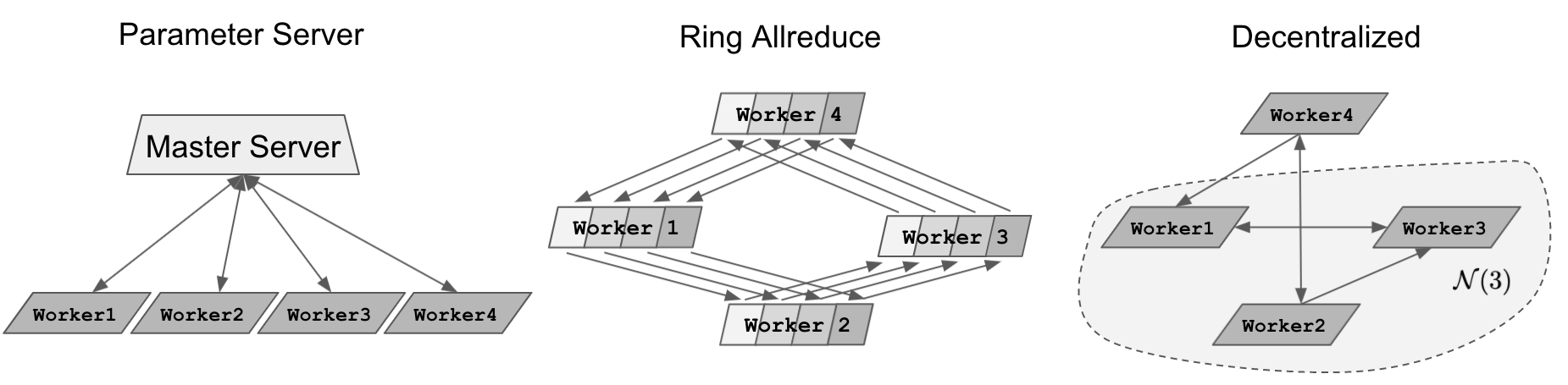
Figure 1: Illustration of Parameter Server, Ring-Allreduce, and decentralized partial averaging. In partial averaging, nodes exchange information over edges; nodes do not relay information. As an example, Node $3$ collects information from its neighbors $1$ and $2$. Other nodes do the same but not depicted.

It it worth mentioning there are natural networks (e.g., fish school) and man-created networks (e.g., transportation network), where controlling all the agents by a central leader is practically infeasible or prohibitively expensive [13, 14, 15, 16]. Decentralized algorithms are, therefore, fundamental methods for sensing, signal processing, and controlling in those networks.

We can write most known decentralized algorithms in a few lines of equations. However, realizing them in a computer network is quite complicated. In particular, implementing a set of coordinated communication steps between specific pairs of nodes requires a skillful application of low-level communication libraries. Therefore, despite the development of decentralized algorithms over the past two decades, we are yet to see a software package for their rapid implementations. Most decentralized algorithm developers have been simulating their algorithms on a single computer in Matlab or Python. The very few packages that can run in a computer network were written for specific algorithms and network topologies. Adapting them to another project requires modifying lower-level communication. The recent development further involves asynchrony, time-varying network topologies, and asymmetric communication have created an even higher implementation barrier.

We fill the gap between the rapid development of algorithms on paper and the lack of practice in real world with the introduction of BlueFog, a python library for straightforward, high-performance implementations of diverse decentralized algorithms.

1. Users with no experience with distributed systems can implement a decentralized algorithm in just a few clean lines of Python codes of a single program. The program will be run on multiple agents (with their different data) to achieve parallelism, which is commonly known as single program, multiple data (SPMD).

2. We design BlueFog to support a series of features for advanced users and future development. They include: the controls of partial-averaging coefficients, one-way communication in the pull and push forms, asynchrony, time-varying networks. We managed to keep the advanced communication primitives relatively simple through a unified abstraction of different decentralized communication operations.

3. BlueFog is designed to be used together with modern deep learning framework like PyTroch to train large deep neural networks. All features of these framework (e.g., network design, auto-differentiation, various optimizers) are unaffected.

4. We optimized BlueFog for efficient communication. BlueFog can be connected to a Message Passing Interface (MPI) library [17] for multi-CPU computing or the NVIDIA Collective Communications Library (NCCL) [18] for multi-GPU computing. On top of that, we implemented computation/communication overlapping, tensor fusion for multiple small tensors, hierarchical communication, and other acceleration techniques in BlueFog.

The BlueFog package comes with several examples as a tutorial. They include major decentralized algorithms for signal processing: decentralized gradient descent [19, 20], exact diffusion [21, 22], and gradient tracking [23, 24, 25, 26, 27]. We also include a deep-learning-based image classification example where BlueFog is $1.2\sim 1.8\times$ faster than Horovod [28], a state-of-the-art distributed training package based on Ring-Allreduce.

We comment on speed comparisons. Different distributed algorithms may return solutions in various manners. Those using a central agent typically form the solution at the central agent. In decentralized algorithms, all the agents converge to (nearly) the same solution uniformly; we take the solution at the rank-0 node. Comparing the performances of these two types of algorithms is not merely a task of comparing their costs-per-iteration (though we do in this paper) but also the numbers of iterations or total times for reaching a solution of the same accuracy. The theoretical analyses of iteration complexities and total running times are out of the scope of this paper; see [1, 3, 29, 30, 4, 5, 31] for some recent decentralized algorithms that are proven faster than distributed algorithms. This paper, however, provides some numerical comparison results that demonstrate BlueFog.

BlueFog is an open-source project that was first available on GitHub in December 2019. It keeps evolving during the past two years, and the progress was reported in some conferences. BlueFog has provided demos for several distributed and decentralized algorithms introduced in [32], and it has supported all deep learning experiments in [4, 5, 33]. All BlueFog code and supporting documents can be found at https://github.com/Bluefog-Lib.

I-A Organization

The rest of paper is organized as follows. Sec. II reviews decentralized optimization and algorithms. Sec. III provides a unified abstraction of the partial averaging operation that supports static or time-varying, push-style and pull-style, synchronous and asynchronous decentralized communication modes. Sec. IV illustrates the usage of BlueFog partial averaging with various applications in optimizations and signal processing. Sec. V highlights BlueFog’s system design that wraps the low-level decentralized communication primitives for providing state-of-the-art training performance for large-scale deep learning. Sec. VI discusses implementation details of BlueFog. The performance of BlueFog in deep learning training tasks are provided in Sec. VII. We conclude the paper in Sec. VIII.

II A Brief Review on Decentralized Optimization

II-A Concepts and Theoretical Foundations

This section gives a quick review of the components of decentralized optimization through the example of the decentralized (stochastic) gradient descent.

Problem. Partition a set of data $D$ to $n$ computing nodes, where node $i$ has access to local data $D_{i}$, $i=1,\dots,n$. Suppose they collaborate to solve the distributed optimization problem:

$${\color[rgb]{0,0,0}\min_{x\in\mathbb{R}^{d}}\ f(x)=\frac{1}{n}\sum_{i=1}^{n}f_{i}(x)\quad\mbox{where}\quad f_{i}(x):=\frac{1}{|D_{i}|}\sum_{\xi_{i}\in D_{i}}F(x;\xi_{i}).}$$ (1)

Node $i$ can evaluate stochastic gradient $\nabla F(x;\xi_{i})$, by sampling $\xi_{i}$ randomly, or compute the real gradient $\nabla f_{i}(x)$. We use stochastic gradient in the rest of this section.

Distributed method based on global averaging. Each agent independently computes $g_{i}^{(k)}=\nabla F(x_{i}^{(k)};\xi_{i}^{(k)})$, and they will synchronize across the entire network to achieve the globally averaged gradient to update $x$. This method can be described by the equations:

$$g_{i}^{(k)} =\nabla F(x_{i}^{(k)};\xi_{i}^{(k)}),\quad i=1,\dots,n$$ (local stochastic gradient) (2)

$$x^{(k+1)} =x^{(k)}-\frac{\gamma}{n}\sum_{i=1}^{n}g_{i}^{(k)}$$ (global averaging) (3)

where $\gamma$ is the stepsize or learning rate. The global averaging can be implemented via Parameter Server or Ring-Allreduce, see Fig. 1 for illustrations. Global averaging typically incurs significant communication overhead, which motivates the following decentralized approach.

Decentralized method based on partial averaging. In decentralized stochastic gradient descent [34, 20, 19], each agent computes a stochastic gradient, updates its local copy of $x$, and performs a partial averaging that involves the copies from its direct neighbors and itself. We can describe these steps by:

$$x_{i}^{(k+\frac{1}{2})} =x_{i}^{(k)}-\gamma\nabla F(x_{i}^{(k)};\xi_{i}^{(k)}),\quad i=1,\dots,n$$ (local update) (4)

$$x_{i}^{(k+1)} =w_{ii}x_{i}^{(k+\frac{1}{2})}+\sum_{j\in\mathcal{N}(i)}w_{ij}\,x_{j}^{(k+\frac{1}{2})},\quad i=1,\dots,n$$ (partial averaging) (5)

where $\mathcal{N}(i)$ is the set of neighbor agents of agent $i$ and the weights $w_{ij}$ are described below. The network topology and weights significantly affect the convergence performance and communication efficiency.

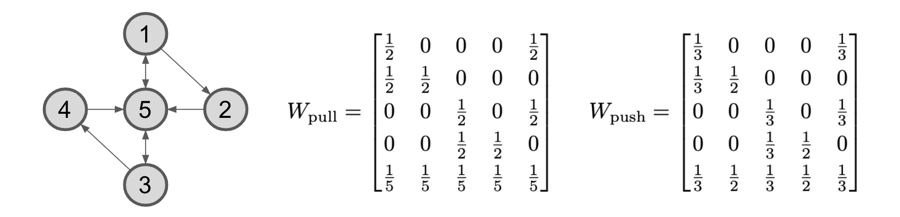
Figure 2: An example topology with 5 nodes and two possible associated weighted matrices (pull weight matrix $W_{\rm pull}$ in the middle and push weight matrix $W_{\rm push}$ in the right). Note the topology is directed and $W_{\rm push}$ are not the transpose of $W_{\rm pull}$.

Network topology. Consider a directed graph ${\mathcal{G}}=({\mathcal{V}},{\mathcal{E}})$, where ${\mathcal{V}}$ is the set of nodes and ${\mathcal{E}}$ is the set of directed edges. An edge $(i,j)\in{\mathcal{E}}$ implies that node $i$ can send information to node $j$. For each node $i$, define

$${\mathcal{N}}(i) =\{j:(j,i)\in{\mathcal{E}}\}\;\;\;\;\mbox{as its set of in-coming neighbors},$$ (6)

$${\mathcal{M}}(i) =\{j:(i,j)\in{\mathcal{E}}\}\;\;\;\;\mbox{as its set of out-going neighbors.}$$ (7)

Take node $5$ as an example in Fig. 2. It holds that ${\mathcal{N}}(5)=\{1,2,3,4\}$ and ${\mathcal{M}}(5)=\{1,3\}$.

Weight matrix. Given ${\mathcal{G}}$, define

$$w_{ij}\begin{cases}\in\mathbb{R}&\mbox{if $(j,i)\in{\mathcal{E}}$, or $i=j$}\\ =0&\mbox{otherwise.}\end{cases}$$ (8)

Weight $w_{ij}$ is applied to the copy of $x_{j}$ sent from node $j$ to node $i$ (notice the positions of $j$ and $i$ in the subscript); the weight is zero if node $j$ cannot send messages to node $i$. All weights form the matrix $W:=[w_{ij}]_{i,j=1}\in\mathbb{R}^{n\times n}$. Commonly-used weight matrix $W$ falls into one of the following three categories:

1. Pull matrix $W$ satisfies $W\mathds{1}=\mathds{1}$, i.e., every row adds up to $1$. Pull matrix $W$ is used with a directed graph.

2. Push matrix $W$ satisfies $\mathds{1}^{T}W=\mathds{1}^{T}$, i.e., each column of a push matrix $W$ adds up to $1$. Push matrix $W$ is also used with directed graph.

3. Standard weight matrix $W$ satisfies both $W\mathds{1}=\mathds{1}$ and $\mathds{1}^{T}W=\mathds{1}^{T}$ and used for undirected graph, as well as special directed graphs such as the exponential graph [33].

See Fig. 2 for examples of pull and push matrices. When $W\geq 0$, a pull matrix is also known as a row-stochastic matrix, a push matrix as a column-stochastic matrix, and a standard weight matrix as a doubly-stochastic matrix. There are lots of flexibility into the selection of $W$ to serve different needs.

Given $W$, we can also deduce a directed graph ${\mathcal{G}}=({\mathcal{V}},{\mathcal{E}})$ with ${\mathcal{V}}=\{1,\dots,n\}$ and ${\mathcal{E}}=\{(j,i):w_{ij}\neq 0\}$.

Communication efficiency. When the network topology is sparse (e.g., a ring or a one-peer exponential graph [3, 33]), each partial averaging step (5) incurs $O(1)$ latency and $O(1)$ transmission time (the inverse of bandwidth), which are independent of $n$. Since each node only synchronizes with its direct neighbors, there is low synchronization overhead. Table I compares the communication times of partial averaging and global averaging; see more discussions in Sec. II-B. It is observed that all global averaging primitives scale at $O(n)$, suffering from either a bandwidth-bound long delay or a long latency when $n$ is large.

TABLE I: Communication costs comparison [35]. $n$ is the number of nodes; $M$ is message size; $B$ is bandwidth; $L$ is latency of direct communication.

Comm. primitive	Comm. cost	Averaging type	Note
Parameter Server [11]	$\frac{nM}{B}+nL$	global averaging	require a central node
Ring-Allreduce [12]	$\frac{2M}{B}+2nL$	global averaging
Byte-PS [36]	$\frac{M}{B}+nL$	global averaging	require extra nodes
BlueFog, partial averaging	$\frac{M}{B}+L$	partial averaging

Iteration complexity. Iteration complexities, though unaffected by implementations, are essential properties of decentralized algorithms. We mention some recent results in passing. Although partial averaging alone is less effective in aggregating information than global averaging, some decentralized algorithms can match or exceed the performance of global-averaging-based distributed algorithms: [1, 29] established that decentralized SGD can achieve the same asymptotic linear speedup in convergence rate as (parameter server based) distributed SGD; [3, 33] used exponential graph topologies to realize both efficient communication and effective aggregation by partial averaging; [37, 38, 31, 39] improved the convergence rate of decentralized SGD by removing data heterogeneity between nodes; [40, 4, 30, 41] enhanced the effectiveness of partial averaging by periodically calling global averaging. BlueFog can implement all these algorithms including those use global averaging.

Brief history of decentralized optimization. Decentralized optimization can be traced back to [42]. Since then, it has been intensively studied in the control and signal processing communities. The first decentralized algorithms on general optimization problems include decentralized gradient descent [19], diffusion [34, 20, 43], and dual averaging [44]. Various primal-dual algorithms come out to further speed up the convergence, and they are based on alternating direction method of multipliers (ADMM) [45, 46], explicit bias-correction [47, 48, 49], gradient tracking [23, 24, 25, 26], and dual acceleration [50, 51]. In deep learning tasks, decentralize SGD also attracted a lot of attentions recently. Many efforts have been made to extend the algorithm to time-varying topologies [29], directed topologies [3, 27], asynchronous settings [2], and data-heterogeneous scenarios [52, 53, 31, 37, 38, 54, 39]. Techniques such as quantization/compression [55, 56, 57, 58, 59], periodic updates [60, 29, 61], and lazy communication [62, 63] were also integrated into decentralized SGD to improve communications.

II-B Related works

Libraries that support global averaging. Parameter Server (PS) [11] is a well-known architecture adopted early in TensorFlow [64] where all workers communicate with the central parameter server(s). It easily suffers from communication bottlenecks. If every worker sends a message of size $M$ to the central server and the network interface is saturated by every message, the total communication in PS is $n(\frac{M}{B}+L)$. Like PS, the Ring-Allreduce [12] architecture organizes all nodes on a ring and divides each local gradient tensor into $n$ chunks for parallel communication. Ring-Allreduce achieves a remarkable communication time of $\frac{2M}{B}+2nL$. The bandwidth-bound time $\frac{2M}{B}$ is optimal [65], where constant $2$ is not improvable (without hardware additions). Ring-Allreduce has been implemented in Horovod and Pytorch. Fig. 1 illustrates the Parameter Server and Ring-Allreduce operations. Another framework BytePS [36] is based on PS-lite [66] and can reduce the bandwidth cost from $\frac{2M}{B}$ to $\frac{M}{B}$ using $n$ additional CPU servers. Instead of passing each of the $n$ chunks over a ring, each worker pushes its $i$th chunk to server $i$ and pulls the accumulated chunk back, achieving a total communication time of $\frac{M}{B}+nL$. The communication overheads of Parameter Server, Ring-Allreduce, and BytePS are listed in Table I.

Libraries that support partial averaging. The open-source codes or libraries to provide the system-level partial averaging are limited. The codes brought along with [3, 67] implemented only the decentralized algorithms proposed therein. Prague [68] wraps all-reduce or broadcast operations, which is smart but relatively inefficient and restrictive. In particular, Prague forms a ring from a random subset of nodes and then ring-allreduces over them, thus ruling out other effective topologies such as the exponential graph [3, 33].

BAGUA [69] is a recent open-source library that supports both global and partial averaging, offers full- and low-precision operations, and focuses on efficient deep learning. It does not support asynchronous communication, diverse and time-varying network topologies, and directed communications in pull- and push styles, which are supported by BlueFog to implement algorithms such as push-sum [3] and push-pull [70, 71], as well as more recent decentralized algorithms using those features. BlueFog supports classic decentralized optimization and control with a tutorial that covers several examples, in addition to deep learning.

II-C Notation and Terminologies

BlueFog lies in the intersection between decentralized optimization and high-performance computation communities, so we use terms from both communities. Throughout the paper, we use process, node, and agent interchangeably. Each node has a unique ID called rank, a number starting from 0. The number of nodes is called the size of the graph. A super node refers to a physical machine, which may include one or more nodes inside. Most low-level communication primitives are named following the convention in MPI. We call the out-going and in-coming nodes as the destination and source nodes of that communication, respectively. Lastly, we use the terms topology, graph or network interchangeably to indicate how all nodes are connected.

III Abstraction of Decentralized Communication

Decentralized algorithms are diverse. For BlueFog to provide a clean and consistent interface, we begin with summarizing the major dimensions that describe the variations in how decentralized algorithms communicate:

1. Communicate over static or time-varying topology. The underlying topology in decentralized communication can remain static or keep changing over iterations.

2. Communicate in a push- or pull-style. The weight matrix associated with the topology can be push stochastic or pull stochastic; see Sec. II-A for the discussion on the weight matrix.

3. Communicate in a synchronous or asynchronous mode. Each node in decentralized communication can communicate and update information with or without synchronization with its neighbors.

An algorithm may include one or multiple of these features. For example, push-DIGing [25] uses synchronous communication in the push style over a time-varying topology. We develop primitives to support the above features, with more advanced primitives offer richer features and also require more inputs from the user.

The discussion in this section focuses on how we define and organized the programming interfaces, instead of their syntax, which we introduce in the next section with examples.

III-A Decentralized communication over static topology

We start with the primitives for the simplest case – synchronous communication over a static graph:

$${\mathcal{G}}=({\mathcal{V}},{\mathcal{E}})\;\;\;\;\mbox{(Global view)}$$ (9)

By global view, we mean the information of the graph, including all the nodes, edges, and weights, is made available to all the nodes. Once set up, ${\mathcal{G}}$ remain unchanged. The BlueFog primitive for this setup is:

$$\boxed{\mbox{set\_topology(graph\_object)}\to{\rm\;bool}}$$

where “graph_object” also contains the weight matrix $W$. BlueFog includes built-in implementation of commonly-used topologies including ring, grid, static exponential graph, and a few others. The user can create their own graphs with BlueFog.

After a graph is set up, each node can access the weights for its partial averaging. BlueFog provides the following collective communication primitive for partial averaging (5):

$$\boxed{\mbox{neighbor\_allreduce(tensor, name)}\to{\rm\;tensor}}$$

While partial averaging is a math term, its implementation neighbor allreduce follows the MPI naming convention, where reduce stands for reducing multiple tensors into one, all means all processes (nodes) are involved, and neighbor modifies “all” to include only the neighbors. Unlike allreduce, neighbor_allreduce returns different tensor values for different nodes in general as they may have different neighbors and use different weights. It is clearly not a stateless function.

III-B Push- and pull-style communication over time-varying topology

The primitives of last subsection cannot be applied to create time-varying graphs. We use a new primitive for time-varying graphs, which provides each node with a local view (e.g., the weights associated with its neighbors).

Another way to define decentralized communication is through the local view of each process (node). Recall the set of in-coming neighbors and out-going neighbors introduced in (6) and (7) are all local information associated with each node $i$. Knowledge of these two sets is sufficient to conduct partial averaging through local view. To this end, we extend partial averaging (5) to the time-varying topology as follows

$$x_{i}^{(k+1)}=w^{(k)}_{ii}x_{i}^{(k)}+\sum_{j\in{\mathcal{N}}(i)}r^{(k)}_{ij}s^{(k)}_{ij}x_{j}^{(k)}$$ (10)

where $r^{(k)}_{ij}\in[0,1]$ and $s^{(k)}_{ij}\in[0,1]$ both are the associated scaling weights when node $j$ sending the information to node $i$ at iteration $k$. Note that ‘$r$’ stands for receiving-side scaling and ‘$s$’ stands for sending-side scaling. If $r^{(k)}_{ij}s^{(k)}_{ij}=w_{ij}^{(k)}$ and $w_{ij}^{(k)}$ remains static for each iteration $k$, the recursion (10) reduces to the partial averaging step in (5). By introducing a dummy variable $y_{ij}$, the above partial averaging operation is equivalent to

$$y_{ij}^{(k)}=\; s_{ij}^{(k)}x_{j}^{(k)},\;\;i\in{\mathcal{M}}(j)\hskip 52.63777pt\mbox{(push-style communication)}$$ (11)

$$x_{i}^{(k+1)}=\; w^{(k)}_{ii}x_{i}^{(k)}+\sum_{j\in{\mathcal{N}}(i)}r_{ij}^{(k)}y_{ij}^{(k)}\hskip 28.45274pt\mbox{(pull-style communication)}$$ (12)

In the push-style communication (11), a sending node $j$ will scale its own variable $x_{j}^{(k)}$ with weight $s^{(k)}_{ij}$ to achieve $y^{(k)}_{ij}$, and push it to each of its out-going neighbor. In the pull-style communication (11), a receiving node $i$ will pull $y^{(k)}_{ij}$ from its in-coming neighbors and scales them with $r^{(k)}_{ij}$. Fig. 3 illustrates the push- and pull-style communications. Two circles are drawn around the sending node $j$ and receiving node $i$, respectively. The left circle illustrates the pull-style communication (11) while the right illustrates the push-style communication (12).

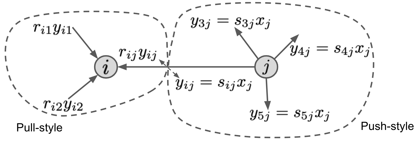
Figure 3: A illustration of the push- and pull-style communications. Node $i$ is pulling information from its in-coming neighbors while node $j$ is pushing information to its out-going neighbors. Note the pull-style circle and push-style circle are not necessary separable as plotted.

The introduction of the dummy variable $y_{ij}$ completely decoupled the pull-style communication with the push-style communication. A pure push-style partial averaging can be achieved by setting $r^{(k)}_{ij}=1$ and $s^{(k)}_{ij}=w^{(k)}_{ij}$. In addition, it is easy to guarantee $\sum_{i=1}^{n}s^{(k)}_{ij}=1$, i.e., utilize push weight matrix, since the weights $\{s_{ij}\}_{i=1}^{n}$ is determined by the sending node $j$. Similarly, a pule pull-style partial averaging can be achieved by setting $r^{(k)}_{ij}=w^{(k)}_{ij}$ and $s^{(k)}_{ij}=1$, and $\sum_{j=1}^{n}r^{(k)}_{ij}=1$, i.e., utilization of the pull weight matrix, can be easily guaranteed since the weights $\{r_{ij}\}_{j=1}^{n}$ is determined by the receiving node $j$. When $r^{(j)}_{ij}\neq 1$ and $s^{(j)}_{ij}\neq 1$, both push- and pull-style communications exist in partial averaging.

The neighbor_allreduce primitive provided in BlueFog supports (11) and (12) as follows

$$\boxed{\mbox{neighbor\_allreduce(tensor, name, [self\_weight, dst\_weights, src\_weights])}\to{\rm\;tensor}}$$

To be consistent with decentralized communication over static topology, we exploit the same function name but extend it with three more optional argument: self_weight, src_weights, and dst_weights. Here self_weight is simply a scalar corresponding to $w_{ii}$ for node $i$. In a local view of node $i$, src_weights stands for the weights $\{r_{ij}\}_{j=1}^{n}$ to scale tensors received from in-coming source nodes; similarly, dst_weights denotes $\{s_{ij}\}_{i=1}^{n}$ to scale tensors sent to out-going destination nodes. These three arguments enable partial averaging to be conducted with push-style, pull-style, or push-pull-style communication. In addition, the time-varying topology is now allowed since these three arguments can be passed to neighbor_allreduce per iteration. Fourthermore, the neighbor_allreduce primitive should also support automatic topology check (which is discussed in details in Section VI-C) to examine whether the weights specified by users are valid; otherwise the program may get stuck when the sending and receiving process do not match with each other.

III-C Asynchronous decentralized communication

Asynchronous decentralized communication is much more complicated than the synchronous one [2, 72, 35]. The key feature of asynchronous communication between processes is it decouples tensor movement with process synchronization. In other words, one process (node) is allowed to move tensors without synchronization with remote processes (i.e., the neighboring nodes).

This section proposes a solution inspired by the Remote Memory Access (RMA) technique [73, 74]. To enable asynchronous decentralized communication, each node (process) first registers a window, which is a memory chunk created for neighbors. A node can create multiple windows, and each window will be associated with a unique name and an immutable tensor. The total memory size of these windows is determined by the shape of the tensor as well as the number of in-coming neighbors. For example, if node 1 has two in-coming neighbors (say node 3 and node 5) and it owns a model parameter named “convolution.layer1.weights” with a shape of $5\times 5\times 3$, then it will register a continuous memory chunk capable to store a $150$-length vector ($150=5\times 5\times 3\times 2$), with the first half storing model “convolution.layer1.weights” received from node 3 and the remaining half from node 5. The following two primitives are developed in BlueFog for the window creation and deletion.

win_create(tensor, name) $$\to{\rm\;bool}$$

win_free(name) $$\to{\rm\;bool}$$

Note that topology is not specified in these primitives, and the global topology setting will be taken by default.

BlueFog next provides three communication primitives neighbor_win_put, neighbor_win_get and neighbor_win_accumulate (the names are borrowed from MPI protocol) to manipulate the remote memory. As their name indicate, neighbor_win_put puts local tensors to the window buffers maintained by its neighbors while neighbor_win_get fetches neighbors’ local tensors to its own local window buffers, see the illustration in Fig. 4. Primitive neighbor_win_accumulate performs similarly to neighbor_win_put, but the former adds local tensor to the existing window buffers maintained by its neighbor while the latter overwrites those buffers. During the window creation, we utilize static topology since frequently allocating and de-allocating windows are expensive. BlueFog provides the dst_weights and src_weights dictionary as arguments to the following three primitives to enable asynchronous data transferring defined over the dynamic topology. Note the window allocation is associated with the global static topology, which implies the ranks used in dst_weights and src_weights should be the subset of the neighbors defined under the global static topology.

neighbor_win_get(tensor, name, [src_weights]) $$\to{\rm\;bool}$$

neighbor_win_put(tensor, name, [self_weight, dst_weights]) $$\to{\rm\;bool}$$

neighbor_win_accumulate(tensor, name, [self_weight, dst_weights]) $$\to{\rm\;bool}$$

Note that these primitives support either dst_weights or src_weights but not both. Also, the put and accumulate primitive are suitable for push-style communication while the get one is for pull-style communication.

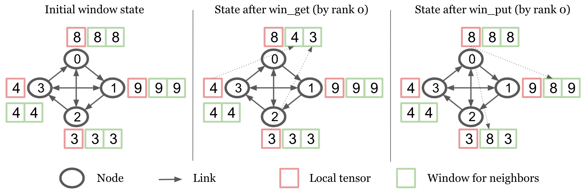
Figure 4: A illustration figure of win_put and win_get called by rank 0 (without any dst_weight or src_weight setting). In this example figure, the tensor is simply a scalar and each node has two in-coming neighbors.

These remote tensor transferring primitives alone are insufficient for asynchronous decentralized communication because 1) the local process does not know when the window buffer is updated and 2) above three communication primitives only transfer or manipulate the tensor within the window buffer, which is not the same tensor that used for local computation. As a result, one more primitive is provided in BlueFog to fill the gap – win_update. The functionality of win_update is in two-folds. First, it updates the buffer to ensure the tensors kept in window buffers, which may have be changed through neighbor_win_put, neighbor_win_get, or neighbor_win_accumulative, are synchronized and visible to local process. Second, it returns a tensor achieved by averaging the local and neighbors’ tensors.

$$\boxed{\mbox{win\_update(name, [self\_weight, src\_weights])}\to{\rm\;tensor}}$$

The behavior of win_update operation should return a weighted average tensor based on the local tensor and the latest tensor value from neighbors stored in the local window. We leave the usage of above asynchronous primitives in the asynchronous push-sum example in Sec. IV-C.

IV Application Examples

BlueFog implemented all previous mentioned communication primitives. Before explanation of implementation and the system design for deep learning usage, this section will first illustrate the usage of the decentralized communication primitives with examples in classical optimization.

IV-A Partial averaging over static graphs for linear regression

Decentralized linear regression. Suppose all nodes collaborate to solve the following linear regression problem

$$x^{\star}=\arg\min_{x\in\mathbb{R}^{d}}\quad\frac{1}{2n}\sum_{i=1}^{n}\|A_{i}x-b_{i}\|^{2}$$ (15)

where $A_{i}$ and $b_{i}$ are local data kept by node $i$. The target is to let each node $i$ achieve the optimal solution $x^{\star}$.

Decentralized gradient descent. Decentralized gradient descent (DGD) is among the most widely-used approaches to solving problem (15). In particular, DGD with static graph topology will iterate as follows:

$$x_{i}^{(k+\frac{1}{2})} =x_{i}^{(k)}-\gamma A_{i}^{T}(A_{i}x_{i}^{(k)}-b_{i})\hskip 56.9055pt\mbox{(local update)}$$ (16)

$$x_{i}^{(k+1)} =w_{ii}x_{i}^{(k+\frac{1}{2})}+\sum_{j\in{\mathcal{N}}(i)}w_{ij}x_{j}^{(k+\frac{1}{2})}\hskip 36.98866pt\mbox{(partial averaging)}$$ (17)

where ${\mathcal{N}}(i)$ is the in-coming neighbors of node $i$.

Code. We set the topology as the static exponential graph in the following DGD implementation, which is established in [33] to be both sparse and well-connected. Note that such static exponential graph and its associated weight matrix $W$ has already been implemented in the BlueFog library. Users can directly set it as the default topology over which DGD runs. The code snippet of the DGD implementation using BlueFog is shown in Listing 1. The complete code can be referred to BlueFog online tutorial. It is observed that the DGD implementation using BlueFog is pretty strait-forward; the code is basically the python interpretation of the math equation (16)–(17). In addition to the exponential graph, many other directed or undirected static topologies have also been implemented in BlueFog such as ring, star, mesh, and fully-connected topology. Users can also set up their own topology in BlueFog to facilate decentralized algorithms.

⬇

1import bluefog.torch as bf

2bf.init() # Initialize the BlueFog

3

4# Set topology as static exponential graph.

5G = bf.ExponentialTwoGraph(bf.size())

6bf.set_topology(G)

7

8# DGD implementation

9for ite in range(maxite):

10 grad_local = A.t().mm(A.mm(x) - b) # compute local grad

11 y = x - gamma * grad_local # local update

12 x = bf.neighbor_allreduce(y) # partial averaging

Listing 1: BlueFog implmentation of the DGD algorithm to solve decentralized linear regression.

Other well-known algorithms such as Exact-Diffusion and Gradient-Tracking to solve problem (15) over static undirected or time-varying directed topology are implemented using BlueFog in Appendix -A and -B.

IV-B Partial averaging over time-varying graphs

Mobile adaptive networks. Mobile adaptive networks are classical applications of decentralized optimization over networks. A typical example of mobile adaptive network is the fish schools. While each single fish has limited abilities, the fish schools can exhibit sophisticated behavior that arises from interactions among adjacent members of the school. When a predator is sighted or sensed, the entire school of fish adjusts its configuration to disperse. The fish schools can even encircle or attack the predator with remarkable disciplines.

In this subsection, we simulate the above behaviour of fish schools with BlueFog. We mimic each fish with one process in a CPU cluster. With the system-level neighbor-allreduce, neighbor-allgather, and the topology-oriented APIs provided by BlueFog, we can easily schedule the time-varying fish topology, recognize the dynamic neighborhood, and conduct local information exchange between neighboring fishes. Note that the topology of fish schools is highly dynamic especially when fishes are escaping or encircling, this simulation will test how robust BlueFog is to dynamic topology scheduling.

Problem formulation. Consider $n$ fishes distributed over some spatial region. Two fishes are said to be neighbors if they are within a predefined distance. The objective of the fish school is to estimate the predator’s location in a fully decentralized manner and take actions such as disperse or encircle. The estimation of the predator’s location can be formulated into a distributed optimization problem. For fish $i$ at time $k$, it will have a local estimate of the distance $d_{i}^{(k)}$ and the azimuth angle $\theta_{i}^{(k)}$ between the predator and itself. If we denote the direction vector as $u_{i}^{(k)}=[\cos\theta_{i}^{(k)}\ \sin\theta_{i}^{(k)}]^{T}\in\mathbb{R}^{2}$, the relation between distance $d_{i}^{(k)}$, the fish’s current position $x_{i}^{(k)}$, and the predator’s position $w^{\star}$ can be characterized as $d_{i}^{(k)}=(u_{i}^{(k)})^{T}(x_{i}^{(k)}-w^{\star})+n_{i}^{(k)}$, where $n_{i}^{(k)}$ denotes additive noise. If we let $f_{i}(w)=\frac{1}{2}[d_{i}-u_{i}^{T}(x_{i}-w)]^{2}$ to be the local loss function of fish $i$ to estimate the predator’s position $w^{\star}$, the global loss function of the fish schools to estimate the predator’s position can be formulated as $w^{\star}=\arg\min_{w}\{\sum_{i=1}^{n}f_{i}(w)\}$, which is a distributed optimization problem and can be solved with decentralized stochastic gradient descent (4) and (5). When $w_{i}^{(k+1)}$ is estimated at time $k$, each fish will either escape from the predator or encircle it at time $k+1$. The detail to formulate these fish behaviors can be referred to [75].

Code. The simulation of fish schools with BlueFog is to illustrate how to use partial averaging over time-varying graphs. The code snippet is shown in Listing 2. Note the neighborhood at each iteration is determined by the argument src_weights, which is a dictionary mapping the rank to the scaling weights. The argument src_weights is updated at each iteration through the neighbor location collections function and Metropolis-Hastings Rule.

⬇

# x: self location; v: self velocity; w: predator location;

for k in range(maxite):

...

nb_ranks, nb_degrees = get_neighbor_ranks(x, loc_map, threshold)

# Set topology weights according to Metropolis-Hastings Rule.

self_weight, src_weights = get_mh_weights(nb_ranks, nb_degrees, bf.rank())

# observe noisy dist and direct to predator

# w_star is a predefined predator’s position

# w_star can change with time

d, u = get_dist_and_direct(x, w_star)

# estimate predator’s position w with D-SGD

grad = cal_grad(x, w, d, u)

w = w - gamma * grad

# Pull-style neighbor communication

w = bf.neighbor_allreduce(x, self_weight=self_weight, src_weights=src_weights)

# take escape or encircle actions

# location and velocity will get changed

if escap_cond:

x, v = escape(x, v, w)

elif encircle_cond:

x, v = encircle(x, v, w)

Listing 2: Code snippet to simulate school fishes

Simulation results. Figs. 5 and 6 depict how the fish schools disperse from and encircle a predator, respectively. These two figures illustrate that BlueFog is very effective to conduct partial averaging over dynamic topologies.

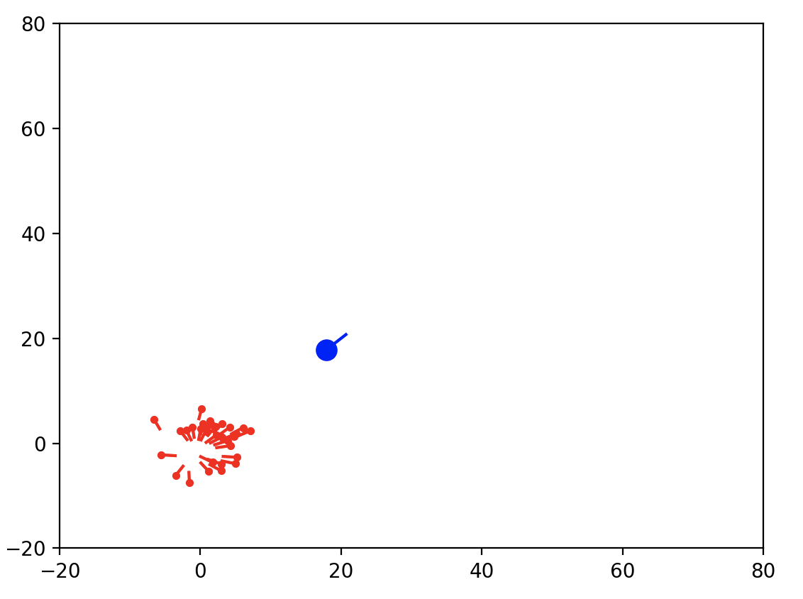
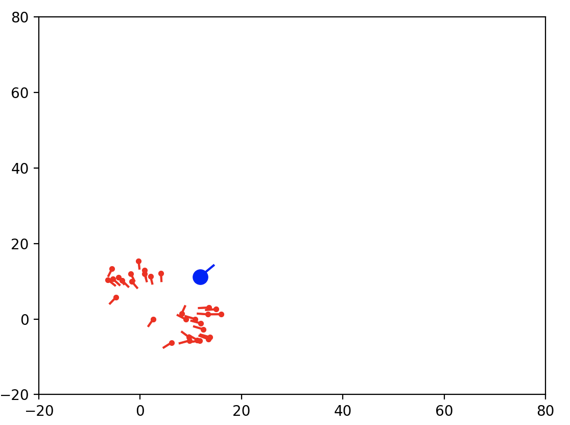
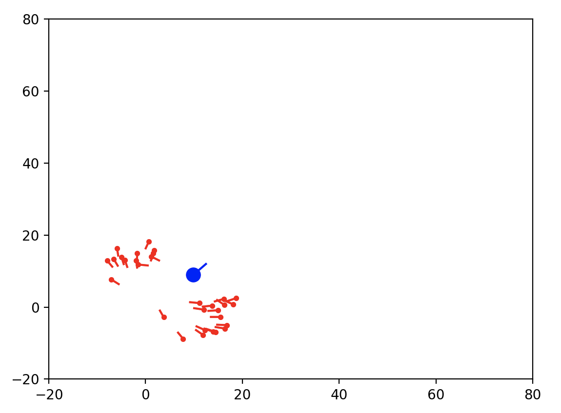
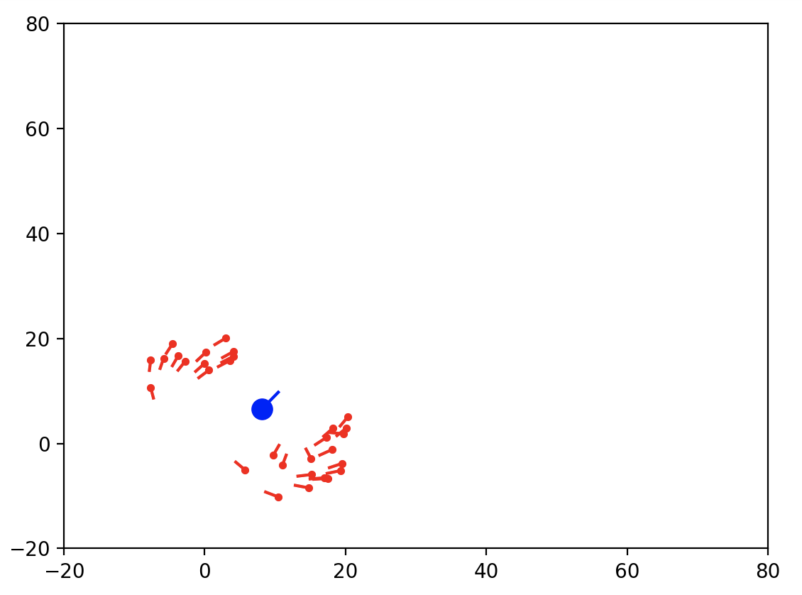
Figure 5: The fish schools dispersed when encountering a predator.

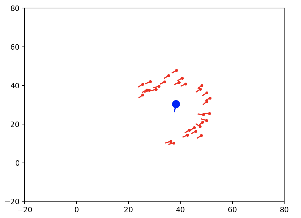
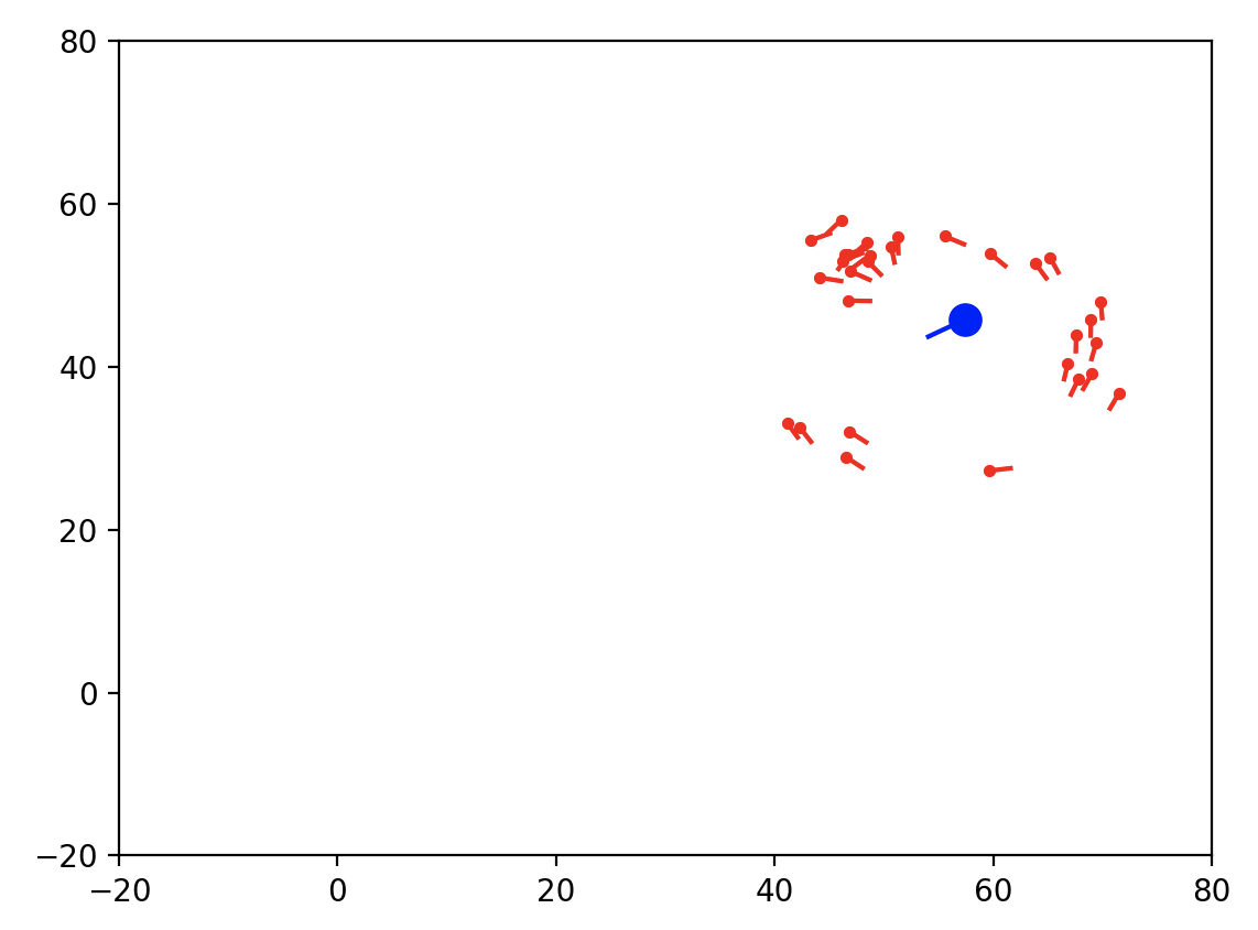
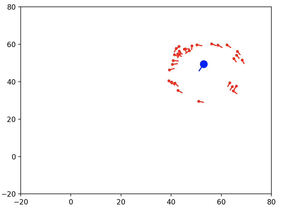
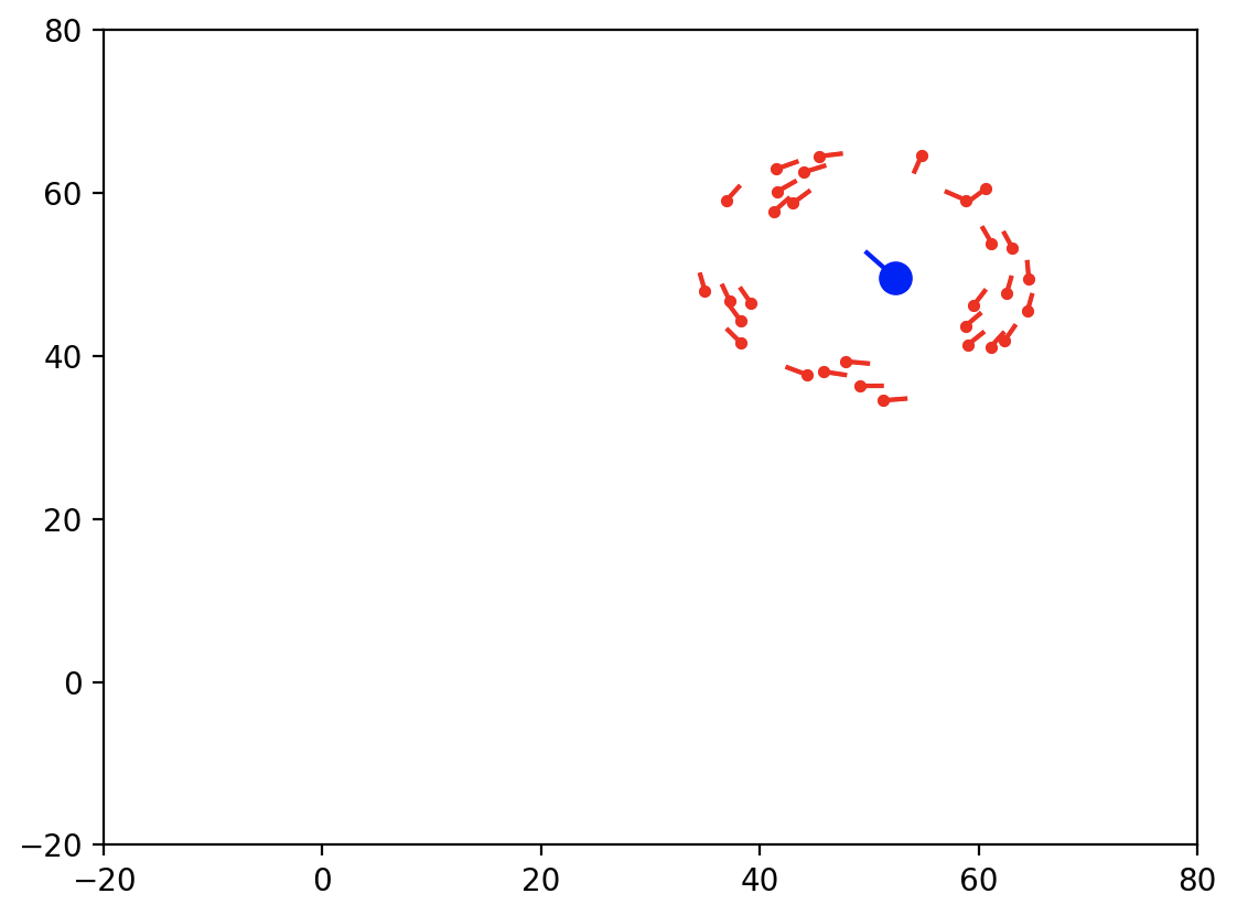
Figure 6: The fish schools encircled and trapped the predator.

IV-C Asynchronous push-style partial averaging

Average consensus problem. This subsection will provide an example on how to use asynchronous push-style primitives. Due to the complexity of asynchronous operations, we only consider the simple average consensus problem for illustration. Suppose every agent $i\in{\mathcal{V}}$ has a vector $x^{(0)}_{i}$. The goal is for all the agents to obtain the average

$$x^{\star}=\frac{1}{n}\left(x^{(0)}_{1}+x^{(0)}_{2}+\dots+x^{(0)}_{n}\right).$$ (18)

Since the channel between each pair of connected nodes may vary drastically in communication efficiency, it is possible that some node will finish the partial averaging earlier than the others. Asynchronous average consensus algorithm is proposed to avoid idleness in the fast node when it waits for the slow nodes.

Asynchronous push-sum average consensus algorithm. The vanilla asynchronous average consensus algorithm will result in a biased average for each node. To remove the bias, the push-sum asynchronous algorithm is proposed:

$$x^{(k)}_{i}= w_{ii}x^{(k-1)}_{i}+\sum_{j\in{\mathcal{N}}(i)}w_{ij}x^{(k-\delta_{j})}_{j}$$ (19)

$$p^{(k)}_{i}= w_{ii}p^{(kt-1)}_{i}+\sum_{j\in{\mathcal{N}}(i)}w_{ij}p^{(k-\delta_{j})}_{j}$$ (20)

$$y^{(k)}_{i}= x^{(t)}_{i}/p^{(k)}_{i}$$ (21)

where $p_{i}$ is a scalar correct $x_{i}$ and is initialized as value 1, and $\delta_{j}$ stands for some index difference since there is no global synchronized index in the asynchronous setting. When the weight matrix $W=[w_{ij}]$ is column stochastic, i.e. $\sum_{i}w_{ij}=1$, it is proved in [76, 77] that each $y^{(k)}_{i}$ will converge to the unbiased consensus value $x^{\star}$. For this reason, we will utilize the asynchronous primitives provided by BlueFog in the push-style.

Code. The following code snippet is to illustrate how to use partial averaging in the asynchronous and push-style mode. The complete code and experimental results can be referred to BlueFog online tutorial.

⬇

1p = torch.DoubleTensor([1.0]).to(x.device) # associated p for correction

2x_ext = torch.cat([x, p], 0)

3bf.win_create(x_ext, name="x_ext", zero_init=True)

4

5# Set up the weights through the push-style.

6outdegree = len(bf.out_neighbor_ranks())

7dst_weights = {rank: 1.0 / (outdegree + 1) for rank in bf.out_neighbor_ranks()}

8self_weight = 1/(1+outdegree)

9

10for i in range(args.max_iters):

11 bf.win_accumulate(x_ext, name="x_ext", self_weight=self_weight,

12 dst_weights=dst_weights, require_mutex=True)

13 bf.win_update_then_collect(name="x_ext")

14 x, associated_p = x_ext[:-1], x_ext[-1]

15

16bf.barrier() # Because different processes may end in different time.

17bf.win_update_then_collect(name="x_ext")

18bf.win_free(name="x_ext")

Listing 3: Example of using asynchronous primitives to implement the push-sum algorithm.

Remark. There are a few details in Listing 3 that we do not discuss in the previous sections. First, we add a new argument require_mutex=True in bf.win_accumulate. Such mutex is to guarantee the memeory read and manipulation operations will not be conducted at the same time, which is crucial to avoid the date race problem since two process do not synchronize with each other. Second, we use win_update_then_collect instead of win_update. The former operation will reset the window memory, i.e. setting all the elements in the window to be zero, after reading it. This operation needs to be atomic so that the sum of $p_{i}^{(k_{i})}$ (the sum of the value in the local tensor and the corresponding windows) over all agents is guaranteed to remain as the initial value in all iterations.

V System Design

Besides the low-level communication primitives discussed previously, more system-level design is required to construct a powerful framework supporting generic decentralized training with great performance. In this section, we will discuss what extra system-level components and optimizations we deploy enables BlueFog to achieve the state-of-the-art performance for large-scale deep neural network training tasks.

The design philosophy for these high-level APIs shift a little from these low-level communication primitives. The later ones expose many but universal control knobs out so that the user can have full freedom and capability to design various decentralized algorithms. In contrast, we make high-level APIs concise and easy-to-use to support a few off-the-shelf high performance decentralized optimization solutions. But we still leave users the whole control over topology choices which can applied on any generic decentralized algorithm.

First, we provide an example of using BlueFog for a deep neural network training task:

⬇

1import torch

2import bluefog.torch as bf

3# initialization and model and data settings.

4...

5opt = optim.SGD(model.parameters(), lr=0.01)

6# BlueFog wraps the standard optimizer to use the decentralized communication

7# to fuse the information with neighbors.

8opt = bf.DistributedAdaptThenCombineOptimizer(

9 optimizer=opt,

10 model=model,

11 communication_type=CommunicationType.neighbor_allreduce)

12for batch_idx, (data, target) in enumerate(train_loader):

13 ...

14 # Generate dynamic topology weights

15 opt.self_weights = self_weights

16 opt.src_weights = src_weights

17 opt.enable_topo_check = True

18 # Periodic global allreduce

19 opt.communication_type = CommunicationType.allreduce if batch_idx % 20 == 0

20 else CommunicationType.neighbor_allreduce

21 # Forward and backward computation.

22 output = model(data)

23 loss = F.cross_entropy(output, target)

24 loss.backward()

25 opt.step()

26 ...

Listing 4: Example of using distributed optimizer wrapper. The topology information is passed down to optimizer through external control. In the example, it also periodically runs global allreduce every 20 iterations.

In the code snippet above, we omit most initialization, model, and data setting. This is because the BlueFog optimizer should be non-intrusive by design and all parts unrelated to the optimizer should remain the same as the standard distributed training code. Basically, what the user need to do is just to wrap the standard optimizer with the BlueFog API, transforming the original optimizer into a decentralized one. As seen in the above example, the wrapped optimizer also accepts the arguments like src_weights, communication_types, etc, to configure the communication to be executed at each iteration. These settings should be placed before the forward and backward computation because the communication may trigger during the forward propagation, the backward propagation, or the step function, depended on what kind of decentralized optimizer is used. Next, we delve into a few key components that BlueFog adopts under these high-level APIs.

V-A Overlapping communication and computation

Typically, both communication and computation are time-consuming resource-intensive operations. The communication operations are mainly handled by network interface cards (NICs) and the communication overhead mostly comes from waiting the information sending to / received from other processes, while most (forward or backward propagation) computation operations happen on the CPU/GPU. These two types of operations by nature are independent, so ideally, executing communication and computation in parallel whenever possible is a good strategy to reduce overhead and make full use of system resources, which is also the key to gain more linear scaling speedup in the decentralized learning scenario.

Here, we first focus on the low-level primitives, which allows users not only to design various decentralized algorithms freely but also to easily write programs enjoying great performance boost by parallelism. In the later sub-section, we will show how we integrated this notion into the decentralized optimization algorithm to provide system level optimization.

To empower this idea, we support the non-blocking version of neighbor_allreduce primitives. The nonblocking version shares the same input arguments with the blocking counterpart, but they differ in what they return. The blocking one wait until the communication is finished then returned the combined tensor, which obviously doesn’t allow the user to overlap it with computation. The nonblocking one, instead, returns a handle (basically an unique integer) to identify the communication request. Because the nonblocking API doesn’t need to wait for other nodes to finish communication, it can return the handle immediately. Behind the scene, BlueFog system transfers the handle to a separate thread dedicated for communication. Hence, the user can write other computation routine after the nonblocking API. When the results of communication are required, an extra bf.wait() API, taking the previous returned handle as input, should be called. It mainly synchronize with other nodes to ensure the communication finishes, returning a reduced tensor as output. The following Listing 5 illustrates the usage of non-blocking operation.

⬇

1handle = bf.neighbor_allreduce_nonblocking(x, self_weight, src_weights, dst_weights)

2grad = ComputeGradient(x) # Communication in parallel

3# Wait() returns the tensor until the communication is done

4x = bf.wait(handle) - lr * grad

Listing 5: Example of using nonblocking function to overlapping the communciation and computation.

As for the asynchronous operations, like neighbor_win_put, neighbor_win_get, etc, they also have their corresponding nonblocking version of APIs. Note that asynchronous and nonblocking are two orthogonal concepts here. The former is defined between the two separated nodes or processes and the later is defined within the local node between communication and computation threads.

V-B Enabling hierarchical communication

Previously, we only consider the ideal case where each node is equivalent to each other; the nodes are isotropic in terms of placement; the bandwidth between each node pair is the same. However, it is extremely difficult to have a practical system perfectly align to these ideal conditions. Here we mainly consider one case that the bandwidth and placement of GPUs are different. Take DGX-1 for instance[78]. Its intra-machine communication between GPUs uses high-speed NV-Links, while its inter-machine communication uses slower NICs. Multiple rounds of intra-machine communication may take the same or even less time than a single inter-machine one. This implies that we should minimize the inter-machine communication as long as it does not change the functionality,

Hence, BlueFog introduces another API hierarchical_neighbor_allreduce for networks with two tiers of communication speeds, which contain multiple super nodes (machines) benefiting from faster intra-machine communication. See Fig. 8 as an example. Its execution can be divided into three stages. Firstly, within the same machine, all local nodes communicate with each other and formulate a local averaged tensor to represent the result from the machine. Then, the super node (a particular local node inside the machine) talks with the machine neighbor to compute the neighborhood averaging. Lastly, all the local nodes within the machine set the neighbor averaged value from machine level communication as its local averaging result.

Unlike the hierarchical version of allreduce operator, which shares the same functionality but just different implementations with non-hierarchical one, the hierarchical_neighbor_allreduce is no longer equivalent to its non-hierarchical counterpart in terms of functionality. Mainly, it is because the topology and the corresponding neighborhood definition are based on the super-node (machine) level instead of local node (process rank) level. Under a homogeneous environment, i.e. the number of nodes inside each machine is the same, the translation between node rank and machine rank is easy as follows:

$${\rm machine\_rank}= {\rm rank\;//\;local\_size},\;\;\;\;\;{\rm rank}={\rm machine\_rank*local\_size+local\_rank}$$

where $//$ means the integer division and local_rank and local_size represent the rank and size of processes inside one physical machine/super node, respectively. The behavior of the hierarchical API is ill-defined when difference machines have different number of processes. So, we don’t recommend the usage of this API under this situation. In summary, we have these two new corresponding APIs

$$\boxed{\mbox{set\_machine\_topology(graph\_object)}\to{\rm\;bool}}$$

$$\boxed{\mbox{hierarchical\_neighbor\_allreduce(tensor, name, [self\_weight, src\_machine\_weights, dst\_machine\_weights])}\!\to\!{\rm\;bool}}$$

Note we adopted the same style as neighbor_allreduce except adding keyword ‘machine’ to the arguments. Be default, the machine rank that each process or node belongs to is automatically detected by the program.

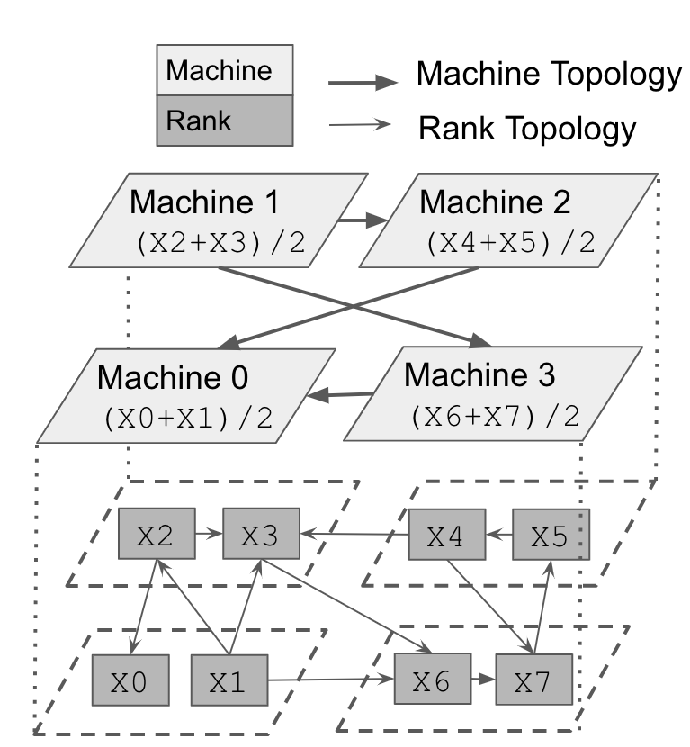
Figure 7: The illustration of hierarchical_neighbor_allreduce. In this example, each machine own two processes and $Xk$ represents the input tensor at rank $k$.

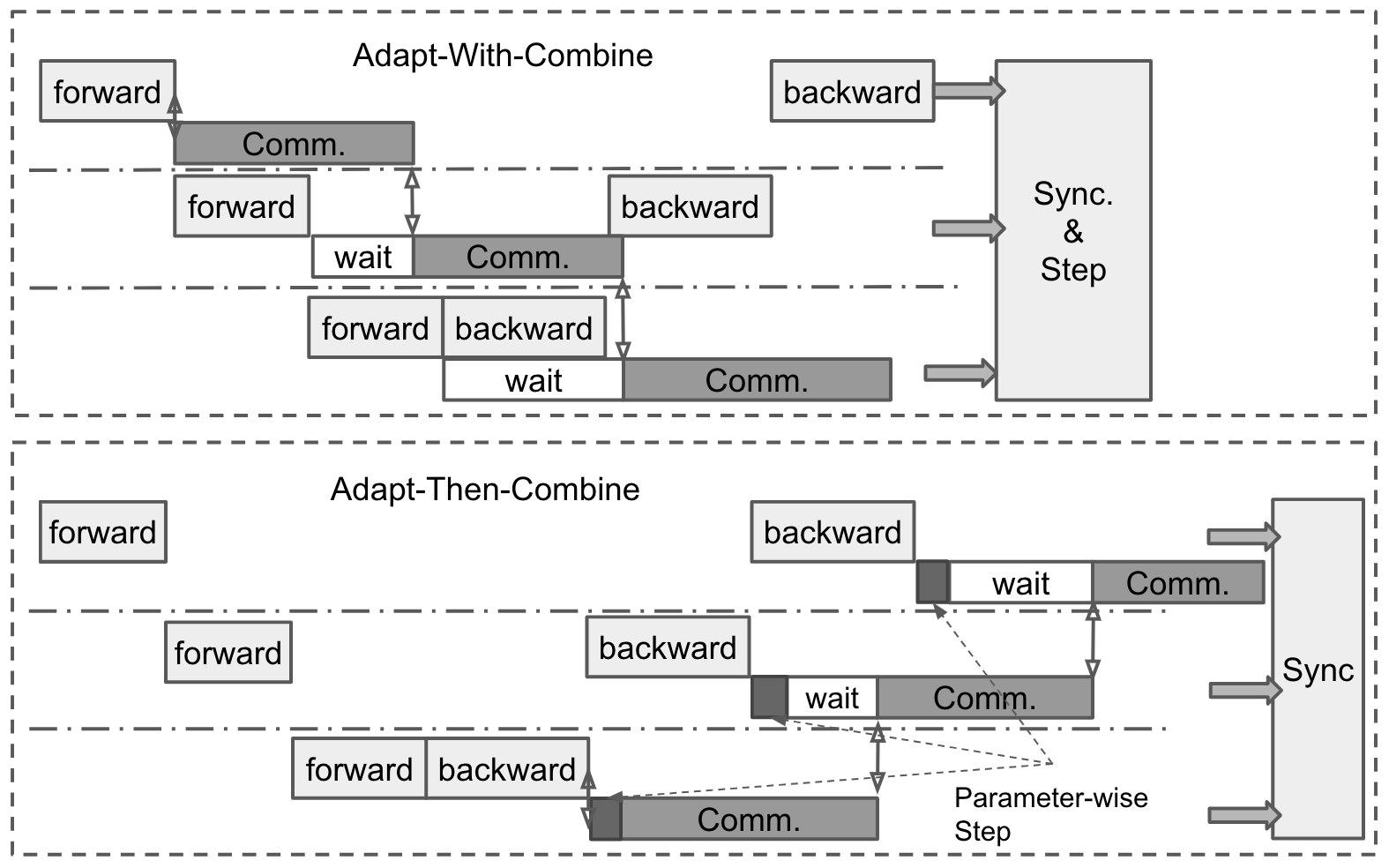
Figure 8: A timeline illustration of AWC and ATC algorithm over a three-layer neural network. Note this is an illustration for the toy example without other optimization techniques. In practice, due the tensor fusions and negation between the nodes, the pattern may vary.

V-C Triggering communication in deep learning optimizers

With the nonblocking APIs discussed in Section V-A, we are able to overlap the time for communication and computation. Obviously, more time we can overlap between them, better linear speedup we can get when the network size scales up. In consequence, we should trigger the communication as early as possible. Typically, the decentralized algorithms have at least two variants in terms of the execution order between communication and computation. In contrast, the allreduce based algorithm is always triggered after gradients are computed by the backward propagation. Using the Decentralized SGD algorithm as example, we have the following two variants:

$$x_{i}^{(k)}= \overbrace{\sum_{j\in{\mathcal{N}}^{\dagger}(i)}w_{ij}x_{j}^{(k-1)}}^{\rm Communication}-\gamma\overbrace{\nabla F(x_{i}^{(k)};{\boldsymbol{\xi}}_{i}^{k+1})}^{\rm Computation} {\rm(AWC\ style)}$$ (22)

$$x_{i}^{(k)}= \underbrace{\sum_{j\in{\mathcal{N}}^{\dagger}(i)}w_{ij}\left(x_{j}^{(k-1)}-\gamma\underbrace{\nabla F(x_{i}^{(k)};{\boldsymbol{\xi}}_{i}^{k+1})}_{\rm Computation}\right)}_{\rm Communication} {\rm(ATC\ style)}$$ (23)

We call (22) as Adapt-While-Communicate (AWC) style algorithm and call (23) as Adapt-Then-Communicate (ATC) style algorithm. As their names indicated, AWC algorithm can perfectly perform the computation and communication in parallel while ATC algorithm have to communicate after the computation is done. The situation is slightly more complicated if we apply these two algorithm variants on the deep neural network (DNN) training since gradient computation for DNN is layer-wise [79, 80]. This layer-wise computation nature implies that we can execute the communication of partial parameters (commonly the parameters in one layer) when all pre-requisition computation is done. This is crucial because even for the ATC-style algorithm (23) although the communication has to wait until the gradient is computed, we can still overlap the communication of one layer with the computation of the next layer. Consider a concrete example of applying (22) and (23) on a toy three-layer neural network, of which the timeline is illustrated in Fig. 8. In deep learning frameworks like PyTorch, it provides the hook that can register the function to be triggered when the forward computation or backward propagation of a layer is finished. In the figure, we can see that we register the communication for the AWC-style algorithm when the forward computation is done since it can maximize the overlapping; while it is not possible for the ATC-style algorithm but we can still register it under the backward one. Moreover, it is not hard to deduce that the deeper the neural network is, the larger portion the communication in ATC-style algorithm may overlap with its computation. Here we discussed the optimizers corresponding to ATC- and AWC-style. Actually, BlueFog provides more off-the-shelf high-level APIs for different styles of optimizers. Please refer to the BlueFog documentation website for more information.

V-D Miscellaneous system components

There are more system components that BlueFog implements for extra functionalities or performance boost such as tensor fusion for the merging multiple small tensor together, difference scaling strategies for the push-style and pull-style settings, timeline function to analysis the usage of each operation, the distributed mutex implementation for the window primitives, tolerating different orders of gradients or parameters triggered in different agents, etc. Since BlueFog already provides several wrapped decentralized optimizers off-the-shelf, most users do not need to know these low-level details. If the user want to implement his/her own decentralized algorithm, mainly they just need to focus on what communication primitives to use and when and how to overlap the communication and computations. After these design decisions are made, the user can refer to our preset optimizers and create his/her own optimizer.

VI Implementation

Figure 9: BlueFog’s architecture.

BlueFog fully integrates with the PyTorch library [81] so that the BlueFog APIs can be easily called in Python for decentralized tensor/vector computation and the core communication logic is implemented in C++ for better efficiency and faster interaction with low-level communication libraries like OpenMPI and NCCL. It is easy to install BlueFog by simply running pip install bluefog.

VI-A Architecture Overview

BlueFog architecture is composed of an application layer and a system layer. The former implements the low-level APIs and the optimizer wrapper described in Section III and Section V. The latter is dedicated to the underneath actual communication protocol in the system. Fig. 9 provides an overview of the entire architecture.

The application layer consists of three types of APIs: 1) topology management APIs such as set_topology and set_machine_topology; 2) low-level communication APIs such as allreduce, neighbor_allreduce, neighbor_win_get, etc.; 3) high-level distributed optimizer wrappers. In addition, BlueFog provides bfrun, a thin wrapper over mpirun to initiate BlueFog processes, and ibfrun to use BlueFog in interactive python environment such as Jupyter Notebook.

The system layer consists of two threads. The main thread, created by Python, is responsible for computation and generating communication requests. After the communication API like neighbor_allreduce is called by application layer, BlueFog transforms them into a proper request structure and push that into the shared queue. The application layer will then receive the handle of the enqueued request for fetching results in the future. Another thread is dedicated to communication, necessary for the nonblocking routine implementation. It pops out the requests from the shared queue, and then negotiates the requests with other BlueFog processes to schedule the communication order, which will be discussed more in Section VI-C. When all processes are ready, the negotiation service will inform the execution service to exchange the tensor information between processes.

VI-B Implementation of Low-level Primitives

BlueFog implements the neighbor_allreduce and hierarchical_neighbor_allreduce on both MPI and NCCL. Unless specified through the environment variables, BlueFog automatically chooses the underlying communication library. If the tensor is on CPU, MPI takes the responsibility of communication. If the tensor is on GPU, NCCL is used.

Figure 10: An illustration Dataflow of Hierarchical Neighbor Allreduce of 4 GPUs in one machine. 1. Intra-machine allreduce over NV-Links. 2. Inter-machine neighborhood communication through NIC. Here we skipped the CPU for simplicity. It may need CPU involvement if it running with TCP or without running with RDMA 3. Intra-machine Broadcast of received neighbor information.

MPI as backend

Although only a single synchronous neighborhood communication API is used for both static and dynamic topology usage, the implementation for them is different underneath.

For the static topology, BlueFog relies on neighborhood collective operations, which are added in MPI-3 standard [82, 74, 73]. Among them, the MPI_Neighbor_allgatherv API fits our requirements. Roughly, we can build the graph communicator for the provided global static topology. Then, neighbor information is collected through the MPI_Neighbor_allgatherv routine. Lastly, the weighted average over received information will generate the final neighbor_allreduce result, where the weights can be specified by the self_weight, src_weights, and dst_weights arguments. The advantage of using the native MPI routine is that MPI vendor may optimize the transmission order in the graph to avoid the traffic conflict as much as possible.

But this approach is not ideal for the dynamic topology. Creating graph communicators for all possible dynamic topology is expensive. Managing and associating the topology with the graph communicator is difficult because matching two dynamic graphs can be inefficient. Hence, the peer-to-peer communication is used to replace MPI_Neighbor_allgatherv. The destinations and sources of peer-to-peer communication are established on-the-fly through the src_weights and dst_weights arguments provided by users. To alleviate the communication congestion that multiple processes send to the same destination, the destination order at each process is sorted based on the difference between its own rank and the destination rank.

To implement hierarchical_neighbor_allreduce, it is slightly different from the previous implementation for neighbor_allreduce. It roughly takes four steps: 1) Intra-machine allreduce (SUM); 2) Inter-machine neighborhood communication; 3) Intra-machine broadcast; 4) Reduce the received tensor locally. The inter-machine communication is always executed by local rank 0 in each machine. To achieve inter- and intra-machine communication, two more communicators are built. One is a local communicator that connects all the processes in one machine and another is a global communicator that connects all processes with local rank 0. For static and dynamic machine topology usage, the inter-machine communication is the similar as neighbor_allreduce mentioned before.

The asynchronous primitives’ implementation is based on the window operations provided after MPI-3 standard. Internally, we maintain a state dictionary that maps from the unique window name to the registered window object. Each window object is also associated with a distributed mutex that can be locked and unlocked by the local process and the corresponding neighbor process. Since each window object may associate with multiple neighbors, each data manipulation primitive will automatically calculate the displacement value for the remote window based on the tensor shape and the rank.

NCCL as backend

NCCL implementation depends on the NCCL version. Before the NCCL 2.7 version [18], it only provides the collective communications – allreduce/broadcast/allgather, etc. In order to implement neighbor_allreduce, we have to create multiple pair communicators and then use broadcast under each pair communicator to mimic the send and receive operations. To avoid potential dead-lock problems, we sort the order of pair communicators first to align the send/receive usage among different processes. Each pair communicator is uniquely identified by the source and destination ranks, which are used to determine the order. Fortunately, NCCL provides the peer-to-peer communications since version 2.7. New ncclSend and ncclRecv APIs are introduced [18], which enables more efficient implementation and boosts our performance as well. We use the group functions ncclGroupStart and ncclGroupStop merging multiple peer-to-peer communications to form the neighborhood communication. Using these group functions, the deadlock problem is completely handled by NCCL.

As for hierarchical_neighbor_allreduce, NCCL’s implementation is similar as the MPI case, which also takes the same four steps. The advantage of using hierarchical_neighbor_allreduce over GPU is because it can fully exploit the high-speed NVLink that has been optimized for allreduce operation. An illustration dataflow of hierarchical_neighbor_allreduce of 4 GPUs in one machine is shown in Fig. 10. As for the asynchronous primitives, BlueFog haven’t fully supported it with NCCL yet. We are interested to fulfill it in the future work.

VI-C Negotiation Service

In order to maximize the performance and fault tolerance, BlueFog adopts similar techniques from Horovod [28]. Most of these functionalities happen under the negotiation service. During the negotiation step, rank 0 process collects the collective communication requests from all processes. Each request has a unique associated name so that the negotiation service can determine if the tensors from all processes are ready or not. This readiness functionality is necessary because the order of execution of tensors may be distinct between different ranks.

Besides the readiness responsibility, it also performs several sanity checks including whether the operations are matched or not, whether the dynamic topology is valid or not, etc. Topology check is one of the major components among these sanity checks. As discussed in Section III, the primitives used in Bluefog are encouraged to perform in a local view. Therefore, there is chance that users may provide unmatched destination and source information to the primitives. For instance, user fills in dst_weights in process $i$ to push information to process $j$, but does not provide src_weights in process $j$. As a result, process $j$ is agnostic to its in-coming neighbor $i$, which hangs the program. To avoid that, before the heavy tensor communication, the negotiation service synchronizes the ranks of sending and receiving among the entire network to ensure the topology correctness, which only adds a small overhead compared to the actual communication since it is just a scalar. After checking the correct usage of the primitives, users may also easily turn off this feature to enable more efficient communication.

Tensor fusion is another technique to boost the performance, which batches multiple small tensor communication requests into one and sends the fused tensor instead [28]. To achieve that, it executes the following three steps: 1) copies multiple tensors into a continuous memory buffer, 2) communicates the tensor in the buffer, 3) copies the values in the buffer back to the original tensors. BlueFog supports tensor fusions for allreduce, neighbor_allreduce, and hierarchical_neighbor_allreduce. The detailed implementation of tensor fusion and usage among them are different. Recall that the main motivation of tensor fusion is that ring-allreduce achieves the optimality under homogeneous bandwidth when the message is sufficient larger. Otherwise, the long latency of ring-allreduce can degrade the performance. Sacrificing a little waiting and copy time is worth for reducing the latency of ring-allreduce. However, neighborhood communication is always $O(1)$ delay. This nature of difference indicates a smaller buffer size for neighbor_allreduce to achieve best performance. Moreover, the tensor fusion under dynamic neighbor topology are more complicated since the fused information are entangled with varying neighbor information.

VI-D Putting Everything Together

Let’s take a standard road path of one BlueFog communication as an example to understand how low-level collective communication APIs of BlueFog work step-by-step when all the components above are put together. In the beginning, at application layer, users may call BlueFog collective communication functions, like allreduce, neighbor_allreduce together with topology associated information, necessary for dynamic usage. After that, the communication request and input tensor are transferred into system layer and then pushed into the shared queue waiting for the communication thread to handle it. The communication thread dequeues the request and sends the request to the negotiation service that holds at rank 0. The negotiation daemon has lots of responsibilities such as sorting the order of execution, checking the topology information, fusing many small requests into one, etc. As soon as the negotiation service collects requests from all ranks, it broadcasts a signal to all ranks that they are ready to execute the actual communication through MPI or NCCL depending on the tensor types, requests, etc. In the end, a callback function passed through the request is called to inform the application layer that the communication is finished.

VII Experimental Evaluation

All experiments in this section are run on Amazon Web Services (AWS)[83]. Unless it is stated in other places, we use m4.4xlarge instance for CPU usage and p3.16xlarge instance for GPU usage [84]. Each m4.4xlarge server has 16 CPU cores and each p3.16xlarge server contains 8 NVIDIA V100 GPUs.

VII-A Microbenchmarks

In this section, we compare the communication time between neighbor_allreduce and allreduce. We carry out two experiments with CPUs and GPUs on AWS. In each experiment, we utilize the three different communication approaches to process the synthetic data of 1 megabytes (MB) for CPUs and 10 MB for GPUs as GPUs typically handle bigger computing capacity.

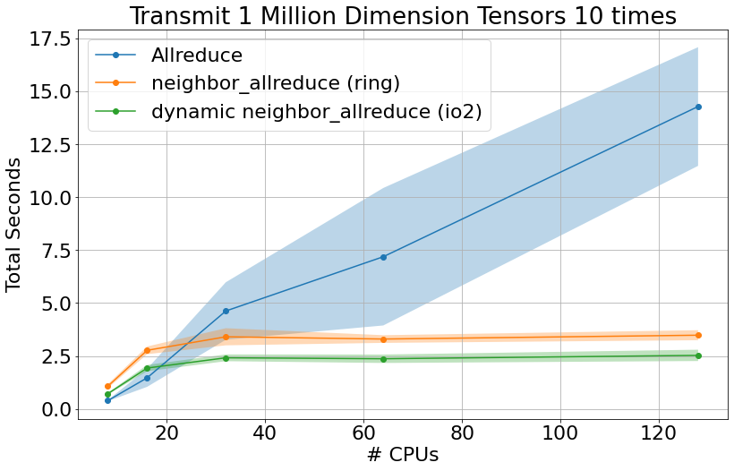
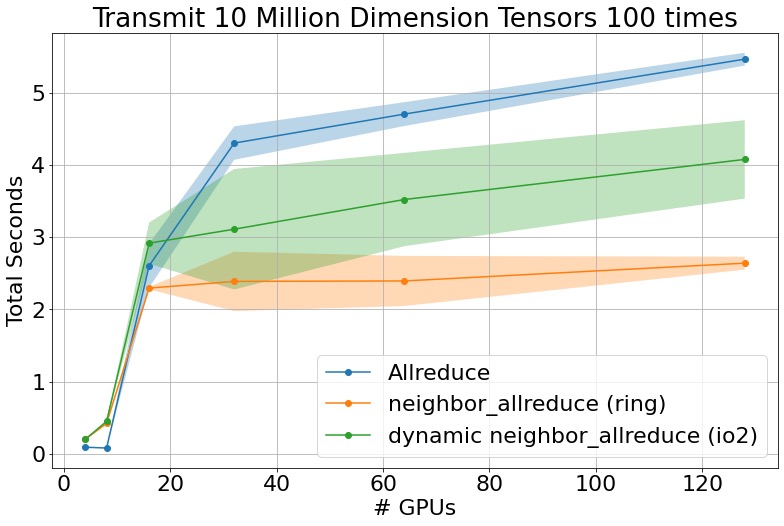
Figure 11: The execution time of allreduce, neighbor allreduce, and dynamic neighbor allreduce based on CPUs (left) and GPUs (right). We perform the execution 10 times to calculate the average execution time represented by the solid points while the shaded areas represent 90% confidence interval.

To fairly compare different neighbor allreduce methods, we select neighbor allreduce on the ring topology and dynamic neighbor allreduce on the inner-outer exponential-2 graph, supported by BlueFog, so that the data size for transfer in each iteration matches. As we can see from Fig. 11, the proposed neighbor allreduce primitives in BlueFog takes much less time for communication than allreduce on both CPUs and GPUs, especially with more computation cores. In addition, the time consumption for neighbor allreduce increases much slowly compared to allreduce as the number of cores increases, indicating better scalability of the neighbor communication methods.

Note that the communication speed on GPU significantly drops from 8 GPUs to 16 GPUs for all the three methods. Remember that a single p3.16xlarge instance only contains 8 GPUs. We conjecture that the high-speed NVLink significantly boosts the communication efficiency within the local machine, while the communication across multiple machines becomes the bottleneck here, which is also supported in the later decentralized DNN benchmarks in Section VII-B as well.

VII-B Decentralized DNN training with BlueFog

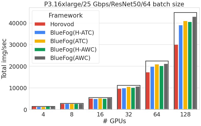
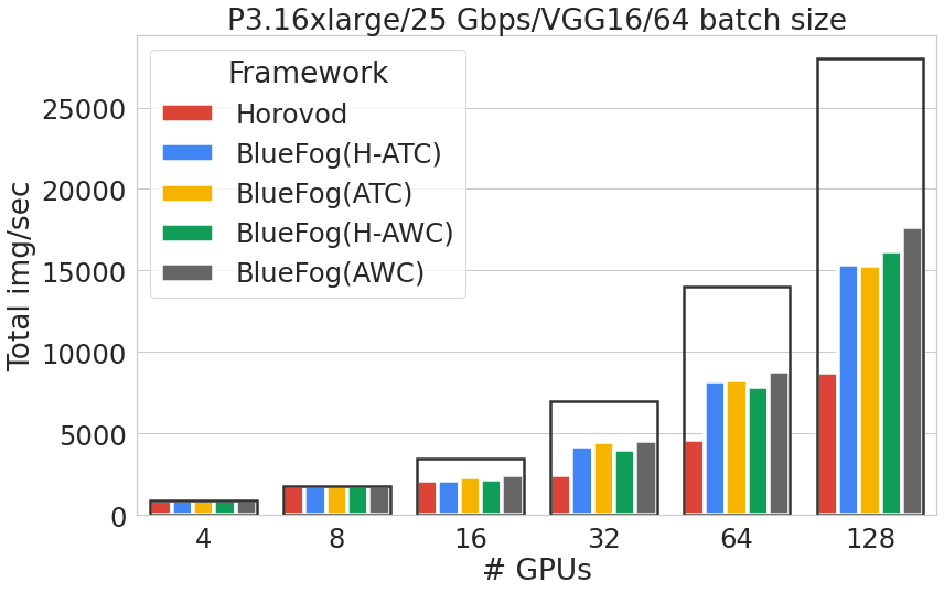
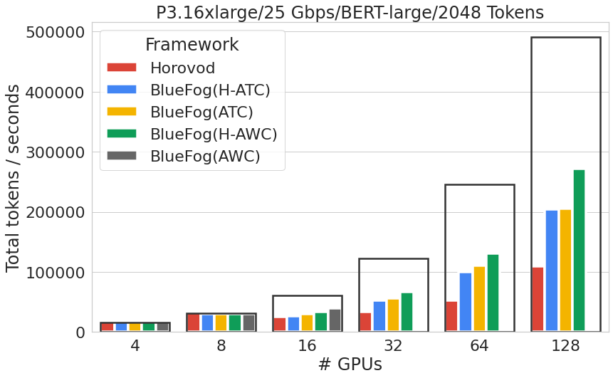
Figure 12: Throughput performance comparison over ResNet-50, VGG-16, and BERT-large models. Label H-ATC represents the hierarchical neighbor allreduce with ATC-style over dynamic exponential 2 topologies. H-AWC is the corresponding AWC-style one. ATC and AWC represents the neighbor allreduce over dynamic inner and outer exponenetial 2 topology with ATC- and AWC- style algorithms. The batch-size or tokens are for one GPU. One machine has 8 GPUs. Hence, for 4 and 8 GPUs data-point, which corresponding to one machine, we use neighbor-allreduce result for hierarchical neighbor-allreduce’s one.

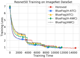
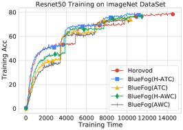
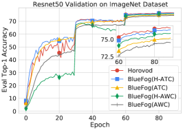
Figure 13: ImageNet training loss and accuracy in terms of wall clock time with ResNet50 and top-1 validation accuracy in terms of epochs.

We demonstrate BlueFog’s performance on decentralized DNN training at different scales. All experiments are done on AWS p3.16xlarge instances. Each instance has 8 Tesla V100 16GB GPUs connected through NVLink. Each pair of instances is connected through a network bandwidth of 25Gbps.

Throughput Benchmark. To begin with, we test the throughput performance over three popular DNN models – ResNet-50[85], VGG-16[86], and BERT-large[87]. First two are both very classical models for image classification and BERT-large is one of the most popular models for natural language processing. The results are shown in Fig. 12. We use Horovod+NCCL as the baseline and run 4 BlueFog supported algorithms, of which are the AWC-style and ATC-style algorithms using neighbor_allreduce and hierarhical_neighbor_allreduce APIs with a dynamic exponential-2 topology respectively [33]. For shortage, we will call them BlueFog(AWC), BlueFog(ATC), BlueFog(H-AWC), and BlueFog(H-ATC).

In term of throughput, the results are quite consistent. No matter which algorithm BlueFog uses, it is always faster than allreduce-style framework, especially when the network size becomes larger. When training with 128 GPUs, the speedup of BlueFog over all-reduce is 1.2x to 1.8x. This is not surprising since the theoretical communication cost and the results in micro-benchmark have already shown that the neighborhood communication is much cheaper than the global allreduce communication. From 4 GPUs to 128 GPUs, the speedup becomes larger. It is reasonable to expect that the advantage of using BlueFog will be even larger with more GPUs.

We do observe that the benchmark we report is relative low in terms of linear scaling up. In the ResNet-50 experiment, BlueFog can reach over 95% scaling efficiency on 128 GPUs, while in VGG and BERT-large experiment, it only reachs around 50-60% efficiency. It is mainly because the experiment environment is 25Gbps without RDMA, which can become the bottleneck of linear scaling up especially for the computation intensive model like BERT-large. In Fig. 12, we can observe the scaling efficiency dramatically dropped from 8 to 16 GPUs, which corresponds to increasing one AWS p3.16xlarge instance to two instances. Within a single instance, the communication between processes is through the high-speed NVLink, which is way faster than inter-machine network. Moreover, note that RestNet-50 has around 23 million parameters, VGG-16 has 138 million parameters, and BERT-large has 345 million parameters. The scaling efficiency are also affected by the number of model parameters, relatively.

Learning Curves. As Bluefog utilizes inexact averaging over different typologies, we further run a series of image classification experiments on ImageNet-1k[8] dataset to validate the performance and generalisation of our system. We train ResNet-50 model following the training protocol of [88]. The Nesterov momentum SGD optimizer is used with a linear scaling learning rate strategy. The left and middle sub-figures in Fig. 13 show the evolution of training loss and accuracy in terms of wall clock time. Compared to Horovod, our implementation of decentralized communication gains 1.3x - 1.43x speed-up with similar convergence. The rightmost sub-figure in Fig. 13 shows the top-1 validation accuracy of the aforementioned decentralized training methods. More convergence results of decentralized optimization algorithms applied on DNN training tasks have also been reported in [3, 2, 68], which should give similar results if implemented in BlueFog.

TABLE II: Comparison training time on 90 epochs ResNet-50 ImageNet and it corresponding validation accuracy between multiple algorithms.

Algorithms	Time(Sec.)	Val. Accuracy	Speed Up
Horovod	14648.26	76.6%	1.00x
BlueFog(H-ATC)	11255.90	76.4%	1.30x
BlueFog(ATC)	10437.62	75.2%	1.40x
BlueFog(H-AWC)	11568.88	75.9%	1.26x
BlueFog(AWC)	10228.92	74.5%	1.43x

More models and algorithms. We further examine the BlueFog over multiple models – ResNet [85], MobileNetv2 [89], and EfficientNet [90], and multiple decentralized algorithms – the vanilla DmSGD [3], DmSGD [61], and QG-DmSGD [67]. The task is the same as the ImageNet classification described before. Table III lists the top-1 validation accuracy comparison across all the models and algorithms. We also list the performance of the parallel SGD using global averaging as the baseline. For each model and algorithm, we examine it over two topology settings, one is the static exponential topology and the other is the dynamic exponential topology. In the latter topology, each process only picks one neighbor at each iteration [33]. The table III shows that the dynamic topology can further reduce the communication cost without any noticeable performance degrade, which is one main reason that BlueFog is designed to support dynamic topologies. The complete freedom of communication control encourages users to develop more efficient decentralized algorithms to train DNNs.

TABLE III: Top-1 validation accuracy and wall-clock time (in hours) comparison with different models and algorithms on ImageNet dataset over static/dynamic exponential topology (8x8 GPUs)[33].

model	ResNet-50		MobileNet-v2		EfficientNet
Topology	static	dynamic	static	dynamic	static	dynamic
Parallel SGD	76.21 (7.0)	-	70.12 (5.8)	-	77.63 (9.0)	-
vanilla DmSGD	76.14 (6.6)	76.06 (5.5)	69.98 (5.6)	69.81 (4.6)	77.62 (8.4)	77.48 (6.9)
DmSGD	76.50 (6.9)	76.52(5.7)	69.62 (5.7)	69.98 (4.8)	77.44 (8.7)	77.51 (7.1)
QG-DmSGD	76.43 (6.6)	76.35(5.6)	69.83 (5.6)	69.81 (4.6)	77.60 (8.4)	77.72 (6.9)

VIII Conclusion

In this paper, we present BlueFog, an open-source library for efficient and high-performance implementation of decentralized algorithms in optimization and deep learning. Through a unified abstraction of different decentralized communication operations, BlueFog provides simple and consistent communication primitives to support diverse decentralized algorithms. BlueFog can be used with PyTorch to train deep neural networks. The system design philosophy and detailed implementation of BlueFog are carefully presented to demonstrate the superior performance. The usage of BlueFog is illustrated with various application examples in optimization and signal processing. Deep learning experiments support that BlueFog outperforms Horovod, a state-of-the-art distributed training framework based on Ring-Allreduce.

IX Acknowledgement

The authors would like to thank Dr. Ji Liu from Baidu Inc. for his contribution to BlueFog and the discussion on the early version of this manuscript, and Edward Nguyen from University California, Los Angeles for contributing to the tutorials on BlueFog.

-A Application example: Exact-Diffusion algorithm

This section still considers the decentralized linear regression problem (15). We will show how to implement Exact-Diffusion [48, 22], a decentralized algorithm that can correct the bias suffered by decentralized gradient descent, over static topology.

Exact-Diffusion. Exact-Diffusion with static graph topology will iterate as follows:

$$\psi_{i}^{(k)} =x_{i}^{(k)}-\gamma A_{i}^{T}(A_{i}x_{i}^{(k)}-b_{i})\hskip 56.9055pt\mbox{(local update)}$$ (24)

$$\phi_{i}^{(k)} =\psi_{i}^{(k)}+x_{i}^{(k)}-\psi_{i}^{(k-1)}\hskip 75.39963pt\mbox{(bias correction)}$$ (25)

$$x_{i}^{(k+1)} =w_{ii}\phi_{i}^{(k)}+\sum_{j\in{\mathcal{N}}(i)}w_{ij}\phi_{j}^{(k)}\hskip 61.17325pt\mbox{(partial averaging)}$$ (26)

where ${\mathcal{N}}(i)$ is the in-coming neighbors of node $i$.

Code. We set the topology as the static ring graph in the following Exact-Diffusion implementation. The code snippet using BlueFog is shown in Listing 6. The complete code can be referred to BlueFog online tutorial.

⬇

1import bluefog.torch as bf

2from bluefog.common import topology_util

3bf.init() # Initialize the BlueFog

4

5# Set topology as static ring graph.

6G = topology_util.RingGraph(bf.size())

7bf.set_topology(G)

8

9# ED implementation

10for ite in range(maxite):

11 grad_local = A.t().mm(A.mm(x) - b) # compute local grad

12 psi = x - gamma * grad_local # local update

13 phi = psi + x - pre_psi # bias correction

14 x = bf.neighbor_allreduce(phi) # partial averaging

15 pre_psi = psi.clone()

Listing 6: BlueFog implmentation of the Exact-Diffusion algorithm to solve decentralized linear regression.

-B Application example: Push-sum gradient tracking algorithm

This section considers the decentralized linear regression problem (15). We will show how to implement push-sum gradient tracking [25] in BlueFog, a decentralized algorithm based on the push-style communication, over time-varying topologies.

Push-sum gradient tracking. The push-sum gradient tracking over time-varying topology will iterate as follows:

$$u_{i}^{(k+1)} =w^{(k)}_{ii}(u_{i}^{(k)}-\gamma y_{i}^{(k)})+\sum_{j\in{\mathcal{N}}(i)}w^{(k)}_{ij}(u_{j}^{(k)}-\gamma y_{j}^{(k)})$$ (27)

$$v_{i}^{(k+1)} =w^{(k)}_{ii}v_{i}^{(k)}+\sum_{j\in{\mathcal{N}}(i)}w^{(k)}_{ij}v_{j}^{(k)}$$ (28)

$$x_{i}^{(k+1)} =u_{i}^{(k+1)}/v_{i}^{(k+1)}$$ (29)

$$g_{i}^{(k+1)} =A_{i}^{T}(A_{i}x_{i}^{(k+1)}-b_{i})$$ (30)

$$y_{i}^{(k+1)} =w^{(k)}_{ii}(y_{i}^{(k)}+g_{i}^{(k+1)}-g_{i}^{(k)})+\sum_{j\in{\mathcal{N}}(i)}w^{(k)}_{ij}\big{(}y_{j}^{(k)}+g_{j}^{(k+1)}-g_{j}^{(k)}\big{)}$$ (31)

where ${\mathcal{N}}(i)$ is the in-coming neighbors of node $i$, and $y_{i}^{(0)}=g_{i}^{(0)}$

Code. We set the topology as the one-peer variant of grid topology. The code snippet using BlueFog is shown in Listing 7. The complete code can be referred to BlueFog online tutorial.

⬇

1import bluefog.torch as bf

2from bluefog.common import topology_util

3bf.init() # Initialize the BlueFog

4

5def Gradient_tracking_one_step(

6 x, y, u, v, prev_grad_local, dynamic_neighbor_gen, x_opt, A, b, gamma=1e-2):

7

8 # Get the update weights

9 dst_neighbors, src_neighbors = next(dynamic_neighbor_gen)

10 src_weights = {r: 1 for r in src_neighbors}

11 self_weight = 1 / (len(dst_neighbors) + 1)

12 dst_weights = {r: self_weight for r in dst_neighbors}

13

14 # u update step: u_{k+1} = W^k (u_k - \alpha*y_k)

15 w = u - alpha * y

16 u_new = bf.neighbor_allreduce(w, self_weight, src_weights, dst_weights)

17

18 # v update: v_{k+1} = W^k v_{k} --- (Correction weights)

19 v_new = bf.neighbor_allreduce(v, self_weight, src_weights, dst_weights)

20

21 # x update: x_{k+1} = u_{k+1} / v_{k+1} (element-wise division)

22 x_new = u_new / v_new

23

24 # y update step: y_{k+1} = W^k (y_k + \grad f(x_{k+1}) - \grad f(x_{k}))

25 grad_local = A.t().mm(A.mm(x_new) - b)

26 q = y + grad_local - prev_grad_local

27 y_new = bf.neighbor_allreduce(q, self_weight, src_weights, dst_weights)

28

29 return x_new, y_new, u_new, v_new, grad_local

30

31# Set up grid topology

32bf.set_topology(topology_util.MeshGrid2DGraph(bf.size()))

33# Set up one-peer variant of the grid topology

34dynamic_neighbor_gen = topology_util.GetDynamicOnePeerSendRecvRanks(bf.load_topology(), bf.rank())

35

36# Algorithm starts

37for ite in range(maxite):

38 x, y, u, v, prev_grad_local = Gradient_tracking_one_step(

39 x, y, u, v, prev_grad_local, dynamic_neighbor_gen, x_opt, A, b, gamma=2e-2)

Listing 7: BlueFog implmentation of the push-sum Gradient-Tracking algorithm over time-varying topologies.

References

- [1] Xiangru Lian, Ce Zhang, Huan Zhang, Cho-Jui Hsieh, Wei Zhang, and Ji Liu, “Can decentralized algorithms outperform centralized algorithms? a case study for decentralized parallel stochastic gradient descent,” in Advances in Neural Information Processing Systems, 2017, pp. 5330–5340.
- [2] Xiangru Lian, Wei Zhang, Ce Zhang, and Ji Liu, “Asynchronous decentralized parallel stochastic gradient descent,” in International Conference on Machine Learning. PMLR, 2018, pp. 3043–3052.
- [3] Mahmoud Assran, Nicolas Loizou, Nicolas Ballas, and Mike Rabbat, “Stochastic gradient push for distributed deep learning,” in International Conference on Machine Learning. PMLR, 2019, pp. 344–353.
- [4] Yiming Chen, Kun Yuan, Yingya Zhang, Pan Pan, Yinghui Xu, and Wotao Yin, “Accelerating gossip SGD with periodic global averaging,” in International Conference on Machine Learning, 2021.
- [5] Kun Yuan, Yiming Chen, Xinmeng Huang, Yingya Zhang, Pan Pan, Yinghui Xu, and Wotao Yin, “DecentLaM: Decentralized momentum SGD for large-batch deep training,” in International Conference on Computer Vision, 2021.
- [6] Jacob Devlin, Ming-Wei Chang, Kenton Lee, and Kristina Toutanova, “Bert: Pre-training of deep bidirectional transformers for language understanding,” in NAACL-HLT (1), 2019.
- [7] Tom Brown, Benjamin Mann, Nick Ryder, Melanie Subbiah, Jared D Kaplan, Prafulla Dhariwal, Arvind Neelakantan, Pranav Shyam, Girish Sastry, Amanda Askell, Sandhini Agarwal, Ariel Herbert-Voss, Gretchen Krueger, Tom Henighan, Rewon Child, Aditya Ramesh, Daniel Ziegler, Jeffrey Wu, Clemens Winter, Chris Hesse, Mark Chen, Eric Sigler, Mateusz Litwin, Scott Gray, Benjamin Chess, Jack Clark, Christopher Berner, Sam McCandlish, Alec Radford, Ilya Sutskever, and Dario Amodei, “Language models are few-shot learners,” in Advances in Neural Information Processing Systems, H. Larochelle, M. Ranzato, R. Hadsell, M. F. Balcan, and H. Lin, Eds. 2020, vol. 33, pp. 1877–1901, Curran Associates, Inc.
- [8] Jia Deng, Wei Dong, Richard Socher, Li-Jia Li, Kai Li, and Li Fei-Fei, “Imagenet: A large-scale hierarchical image database,” in 2009 IEEE conference on computer vision and pattern recognition. Ieee, 2009, pp. 248–255.
- [9] Shibamouli Lahiri, “Complexity of Word Collocation Networks: A Preliminary Structural Analysis,” in Proceedings of the Student Research Workshop at the 14th Conference of the European Chapter of the Association for Computational Linguistics, Gothenburg, Sweden, April 2014, pp. 96–105, Association for Computational Linguistics.
- [10] T Nathan Mundhenk, Goran Konjevod, Wesam A Sakla, and Kofi Boakye, “A large contextual dataset for classification, detection and counting of cars with deep learning,” in European Conference on Computer Vision. Springer, 2016, pp. 785–800.
- [11] Alexander Smola and Shravan Narayanamurthy, “An architecture for parallel topic models,” Proceedings of the VLDB Endowment, vol. 3, no. 1-2, pp. 703–710, 2010.
- [12] Andrew Gibiansky, “Bringing hpc techniques to deep learning,” https://andrew.gibiansky.com/blog/machine-learning/baidu-allreduce/, 2017, Accessed: 2020-08-12.
- [13] Daron Acemoglu, Munther A Dahleh, Ilan Lobel, and Asuman Ozdaglar, “Bayesian learning in social networks,” The Review of Economic Studies, vol. 78, no. 4, pp. 1201–1236, 2011.
- [14] Jon Kleinberg, “Complex networks and decentralized search algorithms,” in Proceedings of the International Congress of Mathematicians (ICM), 2006, vol. 3, pp. 1019–1044.
- [15] Gokhan Inalhan, Dusan M Stipanovic, and Claire J Tomlin, “Decentralized optimization, with application to multiple aircraft coordination,” in Proceedings of the 41st IEEE Conference on Decision and Control, 2002. IEEE, 2002, vol. 1, pp. 1147–1155.
- [16] Shuai Lu, Nader Samaan, Ruisheng Diao, Marcelo Elizondo, Chunlian Jin, Ebony Mayhorn, Yu Zhang, and Harold Kirkham, “Centralized and decentralized control for demand response,” in ISGT 2011. Ieee, 2011, pp. 1–8.
- [17] Edgar Gabriel, Graham E. Fagg, George Bosilca, Thara Angskun, Jack J. Dongarra, Jeffrey M. Squyres, Vishal Sahay, Prabhanjan Kambadur, Brian Barrett, Andrew Lumsdaine, Ralph H. Castain, David J. Daniel, Richard L. Graham, and Timothy S. Woodall, “Open MPI: Goals, concept, and design of a next generation MPI implementation,” in Proceedings, 11th European PVM/MPI Users’ Group Meeting, Budapest, Hungary, September 2004, pp. 97–104.
- [18] “NVIDIA NCCL Document,” https://docs.nvidia.com/deeplearning/nccl/release-notes/rel_2-7-3.html#rel_2-7-3.
- [19] Angelia Nedic and Asuman Ozdaglar, “Distributed subgradient methods for multi-agent optimization,” IEEE Transactions on Automatic Control, vol. 54, no. 1, pp. 48–61, 2009.
- [20] Jianshu Chen and Ali H Sayed, “Diffusion adaptation strategies for distributed optimization and learning over networks,” IEEE Transactions on Signal Processing, vol. 60, no. 8, pp. 4289–4305, 2012.
- [21] Kun Yuan, Bicheng Ying, Xiaochuan Zhao, and Ali H Sayed, “Exact diffusion for distributed optimization and learning—part i: Algorithm development,” IEEE Transactions on Signal Processing, vol. 67, no. 3, pp. 708–723, 2018.
- [22] Zhi Li, Wei Shi, and Ming Yan, “A decentralized proximal-gradient method with network independent step-sizes and separated convergence rates,” IEEE Transactions on Signal Processing, vol. 67, no. 17, pp. 4494–4506, 2019.
- [23] J. Xu, S. Zhu, Y. C. Soh, and L. Xie, “Augmented distributed gradient methods for multi-agent optimization under uncoordinated constant stepsizes,” in IEEE Conference on Decision and Control (CDC), Osaka, Japan, 2015, pp. 2055–2060.
- [24] P. Di Lorenzo and G. Scutari, “Next: In-network nonconvex optimization,” IEEE Transactions on Signal and Information Processing over Networks, vol. 2, no. 2, pp. 120–136, 2016.
- [25] Angelia Nedic, Alex Olshevsky, and Wei Shi, “Achieving geometric convergence for distributed optimization over time-varying graphs,” SIAM Journal on Optimization, vol. 27, no. 4, pp. 2597–2633, 2017.
- [26] G. Qu and N. Li, “Harnessing smoothness to accelerate distributed optimization,” IEEE Transactions on Control of Network Systems, vol. 5, no. 3, pp. 1245–1260, 2018.
- [27] Songtao Lu and Chai Wah Wu, “Decentralized stochastic non-convex optimization over weakly connected time-varying digraphs,” in ICASSP 2020-2020 IEEE International Conference on Acoustics, Speech and Signal Processing (ICASSP). IEEE, 2020, pp. 5770–5774.
- [28] Alexander Sergeev and Mike Del Balso, “Horovod: fast and easy distributed deep learning in TensorFlow,” arXiv preprint arXiv:1802.05799, 2018.
- [29] Anastasia Koloskova, Nicolas Loizou, Sadra Boreiri, Martin Jaggi, and Sebastian U Stich, “A unified theory of decentralized sgd with changing topology and local updates,” in International Conference on Machine Learning (ICML), 2020, pp. 1–12.
- [30] Lingjing Kong, Tao Lin, Anastasia Koloskova, Martin Jaggi, and Sebastian U Stich, “Consensus control for decentralized deep learning,” arXiv preprint arXiv:2102.04828, 2021.
- [31] Sulaiman A Alghunaim and Kun Yuan, “A unified and refined convergence analysis for non-convex decentralized learning,” arXiv preprint arXiv:2110.09993, 2021.
- [32] Ernest K. Ryu and Wotao Yin, Large-Scale Convex Optimization via Monotone Operators, https://large-scale-book.mathopt.com/, 2021.
- [33] Bicheng Ying, Kun Yuan, Yiming Chen, Hanbin Hu, Pan Pan, and Wotao Yin, “Exponential graph is provably efficient for decentralized deep training,” To appear on the 35th conference on Advances in Neural Information Processing Systems. Also available at arXiv:2110.13363, 2021.
- [34] Cassio G Lopes and Ali H Sayed, “Diffusion least-mean squares over adaptive networks: Formulation and performance analysis,” IEEE Transactions on Signal Processing, vol. 56, no. 7, pp. 3122–3136, 2008.
- [35] Tal Ben-Nun and Torsten Hoefler, “Demystifying parallel and distributed deep learning: An in-depth concurrency analysis,” ACM Computing Surveys (CSUR), vol. 52, no. 4, pp. 1–43, 2019.
- [36] Yimin Jiang, Yibo Zhu, Chang Lan, Bairen Yi, Yong Cui, and Chuanxiong Guo, “A unified architecture for accelerating distributed {DNN} training in heterogeneous gpu/cpu clusters,” in 14th {USENIX} Symposium on Operating Systems Design and Implementation ({OSDI} 20), 2020, pp. 463–479.
- [37] Kun Huang and Shi Pu, “Improving the transient times for distributed stochastic gradient methods,” arXiv preprint arXiv:2105.04851, 2021.
- [38] Kun Yuan and Sulaiman A Alghunaim, “Removing data heterogeneity influence enhances network topology dependence of decentralized sgd,” arXiv preprint arXiv:2105.08023, 2021.
- [39] Thijs Vogels, Lie He, Anastasia Koloskova, Tao Lin, Sai Praneeth Karimireddy, Sebastian U Stich, and Martin Jaggi, “Relaysum for decentralized deep learning on heterogeneous data,” To appear on the 35th conference on Advances in Neural Information Processing Systems. Also avaialbe at arXiv:2110.04175, 2021.
- [40] Yucheng Lu and Christopher De Sa, “Optimal complexity in decentralized training,” in International Conference on Machine Learning. PMLR, 2021, pp. 7111–7123.
- [41] Ran Xin, Subhro Das, Usman A Khan, and Soummya Kar, “A stochastic proximal gradient framework for decentralized non-convex composite optimization: Topology-independent sample complexity and communication efficiency,” arXiv preprint arXiv:2110.01594, 2021.
- [42] John Tsitsiklis, Dimitri Bertsekas, and Michael Athans, “Distributed asynchronous deterministic and stochastic gradient optimization algorithms,” IEEE transactions on automatic control, vol. 31, no. 9, pp. 803–812, 1986.
- [43] Ali H Sayed, “Adaptation, learning, and optimization over networks,” Foundations and Trends in Machine Learning, vol. 7, no. ARTICLE, pp. 311–801, 2014.
- [44] John C Duchi, Alekh Agarwal, and Martin J Wainwright, “Dual averaging for distributed optimization: Convergence analysis and network scaling,” IEEE Transactions on Automatic control, vol. 57, no. 3, pp. 592–606, 2011.
- [45] Gonzalo Mateos, Juan Andrés Bazerque, and Georgios B Giannakis, “Distributed sparse linear regression,” IEEE Transactions on Signal Processing, vol. 58, no. 10, pp. 5262–5276, 2010.
- [46] Wei Shi, Qing Ling, Kun Yuan, Gang Wu, and Wotao Yin, “On the linear convergence of the admm in decentralized consensus optimization,” IEEE Transactions on Signal Processing, vol. 62, no. 7, pp. 1750–1761, 2014.
- [47] Wei Shi, Qing Ling, Gang Wu, and Wotao Yin, “Extra: An exact first-order algorithm for decentralized consensus optimization,” SIAM Journal on Optimization, vol. 25, no. 2, pp. 944–966, 2015.
- [48] K. Yuan, B. Ying, X. Zhao, and A. H. Sayed, “Exact dffusion for distributed optimization and learning – Part I: Algorithm development,” IEEE Transactions on Signal Processing, vol. 67, no. 3, pp. 708 – 723, 2019.
- [49] Z. Li, W. Shi, and M. Yan, “A decentralized proximal-gradient method with network independent step-sizes and separated convergence rates,” IEEE Transactions on Signal Processing, July 2019, early acces. Also available on arXiv:1704.07807.
- [50] Kevin Scaman, Francis Bach, Sébastien Bubeck, Yin Tat Lee, and Laurent Massoulié, “Optimal algorithms for smooth and strongly convex distributed optimization in networks,” in International Conference on Machine Learning, 2017, pp. 3027–3036.
- [51] César A Uribe, Soomin Lee, Alexander Gasnikov, and Angelia Nedić, “A dual approach for optimal algorithms in distributed optimization over networks,” Optimization Methods and Software, pp. 1–40, 2020.
- [52] Hanlin Tang, Xiangru Lian, Ming Yan, Ce Zhang, and Ji Liu, “: Decentralized training over decentralized data,” in International Conference on Machine Learning, 2018, pp. 4848–4856.
- [53] Ran Xin, Usman A Khan, and Soummya Kar, “An improved convergence analysis for decentralized online stochastic non-convex optimization,” arXiv preprint:2008.04195, 2020.
- [54] Songtao Lu, Xinwei Zhang, Haoran Sun, and Mingyi Hong, “Gnsd: A gradient-tracking based nonconvex stochastic algorithm for decentralized optimization,” in 2019 IEEE Data Science Workshop (DSW). IEEE, 2019, pp. 315–321.
- [55] Dan Alistarh, Demjan Grubic, Jerry Li, Ryota Tomioka, and Milan Vojnovic, “Qsgd: Communication-efficient sgd via gradient quantization and encoding,” in Advances in Neural Information Processing Systems, 2017, pp. 1709–1720.
- [56] Jeremy Bernstein, Jiawei Zhao, Kamyar Azizzadenesheli, and Anima Anandkumar, “signsgd with majority vote is communication efficient and fault tolerant,” arXiv preprint:1810.05291, 2018.
- [57] Anastasia Koloskova, Tao Lin, Sebastian U Stich, and Martin Jaggi, “Decentralized deep learning with arbitrary communication compression,” in International Conference on Learning Representations, 2019.
- [58] Anastasia Koloskova, Sebastian Stich, and Martin Jaggi, “Decentralized stochastic optimization and gossip algorithms with compressed communication,” in International Conference on Machine Learning, 2019, pp. 3478–3487.
- [59] Hanlin Tang, Chen Yu, Xiangru Lian, Tong Zhang, and Ji Liu, “Doublesqueeze: Parallel stochastic gradient descent with double-pass error-compensated compression,” in International Conference on Machine Learning. PMLR, 2019, pp. 6155–6165.
- [60] Sebastian Urban Stich, “Local sgd converges fast and communicates little,” in International Conference on Learning Representations (ICLR), 2019.
- [61] Hao Yu, Rong Jin, and Sen Yang, “On the linear speedup analysis of communication efficient momentum sgd for distributed non-convex optimization,” in International Conference on Machine Learning. PMLR, 2019, pp. 7184–7193.
- [62] Tianyi Chen, Georgios Giannakis, Tao Sun, and Wotao Yin, “LAG: Lazily aggregated gradient for communication-efficient distributed learning,” in Advances in Neural Information Processing Systems, 2018, pp. 5050–5060.
- [63] Yaohua Liu, Wei Xu, Gang Wu, Zhi Tian, and Qing Ling, “Communication-censored admm for decentralized consensus optimization,” IEEE Transactions on Signal Processing, vol. 67, no. 10, pp. 2565–2579, 2019.
- [64] Martin Abadi, Paul Barham, Jianmin Chen, Zhifeng Chen, Andy Davis, Jeffrey Dean, Matthieu Devin, Sanjay Ghemawat, Geoffrey Irving, Michael Isard, et al., “Tensorflow: A system for large-scale machine learning,” in 12th {USENIX} symposium on operating systems design and implementation ({OSDI} 16), 2016, pp. 265–283.
- [65] Pitch Patarasuk and Xin Yuan, “Bandwidth optimal all-reduce algorithms for clusters of workstations,” Journal of Parallel and Distributed Computing, vol. 69, no. 2, pp. 117–124, 2009.
- [66] Mu Li, David G Andersen, Jun Woo Park, Alexander J Smola, Amr Ahmed, Vanja Josifovski, James Long, Eugene J Shekita, and Bor-Yiing Su, “Scaling distributed machine learning with the parameter server,” in 11th {USENIX} Symposium on Operating Systems Design and Implementation ({OSDI} 14), 2014, pp. 583–598.
- [67] Tao Lin, Sai Praneeth Karimireddy, Sebastian U Stich, and Martin Jaggi, “Quasi-global momentum: Accelerating decentralized deep learning on heterogeneous data,” in International Conference on Machine Learning, 2021.
- [68] Qinyi Luo, Jiaao He, Youwei Zhuo, and Xuehai Qian, “Prague: High-performance heterogeneity-aware asynchronous decentralized training,” in Proceedings of the Twenty-Fifth International Conference on Architectural Support for Programming Languages and Operating Systems, 2020, pp. 401–416.
- [69] Shaoduo Gan, Xiangru Lian, Rui Wang, Jianbin Chang, Chengjun Liu, Hongmei Shi, Shengzhuo Zhang, Xianghong Li, Tengxu Sun, Jiawei Jiang, et al., “Bagua: Scaling up distributed learning with system relaxations,” arXiv preprint arXiv:2107.01499, 2021.
- [70] Shi Pu, Wei Shi, Jinming Xu, and Angelia Nedić, “Push–pull gradient methods for distributed optimization in networks,” IEEE Transactions on Automatic Control, vol. 66, no. 1, pp. 1–16, 2020.
- [71] Ran Xin and Usman A Khan, “A linear algorithm for optimization over directed graphs with geometric convergence,” IEEE Control Systems Letters, vol. 2, no. 3, pp. 315–320, 2018.
- [72] Anthony Williams, C++ concurrency in action, London, 2012.
- [73] Message Passing Interface Forum, “MPI: A Message-Passing Interface Standard Version 3.0,” 09 2012, Chapter author for Collective Communication, Process Topologies, and One Sided Communications.
- [74] William Gropp, Torsten Hoefler, Rajeev Thakur, and Ewing Lusk, Using advanced MPI: Modern features of the message-passing interface, MIT Press, 2014.
- [75] Sheng-Yuan Tu and Ali H Sayed, “Cooperative prey herding based on diffusion adaptation,” in 2011 IEEE International Conference on Acoustics, Speech and Signal Processing (ICASSP). IEEE, 2011, pp. 3752–3755.
- [76] Angelia Nedić and Alex Olshevsky, “Distributed optimization over time-varying directed graphs,” IEEE Transactions on Automatic Control, vol. 60, no. 3, pp. 601–615, 2014.
- [77] Florence Bénézit, Vincent Blondel, Patrick Thiran, John Tsitsiklis, and Martin Vetterli, “Weighted gossip: Distributed averaging using non-doubly stochastic matrices,” in 2010 ieee international symposium on information theory. IEEE, 2010, pp. 1753–1757.
- [78] “NVIDIA DGX-1,” https://www.nvidia.com/en-us/data-center/dgx-1/.
- [79] Paul J Werbos, “Backpropagation through time: what it does and how to do it,” Proceedings of the IEEE, vol. 78, no. 10, pp. 1550–1560, 1990.
- [80] David E Rumelhart, Geoffrey E Hinton, and Ronald J Williams, “Learning internal representations by error propagation,” Tech. Rep., California Univ San Diego La Jolla Inst for Cognitive Science, 1985.
- [81] Adam Paszke, Sam Gross, Francisco Massa, Adam Lerer, James Bradbury, Gregory Chanan, Trevor Killeen, Zeming Lin, Natalia Gimelshein, Luca Antiga, et al., “Pytorch: An imperative style, high-performance deep learning library,” in Advances in neural information processing systems, 2019, pp. 8026–8037.
- [82] William Gropp, Rajeev Thakur, and Ewing Lusk, Using MPI-2: advanced features of the message passing interface, MIT press, 1999.
- [83] “Amazon Web Services,” https://aws.amazon.com/.
- [84] “Amazon EC2 P3 Instances,” https://aws.amazon.com/ec2/instance-types/p3/.
- [85] Kaiming He, Xiangyu Zhang, Shaoqing Ren, and Jian Sun, “Deep residual learning for image recognition,” in Proceedings of the IEEE conference on computer vision and pattern recognition, 2016, pp. 770–778.
- [86] Karen Simonyan and Andrew Zisserman, “Very deep convolutional networks for large-scale image recognition,” arXiv preprint arXiv:1409.1556, 2014.
- [87] Jacob Devlin, Ming-Wei Chang, Kenton Lee, and Kristina Toutanova, “Bert: Pre-training of deep bidirectional transformers for language understanding,” arXiv preprint arXiv:1810.04805, 2018.
- [88] Priya Goyal, Piotr Dollár, Ross Girshick, Pieter Noordhuis, Lukasz Wesolowski, Aapo Kyrola, Andrew Tulloch, Yangqing Jia, and Kaiming He, “Accurate, large minibatch sgd: Training imagenet in 1 hour,” arXiv preprint arXiv:1706.02677, 2017.
- [89] Mark Sandler, Andrew Howard, Menglong Zhu, Andrey Zhmoginov, and Liang-Chieh Chen, “Mobilenetv2: Inverted residuals and linear bottlenecks,” in Proceedings of the IEEE conference on computer vision and pattern recognition, 2018, pp. 4510–4520.
- [90] Mingxing Tan and Quoc Le, “Efficientnet: Rethinking model scaling for convolutional neural networks,” in International Conference on Machine Learning. PMLR, 2019, pp. 6105–6114.