Scaling description of creep flow in amorphous solids

Abstract

Amorphous solids such as coffee foam, toothpaste or mayonnaise display a transient creep flow when a stress $\Sigma$ is suddenly imposed. The associated strain rate is commonly found to decay in time as $\dot{\gamma}\sim t^{-\nu}$, followed either by arrest or by a sudden fluidisation. Various empirical laws have been suggested for the creep exponent $\nu$ and fluidisation time $\tau_{f}$ in experimental and numerical studies. Here, we postulate that plastic flow is governed by the difference between $\Sigma$ and the transient yield stress $\Sigma_{t}(\gamma)$ that characterises the stability of configurations visited by the system at strain $\gamma$. Assuming the analyticity of $\Sigma_{t}(\gamma)$ allows us to predict $\nu$ and asymptotic behaviours of $\tau_{f}$ in terms of properties of stationary flows. We test successfully our predictions using elastoplastic models and published experimental results.

Amorphous materials including atomic glasses, colloidal suspensions, dense emulsions or foams are important in industry and engineering Andreotti et al. (2013); Bonn et al. (2017). From a fundamental viewpoint, their properties are mesmerizing: (i) Under quasi-static loading they can display an avalanche-type response Maloney and Lemaitre (2006) near their yield stress $\Sigma_{c}$. (ii) For $\Sigma>\Sigma_{c}$, they can present a singular flow curve, corresponding to the so-called Herschel-Bulkley’s law Herschel and Bulkley (1926) where the strain rate follows $\dot{\gamma}\approx c(\Sigma-\Sigma_{c})^{\beta}$ with $c$ a material-specific constant and $\beta>1$, see e.g. Lin et al. (2014). We restrict ourselves to materials with such flow curves. (iii) Depending on the system preparation the transient response to an applied strain can be smooth, or discontinuous if a narrow shear band appears Ozawa et al. (2018); Popović et al. (2018); Fielding (2021). Here we focus on (iv) creep flows, another transient phenomenon observed when a constant stress $\Sigma$ is imposed at time $t=0$ on an initial state at zero applied stress. Transiently, a flow rate $\dot{\gamma}\sim t^{-\nu}$ is observed. At low $\Sigma$, flow eventually arrests. However, at sufficiently high $\Sigma$, $\dot{\gamma}(t)$ can be non-monotonic: a sudden fluidisation may occur at some time $\tau_{f}$. Commonly, the creep flow exponent $\nu$ is measured preceding the fluidisation and reported in the range $0.34-1.2$ in experiments Bauer et al. (2006); Caton and Baravian (2008); Divoux et al. (2011); Siebenbürger et al. (2012); Grenard et al. (2014); Leocmach et al. (2014) and particle simulations Chaudhuri and Horbach (2013); Landrum et al. (2016); Cabriolu et al. (2019). By contrast, the creep flow arrest is much less studied Siebenbürger et al. (2012), and $\tau_{f}$ is often reported using phenomenological fitting functions, including: (a) A power law $\tau_{f}\sim(\Sigma-\Sigma_{0})^{-b}$ (with both $b$ and $\Sigma_{0}$ fitting parameters) in experiments on carbopol microgel Divoux et al. (2011), protein gels Leocmach et al. (2014), and colloidal glasses Siebenbürger et al. (2012); and particle simulations Chaudhuri and Horbach (2013). (b) An exponential $\ln\tau_{f}\sim-\Sigma$ in experiments on carbon black gels Gibaud et al. (2010); Grenard et al. (2014) and silica gels Sprakel et al. (2011).

From a computational viewpoint, studies of creep flow in athermal elastoplastic models Nicolas et al. (2018) report (a) $\tau_{f}\sim(\Sigma-\Sigma_{0})^{-b}$ with a preparation-dependent exponent $b\simeq 1.7-2.2$ in a two-dimensional model Liu et al. (2018a) and $b\simeq 1.3-2.2$ in a mean-field model Liu et al. (2018b). At finite temperature, both models are consistent with (b) $\ln\tau_{f}\sim-\Sigma$ Merabia and Detcheverry (2016). The creep exponent $\nu$ was observed to be unity Bouttes and Vandembroucq (2013) or to be preparation dependent Merabia and Detcheverry (2016). Theoretical approaches supporting particular fitting choices are mostly lacking. A notable exception is the continuum model of shear banding Benzi et al. (2019) that proposes $b=9\beta/4$.

Here, we introduce a theoretical framework that predicts the exponent $\nu$, the asymptotic properties of $\tau_{f}$, and their dependence on temperature. We focus on long time scales and assume that flow is then essentially plastic, thus neglecting the elastic contribution to the strain. We expect this assumption to hold in the materials we consider here, coined “simple yield stress fluids” Ovarlez et al. (2013) such as foams, emulsions or repulsive colloidal glasses. It does not hold in materials with a very slow linear visco-elastic response that can contribute to creep Aime et al. (2018a, b); Leocmach et al. (2014). We also exclude loosely connected colloidal gels, which can display non-monotonic flow curves and sudden transition between distinct structures Lindström et al. (2012); Cho and Bischofberger (2021). Our central hypotheses are that the plastic flow is governed by $\Sigma-\Sigma_{t}(\gamma)$, where $\Sigma_{t}(\gamma)$ is a smooth function of plastic strain $\gamma$ that characterises the stability of configurations visited by the system at a strain $\gamma$. These assumptions lead to a comprehensive description of creep flows in terms of the Herschel-Bulkley exponent $\beta$, as is summarised in Table 1 for athermal and Table 2 for thermal systems. We confirm our predictions in two-dimensional and mean field elastoplastic models. We find that our athermal predictions are also in good agreement with experiments on carbopol microgel and colloidal glasses, while our thermal predictions are consistent with experiments on kaolin suspensions and ketchup.

Theory: The transient response of amorphous materials strongly depends on preparation. For example, the quasistatic stress vs plastic strain curve can increase monotonically or overshoot Andreotti et al. (2013); Antonaglia et al. (2015); Ozawa et al. (2018) as the stability of the system preparation increases. During quasistatic loading the system is at the stress which the material can withhold without flowing at plastic strain $\gamma$. Here, we define the transient yield stress $\Sigma_{t}(\gamma;\Sigma,T)$ that characterizes the stability of the material for non-quasistatic loading. At zero temperature $T$, its definition is:

$$\dot{\gamma}\equiv c\left(\Sigma-\Sigma_{t}(\gamma;\Sigma,T=0)\right)^{\beta}\quad,$$ (1)

To lighten notations, when possible we omit the dependence of $\Sigma_{t}$ on $\Sigma$ and $T$ and simply write it $\Sigma_{t}(\gamma)$. From Eq. (1), it follows that the flow arrests at the finite strain $\gamma_{a}$ for which $\Sigma_{t}(\gamma_{a})=\Sigma$, while in the steady state $\Sigma_{t}(\gamma\to\infty)=\Sigma_{c}$. Note that $\Sigma_{t}(\gamma)$ so defined can be measured by observing the creep flow dynamics and inverting Eq. (1), as performed below. Our central result is that simply assuming that $\Sigma_{t}(\gamma)$ is a smooth is sufficient to determine the creep flow exponent $\nu$ and the fluidisation time $\tau_{f}$, see Fig. 1b. $\Sigma_{t}(\gamma)$ in general depends on the preparation of the system, similar to the quasistatic stress vs strain curve. Here, we focus on the creep flow in systems where $\Sigma_{t}(\gamma)$ overshoots to a maximal value $\Sigma_{M}$ before reaching its steady state value $\Sigma_{c}$, as illustrated in Fig. 1a. The case where $\Sigma_{t}(\gamma)$ does not overshoot, and instead grows monotonically can be treated with the same arguments. As shown in the Supplemental Material (SM), the strain rate monotonically decreases to the steady state value.

At low imposed stresses $\Sigma<\Sigma_{M}$, the flow arrests at a finite $\gamma_{a}$ (see Fig. 1a) where $\Sigma_{t}(\gamma_{a})=\Sigma$. By expanding $\Sigma_{t}\simeq\Sigma_{t}(\gamma_{a})+\partial_{\gamma}\Sigma_{t}(\gamma_{a})(\gamma-\gamma_{a})$ and using Eq. (1), one obtains $\dot{\gamma}\sim(\gamma_{a}-\gamma)^{\beta}$ implying $\dot{\gamma}\sim t^{-\beta/(\beta-1)}$. Instead, for $\Sigma=\Sigma_{M}=\max_{\gamma}\Sigma_{t}(\gamma)=\Sigma_{t}(\gamma_{M})$, a second order expansion implies that $\Sigma_{t}(\gamma)\approx\Sigma_{M}+\partial^{2}_{\gamma}\Sigma_{t}(\gamma_{M})(\gamma-\gamma_{M})^{2}/2$. Using again Eq. (1) one gets $\dot{\gamma}\sim(\gamma_{M}-\gamma)^{2\beta}$ and therefore $\dot{\gamma}\sim t^{-2\beta/(2\beta-1)}$. Finally, for $\Sigma>\Sigma_{M}$ the flow transiently slows down, reaching its minimum at $\gamma_{M}$. In the vicinity of $\gamma_{M}$, one has $\dot{\gamma}\sim[\Sigma-\Sigma_{M}+\partial^{2}_{\gamma}\Sigma_{t}(\gamma_{M})(\gamma_{M}-\gamma)^{2}/2]^{\beta}$. The fluidisation time $\tau_{f}$ is the time at which $\gamma_{M}$ is reached. It is dominated by the time spent approaching $\gamma_{M}$ in an interval of strain of order $\Delta\gamma\sim(\Sigma-\Sigma_{M})^{1/2}$, at a pace $\dot{\gamma}\sim(\Sigma-\Sigma_{M})^{\beta}$, leading to a time $\tau_{f}\sim\Delta\gamma/\dot{\gamma}\sim\left(\Sigma-\Sigma_{M}\right)^{1/2-\beta}$. We summarise the athermal creep flow results in Table 1.

(a)

(b)

(c)

(d)

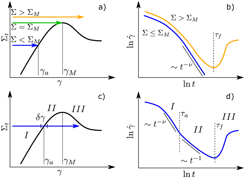
Figure 1: Left: Sketch of $\Sigma_{t}(\gamma;\Sigma,T)$ for (a) $T=0$ and (c) $T>0$. Arrows indicate different applied stresses $\Sigma$ that lead to creep flow scenarios discussed in the text. Right: The corresponding sketch of the creep flow, respectively in (b) and (d). $\gamma_{a}(\Sigma)$ is defined by $\Sigma=\Sigma_{t}(\gamma_{a},\Sigma,T)$ and $\gamma_{M}=\gamma_{a}(\Sigma_{M})$.

${\Sigma<\Sigma_{M}}$	$\nu=\frac{\beta}{\beta-1}$
${\Sigma=\Sigma_{M}}$	$\nu=\frac{2\beta}{2\beta-1}$
${\Sigma>\Sigma_{M}}$	${\tau_{f}\sim(\Sigma-\Sigma_{M})^{\frac{1}{2}-\beta}}$

Table 1: Main results for athermal creep flow, illustrated in Fig. 1a. The corresponding creep flow scenarios are illustrated in Fig. 1b, and corresponding numerical tests are shown in Fig. 2.

For a small finite temperature $T$ , $\Sigma_{t}(\gamma;\Sigma,T)$ can now be defined from the finite temperature stationary flow curves. Our qualitative results are robust to details of the functional form chosen for these curves. Quantitatively, theoretical arguments and elastoplastic models Chattoraj et al. (2010); Purrello et al. (2017); Ferrero et al. (2021); Popović et al. (2021a) support that the steady state flow follows a scaling relation: $\dot{\gamma}=T^{\psi}f((\Sigma-\Sigma_{c})/T^{1/\alpha})$. Here, $\psi=\beta/\alpha$, where the parameter $\alpha$ describes the microscopic potential. The scaling function $f$ must be such that $\dot{\gamma}$ converges to $\dot{\gamma}\sim(\Sigma-\Sigma_{c})^{\beta}$ (the Herschel-Bulkley law) in the limit $T\to 0$, i.e. $f(x)\sim x^{\beta}$ for $x\rightarrow\infty$. For negative arguments, $f$ describes thermal activation so that $f(x)\sim\exp(-C_{0}x^{\alpha})$ for $x\rightarrow-\infty$, where $C_{0}>0$.

We thus define the transient yield stress at finite $T$ as:

$$\dot{\gamma}\equiv T^{\psi}f\left(\frac{\Sigma-\Sigma_{t}(\gamma;\Sigma,T)}{T^{1/\alpha}}\right)\quad.$$ (2)

Here we discuss systems where $\Sigma_{t}(\gamma)$ overshoots, as illustrated in Figs. 1c and 1d, see SM for the monotonic case, which includes Ref. Lin et al. (2015). Initially at small strains thermal fluctuations are negligible and the creep flow exponent follows the athermal prediction $\dot{\gamma}\sim t^{-\beta/(\beta-1)}$. This regime is valid until a plastic strain $\gamma_{a}$ for which $\Sigma\simeq\Sigma_{t}(\gamma_{a})$, where Eq. (2) implies that the flow rate follows $\dot{\gamma}\sim T^{\psi}$. Comparing these two expressions, the crossover time where thermal activation starts to play a role follows $\tau_{a}\sim T^{(1-\beta)/\alpha}$. This cross-over occurs on a strain increment $\delta\gamma$ (see Fig. 1c), which corresponds to the argument of $f$ in Eq. (2) becoming negative and ${\cal O}(1)$. Expanding this argument using $\Sigma-\Sigma_{t}(\gamma)\sim\gamma_{a}-\gamma$ leads to $\delta\gamma\sim T^{1/\alpha}$. Beyond the crossover $\gamma-\gamma_{a}\gg\delta\gamma$, flow is dominated by thermal activation. This corresponds to the exponential behaviour of $f(x)$ for large negative arguments. It is then straightforward (see SM) to obtain from Eq. (2) and the linearization $\Sigma-\Sigma_{t}(\gamma)\sim\gamma_{a}-\gamma$ that the strain grows logarithmically in time, implying that $\dot{\gamma}\sim t^{-1}$ at long times. Finally, for $\gamma>\gamma_{M}$ the flow rate rises and fluidisation occurs. In contrast to athermal systems, fluidisation also occurs for $\Sigma<\Sigma_{M}$. We can estimate the fluidisation time in the limit of small temperatures, as the time spent in the vicinity of $\gamma_{M}$. For $\Sigma<\Sigma_{M}$, expanding $\Sigma_{t}(\gamma)$ around $\gamma_{M}$ in Eq. 2 and using the scaling function form we derived previously Popović et al. (2021a), we find $\tau_{f}\sim(T/(\Sigma_{M}-\Sigma)^{\alpha-1})^{1/2-\beta}\exp[(C_{0}(\Sigma_{M}-\Sigma)^{\alpha}/T)]$. For $\Sigma>\Sigma_{M}$ the flow is predominantly athermal, except for $(\Sigma-\Sigma_{M})^{\alpha}\leq T$ where $\dot{\gamma}\sim T^{\psi}$ for strains near $\gamma_{M}$ on an interval that scales as $\Delta\gamma=\gamma_{M}-\gamma\sim T^{1/(2\alpha)}$, leading to a fluidisation time $\tau_{f}\sim\Delta\gamma/\dot{\gamma}\sim T^{(1/2-\beta)/\alpha}$.

(a)

(b)

(c)

(d)

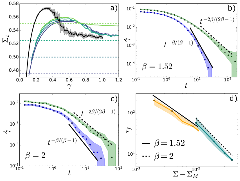
Figure 2: Creep flow in athermal elasto-plastic models: (a) Transient yield stress curves $\Sigma_{t}(\gamma)$ at stresses indicated by the dashed lines, at $T=0.002$. For reference, the quasistatic stress vs plastic strain curve is shown in black. (b, c) Median values of creep flow at two imposed stresses: blue circles ($\Sigma<\Sigma_{M}$), green triangles ($\Sigma=\Sigma_{M}$). Black lines indicate the corresponding predicted power laws, see Table 1. (d) Fluidisation times in $2d$ (yellow circles) and mean field (cyan squares). In all plots shaded regions correspond to $25\text{th}$-$75\text{th}$ percentile range.

athermal to thermal transition width	$\delta\gamma\sim T^{1/\alpha}$
athermal to thermal transition time	${\tau_{a}\sim T^{(\beta-1)/\alpha}}$
thermal creep flow	$\nu=1$
fluidisation time	$\tau_{f}\sim(\frac{T}{(\Sigma_{M}-\Sigma)^{\alpha-1}})^{\frac{1}{2}-\beta}e^{c_{T}\frac{(\Sigma_{M}-\Sigma)^{\alpha}}{T}}$

Table 2: Main results for thermal creep flow. The corresponding numerical tests are shown in Fig. 3.

Numerical simulations: To test the proposed creep exponents we simulate creep flow using a two-dimensional elastoplastic Popović et al. (2021a) (see SM, which includes Ref. Picard et al. (2005)), whereby we benefit for previously measured exponent $\beta=1.52$ Lin et al. (2014) and scaling function $f$ Popović et al. (2021a).

To estimate the athermal transient yield stress function $\Sigma_{t}(\gamma;\Sigma,T=0)$, we measure $\dot{\gamma}(t)$ at a tiny temperature $T=0.002$ and then numerically invert Eq. 2 using the previously measured $f$ Popović et al. (2021a), as shown in Fig. 2a. We use a tiny but finite temperature to probe $\Sigma_{t}$ beyond the strain $\gamma_{a}$ at which athermal creep would arrest. We find that $\Sigma_{t}$ changes with $\Sigma$, but this dependence is weak. More importantly, our observations are consistent with our smoothness assumption. For comparison, we show the quasistatic stress vs plastic strain curve in the same system, which is clearly different from $\Sigma_{t}(\gamma)$.

We simulate the athermal creep flow at stresses $\Sigma\leq\Sigma_{M}$, see Fig. 2b. The measured creep flow dynamics is consistent with predictions summarised in Table 1. To further test our predictions, we use a mean-field version of elastoplastic model Popović et al. (2021b), which corresponds to a version of Hébraud-Lequeux model Hébraud and Lequeux (1998) where $\beta=2$. We again find that creep flow dynamics is consistent with our predictions, see Fig. 2c.

Finally, for imposed stresses $\Sigma>\Sigma_{M}$ we measure the fluidisation times $\tau_{f}$ as a function of the imposed stress $\Sigma$ in both models, as shown in Fig. 2d. Although the range of data is less than a decade, the changes in the asymptotic behaviour of $\tau_{f}$ are consistent with our predictions, for both values of $\beta$.

(a)

(b)

(c)

(d)

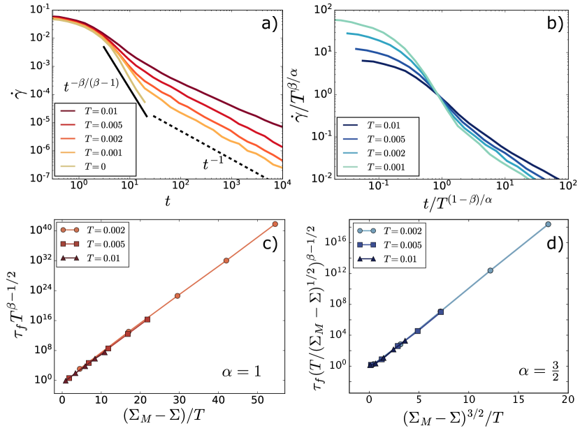
Figure 3: Creep flow in thermal $2d$ elastoplastic model: (a) Athermal and thermal creep regimes follow the predicted flow rate exponents. (b) Rescaling flow rate and time collapses the crossing point of all curves, confirming the existence of a crossover time scale $\tau_{a}\sim T^{(1-\beta)/\alpha}$. (c, d) Fluidisation times $\tau_{f}$ measured with $\alpha=1$ (c) and $\alpha=3/2$ (d) at different temperatures are consistent with our prediction.

We next turn to thermal systems. We first study the transition from the athermal to the thermal creep regime, sketched in Figs. 1c and 1d. In Fig. 3a we show creep curves for $\alpha=3/2$ at $\Sigma=0.45$ in a system with an overshoot in $\Sigma_{t}(\gamma)$. As the temperature is decreased towards $T=0$, the transition between the athermal regime ($\dot{\gamma}\sim t^{-\beta/(\beta-1)}$) and thermal creep ($\dot{\gamma}\sim t^{-1}$) is indeed observed, and occurs at later times following $T^{(1-\beta)/\alpha}$, as confirmed in Fig. 3b.

Finally, we measure fluidisation times of thermal creep flow at different temperatures and imposed stresses both for $\alpha=1$ (Fig. 3c) and $\alpha=3/2$ (Fig. 3d). Following Caton and Baravian (2008), we define the fluidisation time as the time corresponding to the minimum of the flow rate. We find an excellent collapse of the data, confirming our prediction $\tau_{f}\sim(T/(\Sigma_{M}-\Sigma)^{\alpha-1})^{1/2-\beta}\exp[(C_{0}(\Sigma_{M}-\Sigma)^{\alpha}/T)]$.

Note that our theory predicts asymptotic fluidisation and creep exponents in the limit of vanishing flow. Therefore, the effective values extracted from the whole range of measured fluidisation times will in general differ from our measurements. This could account for the differences to the preparation dependent effective exponents reported in the extensive numerical simulations of athermal creep in elastoplastic models Liu et al. (2018a).

Experimental tests: We compare our results the experimental data from carbopol microgel creep experiments Divoux et al. (2011), reproduced in Fig. 4a. At imposed stress values just below the fluidisation stress, the creep exponent is consistent with our prediction $\nu=2\beta/(2\beta-1)$, where we use $1/\beta=0.53$ measured by Divoux et al. (2011). We then extract the fluidisation times from the minima of the flow curves both in this experiment and in the colloidal glass experiment of Siebenbürger et al. (2012). As shown in Fig. 4b, it is consistent with our athermal prediction $\tau_{f}\sim(\Sigma-\Sigma_{M})^{1/2-\beta}$, as indicated by the black line, where the value of $\Sigma_{M}$ is estimated as the highest reported stress value for which no fluidisation is observed, and we use $\beta=1.89$ from Divoux et al. (2011).

Note that another definition of fluidization time $\tau_{f}^{*}$, corresponding to the inflection point of the creep curve, was used in Divoux et al. (2011); Gibaud et al. (2010); Grenard et al. (2014). $\tau_{f}^{*}$ is associated with the emergence of shear banding Divoux et al. (2011); Benzi et al. (2019). Our theory for fluidization, which assumes a homogeneous flow and does not capture shear banding, may thus apply as long $\tau_{f}\leq\tau_{f}^{*}$. This inequality is fulfilled in the cited examples, and also in theoretical treatment supporting that the flow remains homogeneous before $\tau_{f}$ Moorcroft and Fielding (2013).

Concerning thermally activated creep flow, we predict an exponential dependence of $\tau_{f}$ on $\Sigma$, which was indeed reported in carbon black gels Gibaud et al. (2010); Grenard et al. (2014), and in numerical simulations of thermally activated flow in elastoplastic models Merabia and Detcheverry (2016). Likewise, our prediction for the thermal creep flow regime $\dot{\gamma}\sim t^{-1}$ is found in numerical simulations of thermally activated flow Bouttes and Vandembroucq (2013). This behavior is also found in kaolin suspensions Uhlherr et al. (2005) and ketchup Caton and Baravian (2008). However, the validity of our approach to these materials is less clear, as their flow curves need not follow a Herschel-Bulkley law as we assume. They can be instead thixotropic materials with non-monotonic flow curves Ovarlez et al. (2009), known to shear band in stationary flows.

Discussion: We have provided a theoretical framework in which creep flows are controlled by the stress $\Sigma_{t}$ at which configurations visited at time $t$ would stop flowing. Our treatment is similar in spirit to the Landau theory of a phase transition: assuming the analyticity of $\Sigma_{t}$ enables one to express the asymptotic behaviours of creep flows in terms of the better understood stationary flows. Our analysis predicts a rich set of regimes, which is consistent with observations in elastoplastic models and in experiments.

Usual mean-field approaches, both for the yielding transition in amorphous solids Hébraud and Lequeux (1998); Lin and Wyart (2016) and for the depinning transition Fisher (1998), consider the dynamics of the distribution $P(x)$, where $x$ is a local variable indicating how much additional shear stress is required to have a plastic event. In such models, rate of plastic activity following some initial condition was computed at $\Sigma=0$ and $T=0$ Sollich et al. (1997); Parley et al. (2020). These results are consistent with our prediction for $\nu$, supporting that our assumption of analyticity is equivalent to mean-field approaches as is the case in Landau theory.

Our assumption should thus break down when spatial correlations are large, which occurs in particular if avalanches are compact objects. It is the case for short-range depinning phenomena if the spatial dimension satisfies $d<4$, in that case an alternative real space scaling approach summarised in the SM is needed, which includes Refs. Kolton et al. (2006); Ferrero et al. (2013). By contrast, we expect our analysis to hold if $d\geq 4$, or in amorphous solids since in that case avalanches are not compact: the density of plastic events within them vanishes as the avalanche linear extension grows Lin et al. (2014); Nicolas et al. (2018).

(a)

(b)

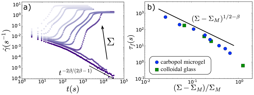
Figure 4: (a) Creep flow of carbopol microgel Divoux et al. (2011) at: $\Sigma[\text{Pa}]=35,36,37,38,40,43,45,50,55,60$ (from bottom to top). The arresting curves are consistent with our prediction (black line). (b) Fluidisation times (see main text for measurement) of carbopol microgel Divoux et al. (2011) (blue circles) and colloidal glass Siebenbürger et al. (2012) (green squares) together with our prediction.

Acknowledgments T.G. acknowledges support from The Netherlands Organisation for Scientific Research (NWO) by a NWO Rubicon Grant 680-50-1520 and from the Swiss National Science Foundation (SNSF) by the SNSF Ambizione Grant No. PZ00P2_185843. The project was supported by the Simons Foundation Grant (No. 454953 Matthieu Wyart) and from the SNSF under Grant No. 200021-165509.

References

- Andreotti et al. (2013) B. Andreotti, Y. Forterre, and O. Pouliquen, Granular media: between fluid and solid (Cambridge University Press, 2013).
- Bonn et al. (2017) D. Bonn, M. M. Denn, L. Berthier, T. Divoux, and S. Manneville, Reviews of Modern Physics 89 (2017), 10.1103/RevModPhys.89.035005.
- Maloney and Lemaitre (2006) C. E. Maloney and A. Lemaitre, Physical Review E 74 (2006), 10.1103/PhysRevE.74.016118.
- Herschel and Bulkley (1926) W. H. Herschel and R. Bulkley, Kolloid-Zeitschrift 39, 291 (1926).
- Lin et al. (2014) J. Lin, E. Lerner, A. Rosso, and M. Wyart, Proceedings of the National Academy of Sciences 111, 14382–14387 (2014).
- Ozawa et al. (2018) M. Ozawa, L. Berthier, G. Biroli, A. Rosso, and G. Tarjus, Proc. Natl. Acad. Sci. 115, 6656 (2018).
- Popović et al. (2018) M. Popović, T. W. J. de Geus, and M. Wyart, Physical Review E 98 (2018), 10.1103/PhysRevE.98.040901.
- Fielding (2021) S. M. Fielding, “Yielding, shear banding and brittle failure of amorphous materials,” (2021), arXiv:2103.06782 [cond-mat.stat-mech] .
- Bauer et al. (2006) T. Bauer, J. Oberdisse, and L. Ramos, Physical Review Letters 97 (2006), 10.1103/PhysRevLett.97.258303.
- Caton and Baravian (2008) F. Caton and C. Baravian, Rheologica Acta 47, 601–607 (2008).
- Divoux et al. (2011) T. Divoux, C. Barentin, and S. Manneville, Soft Matter 7, 8409 (2011).
- Siebenbürger et al. (2012) M. Siebenbürger, M. Ballauff, and T. Voigtmann, Physical Review Letters 108 (2012), 10.1103/PhysRevLett.108.255701.
- Grenard et al. (2014) V. Grenard, T. Divoux, N. Taberlet, and S. Manneville, Soft Matter , 17 (2014).
- Leocmach et al. (2014) M. Leocmach, C. Perge, T. Divoux, and S. Manneville, Physical Review Letters 113 (2014), 10.1103/PhysRevLett.113.038303.
- Chaudhuri and Horbach (2013) P. Chaudhuri and J. Horbach, Physical Review E 88, 040301 (2013).
- Landrum et al. (2016) B. J. Landrum, W. B. Russel, and R. N. Zia, Journal of Rheology 60, 783–807 (2016).
- Cabriolu et al. (2019) R. Cabriolu, J. Horbach, P. Chaudhuri, and K. Martens, Soft Matter 15, 415 (2019).
- Gibaud et al. (2010) T. Gibaud, D. Frelat, and S. Manneville, Soft Matter 6, 3482 (2010).
- Sprakel et al. (2011) J. Sprakel, S. B. Lindström, T. E. Kodger, and D. A. Weitz, Physical Review Letters 106 (2011), 10.1103/PhysRevLett.106.248303.
- Nicolas et al. (2018) A. Nicolas, E. E. Ferrero, K. Martens, and J.-L. Barrat, Reviews of Modern Physics 90 (2018), 10.1103/RevModPhys.90.045006.
- Liu et al. (2018a) C. Liu, E. E. Ferrero, K. Martens, and J.-L. Barrat, Soft Matter 14, 8306 (2018a).
- Liu et al. (2018b) C. Liu, K. Martens, and J.-L. Barrat, Phys. Rev. Lett. 120, 028004 (2018b).
- Merabia and Detcheverry (2016) S. Merabia and F. Detcheverry, EPL (Europhysics Letters) 116, 46003 (2016).
- Bouttes and Vandembroucq (2013) D. Bouttes and D. Vandembroucq, AIP Conference Proceedings 1518, 481 (2013), https://aip.scitation.org/doi/pdf/10.1063/1.4794621 .
- Benzi et al. (2019) R. Benzi, T. Divoux, C. Barentin, S. Manneville, M. Sbragaglia, and F. Toschi, Physical Review Letters 123, 248001 (2019).
- Ovarlez et al. (2013) G. Ovarlez, L. Tocquer, F. Bertrand, and P. Coussot, Soft Matter 9, 5540 (2013).
- Aime et al. (2018a) S. Aime, L. Ramos, and L. Cipelletti, Proceedings of the National Academy of Sciences 115, 3587 (2018a).
- Aime et al. (2018b) S. Aime, L. Cipelletti, and L. Ramos, Journal of Rheology 62, 1429–1441 (2018b).
- Lindström et al. (2012) S. B. Lindström, T. E. Kodger, J. Sprakel, and D. A. Weitz, Soft Matter 8, 3657 (2012).
- Cho and Bischofberger (2021) J. H. Cho and I. Bischofberger, arXiv preprint arXiv:2112.04546 (2021).
- Antonaglia et al. (2015) J. Antonaglia, X. Xie, G. Schwarz, M. Wraith, J. Qiao, Y. Zhang, P. Liaw, J. Uhl, and K. Dahmen, Sci. Rep. 4, 4382 (2015).
- Chattoraj et al. (2010) J. Chattoraj, C. Caroli, and A. Lemaitre, Physical Review Letters 105, 266001 (2010).
- Purrello et al. (2017) V. H. Purrello, J. L. Iguain, A. B. Kolton, and E. A. Jagla, Physical Review E 96 (2017), 10.1103/PhysRevE.96.022112.
- Ferrero et al. (2021) E. E. Ferrero, A. B. Kolton, and E. A. Jagla, Phys. Rev. Materials 5, 115602 (2021).
- Popović et al. (2021a) M. Popović, T. W. J. de Geus, W. Ji, and M. Wyart, Physical Review E 104, 025010 (2021a).
- Popović et al. (2021b) M. Popović, V. Druelle, N. A. Dye, F. Jülicher, and M. Wyart, New Journal of Physics 23, 033004 (2021b).
- Lin et al. (2015) J. Lin, T. Gueudré, A. Rosso, and M. Wyart, Physical Review Letters 115 (2015), 10.1103/PhysRevLett.115.168001.
- Picard et al. (2005) G. Picard, A. Ajdari, F. Lequeux, and L. Bocquet, Phys. Rev. E 71, 010501 (2005).
- Hébraud and Lequeux (1998) P. Hébraud and F. Lequeux, Phys. Rev. Lett. 81, 2934 (1998).
- Moorcroft and Fielding (2013) R. L. Moorcroft and S. M. Fielding, Phys. Rev. Lett. 110, 086001 (2013).
- Uhlherr et al. (2005) P. Uhlherr, J. Guo, C. Tiu, X.-M. Zhang, J.-Q. Zhou, and T.-N. Fang, Journal of Non-Newtonian Fluid Mechanics 125, 101–119 (2005).
- Ovarlez et al. (2009) G. Ovarlez, S. Rodts, X. Chateau, and P. Coussot, Rheologica acta 48, 831 (2009).
- Lin and Wyart (2016) J. Lin and M. Wyart, Physical Review X 6 (2016), 10.1103/PhysRevX.6.011005.
- Fisher (1998) D. S. Fisher, Physics Reports 301, 113–150 (1998).
- Sollich et al. (1997) P. Sollich, F. Lequeux, P. Hébraud, and M. E. Cates, Physical Review Letters 78, 4 (1997).
- Parley et al. (2020) J. T. Parley, S. M. Fielding, and P. Sollich, Physics of Fluids 32, 127104 (2020).
- Kolton et al. (2006) A. B. Kolton, A. Rosso, E. V. Albano, and T. Giamarchi, Physical Review B 74, 140201 (2006).
- Ferrero et al. (2013) E. E. Ferrero, S. Bustingorry, and A. B. Kolton, Phys. Rev. E 87, 032122 (2013).