\marginsize

3.5cm3cm3cm3cm

Riesz transform associated with the fractional Fourier transform and applications in image edge detection 111This work was partially supported by the National Natural Science Foundation of China (Nos. 12071197, 11701251 and 12071052), the Natural Science Foundation of Shandong Province (Nos. ZR2019YQ04), a Simons Foundation Fellows Award (No. 819503) and a Simons Foundation Grant (No. 624733).

Zunwei Fua, Loukas Grafakosb, Yan Linc, Yue Wua, Shuhui Yangc
a
School of Mathematics and Statistics, Linyi University, Linyi 276000, China
bDepartment of Mathematics, University of Missouri, Columbia MO 65211, USA
cSchool of Science, China University of Mining and Technology, Beijing 100083, China
footnotetext: Email addresses: zwfu@mail.bnu.edu.cn(Zunwei Fu), grafakosl@missouri.edu(Loukas Grafakos), linyan@cumtb.edu.cn(Yan Lin), wuyue@lyu.edu.cn(Yue Wu), yang_shu_hui@163. com(Shuhui Yang)

Abstract

The fractional Hilbert transform was introduced by Zayed [30, Zayed, 1998] and has been widely used in signal processing. In view of is connection with the fractional Fourier transform, Chen, the first, second and fourth authors of this paper in [6, Chen et al., 2021] studied the fractional Hilbert transform and other fractional multiplier operators on the real line. The present paper is concerned with a natural extension of the fractional Hilbert transform to higher dimensions: this extension is the fractional Riesz transform which is defined by multiplication which a suitable chirp function on the fractional Fourier transform side. In addition to a thorough study of the fractional Riesz transforms, in this work we also investigate the boundedness of singular integral operators with chirp functions on rotation invariant spaces, chirp Hardy spaces and their relation to chirp BMO spaces, as well as applications of the theory of fractional multipliers in partial differential equations. Through numerical simulation, we provide physical and geometric interpretations of high-dimensional fractional multipliers. Finally, we present an application of the fractional Riesz transforms in edge detection which verifies a hypothesis insinuated in [26, Xu et al., 2016]. In fact our numerical implementation confirms that amplitude, phase, and direction information can be simultaneously extracted by controlling the order of the fractional Riesz transform.

Keywords  fractional Fourier transform, fractional Riesz transform, edge detection, chirp Hardy space, fractional multiplier

1 Introduction

One of the fundamental operators in Fourier analysis theory is the Hilbert transform

H(f)(x)=1πp.v.f(y)xy𝑑y,formulae-sequence𝐻𝑓𝑥1𝜋pvsubscript𝑓𝑦𝑥𝑦differential-d𝑦H(f)(x)=\frac{1}{\pi}\ {\rm p}.{\rm v}.\int_{\mathbb{R}}\frac{f(y)}{x-y}dy,

which is a continuous analogue of the conjugate Fourier series. The early studies of the Hilbert transform were based on complex analysis methods but around the 1920s these were complemented and enriched by real analysis techniques. The Hilbert transform, being the prototype of singular integrals, provided significant inspiration for the subsequent development of this subject. The work of Calderón and Zygmund [3] in 1952 furnished extensions of singular integrals to nsuperscript𝑛\mathbb{R}^{n}. This theory has left a big impact in analysis in view of its many applications, especially in the field of partial differential equations. Nowadays, singular integral operators are important tools in harmonic analysis but also find many applications in applied mathematics. For instance, the Hilbert transform plays a fundamental role in communication systems and digital signal processing systems, such as in filter, edge detection and modulation theory [12, 13]. As the Hilbert transform is given by convolution with the kernel 1/(πt)1𝜋𝑡1/(\pi t) on the real line, in signal processing it can be understood as the output of a linear time invariant system with an impulse response of 1/(πt)1𝜋𝑡1/(\pi t).

The Fourier transform is a powerful tool in the analysis and processing of stationary signals.

Definition 1.1.

We define the Fourier transform of a function f𝑓f in the Schwartz class S(n)𝑆superscript𝑛S(\mathbb{R}^{n}) by

f^(ξ)=(f)=1(2π)nnf(x)eixξ𝑑x.^𝑓𝜉𝑓1superscript2𝜋𝑛subscriptsuperscript𝑛𝑓𝑥superscript𝑒𝑖𝑥𝜉differential-d𝑥\hat{f}(\xi)=\mathcal{F}(f)=\frac{1}{\left(\sqrt{2\pi}\right)^{n}}\int_{\mathbb{R}^{n}}f(x)e^{-ix\cdot\xi}dx.

In time-frequency analysis, the Hilbert transform is also known as a π/2𝜋2\pi/2-phase shifter. The Hilbert transform can be defined in terms of the Fourier transform as the following multiplier operator

(Hf)(x)=isgn(x)(f)(x).𝐻𝑓𝑥𝑖sgn𝑥𝑓𝑥\mathcal{F}(Hf)(x)=-i{\rm sgn}(x)\mathcal{F}(f)(x). (1.1)

It can be seen from (1.1) that the Hilbert transform is a phase-shift converter that multiplies the positive frequency portion of the original signal by i𝑖-i; in other words, it maintains the same amplitude and shifts the phase by π/2𝜋2-\pi/2, while the negative frequency portion is shifted by π/2𝜋2\pi/2.

The Riesz transform is a generalization of the Hilbert transform in the n𝑛n-dimensional case and is also a singular integral operator, with properties analogous to those of the Hilbert transform on \mathbb{R}. It is defined as

Rj(f)(𝒙)=cnp.v.nxjyj|𝒙𝒚|n+1f(𝒚)𝑑𝒚, 1jn,formulae-sequencesubscript𝑅𝑗𝑓𝒙subscript𝑐𝑛pvsubscriptsuperscript𝑛subscript𝑥𝑗subscript𝑦𝑗superscript𝒙𝒚𝑛1𝑓𝒚differential-d𝒚1𝑗𝑛\displaystyle R_{j}(f)(\boldsymbol{x})=c_{n}\ {\rm p}.{\rm v}.\int_{\mathbb{R}^{n}}\frac{x_{j}-y_{j}}{|\boldsymbol{x}-\boldsymbol{y}|^{n+1}}f(\boldsymbol{y})d\boldsymbol{y},\ \ 1\leq j\leq n,

where cn=Γ(n+12)/πn+12subscript𝑐𝑛Γ𝑛12superscript𝜋𝑛12c_{n}={\Gamma(\frac{n+1}{2})}/{\pi^{\frac{n+1}{2}}}. The Riesz transform is also a multiplier operator

(Rjf)(𝒙)=ixj|𝒙|(f)(𝒙).subscript𝑅𝑗𝑓𝒙𝑖subscript𝑥𝑗𝒙𝑓𝒙\mathcal{F}(R_{j}f)(\boldsymbol{x})=-\frac{ix_{j}}{|\boldsymbol{x}|}\mathcal{F}(f)(\boldsymbol{x}).
Remark 1.1.

The multiplier of the Hilbert transform is isgn(x)𝑖sgn𝑥-i{\rm sgn}(x), and it is simply a phase-shift converter. The multiplier of the Riesz transform is ixj/|𝐱|𝑖subscript𝑥𝑗𝐱-ix_{j}/|\boldsymbol{x}|, and thus, the Riesz transform is not only a phase-shift converter but also an amplitude attenuator.

The Riesz transform has wide applications in image edge detection, image quality assessment and biometric feature recognition [16, 33, 34].

The Fourier transform is limited in processing and analyzing nonstationary signals. The fractional Fourier transform (FRFT) was proposed and developed by some scholars mainly because of the need for nonstationary signals. The FRFT originated in the work of Wiener in [29]. Namias in [21] proposed the FRFT through a method that was primarily based on eigenfunction expansions in 1980. McBride-Kerr in [20] and Kerr in [14] provided integral expressions of the FRFT on S()𝑆S(\mathbb{R}) and L2()superscript𝐿2L^{2}(\mathbb{R}), respectively. In [6], Chen, and the first, second and fourth authors of this paper, established the behavior of FRFT on Lp()superscript𝐿𝑝L^{p}(\mathbb{R}) for 1p<21𝑝21\leq p<2.

A chirp function is a nonstationary signal in which the frequency increases (upchirp) or decreases (downchirp) with time. The chirp signal is the most common nonstationary signal. In 1998, Zayed in [30] gave the following definition of the fractional Hilbert transform

Hα(f)(x)=1πp.v.eα(x)f(y)xyeα(y)𝑑y,formulae-sequencesubscript𝐻𝛼𝑓𝑥1𝜋pvsubscript𝑒𝛼𝑥subscript𝑓𝑦𝑥𝑦subscript𝑒𝛼𝑦differential-d𝑦\displaystyle H_{\alpha}(f)(x)=\frac{1}{\pi}\ {\rm p}.{\rm v}.\ e_{-\alpha}(x)\int_{\mathbb{R}}\frac{f(y)}{x-y}e_{\alpha}(y)dy,

where eα(x)=eix2cotα2subscript𝑒𝛼𝑥superscript𝑒𝑖superscript𝑥2𝛼2e_{\alpha}(x)=e^{\frac{ix^{2}\cot\alpha}{2}} is a chirp function.

In [23], Pei and Yeh expressed the discrete fractional Hilbert transform as a composition of the discrete fractional Fourier transform (DFRFT), a multiplier, and the inverse DFRFT; based on this they conducted simulation verification on the edge detection of digital images. In [6], Chen, and the first, second and fourth authors of this paper related the fractional Hilbert transform to the fractional Fourier multiplier

α(Hαf)(x)=isgn((πα)x)α(f)(x),subscript𝛼subscript𝐻𝛼𝑓𝑥𝑖sgn𝜋𝛼𝑥subscript𝛼𝑓𝑥\mathcal{F}_{\alpha}(H_{\alpha}f)(x)=-i{\rm sgn}((\pi-\alpha)x)\mathcal{F}_{\alpha}(f)(x),

where αsubscript𝛼\mathcal{F}_{\alpha} is FRFT; see Definition 1.2. In analogy with the Hilbert transform, the fractional Hilbert transform is also a phase-shift converter. As indicated above, the continuous fractional Hilbert transform can be decomposed into a composition of the FRFT, a multiplier, and the inverse FRFT. The fractional Hilbert transform can also be used in single sideband communication systems and image encryption systems. The rotation angle can be used as the encryption key to improve the communication security and image encryption effect in [28].

The multidimensional FRFT has recently made its appearance: Zayed [31, 32] introduced a new two-dimensional FRFT. In [15], Kamalakkannan and Roopkumar introduced the the multidimensional FRFT.

Definition 1.2.

([15]) The multidimensional FRFT with order 𝛂=(α1,α2,,αn)𝛂subscript𝛼1subscript𝛼2subscript𝛼𝑛\boldsymbol{\alpha}=(\alpha_{1},\alpha_{2},\dots,\alpha_{n}) on L1(n)superscript𝐿1superscript𝑛L^{1}(\mathbb{R}^{n}) is defined by

𝜶(f)(𝒖)=nf(𝒙)K𝜶(𝒙,𝒖)𝑑𝒙,subscript𝜶𝑓𝒖subscriptsuperscript𝑛𝑓𝒙subscript𝐾𝜶𝒙𝒖differential-d𝒙\mathcal{F}_{\boldsymbol{\alpha}}(f)(\boldsymbol{u})=\int_{\mathbb{R}^{n}}f(\boldsymbol{x})K_{\boldsymbol{\alpha}}(\boldsymbol{x},\boldsymbol{u})d\boldsymbol{x},

where K𝛂(𝐱,𝐮)=k=1nKαk(xk,uk)subscript𝐾𝛂𝐱𝐮subscriptsuperscriptproduct𝑛𝑘1subscript𝐾subscript𝛼𝑘subscript𝑥𝑘subscript𝑢𝑘K_{\boldsymbol{\alpha}}(\boldsymbol{x},\boldsymbol{u})=\prod^{n}_{k=1}K_{\alpha_{k}}(x_{k},u_{k}) and Kαk(xk,uk)subscript𝐾subscript𝛼𝑘subscript𝑥𝑘subscript𝑢𝑘K_{\alpha_{k}}(x_{k},u_{k}) are given by

Kαk(xk,uk)={c(αk)2πei(a(αk)(xk2+uk22b(αk)xkuk)),αkπ,δ(xkuk),αk2π,δ(xk+uk),αk2π+π,subscript𝐾subscript𝛼𝑘subscript𝑥𝑘subscript𝑢𝑘cases𝑐subscript𝛼𝑘2𝜋superscript𝑒𝑖𝑎subscript𝛼𝑘superscriptsubscript𝑥𝑘2superscriptsubscript𝑢𝑘22𝑏subscript𝛼𝑘subscript𝑥𝑘subscript𝑢𝑘subscript𝛼𝑘𝜋𝛿subscript𝑥𝑘subscript𝑢𝑘subscript𝛼𝑘2𝜋𝛿subscript𝑥𝑘subscript𝑢𝑘subscript𝛼𝑘2𝜋𝜋K_{\alpha_{k}}(x_{k},u_{k})=\left\{\begin{array}[c]{ll}\frac{c(\alpha_{k})}{\sqrt{2\pi}}e^{i(a(\alpha_{k})(x_{k}^{2}+u_{k}^{2}-2b(\alpha_{k})x_{k}u_{k}))},&\alpha_{k}\notin\pi\mathbb{Z},\\ \delta(x_{k}-u_{k}),&\alpha_{k}\in 2\pi\mathbb{Z},\\ \delta(x_{k}+u_{k}),&\alpha_{k}\in 2\pi\mathbb{Z}+\pi,\end{array}\right.

𝒙=(x1,x2,,xn)𝒙subscript𝑥1subscript𝑥2subscript𝑥𝑛\boldsymbol{x}=(x_{1},x_{2},\dots,x_{n}), a(αk)=cot(αk)2𝑎subscript𝛼𝑘subscript𝛼𝑘2a(\alpha_{k})=\frac{\cot(\alpha_{k})}{2}, b(αk)=sec(αk)𝑏subscript𝛼𝑘subscript𝛼𝑘b(\alpha_{k})=\sec(\alpha_{k}), c(αk)=1icot(αk)𝑐subscript𝛼𝑘1𝑖subscript𝛼𝑘c(\alpha_{k})=\sqrt{1-i\cot(\alpha_{k})}.

Remark 1.2.

Suppose that 𝛂=(α1,α2,,αn)n𝛂subscript𝛼1subscript𝛼2subscript𝛼𝑛superscript𝑛\boldsymbol{\alpha}=(\alpha_{1},\alpha_{2},\dots,\alpha_{n})\in\mathbb{R}^{n} with αkπsubscript𝛼𝑘𝜋\alpha_{k}\notin\pi\mathbb{Z} for all k=1,2,,n𝑘12𝑛k=1,2,\dots,n. Consider the chirps

e𝜶(𝒙)=eik=1na(αk)xk2,subscript𝑒𝜶𝒙superscript𝑒𝑖subscriptsuperscript𝑛𝑘1𝑎subscript𝛼𝑘subscriptsuperscript𝑥2𝑘e_{\boldsymbol{\alpha}}(\boldsymbol{x})=e^{i\sum^{n}_{k=1}a(\alpha_{k})x^{2}_{k}},

for 𝐱n.𝐱superscript𝑛\boldsymbol{x}\in\mathbb{R}^{n}. It is straightforward to observe that FRFT of f𝑓f can be written as

𝜶(f)(𝒖)=c(𝜶)e𝜶(𝒖)(e𝜶f)(𝒖~),subscript𝜶𝑓𝒖𝑐𝜶subscript𝑒𝜶𝒖subscript𝑒𝜶𝑓~𝒖\mathcal{F}_{\boldsymbol{\alpha}}(f)(\boldsymbol{u})=c(\boldsymbol{\alpha})e_{\boldsymbol{\alpha}}(\boldsymbol{u})\mathcal{F}(e_{\boldsymbol{\alpha}}f)(\tilde{\boldsymbol{u}}),

where c(𝛂)=c(α1)c(αn)𝑐𝛂𝑐subscript𝛼1𝑐subscript𝛼𝑛c(\boldsymbol{\alpha})=c(\alpha_{1})\cdots c(\alpha_{n}), 𝐮~=(u1cscα1,,uncscαn)~𝐮subscript𝑢1subscript𝛼1subscript𝑢𝑛subscript𝛼𝑛\tilde{\boldsymbol{u}}=(u_{1}\csc\alpha_{1},\dots,u_{n}\csc\alpha_{n}). From the preceding identity, it can be seen that 𝛂subscript𝛂\mathcal{F}_{\boldsymbol{\alpha}} is bounded from S(n)𝑆superscript𝑛S(\mathbb{R}^{n}) to S(n)𝑆superscript𝑛S(\mathbb{R}^{n}). We rewrite

K𝜶(𝒙,𝒖)=c(𝜶)(2π)ne𝜶(𝒙)e𝜶(𝒖)eik=1nxkukcscαk.subscript𝐾𝜶𝒙𝒖𝑐𝜶superscript2𝜋𝑛subscript𝑒𝜶𝒙subscript𝑒𝜶𝒖superscript𝑒𝑖subscriptsuperscript𝑛𝑘1subscript𝑥𝑘subscript𝑢𝑘subscript𝛼𝑘K_{\boldsymbol{\alpha}}(\boldsymbol{x},\boldsymbol{u})=\frac{c(\boldsymbol{\alpha})}{\left(\sqrt{2\pi}\right)^{n}}e_{\boldsymbol{\alpha}}(\boldsymbol{x})e_{\boldsymbol{\alpha}}(\boldsymbol{u})e^{-i\sum^{n}_{k=1}x_{k}u_{k}\csc\alpha_{k}}.

Motivated by this work, we define the fractional Riesz transform associated with the multidimensional FRFT as follows:

Definition 1.3.

For 1jn1𝑗𝑛1\leq j\leq n, the j𝑗jth fractional Riesz transform of fS(n)𝑓𝑆superscript𝑛f\in S(\mathbb{R}^{n}) is given by

Rj𝜶(f)(𝒙)=cnp.v.e𝜶(𝒙)nxjyj|𝒙𝒚|n+1f(𝒚)e𝜶(𝒚)𝑑𝒚,formulae-sequencesuperscriptsubscript𝑅𝑗𝜶𝑓𝒙subscript𝑐𝑛pvsubscript𝑒𝜶𝒙subscriptsuperscript𝑛subscript𝑥𝑗subscript𝑦𝑗superscript𝒙𝒚𝑛1𝑓𝒚subscript𝑒𝜶𝒚differential-d𝒚\displaystyle R_{j}^{\boldsymbol{\alpha}}(f)(\boldsymbol{x})=c_{n}\ {\rm p}.{\rm v}.\ e_{-\boldsymbol{\alpha}}(\boldsymbol{x})\int_{\mathbb{R}^{n}}\frac{x_{j}-y_{j}}{|\boldsymbol{x}-\boldsymbol{y}|^{n+1}}f(\boldsymbol{y})e_{\boldsymbol{\alpha}}(\boldsymbol{y})d\boldsymbol{y},

where cn=Γ(n+12)/πn+12subscript𝑐𝑛Γ𝑛12superscript𝜋𝑛12c_{n}=\Gamma(\frac{n+1}{2})/\pi^{\frac{n+1}{2}} and 𝛂=(α1,,αn)n𝛂subscript𝛼1subscript𝛼𝑛superscript𝑛\boldsymbol{\alpha}=(\alpha_{1},\dots,\alpha_{n})\in\mathbb{R}^{n} with αkπ,k=1,2,,nformulae-sequencesubscript𝛼𝑘𝜋𝑘12𝑛\alpha_{k}\notin\pi\mathbb{Z},\ k=1,2,\dots,n.

Remark 1.3.

The fractional Riesz transform reduces to the fractional Hilbert transform for n=1𝑛1n=1, while the fractional Riesz transform reduces to the classical Riesz transform for 𝛂=(π2+k1π,π2+k2π,,π2+knπ),kjformulae-sequence𝛂𝜋2subscript𝑘1𝜋𝜋2subscript𝑘2𝜋𝜋2subscript𝑘𝑛𝜋subscript𝑘𝑗\boldsymbol{\alpha}=(\frac{\pi}{2}+k_{1}\pi,\frac{\pi}{2}+k_{2}\pi,\dots,\frac{\pi}{2}+k_{n}\pi),\ k_{j}\in\mathbb{Z}, j=1,2,,m𝑗12𝑚j=1,2,\dots,m.

This paper will be organized as follows. In Section 2, we obtain characterizations of the fractional Riesz transform in terms of the FRFT and we note that the fractional Riesz transform is not only a phase shift converter but also an amplitude attenuator. We obtain the identity j=1n(Rj𝜶)2=Isubscriptsuperscript𝑛𝑗1superscriptsuperscriptsubscript𝑅𝑗𝜶2𝐼\sum^{n}_{j=1}(R_{j}^{\boldsymbol{\alpha}})^{2}=-I and the boundedness of singular integral operators with a chirp function on rotation invariant spaces. In Section 3, we introduce the definition of the chirp Hardy space by taking the Possion maximum for the function with the chirp factor and study the dual spaces of chirp Hardy spaces. We also characterize the boundedness of singular integral operators with chirp functions on chirp Hardy spaces. In Section 4, we derive a formula for the high-dimensional FRFT and we provide an application of the fractional Riesz transform to partial differential equations. In Section 5, we conduct a simulation experiment with the fractional Riesz transform on an image and give the physical and geometric interpretation of the high-dimensional fractional multiplier theorem. In Section 6, we discuss a situation where it is difficult to directly use the fractional Riesz transform for edge detection but the fractional multiplier theorem provides this possibility. The use of the fractional Riesz transform is completely equivalent to the compound operation of the FRFT, inverse FRFT and multiplier, and the FRFT and inverse FRFT can realize fast operations.

2 Fractional Riesz transforms

2.1 Properties of the fractional Riesz transforms

Theorem 2.1.

The j𝑗jth fractional Riesz transform Rj𝛂superscriptsubscript𝑅𝑗𝛂R_{j}^{\boldsymbol{\alpha}} is given on the FRFT side by multiplication by the function iu~j|𝐮~|𝑖subscript~𝑢𝑗~𝐮-i\frac{\tilde{u}_{j}}{|\tilde{\boldsymbol{u}}|}. That is, for any fS(n)𝑓𝑆superscript𝑛f\in S(\mathbb{R}^{n}) we have

𝜶(Rj𝜶f)(𝒖)=iu~j|𝒖~|𝜶(f)(𝒖),subscript𝜶superscriptsubscript𝑅𝑗𝜶𝑓𝒖𝑖subscript~𝑢𝑗~𝒖subscript𝜶𝑓𝒖\mathcal{F}_{\boldsymbol{\alpha}}\left(R_{j}^{\boldsymbol{\alpha}}f\right)(\boldsymbol{u})=-i\frac{\tilde{u}_{j}}{|\tilde{\boldsymbol{u}}|}\mathcal{F}_{\boldsymbol{\alpha}}\left(f\right)(\boldsymbol{u}),

where 𝛂=(α1,,αn)n𝛂subscript𝛼1subscript𝛼𝑛superscript𝑛\boldsymbol{\alpha}=(\alpha_{1},\dots,\alpha_{n})\in\mathbb{R}^{n} with αkπ,k=1,2,,nformulae-sequencesubscript𝛼𝑘𝜋𝑘12𝑛\alpha_{k}\notin\pi\mathbb{Z},\ k=1,2,\dots,n; 𝐮=(u1,,un)𝐮subscript𝑢1subscript𝑢𝑛\boldsymbol{u}=(u_{1},\dots,u_{n}) and 𝐮~=(u1cscα1,,uncscαn)=(u~1,,u~n)~𝐮subscript𝑢1subscript𝛼1subscript𝑢𝑛subscript𝛼𝑛subscript~𝑢1subscript~𝑢𝑛\tilde{\boldsymbol{u}}=(u_{1}\csc\alpha_{1},\dots,u_{n}\csc\alpha_{n})=(\tilde{u}_{1},\dots,\tilde{u}_{n}).

Proof.

Fix a fS(n)𝑓𝑆superscript𝑛f\in S(\mathbb{R}^{n}). For 1jn1𝑗𝑛1\leq j\leq n, we have

𝜶(Rj𝜶f)(𝒖)=subscript𝜶superscriptsubscript𝑅𝑗𝜶𝑓𝒖absent\displaystyle\mathcal{F}_{\boldsymbol{\alpha}}\left(R_{j}^{\boldsymbol{\alpha}}f\right)(\boldsymbol{u})= nRj𝜶f(𝒙)c(𝜶)(2π)ne𝜶(𝒙)e𝜶(𝒖)eij=1nxjujcscαj𝑑𝒙subscriptsuperscript𝑛superscriptsubscript𝑅𝑗𝜶𝑓𝒙𝑐𝜶superscript2𝜋𝑛subscript𝑒𝜶𝒙subscript𝑒𝜶𝒖superscript𝑒𝑖subscriptsuperscript𝑛𝑗1subscript𝑥𝑗subscript𝑢𝑗subscript𝛼𝑗differential-d𝒙\displaystyle\ \int_{\mathbb{R}^{n}}R_{j}^{\boldsymbol{\alpha}}f(\boldsymbol{x})\frac{c(\boldsymbol{\alpha})}{\left(\sqrt{2\pi}\right)^{n}}e_{\boldsymbol{\alpha}}(\boldsymbol{x})e_{\boldsymbol{\alpha}}(\boldsymbol{u})e^{-i\sum^{n}_{j=1}x_{j}u_{j}\csc{\alpha_{j}}}d\boldsymbol{x}
=\displaystyle= nΓ(n+12)πn+12e𝜶(𝒙)limε0|𝒚|εyj|𝒚|n+1f(𝒙𝒚)e𝜶(𝒙𝒚)𝑑𝒚subscriptsuperscript𝑛Γ𝑛12superscript𝜋𝑛12subscript𝑒𝜶𝒙subscript𝜀0subscript𝒚𝜀subscript𝑦𝑗superscript𝒚𝑛1𝑓𝒙𝒚subscript𝑒𝜶𝒙𝒚differential-d𝒚\displaystyle\ \int_{\mathbb{R}^{n}}\frac{\Gamma(\frac{n+1}{2})}{\pi^{\frac{n+1}{2}}}e_{-\boldsymbol{\alpha}}(\boldsymbol{x)}\lim_{\varepsilon\rightarrow 0}\int_{|\boldsymbol{y}|\geq\varepsilon}\frac{y_{j}}{|\boldsymbol{y}|^{n+1}}f(\boldsymbol{x}-\boldsymbol{y})e_{\boldsymbol{\alpha}}(\boldsymbol{x}-\boldsymbol{y})d\boldsymbol{y}
×c(𝜶)(2π)ne𝜶(𝒙)e𝜶(𝒖)eij=1nxjujcscαjd𝒙absent𝑐𝜶superscript2𝜋𝑛subscript𝑒𝜶𝒙subscript𝑒𝜶𝒖superscript𝑒𝑖subscriptsuperscript𝑛𝑗1subscript𝑥𝑗subscript𝑢𝑗subscript𝛼𝑗𝑑𝒙\displaystyle\ \ \ \ \ \ \ \ \ \ \ \ \ \ \ \ \ \ \ \times\frac{c(\boldsymbol{\alpha)}}{\left(\sqrt{2\pi}\right)^{n}}e_{\boldsymbol{\alpha}}(\boldsymbol{x})e_{\boldsymbol{\alpha}}(\boldsymbol{u})e^{-i\sum^{n}_{j=1}x_{j}u_{j}\csc{\alpha_{j}}}d\boldsymbol{x}
=\displaystyle= Γ(n+12)πn+12limε0|𝒚|εyj|𝒚|n+1nf(𝒙𝒚)e𝜶(𝒙𝒚)c(𝜶)(2π)neα(𝒖)Γ𝑛12superscript𝜋𝑛12subscript𝜀0subscript𝒚𝜀subscript𝑦𝑗superscript𝒚𝑛1subscriptsuperscript𝑛𝑓𝒙𝒚subscript𝑒𝜶𝒙𝒚𝑐𝜶superscript2𝜋𝑛subscript𝑒𝛼𝒖\displaystyle\ \frac{\Gamma(\frac{n+1}{2})}{\pi^{\frac{n+1}{2}}}\lim_{\varepsilon\rightarrow 0}\int_{|\boldsymbol{y}|\geq\varepsilon}\frac{y_{j}}{|\boldsymbol{y}|^{n+1}}\int_{\mathbb{R}^{n}}f(\boldsymbol{x}-\boldsymbol{y})e_{\boldsymbol{\alpha}}(\boldsymbol{x}-\boldsymbol{y})\frac{c(\boldsymbol{\alpha})}{\left(\sqrt{2\pi}\right)^{n}}e_{\alpha}(\boldsymbol{u})
×eij=1nxjujcscαjd𝒙d𝒚.absentsuperscript𝑒𝑖subscriptsuperscript𝑛𝑗1subscript𝑥𝑗subscript𝑢𝑗subscript𝛼𝑗𝑑𝒙𝑑𝒚\displaystyle\ \ \ \ \ \ \ \ \ \ \ \ \ \ \ \ \ \ \ \times e^{-i\sum^{n}_{j=1}x_{j}u_{j}\csc{\alpha_{j}}}d\boldsymbol{x}d\boldsymbol{y}.

From the substitution of variables, we have

𝜶(Rj𝜶f)(𝒖)=subscript𝜶superscriptsubscript𝑅𝑗𝜶𝑓𝒖absent\displaystyle\mathcal{F}_{\boldsymbol{\alpha}}\left(R_{j}^{\boldsymbol{\alpha}}f\right)(\boldsymbol{u})= Γ(n+12)πn+12limε0|𝒚|εyj|𝒚|n+1nf(𝒘)e𝜶(𝒘)c(𝜶)(2π)ne𝜶(𝒖)Γ𝑛12superscript𝜋𝑛12subscript𝜀0subscript𝒚𝜀subscript𝑦𝑗superscript𝒚𝑛1subscriptsuperscript𝑛𝑓𝒘subscript𝑒𝜶𝒘𝑐𝜶superscript2𝜋𝑛subscript𝑒𝜶𝒖\displaystyle\ \frac{\Gamma(\frac{n+1}{2})}{\pi^{\frac{n+1}{2}}}\lim_{\varepsilon\rightarrow 0}\int_{|\boldsymbol{y}|\geq\varepsilon}\frac{y_{j}}{|\boldsymbol{y}|^{n+1}}\int_{\mathbb{R}^{n}}f(\boldsymbol{w})e_{\boldsymbol{\alpha}}(\boldsymbol{w})\frac{c(\boldsymbol{\alpha})}{\left(\sqrt{2\pi}\right)^{n}}e_{\boldsymbol{\alpha}}(\boldsymbol{u})
×eij=1n(yj+wj)ujcscαjd𝒘d𝒚absentsuperscript𝑒𝑖subscriptsuperscript𝑛𝑗1subscript𝑦𝑗subscript𝑤𝑗subscript𝑢𝑗subscript𝛼𝑗𝑑𝒘𝑑𝒚\displaystyle\ \ \ \ \ \ \ \ \ \ \ \ \ \ \ \ \ \ \ \times e^{-i\sum^{n}_{j=1}(y_{j}+w_{j})u_{j}\csc{\alpha_{j}}}d\boldsymbol{w}d\boldsymbol{y}
=\displaystyle= Γ(n+12)πn+12limε0|𝒚|εyj|𝒚|n+1eij=1nyjujcscαj𝑑𝒚nc(α)(2π)nΓ𝑛12superscript𝜋𝑛12subscript𝜀0subscript𝒚𝜀subscript𝑦𝑗superscript𝒚𝑛1superscript𝑒𝑖subscriptsuperscript𝑛𝑗1subscript𝑦𝑗subscript𝑢𝑗subscript𝛼𝑗differential-d𝒚subscriptsuperscript𝑛𝑐𝛼superscript2𝜋𝑛\displaystyle\ \frac{\Gamma(\frac{n+1}{2})}{\pi^{\frac{n+1}{2}}}\lim_{\varepsilon\rightarrow 0}\int_{|\boldsymbol{y}|\geq\varepsilon}\frac{y_{j}}{|\boldsymbol{y}|^{n+1}}e^{-i\sum^{n}_{j=1}y_{j}u_{j}\csc{\alpha_{j}}}d\boldsymbol{y}\int_{\mathbb{R}^{n}}\frac{c(\alpha)}{\left(\sqrt{2\pi}\right)^{n}}
×f(𝒘)e𝜶(𝒖)e𝜶(𝒘)eij=1nwjujcscαjd𝒘absent𝑓𝒘subscript𝑒𝜶𝒖subscript𝑒𝜶𝒘superscript𝑒𝑖subscriptsuperscript𝑛𝑗1subscript𝑤𝑗subscript𝑢𝑗subscript𝛼𝑗𝑑𝒘\displaystyle\ \ \ \ \ \ \ \ \ \ \ \ \ \ \ \ \ \ \ \times f(\boldsymbol{w})e_{\boldsymbol{\alpha}}(\boldsymbol{u})e_{\boldsymbol{\alpha}}(\boldsymbol{w})e^{-i\sum^{n}_{j=1}w_{j}u_{j}\csc{\alpha_{j}}}d\boldsymbol{w}
=\displaystyle= Γ(n+12)πn+12𝜶(f)(𝒖)limε0|𝒚|εyj|𝒚|n+1eij=1nyjujcscαj𝑑𝒚Γ𝑛12superscript𝜋𝑛12subscript𝜶𝑓𝒖subscript𝜀0subscript𝒚𝜀subscript𝑦𝑗superscript𝒚𝑛1superscript𝑒𝑖subscriptsuperscript𝑛𝑗1subscript𝑦𝑗subscript𝑢𝑗subscript𝛼𝑗differential-d𝒚\displaystyle\ \frac{\Gamma(\frac{n+1}{2})}{\pi^{\frac{n+1}{2}}}\mathcal{F}_{\boldsymbol{\alpha}}(f)(\boldsymbol{u})\lim_{\varepsilon\rightarrow 0}\int_{|\boldsymbol{y}|\geq\varepsilon}\frac{y_{j}}{|\boldsymbol{y}|^{n+1}}e^{-i\sum^{n}_{j=1}y_{j}u_{j}\csc{\alpha_{j}}}d\boldsymbol{y}
=\displaystyle= Γ(n+12)πn+12𝜶(f)(𝒖)limε0ε|𝒚|1εyj|𝒚|n+1ei𝒚𝒖~𝑑𝒚.Γ𝑛12superscript𝜋𝑛12subscript𝜶𝑓𝒖subscript𝜀0subscript𝜀𝒚1𝜀subscript𝑦𝑗superscript𝒚𝑛1superscript𝑒𝑖𝒚~𝒖differential-d𝒚\displaystyle\ \frac{\Gamma(\frac{n+1}{2})}{\pi^{\frac{n+1}{2}}}\mathcal{F}_{\boldsymbol{\alpha}}(f)(\boldsymbol{u})\lim_{\varepsilon\rightarrow 0}\int_{\varepsilon\leq|\boldsymbol{y}|\leq\frac{1}{\varepsilon}}\frac{y_{j}}{|\boldsymbol{y}|^{n+1}}e^{-i\boldsymbol{y}\cdot\tilde{\boldsymbol{u}}}d\boldsymbol{y}.

Switching to polar coordinates and using Lemma 5.1.15 in [10], we obtain

𝜶(Rj𝜶f)(𝒖)=subscript𝜶superscriptsubscript𝑅𝑗𝜶𝑓𝒖absent\displaystyle\mathcal{F}_{\boldsymbol{\alpha}}\left(R_{j}^{\boldsymbol{\alpha}}f\right)(\boldsymbol{u})= iΓ(n+12)πn+12𝜶(f)(𝒖)limε0sn1εr1εsin(r𝒖~𝜽)rrn+1rn1𝑑rθj𝑑𝜽𝑖Γ𝑛12superscript𝜋𝑛12subscript𝜶𝑓𝒖subscript𝜀0subscriptsuperscript𝑠𝑛1subscript𝜀𝑟1𝜀𝑟~𝒖𝜽𝑟superscript𝑟𝑛1superscript𝑟𝑛1differential-d𝑟subscript𝜃𝑗differential-d𝜽\displaystyle\ \frac{-i\Gamma(\frac{n+1}{2})}{\pi^{\frac{n+1}{2}}}\mathcal{F}_{\boldsymbol{\alpha}}(f)(\boldsymbol{u})\lim_{\varepsilon\rightarrow 0}\int_{s^{n-1}}\int_{\varepsilon\leq r\leq\frac{1}{\varepsilon}}\sin(r\tilde{\boldsymbol{u}}\cdot\boldsymbol{\theta})\frac{r}{r^{n+1}}r^{n-1}dr\theta_{j}d\boldsymbol{\theta}
=\displaystyle= iΓ(n+12)πn+12𝜶(f)(𝒖)sn10sin(r𝒖~𝜽)drrθj𝑑𝜽𝑖Γ𝑛12superscript𝜋𝑛12subscript𝜶𝑓𝒖subscriptsuperscript𝑠𝑛1superscriptsubscript0𝑟~𝒖𝜽𝑑𝑟𝑟subscript𝜃𝑗differential-d𝜽\displaystyle\ \frac{-i\Gamma(\frac{n+1}{2})}{\pi^{\frac{n+1}{2}}}\mathcal{F}_{\boldsymbol{\alpha}}(f)(\boldsymbol{u})\int_{s^{n-1}}\int_{0}^{\infty}\sin(r\tilde{\boldsymbol{u}}\cdot\boldsymbol{\theta})\frac{dr}{r}\theta_{j}d\boldsymbol{\theta}
=\displaystyle= iΓ(n+12)2πn12𝜶(f)(𝒖)sn1sgn(𝒖~𝜽)θj𝑑𝜽𝑖Γ𝑛122superscript𝜋𝑛12subscript𝜶𝑓𝒖subscriptsuperscript𝑠𝑛1sgn~𝒖𝜽subscript𝜃𝑗differential-d𝜽\displaystyle\ \frac{-i\Gamma(\frac{n+1}{2})}{2\pi^{\frac{n-1}{2}}}\mathcal{F}_{\boldsymbol{\alpha}}(f)(\boldsymbol{u})\int_{s^{n-1}}{\rm sgn}(\tilde{\boldsymbol{u}}\cdot\boldsymbol{\theta})\theta_{j}d\boldsymbol{\theta}
=\displaystyle= iu~j|𝒖~|𝜶(f)(𝒖),𝑖subscript~𝑢𝑗~𝒖subscript𝜶𝑓𝒖\displaystyle\ -i\frac{\tilde{u}_{j}}{|\tilde{\boldsymbol{u}}|}\ \mathcal{F}_{\boldsymbol{\alpha}}(f)(\boldsymbol{u}),

which completes the proof of the theorem. ∎

Lemma 2.2.

(FRFT inversion theorem)  ([15]) Suppose fS(n)𝑓𝑆superscript𝑛f\in S(\mathbb{R}^{n}). Then

f(𝒙)=n𝜶(f)(𝒖)K𝜶(𝒖,𝒙)𝑑𝒖,a.e.xn.formulae-sequence𝑓𝒙subscriptsuperscript𝑛subscript𝜶𝑓𝒖subscript𝐾𝜶𝒖𝒙differential-d𝒖𝑎𝑒𝑥superscript𝑛f(\boldsymbol{x})=\int_{\mathbb{R}^{n}}\mathcal{F}_{\boldsymbol{\alpha}}(f)(\boldsymbol{u})K_{-\boldsymbol{\alpha}}(\boldsymbol{u},\boldsymbol{x})d\boldsymbol{u},\ \ a.e.\ x\in\mathbb{R}^{n}.

By Theorem 2.1 and Lemma 2.2, the j𝑗jth fractional Riesz transform of order 𝜶𝜶\boldsymbol{\alpha} can be rewritten as

(Rj𝜶f)(𝒙)=[𝜶(iu~j|𝒖~|(𝜶f)(𝒖))](𝒙).superscriptsubscript𝑅𝑗𝜶𝑓𝒙delimited-[]subscript𝜶𝑖subscript~𝑢𝑗~𝒖subscript𝜶𝑓𝒖𝒙(R_{j}^{\boldsymbol{\alpha}}f)(\boldsymbol{x})=\left[\mathcal{F}_{-\boldsymbol{\alpha}}\left(-i\frac{\tilde{u}_{j}}{|\tilde{\boldsymbol{u}}|}(\mathcal{F}_{\boldsymbol{\alpha}}f)(\boldsymbol{u})\right)\right](\boldsymbol{x}).

Denote mj𝜶(𝒖):=iu~j/|𝒖~|assignsuperscriptsubscript𝑚𝑗𝜶𝒖𝑖subscript~𝑢𝑗~𝒖m_{j}^{\boldsymbol{\alpha}}({\boldsymbol{u}}):=-i{\tilde{u}_{j}}/{|\tilde{\boldsymbol{u}}|}. It can be seen that the fractional Riesz transform of a function f𝑓f can be decomposed into three simpler operators, according to the diagram of Fig. 2.1:

  1. (i)

    FRFT of order 𝜶𝜶\boldsymbol{\alpha}, g(𝒖)=(𝜶f)(𝒖)𝑔𝒖subscript𝜶𝑓𝒖g({\boldsymbol{u}})=(\mathcal{F}_{\boldsymbol{\alpha}}f)({\boldsymbol{u}});

  2. (ii)

    multiplication by a fractional Lpsuperscript𝐿𝑝L^{p} multiplier, h(𝒖)=mj𝜶(𝒖)g(𝒖)𝒖superscriptsubscript𝑚𝑗𝜶𝒖𝑔𝒖h({\boldsymbol{u}})=m_{j}^{\boldsymbol{\alpha}}({\boldsymbol{u}})g({\boldsymbol{u}});

  3. (iii)

    FRFT of order 𝜶𝜶-\boldsymbol{\alpha}, (Rj𝜶f)(𝒙)=(𝜶h)(𝒙)superscriptsubscript𝑅𝑗𝜶𝑓𝒙subscript𝜶𝒙(R_{j}^{\boldsymbol{\alpha}}f)(\boldsymbol{x})=(\mathcal{F}_{-\boldsymbol{\alpha}}h)(\boldsymbol{x})

f(𝒙)𝑓𝒙f(\boldsymbol{x})𝜶subscript𝜶\mathcal{F}_{\boldsymbol{\alpha}}tensor-product\bigotimesmj𝜶(𝒖)superscriptsubscript𝑚𝑗𝜶𝒖m_{j}^{\boldsymbol{\alpha}}(\boldsymbol{u})𝜶subscript𝜶\mathcal{F}_{-\boldsymbol{\alpha}}(Rj𝜶f)(𝒙)superscriptsubscript𝑅𝑗𝜶𝑓𝒙(R_{j}^{\boldsymbol{\alpha}}f)(\boldsymbol{x})g(𝒖)𝑔𝒖g(\boldsymbol{u})h(𝒖)𝒖h(\boldsymbol{u})
Figure 2.1: The decomposition of the j𝑗jth fractional Riesz transform.

Take a 2-dimensional fractional Riesz transform as an example. It can be seen from Theorem 2.1 that the fractional Riesz transform of order 𝜶𝜶\boldsymbol{\alpha} is a phase-shift converter that multiplies the positive portion in the 𝜶𝜶\boldsymbol{\alpha}-order fractional Fourier domain of signal f𝑓f by i𝑖-i; in other words, it shifts the phase by π/2𝜋2-\pi/2 while the negative portion of 𝜶fsubscript𝜶𝑓\mathcal{F}_{\boldsymbol{\alpha}}f is shifted by π/2𝜋2\pi/2. It is also an amplitude reducer that multiplies the amplitude in the 𝜶𝜶\boldsymbol{\alpha}-order fractional Fourier domain of signal f𝑓f by u~j/|𝒖~|subscript~𝑢𝑗~𝒖{\tilde{u}_{j}}/{|\tilde{\boldsymbol{u}}|}, as shown in Fig. 2.2.

Im U𝑈URe U𝑈U𝒖𝒖\boldsymbol{u}
Im V𝑉VRe V𝑉V𝒖𝒖\boldsymbol{u}
x1subscript𝑥1x_{1}ω1subscript𝜔1\omega_{1}u1subscript𝑢1u_{1}α1subscriptsubscript𝛼1{\color[rgb]{1,0,0}\definecolor[named]{pgfstrokecolor}{rgb}{1,0,0}\mathcal{F}_{\alpha_{1}}}π2subscript𝜋2\mathcal{F}_{\frac{\pi}{2}}
x2subscript𝑥2x_{2}ω2subscript𝜔2\omega_{2}u2subscript𝑢2u_{2}α2subscriptsubscript𝛼2{\color[rgb]{1,0,0}\definecolor[named]{pgfstrokecolor}{rgb}{1,0,0}\mathcal{F}_{\alpha_{2}}}π2subscript𝜋2\mathcal{F}_{\frac{\pi}{2}}
Figure 2.2: (a) the original signal: U=(𝜶f)(𝒖)𝑈subscript𝜶𝑓𝒖U=(\mathcal{F}_{\boldsymbol{\alpha}}f)(\boldsymbol{u}); (b) after fractional Riesz transform of order 𝜶𝜶\boldsymbol{\alpha}: V=(𝜶(Rjαf)(𝒖)V=(\mathcal{F}_{\boldsymbol{\alpha}}(R_{j}^{\alpha}f)(\boldsymbol{u}); (c)-(d) rotations of the time-frequency planes, 𝒖=(u1,u2)𝒖subscript𝑢1subscript𝑢2\boldsymbol{u}=(u_{1},u_{2}), 𝒙=(x1,x2)𝒙subscript𝑥1subscript𝑥2\boldsymbol{x}=(x_{1},x_{2}), 𝜶=(α1,α2)𝜶subscript𝛼1subscript𝛼2\boldsymbol{\alpha}=(\alpha_{1},\alpha_{2}).

Next, we establish the Lp(n)superscript𝐿𝑝superscript𝑛L^{p}(\mathbb{R}^{n}) boundedness of the fractional Riesz transform.

Theorem 2.3.

For all 1<p<1𝑝1<p<\infty, there exists a positive constant C𝐶C such that

Rj𝜶(f)LpCfLp,subscriptnormsuperscriptsubscript𝑅𝑗𝜶𝑓superscript𝐿𝑝𝐶subscriptnorm𝑓superscript𝐿𝑝\left\|R_{j}^{\boldsymbol{\alpha}}(f)\right\|_{L^{p}}\leq C\left\|f\right\|_{L^{p}},

for all f𝑓f in S(n)𝑆superscript𝑛S(\mathbb{R}^{n}).

Proof.

From the Lpsuperscript𝐿𝑝L^{p} boundedness of the Riesz transform in [19] with Theorem 2.1.4, it follows that

Rj𝜶(f)Lp=subscriptnormsuperscriptsubscript𝑅𝑗𝜶𝑓superscript𝐿𝑝absent\displaystyle\left\|R_{j}^{\boldsymbol{\alpha}}(f)\right\|_{L^{p}}= (n|cne𝜶(𝒙)nyj|𝒚|n+1f(𝒙𝒚)e𝜶(𝒙𝒚)𝑑𝒚|p𝑑𝒙)1psuperscriptsubscriptsuperscript𝑛superscriptsubscript𝑐𝑛subscript𝑒𝜶𝒙subscriptsuperscript𝑛subscript𝑦𝑗superscript𝒚𝑛1𝑓𝒙𝒚subscript𝑒𝜶𝒙𝒚differential-d𝒚𝑝differential-d𝒙1𝑝\displaystyle\ \left(\int_{\mathbb{R}^{n}}\Big{|}c_{n}e_{-\boldsymbol{\alpha}}(\boldsymbol{x})\int_{\mathbb{R}^{n}}\frac{y_{j}}{|\boldsymbol{y}|^{n+1}}f(\boldsymbol{x}-\boldsymbol{y})e_{\boldsymbol{\alpha}}(\boldsymbol{x}-\boldsymbol{y})d\boldsymbol{y}\Big{|}^{p}d\boldsymbol{x}\right)^{\frac{1}{p}}
=\displaystyle= Rj(fe𝜶)Lpsubscriptnormsubscript𝑅𝑗𝑓subscript𝑒𝜶superscript𝐿𝑝\displaystyle\ \left\|R_{j}(fe_{\boldsymbol{\alpha}})\right\|_{L^{p}}
\displaystyle\leq CfLp,𝐶subscriptnorm𝑓superscript𝐿𝑝\displaystyle\ C\|f\|_{L^{p}},

for all f𝑓f in S(n)𝑆superscript𝑛S(\mathbb{R}^{n}). ∎

According to Theorem 2.1, we can obtain an identity property of the fractional Riesz transform.

Theorem 2.4.

The fractional Riesz transforms satisty

j=1n(Rj𝜶)2=I,onL2(n),subscriptsuperscript𝑛𝑗1superscriptsuperscriptsubscript𝑅𝑗𝜶2𝐼𝑜𝑛superscript𝐿2superscript𝑛\sum^{n}_{j=1}\left(R_{j}^{\boldsymbol{\alpha}}\right)^{2}=-I,\ \ \ on\ L^{2}(\mathbb{R}^{n}),

where I𝐼I is the identity operator.

Proof.

Use the FRFT and the identity j=1n(iu~j/|𝒖~|)2=1subscriptsuperscript𝑛𝑗1superscript𝑖subscript~𝑢𝑗~𝒖21\sum^{n}_{j=1}\left(-i\tilde{u}_{j}/|\tilde{\boldsymbol{u}}|\right)^{2}=-1 to obtain

𝜶(j=1n(Rj𝜶)2f)(𝒖)=subscript𝜶subscriptsuperscript𝑛𝑗1superscriptsuperscriptsubscript𝑅𝑗𝜶2𝑓𝒖absent\displaystyle\mathcal{F}_{\boldsymbol{\alpha}}\left(\sum^{n}_{j=1}\left(R_{j}^{\boldsymbol{\alpha}}\right)^{2}f\right)(\boldsymbol{u})= j=1n(i𝒖~j|𝒖~|)2𝜶(f)(𝒖)subscriptsuperscript𝑛𝑗1superscript𝑖subscript~𝒖𝑗~𝒖2subscript𝜶𝑓𝒖\displaystyle\ \sum^{n}_{j=1}\left(-i\frac{\tilde{\boldsymbol{u}}_{j}}{|\tilde{\boldsymbol{u}}|}\right)^{2}\mathcal{F}_{\boldsymbol{\alpha}}(f)(\boldsymbol{u})
=\displaystyle= 𝜶(f)(𝒖),subscript𝜶𝑓𝒖\displaystyle\ -\mathcal{F}_{\boldsymbol{\alpha}}(f)(\boldsymbol{u}),

for any f𝑓f in L2(n)superscript𝐿2superscript𝑛L^{2}(\mathbb{R}^{n}). ∎

2.2 The boundedness of singular integral operators with chirp functions on rotation-invariant spaces

Just like the Riesz transforms, the fractional Riesz transforms are singular integral operators. They are special cases of more general singular integral operators whose kernels K𝐾K are equipped with chirp functions

T𝜶(f)(𝒙)=p.v.ne𝜶(𝒙)K(𝒙,𝒚)e𝜶(𝒚)f(𝒚)𝑑𝒚=p.v.nK𝜶(𝒙,𝒚)f(𝒚)𝑑𝒚.formulae-sequencesubscript𝑇𝜶𝑓𝒙pvsubscriptsuperscript𝑛subscript𝑒𝜶𝒙𝐾𝒙𝒚subscript𝑒𝜶𝒚𝑓𝒚differential-d𝒚pvsubscriptsuperscript𝑛superscript𝐾𝜶𝒙𝒚𝑓𝒚differential-d𝒚T_{\boldsymbol{\alpha}}(f)(\boldsymbol{x})={\rm p}.{\rm v}.\int_{\mathbb{R}^{n}}e_{-\boldsymbol{\alpha}}(\boldsymbol{x})K(\boldsymbol{x},\boldsymbol{y})e_{\boldsymbol{\alpha}}(\boldsymbol{y})f(\boldsymbol{y})d\boldsymbol{y}={\rm p}.{\rm v}.\int_{\mathbb{R}^{n}}K^{\boldsymbol{\alpha}}(\boldsymbol{x},\boldsymbol{y})f(\boldsymbol{y})d\boldsymbol{y}.

When 𝜶=(π2+k1π,π2+k2π,,π2+knπ),kjformulae-sequence𝜶𝜋2subscript𝑘1𝜋𝜋2subscript𝑘2𝜋𝜋2subscript𝑘𝑛𝜋subscript𝑘𝑗\boldsymbol{\alpha}=(\frac{\pi}{2}+k_{1}\pi,\frac{\pi}{2}+k_{2}\pi,\dots,\frac{\pi}{2}+k_{n}\pi),k_{j}\in\mathbb{Z}, T𝜶subscript𝑇𝜶T_{\boldsymbol{\alpha}} can be regarded as the classical singular integral operators:

T(f)(𝒙)=p.v.nK(𝒙,𝒚)f(𝒚)𝑑𝒚.formulae-sequence𝑇𝑓𝒙pvsubscriptsuperscript𝑛𝐾𝒙𝒚𝑓𝒚differential-d𝒚T(f)(\boldsymbol{x})={\rm p}.{\rm v}.\int_{\mathbb{R}^{n}}K(\boldsymbol{x},\boldsymbol{y})f(\boldsymbol{y})d\boldsymbol{y}.

Then, we consider the boundedness of T𝜶subscript𝑇𝜶T_{\boldsymbol{\alpha}} on rotation invariant Banach spaces.

Definition 2.5.

Suppose that (X,X)(X,\|\cdot\|_{X}) is a Banach space. We call X𝑋X a rotation-invariant space if

e𝜶fX=fX,subscriptnormsubscript𝑒𝜶𝑓𝑋subscriptnorm𝑓𝑋\|e_{\boldsymbol{\alpha}}f\|_{X}=\|f\|_{X},

for any fX𝑓𝑋f\in X, where 𝛂=(α1,,αn)n𝛂subscript𝛼1subscript𝛼𝑛superscript𝑛\boldsymbol{\alpha}=(\alpha_{1},\dots,\alpha_{n})\in\mathbb{R}^{n} with αkπsubscript𝛼𝑘𝜋\alpha_{k}\notin\pi\mathbb{Z} for all k=1,2,,n𝑘12𝑛k=1,2,\dots,n.

When K𝐾K satisfies suitable conditions, the boundedness of T𝜶subscript𝑇𝜶T_{\boldsymbol{\alpha}} and T𝑇T in rotation invariant space is equivalent.

Theorem 2.6.

If X𝑋X is a rotation invariant space, then T𝑇T is bounded from X𝑋X to X𝑋X if and only if T𝛂subscript𝑇𝛂T_{\boldsymbol{\alpha}} is bounded from X𝑋X to X𝑋X.

Proof.

Let fX𝑓𝑋f\in X and TXX<subscriptnorm𝑇𝑋𝑋\|T\|_{X\rightarrow X}<\infty. We have that

T𝜶(f)X=T(e𝜶f)XCe𝜶fX=CfX.subscriptnormsubscript𝑇𝜶𝑓𝑋subscriptnorm𝑇subscript𝑒𝜶𝑓𝑋𝐶subscriptnormsubscript𝑒𝜶𝑓𝑋𝐶subscriptnorm𝑓𝑋\displaystyle\|T_{\boldsymbol{\alpha}}(f)\|_{X}=\|T(e_{\boldsymbol{\alpha}}f)\|_{X}\leq C\|e_{\boldsymbol{\alpha}}f\|_{X}=C\|f\|_{X}.

Conversely, for T𝜶XX<subscriptnormsubscript𝑇𝜶𝑋𝑋\|T_{\boldsymbol{\alpha}}\|_{X\rightarrow X}<\infty, we obtain

T(f)X=e𝜶T(f)X=T𝜶(e𝜶f)XCe𝜶fX=CfX.subscriptnorm𝑇𝑓𝑋subscriptnormsubscript𝑒𝜶𝑇𝑓𝑋subscriptnormsubscript𝑇𝜶subscript𝑒𝜶𝑓𝑋𝐶subscriptnormsubscript𝑒𝜶𝑓𝑋𝐶subscriptnorm𝑓𝑋\displaystyle\|T(f)\|_{X}=\|e_{-\boldsymbol{\alpha}}T(f)\|_{X}=\|T_{\boldsymbol{\alpha}}(e_{-\boldsymbol{\alpha}}f)\|_{X}\leq C\|e_{-\boldsymbol{\alpha}}f\|_{X}=C\|f\|_{X}.

Hence, the theorem follows. ∎

3 Chirp Hardy spaces

In this section, we naturally consider the boundedness of a singular integral operator with a chirp function on non-rotation invariant space, such as Hardy spaces. Hardy spaces are spaces of distributions which become more singular as p𝑝p decreases and can be regarded as a substitute for Lpsuperscript𝐿𝑝L^{p} when p<1𝑝1p<1.

3.1 Chirp Hardy spaces and chirp BMO spaces

We recall the real variable characterization and atom characterization of Hardy spaces.

Definition 3.1.

([10]) Let f𝑓f be a bounded tempered distribution on nsuperscript𝑛\mathbb{R}^{n} and let 0<p<0𝑝0<p<\infty. We say that f𝑓f lies in the Hardy spaces Hp(n)superscript𝐻𝑝superscript𝑛H^{p}(\mathbb{R}^{n}) if the Poisson maximal function

M(f;P)(𝒙)=supt>0|(Ptf)(𝒙)|𝑀𝑓𝑃𝒙subscriptsupremum𝑡0subscript𝑃𝑡𝑓𝒙M(f;P)(\boldsymbol{x})=\sup_{t>0}|(P_{t}\ast f)(\boldsymbol{x})|

lies in Lp(n)superscript𝐿𝑝superscript𝑛L^{p}(\mathbb{R}^{n}). If this is the case, we set

fHp=M(f;P)Lp.subscriptnorm𝑓superscript𝐻𝑝subscriptnorm𝑀𝑓𝑃superscript𝐿𝑝\|f\|_{H^{p}}=\|M(f;P)\|_{L^{p}}.

Before introducing the atomic characterization of Hardy spaces, we recall the definition of atoms.

Definition 3.2.

([4, 17]) If 0<p1q,p<q,sformulae-sequence0𝑝1𝑞formulae-sequence𝑝𝑞𝑠0<p\leq 1\leq q\leq\infty,p<q,s\in\mathbb{Z} and s[n(1p1)]𝑠delimited-[]𝑛1𝑝1s\geq[n(\frac{1}{p}-1)], then (p,q,s)𝑝𝑞𝑠(p,q,s) satisfying the above conditions are said to be admissible triples, where []delimited-[][\cdot] represents the greatest integer function. If the real valued function a𝑎a satisfies the following conditions:

(1) aLq(n)𝑎superscript𝐿𝑞superscript𝑛a\in L^{q}(\mathbb{R}^{n}) and supp(a)Q𝑎𝑄(a)\subset Q, where Q𝑄Q is a cube centered on x0subscript𝑥0x_{0};

(2) aLq|Q|1q1psubscriptnorm𝑎superscript𝐿𝑞superscript𝑄1𝑞1𝑝\|a\|_{L^{q}}\leq|Q|^{\frac{1}{q}-\frac{1}{p}};

(3) na(𝒙)𝒙𝜶𝑑𝒙=0subscriptsuperscript𝑛𝑎𝒙superscript𝒙𝜶differential-d𝒙0\displaystyle\int_{\mathbb{R}^{n}}a(\boldsymbol{x}){\boldsymbol{x}}^{\boldsymbol{\alpha}}d\boldsymbol{x}=0, for any |𝜶|s𝜶𝑠|\boldsymbol{\alpha}|\leq s;

then a𝑎a is called the (p,q,s)limit-from𝑝𝑞𝑠(p,q,s)-atom centered in x0subscript𝑥0x_{0}.

Definition 3.3.

([4, 17]) Suppose that (p,q,s)𝑝𝑞𝑠(p,q,s) are admissible triples. The atomic Hardy space Hatomp,q,ssubscriptsuperscript𝐻𝑝𝑞𝑠𝑎𝑡𝑜𝑚H^{p,q,s}_{atom} is

Hatomp,q,s(n):={fS(n):f(𝒙)=jλjaj(𝒙),whereajis(p,q,s)atom,\displaystyle H^{p,q,s}_{atom}(\mathbb{R}^{n}):=\Big{\{}f\in S^{\prime}(\mathbb{R}^{n}):f(\boldsymbol{x})=\sum_{j}\lambda_{j}a_{j}(\boldsymbol{x}),\ {\rm where}\ a_{j}\ {\rm is}\ (p,q,s){\rm-}{\rm atom},
j=1|λj|p<},\displaystyle\sum_{j=1}^{\infty}|\lambda_{j}|^{p}<\infty\Big{\}},

and the norm in this space is defined by

fHatomp,q,s:=inf(j=1|λj|p)1p.assignsubscriptnorm𝑓subscriptsuperscript𝐻𝑝𝑞𝑠𝑎𝑡𝑜𝑚infimumsuperscriptsuperscriptsubscript𝑗1superscriptsubscript𝜆𝑗𝑝1𝑝\|f\|_{H^{p,q,s}_{atom}}:=\inf\left(\sum_{j=1}^{\infty}\left|\lambda_{j}\right|^{p}\right)^{\frac{1}{p}}.
Remark 3.1.

Suppose that fS(n)𝑓𝑆superscript𝑛f\in S(\mathbb{R}^{n}). We have

fHp=subscriptnorm𝑓superscript𝐻𝑝absent\displaystyle\|f\|_{H^{p}}= supt>0|(Ptf)|Lp=supt>0|nPt(𝒚)f(𝒚)d𝒚|Lp,\displaystyle\ \left\|\sup_{t>0}|\left(P_{t}\ast f\right)|\right\|_{L^{p}}=\left\|\sup_{t>0}\left|\int_{\mathbb{R}^{n}}P_{t}(\cdot-\boldsymbol{y})f(\boldsymbol{y})d\boldsymbol{y}\right|\right\|_{L^{p}},
e𝜶fHp=subscriptnormsubscript𝑒𝜶𝑓superscript𝐻𝑝absent\displaystyle\|e_{\boldsymbol{\alpha}}f\|_{H^{p}}= supt>0|(Pt(e𝜶f))|Lp=supt>0|nPt(𝒚)e𝜶(𝒚)f(𝒚)d𝒚|Lp.\displaystyle\ \left\|\sup_{t>0}|(P_{t}\ast(e_{\boldsymbol{\alpha}}f))|\right\|_{L^{p}}=\left\|\sup_{t>0}\left|\int_{\mathbb{R}^{n}}P_{t}(\cdot-\boldsymbol{y})e_{\boldsymbol{\alpha}}(\boldsymbol{y})f(\boldsymbol{y})d\boldsymbol{y}\right|\right\|_{L^{p}}.

We can clearly see that e𝛂fHpsubscriptnormsubscript𝑒𝛂𝑓superscript𝐻𝑝\|e_{\boldsymbol{\alpha}}f\|_{H^{p}} depends on 𝛂𝛂\boldsymbol{\alpha}, that is,

fHpe𝜶fHp.subscriptnorm𝑓superscript𝐻𝑝subscriptnormsubscript𝑒𝜶𝑓superscript𝐻𝑝\|f\|_{H^{p}}\neq\|e_{\boldsymbol{\alpha}}f\|_{H^{p}}.

Note that Hp(n)superscript𝐻𝑝superscript𝑛H^{p}(\mathbb{R}^{n}) is not a rotation-invariant space.

Now let us consider the boundedness of singular integral operators with chirp functions in Hardy space when kernel K𝐾K satisfies certain size and smoothness conditions. Let us recall the definition of the δ𝛿\delta-Calderón-Zygmund operator.

Definition 3.4.

([18]) Let T𝑇T be a bounded linear operator. We say that T𝑇T is a δ𝛿\delta-Calderón-Zygmund operator if T𝑇T is bounded on L2(n)superscript𝐿2superscript𝑛L^{2}(\mathbb{R}^{n}) and K𝐾K is a continuous function on n×n{(𝐱,𝐲):𝐱𝐲}superscript𝑛superscript𝑛conditional-set𝐱𝐲𝐱𝐲\mathbb{R}^{n}\times\mathbb{R}^{n}\setminus\{(\boldsymbol{x},\boldsymbol{y}):\boldsymbol{x}\neq\boldsymbol{y}\} that satisfies

(1) |K(𝒙,𝒚)|C|𝒙𝒚|n,𝒙𝒚;formulae-sequence𝐾𝒙𝒚𝐶superscript𝒙𝒚𝑛𝒙𝒚|K(\boldsymbol{x},\boldsymbol{y})|\leq\frac{C}{|\boldsymbol{x}-\boldsymbol{y}|^{n}},\ \boldsymbol{x}\neq\boldsymbol{y};

(2) |K(𝒙,𝒚)K(𝒙,𝒛)|+|K(𝒚,𝒙)K(𝒛,𝒙)|C|𝒚𝒛|δ|𝒙𝒛|n+δ,if|𝒙𝒛|>2|𝒚𝒛|, 0<δ1;formulae-sequence𝐾𝒙𝒚𝐾𝒙𝒛𝐾𝒚𝒙𝐾𝒛𝒙𝐶superscript𝒚𝒛𝛿superscript𝒙𝒛𝑛𝛿formulae-sequenceif𝒙𝒛2𝒚𝒛 0𝛿1|K(\boldsymbol{x},\boldsymbol{y})-K(\boldsymbol{x},\boldsymbol{z})|+|K(\boldsymbol{y},\boldsymbol{x})-K(\boldsymbol{z},\boldsymbol{x})|\leq C\frac{|\boldsymbol{y}-\boldsymbol{z}|^{\delta}}{|\boldsymbol{x}-\boldsymbol{z}|^{n+\delta}},\ \ \ {\rm if}\ |\boldsymbol{x}-\boldsymbol{z}|>2|\boldsymbol{y}-\boldsymbol{z}|,\ 0<\delta\leq 1;

(3) For f,gS(Rn)𝑓𝑔𝑆superscript𝑅𝑛f,g\in S(R^{n}) and supp f𝑓f \cap supp g=𝑔g=\varnothing, one has

(Tf,g)=K(𝒙,𝒚)f(𝒚)g(𝒙)𝑑𝒚𝑑𝒙.𝑇𝑓𝑔𝐾𝒙𝒚𝑓𝒚𝑔𝒙differential-d𝒚differential-d𝒙(Tf,g)=\int K(\boldsymbol{x},\boldsymbol{y})f(\boldsymbol{y})g(\boldsymbol{x})d\boldsymbol{y}d\boldsymbol{x}.
Lemma 3.5.

([18]) Suppose that T𝑇T is a δ𝛿\delta-Calderón-Zygmund operator and its conjugate operator T=0superscript𝑇0T^{\ast}=0. Then, T𝑇T can be extended to the bounded operator from Hp(n)superscript𝐻𝑝superscript𝑛H^{p}(\mathbb{R}^{n}) to Hp(n)superscript𝐻𝑝superscript𝑛H^{p}(\mathbb{R}^{n}), where 0<δ10𝛿10<\delta\leq 1 and nn+δ<p1𝑛𝑛𝛿𝑝1\frac{n}{n+\delta}<p\leq 1.

By standard calculations, we have the following estimates for K𝜶superscript𝐾𝜶K^{\boldsymbol{\alpha}}:

|K𝜶(𝒙,𝒚)K𝜶(𝒙,𝒛)|superscript𝐾𝜶𝒙𝒚superscript𝐾𝜶𝒙𝒛absent\displaystyle|K^{\boldsymbol{\alpha}}(\boldsymbol{x},\boldsymbol{y})-K^{\boldsymbol{\alpha}}(\boldsymbol{x},\boldsymbol{z})|\leq |K(𝒙,𝒚)K(𝒙,𝒛)|+L𝜶(𝒚,𝒛)|K(𝒙,𝒛)||𝒚𝒛|,𝐾𝒙𝒚𝐾𝒙𝒛subscript𝐿𝜶𝒚𝒛𝐾𝒙𝒛𝒚𝒛\displaystyle\ |K(\boldsymbol{x},\boldsymbol{y})-K(\boldsymbol{x},\boldsymbol{z})|+L_{\boldsymbol{\alpha}}{(\boldsymbol{y},\boldsymbol{z})}|K(\boldsymbol{x},\boldsymbol{z})||\boldsymbol{y}-\boldsymbol{z}|,

where

L𝜶(𝒚,𝒛)=|e𝜶(𝒘)|=k=1n|e𝜶(𝒘)cotαkwk|2,subscript𝐿𝜶𝒚𝒛subscript𝑒𝜶𝒘subscriptsuperscript𝑛𝑘1superscriptsubscript𝑒𝜶𝒘subscript𝛼𝑘subscript𝑤𝑘2L_{\boldsymbol{\alpha}}{(\boldsymbol{y},\boldsymbol{z})}=\left|\triangledown e_{{\boldsymbol{\alpha}}}({\boldsymbol{w}})\right|=\sqrt{\sum^{n}_{k=1}|e_{\boldsymbol{\alpha}}({\boldsymbol{w}})\cot\alpha_{k}w_{k}|^{2}},

and 𝒘=𝒛+(θ1(y1z1),,θn(ynzn)))\boldsymbol{w}=\boldsymbol{z}+(\theta_{1}(y_{1}-z_{1}),\dots,\theta_{n}(y_{n}-z_{n}))) for θj(0,1)subscript𝜃𝑗01\theta_{j}\in(0,1). It is known that for 𝜶=(π2+k1π,π2+k2π,,π2+knπ)𝜶𝜋2subscript𝑘1𝜋𝜋2subscript𝑘2𝜋𝜋2subscript𝑘𝑛𝜋\boldsymbol{\alpha}=(\frac{\pi}{2}+k_{1}\pi,\frac{\pi}{2}+k_{2}\pi,\dots,\frac{\pi}{2}+k_{n}\pi), K𝜶superscript𝐾𝜶K^{\boldsymbol{\alpha}} satisfies the δ𝛿\delta-Calderón-Zygmund operator kernel condition (2)2(2). It is obvious that K𝜶superscript𝐾𝜶K^{\boldsymbol{\alpha}} satisfies (1)1(1) in Definition 3.4, but (2)2(2) in Definition 3.4 is not guaranteed.

We now define a new class of Hardy space with chirp functions.

Definition 3.6.

Let f𝑓f be a bounded tempered distribution on nsuperscript𝑛\mathbb{R}^{n} and let 0<p<0𝑝0<p<\infty. We say that f𝑓f lies in the chirp Hardy space H𝛂p(n)superscriptsubscript𝐻𝛂𝑝superscript𝑛H_{\boldsymbol{\alpha}}^{p}(\mathbb{R}^{n}) for 𝛂=(α1,,αn)n𝛂subscript𝛼1subscript𝛼𝑛superscript𝑛\boldsymbol{\alpha}=(\alpha_{1},\dots,\alpha_{n})\in\mathbb{R}^{n} with αkπsubscript𝛼𝑘𝜋\alpha_{k}\notin\pi\mathbb{Z} for all k=1,2,,n𝑘12𝑛k=1,2,\dots,n, if the Poisson maximal function with chirp function

M𝜶(f;P)=supt>0|(Pt(e𝜶f))|subscript𝑀𝜶𝑓𝑃subscriptsupremum𝑡0subscript𝑃𝑡subscript𝑒𝜶𝑓M_{\boldsymbol{\alpha}}(f;P)=\sup_{t>0}|(P_{t}\ast(e_{\boldsymbol{\alpha}}f))|

lies in Lp(n)superscript𝐿𝑝superscript𝑛L^{p}(\mathbb{R}^{n}). If this is the case, we set

fH𝜶p=M𝜶(f;P)Lp.subscriptnorm𝑓subscriptsuperscript𝐻𝑝𝜶subscriptnormsubscript𝑀𝜶𝑓𝑃superscript𝐿𝑝\|f\|_{H^{p}_{\boldsymbol{\alpha}}}=\|M_{\boldsymbol{\alpha}}(f;P)\|_{L^{p}}.
Lemma 3.7.

([11]) The Hardy space Hp(n)superscript𝐻𝑝superscript𝑛H^{p}(\mathbb{R}^{n}) is a complete space.

Theorem 3.8.

The chirp Hardy space H𝛂p(n)superscriptsubscript𝐻𝛂𝑝superscript𝑛H_{\boldsymbol{\alpha}}^{p}(\mathbb{R}^{n}) is a complete space.

Proof.

Let {fk}subscript𝑓𝑘\{f_{k}\} be a Cauchy sequence in H𝜶p(n)superscriptsubscript𝐻𝜶𝑝superscript𝑛H_{\boldsymbol{\alpha}}^{p}(\mathbb{R}^{n}). Then, {e𝜶fk}subscript𝑒𝜶subscript𝑓𝑘\{e_{\boldsymbol{\alpha}}{f_{k}}\} is a Cauchy sequence in Hp(n)superscript𝐻𝑝superscript𝑛H^{p}(\mathbb{R}^{n}). By Lemma 3.7, there exists an f¯Hp(n)¯𝑓superscript𝐻𝑝superscript𝑛\bar{f}\in H^{p}(\mathbb{R}^{n}) such that

limke𝜶fkf¯Hp=0.subscript𝑘subscriptnormsubscript𝑒𝜶subscript𝑓𝑘¯𝑓superscript𝐻𝑝0\lim_{k\rightarrow\infty}\|e_{\boldsymbol{\alpha}}{f_{k}}-\bar{f}\|_{H^{p}}=0.

The above identity is rewritten as

limkfke𝜶f¯H𝜶p=0.subscript𝑘subscriptnormsubscript𝑓𝑘subscript𝑒𝜶¯𝑓superscriptsubscript𝐻𝜶𝑝0\lim_{k\rightarrow\infty}\|{f_{k}}-e_{-\boldsymbol{\alpha}}\bar{f}\|_{H_{\boldsymbol{\alpha}}^{p}}=0.

Since f¯Hp(n)¯𝑓superscript𝐻𝑝superscript𝑛\bar{f}\in H^{p}(\mathbb{R}^{n}), we obtain f:=e𝜶f¯H𝜶p(n)assign𝑓subscript𝑒𝜶¯𝑓superscriptsubscript𝐻𝜶𝑝superscript𝑛f:=e_{-\boldsymbol{\alpha}}\bar{f}\in H_{\boldsymbol{\alpha}}^{p}(\mathbb{R}^{n}), which completes the proof of the theorem. ∎

It is known that the dual space of H1superscript𝐻1H^{1} is the BMO𝐵𝑀𝑂BMO space. To study the dual space of the chirp Hardy space, we define a new BMO𝐵𝑀𝑂BMO space with a chirp function as follows.

Definition 3.9.

Suppose that f𝑓f is a locally integrable function on nsuperscript𝑛\mathbb{R}^{n}. Define the chirp BMO𝐵𝑀𝑂BMO space as

BMO𝜶(n)={f:fBMO𝜶<}.𝐵𝑀superscript𝑂𝜶superscript𝑛conditional-set𝑓subscriptnorm𝑓𝐵𝑀superscript𝑂𝜶BMO^{\boldsymbol{\alpha}}(\mathbb{R}^{n})=\{f:\|f\|_{{BMO}^{\boldsymbol{\alpha}}}<\infty\}.

Let

fBMO𝜶=supQ1|Q|Q|e𝜶(𝒙)f(𝒙)AvgQ(e𝜶f)|𝑑𝒙,subscriptnorm𝑓𝐵𝑀superscript𝑂𝜶subscriptsupremum𝑄1𝑄subscript𝑄subscript𝑒𝜶𝒙𝑓𝒙subscriptAvg𝑄subscript𝑒𝜶𝑓differential-d𝒙\|f\|_{{BMO}^{\boldsymbol{\alpha}}}=\sup_{Q}\frac{1}{|Q|}\int_{Q}|e_{\boldsymbol{\alpha}}(\boldsymbol{x})f(\boldsymbol{x})-{\rm Avg}_{Q}(e_{\boldsymbol{\alpha}}f)|d\boldsymbol{x},

where the supremum is taken over all cubes Q𝑄Q in nsuperscript𝑛\mathbb{R}^{n} and 𝛂=(α1,,αn)n𝛂subscript𝛼1subscript𝛼𝑛superscript𝑛\boldsymbol{\alpha}=(\alpha_{1},\dots,\alpha_{n})\in\mathbb{R}^{n} with αkπ,k=1,2,,nformulae-sequencesubscript𝛼𝑘𝜋𝑘12𝑛\alpha_{k}\notin\pi\mathbb{Z},\ k=1,2,\dots,n.

Lemma 3.10.

([7, 11]) BMO𝐵𝑀𝑂BMO is a complete space.

Theorem 3.11.

BMO𝜶𝐵𝑀superscript𝑂𝜶BMO^{\boldsymbol{\alpha}} is complete.

The proof follows the same pattern as that of Theorem 3.8 and is based on Lemma 3.10.

3.2 Dual spaces of chirp Hardy spaces

Let 𝜶=(α1,α2,,αn)n𝜶subscript𝛼1subscript𝛼2subscript𝛼𝑛superscript𝑛\boldsymbol{\alpha}=(\alpha_{1},\alpha_{2},\dots,\alpha_{n})\in\mathbb{R}^{n} with αkπsubscript𝛼𝑘𝜋\alpha_{k}\notin\pi\mathbb{Z} for all k=1,2,,n𝑘12𝑛k=1,2,\dots,n. We discuss the dual spaces of chirp Hardy spaces H𝜶p(n)subscriptsuperscript𝐻𝑝𝜶superscript𝑛H^{p}_{\boldsymbol{\alpha}}(\mathbb{R}^{n}) for 0<p10𝑝10<p\leq 1. When p=1𝑝1p=1, we have the following theorem.

Theorem 3.12.

(H𝜶1)(n)=BMO𝜶(n)superscriptsubscriptsuperscript𝐻1𝜶superscript𝑛𝐵𝑀superscript𝑂𝜶superscript𝑛(H^{1}_{\boldsymbol{\alpha}})^{*}(\mathbb{R}^{n})=BMO^{-\boldsymbol{\alpha}}(\mathbb{R}^{n}). That is,
(1) For any gBMO𝛂(n)𝑔𝐵𝑀superscript𝑂𝛂superscript𝑛g\in BMO^{-\boldsymbol{\alpha}}(\mathbb{R}^{n}),

L(f):=nf(x)g(x)𝑑xassign𝐿𝑓subscriptsuperscript𝑛𝑓𝑥𝑔𝑥differential-d𝑥L(f):=\int_{\mathbb{R}^{n}}f(x)g(x)dx

is a bounded linear functional on H𝛂1(n)subscriptsuperscript𝐻1𝛂superscript𝑛H^{1}_{\boldsymbol{\alpha}}(\mathbb{R}^{n}) and LCgBMO𝛂norm𝐿𝐶subscriptnorm𝑔𝐵𝑀superscript𝑂𝛂\|L\|\leq C\|g\|_{BMO^{-\boldsymbol{\alpha}}}.
(2) For any bounded linear functionals L𝐿L defined on H𝛂1(n)subscriptsuperscript𝐻1𝛂superscript𝑛H^{1}_{\boldsymbol{\alpha}}(\mathbb{R}^{n}), there exists a gBMO𝛂(n)𝑔𝐵𝑀superscript𝑂𝛂superscript𝑛g\in BMO^{-\boldsymbol{\alpha}}(\mathbb{R}^{n}) such that

L(f):=nf(𝒙)g(𝒙)𝑑𝒙,assign𝐿𝑓subscriptsuperscript𝑛𝑓𝒙𝑔𝒙differential-d𝒙L(f):=\int_{\mathbb{R}^{n}}f(\boldsymbol{x})g(\boldsymbol{x})d\boldsymbol{x},

for any fH𝛂1(n)𝑓subscriptsuperscript𝐻1𝛂superscript𝑛f\in H^{1}_{\boldsymbol{\alpha}}(\mathbb{R}^{n}), gBMO𝛂CLsubscriptnorm𝑔𝐵𝑀superscript𝑂𝛂𝐶norm𝐿\|g\|_{BMO^{-{\boldsymbol{\alpha}}}}\leq C\|L\|.

Before proving the theorem, we need to recall some known results.

Lemma 3.13.

([17]) For all 1q1𝑞1\leq q\leq\infty, it follows that Hatomp,q,s(n)=Hp(n)subscriptsuperscript𝐻𝑝𝑞𝑠𝑎𝑡𝑜𝑚superscript𝑛superscript𝐻𝑝superscript𝑛H^{p,q,s}_{atom}(\mathbb{R}^{n})=H^{p}(\mathbb{R}^{n}) and fHatomp,q,sfHpsubscriptnorm𝑓subscriptsuperscript𝐻𝑝𝑞𝑠𝑎𝑡𝑜𝑚subscriptnorm𝑓superscript𝐻𝑝\|f\|_{H^{p,q,s}_{atom}}\approx\|f\|_{H^{p}} for fHp(n)𝑓superscript𝐻𝑝superscript𝑛f\in H^{p}(\mathbb{R}^{n}).

Lemma 3.14.

([7], [8], [9]) (H1)(n)=BMO(n)superscriptsuperscript𝐻1superscript𝑛𝐵𝑀𝑂superscript𝑛(H^{1})^{*}(\mathbb{R}^{n})=BMO(\mathbb{R}^{n}).

Now, we will go back to prove Theorem 3.12.

Proof.

For any fH𝜶1(n)𝑓subscriptsuperscript𝐻1𝜶superscript𝑛f\in H^{1}_{\boldsymbol{\alpha}}(\mathbb{R}^{n}), by Lemma 3.13, we obtain e𝜶fH1(n)subscript𝑒𝜶𝑓superscript𝐻1superscript𝑛e_{\boldsymbol{\alpha}}f\in H^{1}(\mathbb{R}^{n}) such that e𝜶f=j=1λjajsubscript𝑒𝜶𝑓subscriptsuperscript𝑗1subscript𝜆𝑗subscript𝑎𝑗e_{\boldsymbol{\alpha}}f=\sum^{\infty}_{j=1}\lambda_{j}a_{j}, where ajsubscript𝑎𝑗a_{j} is (1,,0)10(1,\infty,0)-atom. Suppose that gBMO𝜶(n)𝑔𝐵𝑀superscript𝑂𝜶superscript𝑛g\in BMO^{-\boldsymbol{\alpha}}(\mathbb{R}^{n}). We have

|L(f)|=𝐿𝑓absent\displaystyle|L(f)|= |nf(𝒙)g(𝒙)𝑑𝒙|subscriptsuperscript𝑛𝑓𝒙𝑔𝒙differential-d𝒙\displaystyle\ \left|\int_{\mathbb{R}^{n}}f(\boldsymbol{x})g(\boldsymbol{x})d\boldsymbol{x}\right|
=\displaystyle= |ne𝜶(𝒙)j=1λjaj(𝒙)g(𝒙)d𝒙|subscriptsuperscript𝑛subscript𝑒𝜶𝒙subscriptsuperscript𝑗1subscript𝜆𝑗subscript𝑎𝑗𝒙𝑔𝒙𝑑𝒙\displaystyle\ \left|\int_{\mathbb{R}^{n}}e_{-\boldsymbol{\alpha}}(\boldsymbol{x})\sum^{\infty}_{j=1}\lambda_{j}a_{j}(\boldsymbol{x})g(\boldsymbol{x})d\boldsymbol{x}\right|
=\displaystyle= |j=1λjQjaj(𝒙)[e𝜶(𝒙)g(𝒙)(e𝜶g)Q]𝑑𝒙|subscriptsuperscript𝑗1subscript𝜆𝑗subscriptsubscript𝑄𝑗subscript𝑎𝑗𝒙delimited-[]subscript𝑒𝜶𝒙𝑔𝒙subscriptsubscript𝑒𝜶𝑔𝑄differential-d𝒙\displaystyle\ \left|\sum^{\infty}_{j=1}\lambda_{j}\int_{Q_{j}}a_{j}(\boldsymbol{x})[e_{-\boldsymbol{\alpha}}(\boldsymbol{x})g(\boldsymbol{x})-(e_{-\boldsymbol{\alpha}}g)_{Q}]d\boldsymbol{x}\right|
\displaystyle\leq j=1|λj|1|Qj|Qj|e𝜶(𝒙)g(𝒙)(e𝜶g)Q|𝑑𝒙subscriptsuperscript𝑗1subscript𝜆𝑗1subscript𝑄𝑗subscriptsubscript𝑄𝑗subscript𝑒𝜶𝒙𝑔𝒙subscriptsubscript𝑒𝜶𝑔𝑄differential-d𝒙\displaystyle\ \sum^{\infty}_{j=1}|\lambda_{j}|\frac{1}{|Q_{j}|}\int_{Q_{j}}|e_{-\boldsymbol{\alpha}}(\boldsymbol{x})g(\boldsymbol{x})-(e_{-\boldsymbol{\alpha}}g)_{Q}|d\boldsymbol{x}
\displaystyle\leq Cj=1|λj|gBMO𝜶𝐶subscriptsuperscript𝑗1subscript𝜆𝑗subscriptnorm𝑔𝐵𝑀superscript𝑂𝜶\displaystyle\ C\sum^{\infty}_{j=1}|\lambda_{j}|\|g\|_{BMO^{-\boldsymbol{\alpha}}}
=\displaystyle= CeαfH1gBMO𝜶𝐶subscriptnormsubscript𝑒𝛼𝑓superscript𝐻1subscriptnorm𝑔𝐵𝑀superscript𝑂𝜶\displaystyle\ C\|e_{\alpha}f\|_{H^{1}}\|g\|_{BMO^{-\boldsymbol{\alpha}}}
=\displaystyle= CfHα1gBMO𝜶.𝐶subscriptnorm𝑓subscriptsuperscript𝐻1𝛼subscriptnorm𝑔𝐵𝑀superscript𝑂𝜶\displaystyle\ C\|f\|_{H^{1}_{\alpha}}\|g\|_{BMO^{-\boldsymbol{\alpha}}}.

Then L𝐿L is a bounded linear functional on H𝜶1(n)subscriptsuperscript𝐻1𝜶superscript𝑛H^{1}_{\boldsymbol{\alpha}}(\mathbb{R}^{n}) and LCgBMO𝜶norm𝐿𝐶subscriptnorm𝑔𝐵𝑀superscript𝑂𝜶\|L\|\leq C\|g\|_{BMO^{-{\boldsymbol{\alpha}}}}.

Now given an L(H𝜶1)(n)𝐿superscriptsubscriptsuperscript𝐻1𝜶superscript𝑛L\in(H^{1}_{\boldsymbol{\alpha}})^{*}(\mathbb{R}^{n}), denote L~(f):=L(e𝜶f)assign~𝐿𝑓𝐿subscript𝑒𝜶𝑓\tilde{L}(f):=L(e_{-\boldsymbol{\alpha}}f) for any fH1(n)𝑓superscript𝐻1superscript𝑛f\in H^{1}(\mathbb{R}^{n}). We have

|L~(f)|=|L(e𝜶f)|Le𝜶fH𝜶1=LfH1.~𝐿𝑓𝐿subscript𝑒𝜶𝑓norm𝐿subscriptnormsubscript𝑒𝜶𝑓subscriptsuperscript𝐻1𝜶norm𝐿subscriptnorm𝑓superscript𝐻1|\tilde{L}(f)|=|L(e_{-\boldsymbol{\alpha}}f)|\leq\|L\|\ \|e_{-\boldsymbol{\alpha}}f\|_{H^{1}_{\boldsymbol{\alpha}}}=\|L\|\ \|f\|_{H^{1}}.

Hence, L~(H1)(n)~𝐿superscriptsuperscript𝐻1superscript𝑛\tilde{L}\in(H^{1})^{*}(\mathbb{R}^{n}) and L~Lnorm~𝐿norm𝐿\|\tilde{L}\|\leq\|L\|.

From Lemma 3.14, g~BMO(n)~𝑔𝐵𝑀𝑂superscript𝑛\tilde{g}\in BMO(\mathbb{R}^{n}) exists such that L~(f)=nf(𝒙)g~(𝒙)𝑑𝒙~𝐿𝑓subscriptsuperscript𝑛𝑓𝒙~𝑔𝒙differential-d𝒙\tilde{L}(f)=\int_{\mathbb{R}^{n}}f(\boldsymbol{x})\tilde{g}(\boldsymbol{x})d\boldsymbol{x} for any fH1(n)𝑓superscript𝐻1superscript𝑛f\in H^{1}(\mathbb{R}^{n}) and g~BMOCL~subscriptnorm~𝑔𝐵𝑀𝑂𝐶norm~𝐿\|\tilde{g}\|_{BMO}\leq C\|\tilde{L}\|.

For any fHα1(n)𝑓subscriptsuperscript𝐻1𝛼superscript𝑛f\in H^{1}_{\alpha}(\mathbb{R}^{n}), e𝜶fH1(n)subscript𝑒𝜶𝑓superscript𝐻1superscript𝑛e_{\boldsymbol{\alpha}}f\in H^{1}(\mathbb{R}^{n}). We obtain

L(f)=L~(e𝜶f)=ne𝜶(𝒙)f(𝒙)g~(𝒙)𝑑𝒙=nf(𝒙)g(𝒙)𝑑𝒙,𝐿𝑓~𝐿subscript𝑒𝜶𝑓subscriptsuperscript𝑛subscript𝑒𝜶𝒙𝑓𝒙~𝑔𝒙differential-d𝒙subscriptsuperscript𝑛𝑓𝒙𝑔𝒙differential-d𝒙\displaystyle L(f)=\tilde{L}(e_{\boldsymbol{\alpha}}f)=\int_{\mathbb{R}^{n}}e_{\boldsymbol{\alpha}}(\boldsymbol{x})f(\boldsymbol{x})\tilde{g}(\boldsymbol{x})d\boldsymbol{x}=\int_{\mathbb{R}^{n}}f(\boldsymbol{x})g(\boldsymbol{x})d\boldsymbol{x},

where g=e𝜶g~𝑔subscript𝑒𝜶~𝑔g=e_{\boldsymbol{\alpha}}\tilde{g}. Since g~BMO(n)~𝑔𝐵𝑀𝑂superscript𝑛\tilde{g}\in BMO(\mathbb{R}^{n}) and g~BMOCL~subscriptnorm~𝑔𝐵𝑀𝑂𝐶norm~𝐿\|\tilde{g}\|_{BMO}\leq C\|\tilde{L}\|, gBMO𝜶(n)𝑔𝐵𝑀superscript𝑂𝜶superscript𝑛g\in BMO^{-\boldsymbol{\alpha}}(\mathbb{R}^{n}) and gBMO𝜶=g~BMOCL~CL,subscriptnorm𝑔𝐵𝑀superscript𝑂𝜶subscriptnorm~𝑔𝐵𝑀𝑂𝐶norm~𝐿𝐶norm𝐿\|g\|_{BMO^{-\boldsymbol{\alpha}}}=\|\tilde{g}\|_{BMO}\leq C\|\tilde{L}\|\leq C\|L\|, which completes the proof of the theorem. ∎

Remark 3.2.

When 𝛂=(π2+k1π,π2+k2π,,π2+knπ),kjformulae-sequence𝛂𝜋2subscript𝑘1𝜋𝜋2subscript𝑘2𝜋𝜋2subscript𝑘𝑛𝜋subscript𝑘𝑗\boldsymbol{\alpha}=(\frac{\pi}{2}+k_{1}\pi,\frac{\pi}{2}+k_{2}\pi,\dots,\frac{\pi}{2}+k_{n}\pi),k_{j}\in\mathbb{Z} for j=1,2,,m𝑗12𝑚j=1,2,\dots,m, (H𝛂1)(n)=BMO𝛂(n)superscriptsubscriptsuperscript𝐻1𝛂superscript𝑛𝐵𝑀superscript𝑂𝛂superscript𝑛(H^{1}_{\boldsymbol{\alpha}})^{*}(\mathbb{R}^{n})=BMO^{-\boldsymbol{\alpha}}(\mathbb{R}^{n}) reduces to (H1)(n)=BMO(n)superscriptsuperscript𝐻1superscript𝑛𝐵𝑀𝑂superscript𝑛(H^{1})^{*}(\mathbb{R}^{n})=BMO(\mathbb{R}^{n}).

Now let us proceed to consider the dual space of the chirp Hardy space when 0<p<10𝑝10<p<1.

Lemma 3.15.

([25]) For gLloc1(n)𝑔subscriptsuperscript𝐿1𝑙𝑜𝑐superscript𝑛g\in L^{1}_{loc}(\mathbb{R}^{n}), Q𝑄Q is an any cube in nsuperscript𝑛\mathbb{R}^{n} and s+𝑠superscripts\in\mathbb{Z}^{+}. Then there exists a unique polynomial PQ(g)subscript𝑃𝑄𝑔P_{Q}(g) whose degree does not exceed s𝑠s that satisfies

Q[g(𝒙)PQ(g)(𝒙)]𝒙α𝑑𝒙=0, 0|α|s.formulae-sequencesubscript𝑄delimited-[]𝑔𝒙subscript𝑃𝑄𝑔𝒙superscript𝒙𝛼differential-d𝒙0 0𝛼𝑠\int_{Q}[g(\boldsymbol{x})-P_{Q}(g)(\boldsymbol{x})]\boldsymbol{x}^{\alpha}d\boldsymbol{x}=0,\ \ \ 0\leq|\alpha|\leq s.
Definition 3.16.

([25]) For s+𝑠superscripts\in\mathbb{Z}^{+}, 0[nβ]s0delimited-[]𝑛𝛽𝑠0\leq[n\beta]\leq s and 1q1superscript𝑞1\leq q^{\prime}\leq\infty, the Campanato-Meyers space L(β,q,s)(n)𝐿𝛽superscript𝑞𝑠superscript𝑛L(\beta,q^{\prime},s)(\mathbb{R}^{n}) is defined as the set of locally integrable functions g𝑔g that satisfy

gL(β,q,s)=supQn|Q|β[Q|g(𝒙)PQ(g)(𝒙)|qd𝒙|Q|]1q<,subscriptnorm𝑔𝐿𝛽superscript𝑞𝑠subscriptsupremum𝑄superscript𝑛superscript𝑄𝛽superscriptdelimited-[]subscript𝑄superscript𝑔𝒙subscript𝑃𝑄𝑔𝒙superscript𝑞𝑑𝒙𝑄1superscript𝑞\|g\|_{L(\beta,q^{\prime},s)}=\sup_{Q\subset\mathbb{R}^{n}}|Q|^{-\beta}\left[\int_{Q}|g(\boldsymbol{x})-P_{Q}(g)(\boldsymbol{x})|^{q^{\prime}}\frac{d\boldsymbol{x}}{|Q|}\right]^{\frac{1}{q^{\prime}}}<\infty,

where PQ(g)subscript𝑃𝑄𝑔P_{Q}(g) is determined by Lemma 3.15.

Lemma 3.17.

([5, 22]) (Hp)(n)=L(1p,q,s)(n)superscriptsuperscript𝐻𝑝superscript𝑛𝐿1𝑝superscript𝑞𝑠superscript𝑛(H^{p})^{*}(\mathbb{R}^{n})=L(\frac{1}{p},q^{\prime},s)(\mathbb{R}^{n}), where 0<p<1q0𝑝1𝑞0<p<1\leq q\leq\infty, s𝑠s\in\mathbb{Z}, sn(1p1)𝑠𝑛1𝑝1s\geq n(\frac{1}{p}-1) and 1/q+1/q=11𝑞1superscript𝑞11/q+1/q^{\prime}=1.

Now let us define a new Campanato-Meyers space with chirps as follows:

Definition 3.18.

For s+𝑠superscripts\in\mathbb{Z}^{+}, 0[nβ]s0delimited-[]𝑛𝛽𝑠0\leq[n\beta]\leq s and 1q1superscript𝑞1\leq q^{\prime}\leq\infty. The chirp Campanato-Meyers space L𝛂(β,q,s)(n)subscript𝐿𝛂𝛽superscript𝑞𝑠superscript𝑛L_{\boldsymbol{\alpha}}(\beta,q^{\prime},s)(\mathbb{R}^{n}) is defined as the set of locally integrable functions g𝑔g that satisfy

gL𝜶(β,q,s)=supQn|Q|β[Q|e𝜶(𝒙)g(𝒙)PQ(e𝜶g)(𝒙)|qd𝒙|Q|]1q<,subscriptnorm𝑔subscript𝐿𝜶𝛽superscript𝑞𝑠subscriptsupremum𝑄superscript𝑛superscript𝑄𝛽superscriptdelimited-[]subscript𝑄superscriptsubscript𝑒𝜶𝒙𝑔𝒙subscript𝑃𝑄subscript𝑒𝜶𝑔𝒙superscript𝑞𝑑𝒙𝑄1superscript𝑞\|g\|_{L_{\boldsymbol{\alpha}}(\beta,q^{\prime},s)}=\sup_{Q\subset\mathbb{R}^{n}}|Q|^{-\beta}\left[\int_{Q}|e_{\boldsymbol{\alpha}}(\boldsymbol{x})g(\boldsymbol{x})-P_{Q}(e_{\boldsymbol{\alpha}}g)(\boldsymbol{x})|^{q^{\prime}}\frac{d\boldsymbol{x}}{|Q|}\right]^{\frac{1}{q^{\prime}}}<\infty,

where PQ(e𝛂g)subscript𝑃𝑄subscript𝑒𝛂𝑔P_{Q}(e_{\boldsymbol{\alpha}}g) is determined by Lemma 3.15.

Theorem 3.19.

(H𝜶p)(n)=L𝜶(1p,q,s)(n)superscriptsuperscriptsubscript𝐻𝜶𝑝superscript𝑛subscript𝐿𝜶1𝑝superscript𝑞𝑠superscript𝑛(H_{\boldsymbol{\alpha}}^{p})^{*}(\mathbb{R}^{n})=L_{-\boldsymbol{\alpha}}(\frac{1}{p},q^{\prime},s)(\mathbb{R}^{n}), where 0<p<1q0𝑝1𝑞0<p<1\leq q\leq\infty, s𝑠s\in\mathbb{Z}, sn(1p1)𝑠𝑛1𝑝1s\geq n(\frac{1}{p}-1) and 1/q+1/q=11𝑞1superscript𝑞11/q+1/q^{\prime}=1.

Proof.

For any fH𝜶p(n)𝑓subscriptsuperscript𝐻𝑝𝜶superscript𝑛f\in H^{p}_{\boldsymbol{\alpha}}(\mathbb{R}^{n}), by Lemma 3.13, we have e𝜶fHp(n)subscript𝑒𝜶𝑓superscript𝐻𝑝superscript𝑛e_{\boldsymbol{\alpha}}f\in H^{p}(\mathbb{R}^{n}) such that e𝜶f=j=1λjajsubscript𝑒𝜶𝑓subscriptsuperscript𝑗1subscript𝜆𝑗subscript𝑎𝑗e_{\boldsymbol{\alpha}}f=\sum^{\infty}_{j=1}\lambda_{j}a_{j}, where ajsubscript𝑎𝑗a_{j} is a (p,q,s)𝑝𝑞𝑠(p,q,s)-atom. Suppose that gL𝜶(1p,q,s)(n)𝑔subscript𝐿𝜶1𝑝superscript𝑞𝑠superscript𝑛g\in L_{-\boldsymbol{\alpha}}(\frac{1}{p},q^{\prime},s)(\mathbb{R}^{n}). We have

|L(f)|=𝐿𝑓absent\displaystyle|L(f)|= |ne𝜶(𝒙)j=1λjaj(𝒙)g(𝒙)d𝒙|subscriptsuperscript𝑛subscript𝑒𝜶𝒙subscriptsuperscript𝑗1subscript𝜆𝑗subscript𝑎𝑗𝒙𝑔𝒙𝑑𝒙\displaystyle\ \left|\int_{\mathbb{R}^{n}}e_{-\boldsymbol{\alpha}}(\boldsymbol{x})\sum^{\infty}_{j=1}\lambda_{j}a_{j}(\boldsymbol{x})g(\boldsymbol{x})d\boldsymbol{x}\right|
=\displaystyle= |j=1λjQjaj(𝒙)[eα(𝒙)g(𝒙)PQj(e𝜶(𝒙)g(𝒙))]𝑑𝒙|subscriptsuperscript𝑗1subscript𝜆𝑗subscriptsubscript𝑄𝑗subscript𝑎𝑗𝒙delimited-[]subscript𝑒𝛼𝒙𝑔𝒙subscript𝑃subscript𝑄𝑗subscript𝑒𝜶𝒙𝑔𝒙differential-d𝒙\displaystyle\ \left|\sum^{\infty}_{j=1}\lambda_{j}\int_{Q_{j}}a_{j}(\boldsymbol{x})[e_{-\alpha}(\boldsymbol{x})g(\boldsymbol{x})-P_{Q_{j}}(e_{-\boldsymbol{\alpha}}(\boldsymbol{x})g(\boldsymbol{x}))]d\boldsymbol{x}\right|
\displaystyle\leq j=1|λj|ajLq(Qj|e𝜶(𝒙)g(𝒙)PQj(e𝜶(𝒙)g(𝒙))|q𝑑𝒙)1qsubscriptsuperscript𝑗1subscript𝜆𝑗subscriptnormsubscript𝑎𝑗superscript𝐿𝑞superscriptsubscriptsubscript𝑄𝑗superscriptsubscript𝑒𝜶𝒙𝑔𝒙subscript𝑃subscript𝑄𝑗subscript𝑒𝜶𝒙𝑔𝒙superscript𝑞differential-d𝒙1superscript𝑞\displaystyle\ \sum^{\infty}_{j=1}|\lambda_{j}|\|a_{j}\|_{L^{q}}\left(\int_{Q_{j}}|e_{-\boldsymbol{\alpha}}(\boldsymbol{x})g(\boldsymbol{x})-P_{Q_{j}}(e_{-\boldsymbol{\alpha}}(\boldsymbol{x})g(\boldsymbol{x}))|^{q^{\prime}}d\boldsymbol{x}\right)^{\frac{1}{q^{\prime}}}
\displaystyle\leq C(j=1|λj|p)1pgL𝜶(1p,q,s)𝐶superscriptsubscriptsuperscript𝑗1superscriptsubscript𝜆𝑗𝑝1𝑝subscriptnorm𝑔subscript𝐿𝜶1𝑝superscript𝑞𝑠\displaystyle\ C\left(\sum^{\infty}_{j=1}|\lambda_{j}|^{p}\right)^{\frac{1}{p}}\|g\|_{L_{-\boldsymbol{\alpha}}(\frac{1}{p},q^{\prime},s)}
=\displaystyle= CfHαpgL𝜶(1p,q,s).𝐶subscriptnorm𝑓subscriptsuperscript𝐻𝑝𝛼subscriptnorm𝑔subscript𝐿𝜶1𝑝superscript𝑞𝑠\displaystyle\ C\|f\|_{H^{p}_{\alpha}}\|g\|_{L_{-\boldsymbol{\alpha}}(\frac{1}{p},q^{\prime},s)}.

Then L𝐿L is a bounded linear functional on H𝜶p(n)subscriptsuperscript𝐻𝑝𝜶superscript𝑛H^{p}_{\boldsymbol{\alpha}}(\mathbb{R}^{n}) and LCgL𝜶(1p,q,s)norm𝐿𝐶subscriptnorm𝑔subscript𝐿𝜶1𝑝superscript𝑞𝑠\|L\|\leq C\|g\|_{L_{-\boldsymbol{\alpha}}(\frac{1}{p},q^{\prime},s)}.

Given L(H𝜶p)(n)𝐿superscriptsubscriptsuperscript𝐻𝑝𝜶superscript𝑛L\in(H^{p}_{\boldsymbol{\alpha}})^{*}(\mathbb{R}^{n}), denote L~(f):=L(e𝜶f)assign~𝐿𝑓𝐿subscript𝑒𝜶𝑓\tilde{L}(f):=L(e_{-\boldsymbol{\alpha}}f) for any fHp(n)𝑓superscript𝐻𝑝superscript𝑛f\in H^{p}(\mathbb{R}^{n}). We have

|L~(f)|=|L(e𝜶f)|Le𝜶fH𝜶p=LfHp.~𝐿𝑓𝐿subscript𝑒𝜶𝑓norm𝐿subscriptnormsubscript𝑒𝜶𝑓subscriptsuperscript𝐻𝑝𝜶norm𝐿subscriptnorm𝑓superscript𝐻𝑝|\tilde{L}(f)|=|L(e_{-\boldsymbol{\alpha}}f)|\leq\|L\|\ \|e_{-\boldsymbol{\alpha}}f\|_{H^{p}_{\boldsymbol{\alpha}}}=\|L\|\ \|f\|_{H^{p}}.

Hence, L~(Hp)(n)~𝐿superscriptsuperscript𝐻𝑝superscript𝑛\tilde{L}\in(H^{p})^{*}(\mathbb{R}^{n}) and L~Lnorm~𝐿norm𝐿\|\tilde{L}\|\leq\|L\|.

By Lemma 3.17, there exists g~L(1p,q,s)(n)~𝑔𝐿1𝑝superscript𝑞𝑠superscript𝑛\tilde{g}\in L(\frac{1}{p},q^{\prime},s)(\mathbb{R}^{n}) such that L~(f)=nf(𝒙)g~(𝒙)𝑑𝒙~𝐿𝑓subscriptsuperscript𝑛𝑓𝒙~𝑔𝒙differential-d𝒙\tilde{L}(f)=\int_{\mathbb{R}^{n}}f(\boldsymbol{x})\tilde{g}(\boldsymbol{x})d\boldsymbol{x} for any fHp(n)𝑓superscript𝐻𝑝superscript𝑛f\in H^{p}(\mathbb{R}^{n}) and g~L𝜶(1p,q,s)CL~subscriptnorm~𝑔subscript𝐿𝜶1𝑝superscript𝑞𝑠𝐶norm~𝐿\|\tilde{g}\|_{L_{\boldsymbol{\alpha}}(\frac{1}{p},q^{\prime},s)}\leq C\|\tilde{L}\|.

For any fHαp(n)𝑓subscriptsuperscript𝐻𝑝𝛼superscript𝑛f\in H^{p}_{\alpha}(\mathbb{R}^{n}), e𝜶fHp(n)subscript𝑒𝜶𝑓superscript𝐻𝑝superscript𝑛e_{\boldsymbol{\alpha}}f\in H^{p}(\mathbb{R}^{n}). We obtain

L(f)=𝐿𝑓absent\displaystyle L(f)= L~(e𝜶f)=ne𝜶(𝒙)f(𝒙)g~(𝒙)𝑑𝒙=nf(𝒙)g(𝒙)𝑑𝒙,~𝐿subscript𝑒𝜶𝑓subscriptsuperscript𝑛subscript𝑒𝜶𝒙𝑓𝒙~𝑔𝒙differential-d𝒙subscriptsuperscript𝑛𝑓𝒙𝑔𝒙differential-d𝒙\displaystyle\ \tilde{L}(e_{\boldsymbol{\alpha}}f)=\int_{\mathbb{R}^{n}}e_{\boldsymbol{\alpha}}(\boldsymbol{x})f(\boldsymbol{x})\tilde{g}(\boldsymbol{x})d\boldsymbol{x}=\int_{\mathbb{R}^{n}}f(\boldsymbol{x})g(\boldsymbol{x})d\boldsymbol{x},

where g=e𝜶g~𝑔subscript𝑒𝜶~𝑔g=e_{\boldsymbol{\alpha}}\tilde{g}. Since g~L(1p,q,s)(n)~𝑔𝐿1𝑝superscript𝑞𝑠superscript𝑛\tilde{g}\in L(\frac{1}{p},q^{\prime},s)(\mathbb{R}^{n}) and g~L(1p,q,s)CL~subscriptnorm~𝑔𝐿1𝑝superscript𝑞𝑠𝐶norm~𝐿\|\tilde{g}\|_{L(\frac{1}{p},q^{\prime},s)}\leq C\|\tilde{L}\|, then gL𝜶(1p,q,s)𝑔subscript𝐿𝜶1𝑝superscript𝑞𝑠g\in L_{\boldsymbol{-\alpha}}(\frac{1}{p},q^{\prime},s) and gL𝜶(1p,q,s)=g~L(1p,q,s)CL~CL,subscriptnorm𝑔subscript𝐿𝜶1𝑝superscript𝑞𝑠subscriptnorm~𝑔𝐿1𝑝superscript𝑞𝑠𝐶norm~𝐿𝐶norm𝐿\|g\|_{L_{\boldsymbol{-\alpha}}(\frac{1}{p},q^{\prime},s)}=\|\tilde{g}\|_{L(\frac{1}{p},q^{\prime},s)}\leq C\|\tilde{L}\|\leq C\|L\|, which completes the proof of the theorem. ∎

Remark 3.3.

When 0<p<10𝑝10<p<1 and 𝛂=(π2+k1π,π2+k2π,,π2+knπ),kjformulae-sequence𝛂𝜋2subscript𝑘1𝜋𝜋2subscript𝑘2𝜋𝜋2subscript𝑘𝑛𝜋subscript𝑘𝑗\boldsymbol{\alpha}=(\frac{\pi}{2}+k_{1}\pi,\frac{\pi}{2}+k_{2}\pi,\dots,\frac{\pi}{2}+k_{n}\pi),k_{j}\in\mathbb{Z} for j=1,2,,m𝑗12𝑚j=1,2,\dots,m, (H𝛂p)(n)=L𝛂(1p,q,s)(n)superscriptsuperscriptsubscript𝐻𝛂𝑝superscript𝑛subscript𝐿𝛂1𝑝superscript𝑞𝑠superscript𝑛(H_{\boldsymbol{\alpha}}^{p})^{*}(\mathbb{R}^{n})=L_{-\boldsymbol{\alpha}}(\frac{1}{p},q^{\prime},s)(\mathbb{R}^{n}) reduces to (Hp)(n)=L(1p,q,s)(n)superscriptsuperscript𝐻𝑝superscript𝑛𝐿1𝑝superscript𝑞𝑠superscript𝑛(H^{p})^{*}(\mathbb{R}^{n})=L(\frac{1}{p},q^{\prime},s)(\mathbb{R}^{n}).

3.3 Characterization of the boundedness of singular integral operators with chirp functions on chirp Hardy spaces

In this subsection we obtain a characterization of the boundedness of T𝜶subscript𝑇𝜶T_{\boldsymbol{\alpha}} in H𝜶psubscriptsuperscript𝐻𝑝𝜶H^{p}_{\boldsymbol{\alpha}}.

Theorem 3.20.

T𝜶subscript𝑇𝜶T_{\boldsymbol{\alpha}} is bounded from H𝛂p(n)subscriptsuperscript𝐻𝑝𝛂superscript𝑛H^{p}_{\boldsymbol{\alpha}}(\mathbb{R}^{n}) to H𝛂p(n)subscriptsuperscript𝐻𝑝𝛂superscript𝑛H^{p}_{\boldsymbol{\alpha}}(\mathbb{R}^{n}) if and only if T𝑇T is bounded from Hp(n)superscript𝐻𝑝superscript𝑛H^{p}(\mathbb{R}^{n}) to Hp(n)superscript𝐻𝑝superscript𝑛H^{p}(\mathbb{R}^{n}), where 𝛂=(α1,α2,,αn)n𝛂subscript𝛼1subscript𝛼2subscript𝛼𝑛superscript𝑛\boldsymbol{\alpha}=(\alpha_{1},\alpha_{2},\dots,\alpha_{n})\in\mathbb{R}^{n} with αkπsubscript𝛼𝑘𝜋\alpha_{k}\notin\pi\mathbb{Z}.

Proof.

Suppose that fS𝑓superscript𝑆f\in S^{\prime} and T𝜶H𝜶pH𝜶p<subscriptnormsubscript𝑇𝜶subscriptsuperscript𝐻𝑝𝜶subscriptsuperscript𝐻𝑝𝜶\|T_{\boldsymbol{\alpha}}\|_{H^{p}_{\boldsymbol{\alpha}}\rightarrow H^{p}_{\boldsymbol{\alpha}}}<\infty. Then, we have

T(f)Hp=subscriptnorm𝑇𝑓superscript𝐻𝑝absent\displaystyle\|T(f)\|_{H^{p}}= supt>0|Pt(e𝜶(e𝜶Tf))|Lpsubscriptnormsubscriptsupremum𝑡0subscript𝑃𝑡subscript𝑒𝜶subscript𝑒𝜶𝑇𝑓superscript𝐿𝑝\displaystyle\ \Bigg{\|}\sup_{t>0}|P_{t}\ast(e_{\boldsymbol{\alpha}}(e_{-\boldsymbol{\alpha}}Tf))|\Bigg{\|}_{L^{p}}
=\displaystyle= T𝜶(e𝜶f)H𝜶psubscriptnormsubscript𝑇𝜶subscript𝑒𝜶𝑓subscriptsuperscript𝐻𝑝𝜶\displaystyle\ \|T_{\boldsymbol{\alpha}}(e_{-\boldsymbol{\alpha}}f)\|_{H^{p}_{\boldsymbol{\alpha}}}
\displaystyle\leq Ce𝜶fH𝜶p𝐶subscriptnormsubscript𝑒𝜶𝑓subscriptsuperscript𝐻𝑝𝜶\displaystyle\ C\|e_{-\boldsymbol{\alpha}}f\|_{H^{p}_{\boldsymbol{\alpha}}}
=\displaystyle= CfHp.𝐶subscriptnorm𝑓superscript𝐻𝑝\displaystyle\ C\|f\|_{H^{p}}.

Conversely, when THpHp<subscriptnorm𝑇superscript𝐻𝑝superscript𝐻𝑝\|T\|_{H^{p}\rightarrow H^{p}}<\infty, we obtain

T𝜶(f)H𝜶p=supt>0|Pt(T(e𝜶f))|Lp=T(e𝜶f)HpCe𝜶fHp=CfH𝜶p.subscriptnormsubscript𝑇𝜶𝑓subscriptsuperscript𝐻𝑝𝜶subscriptnormsubscriptsupremum𝑡0subscript𝑃𝑡𝑇subscript𝑒𝜶𝑓superscript𝐿𝑝subscriptnorm𝑇subscript𝑒𝜶𝑓superscript𝐻𝑝𝐶subscriptnormsubscript𝑒𝜶𝑓superscript𝐻𝑝𝐶subscriptnorm𝑓subscriptsuperscript𝐻𝑝𝜶\displaystyle\|T_{\boldsymbol{\alpha}}(f)\|_{H^{p}_{\boldsymbol{\alpha}}}=\Bigg{\|}\sup_{t>0}|P_{t}\ast(T(e_{\boldsymbol{\alpha}}f))|\Bigg{\|}_{L^{p}}=\|T(e_{\boldsymbol{\alpha}}f)\|_{H^{p}}\leq C\|e_{\boldsymbol{\alpha}}f\|_{H^{p}}=C\|f\|_{H^{p}_{\boldsymbol{\alpha}}}.

Hence, the theorem follows. ∎

4 Application of the fractional Riesz transform in partial differential equations

The fractional Riesz transforms can be used to reconcile various combinations of partial derivatives of functions. We first established the derivative formula of the FRFT.

Lemma 4.1.

(FRFT derivative formula) Suppose that fL1(Rn)𝑓superscript𝐿1superscript𝑅𝑛f\in L^{1}(R^{n}). If e𝛂fsubscript𝑒𝛂𝑓e_{\boldsymbol{\alpha}}f is absolutely continuous on nsuperscript𝑛\mathbb{R}^{n} with respect to the k𝑘kth variable, we have

𝜶(e𝜶(𝒚)[e𝜶(𝒚)f(𝒚)]yk)(𝒙)=ixkcscαkα(f)(𝒙),subscript𝜶subscript𝑒𝜶𝒚delimited-[]subscript𝑒𝜶𝒚𝑓𝒚subscript𝑦𝑘𝒙𝑖subscript𝑥𝑘subscript𝛼𝑘subscript𝛼𝑓𝒙\mathcal{F}_{\boldsymbol{\alpha}}\left(e_{-\boldsymbol{\alpha}}(\boldsymbol{y})\frac{\partial[e_{\boldsymbol{\alpha}}(\boldsymbol{y})f(\boldsymbol{y})]}{\partial y_{k}}\right)(\boldsymbol{x})=ix_{k}\csc\alpha_{k}\mathcal{F}_{\alpha}(f)(\boldsymbol{x}),

where 𝐱=(x1,x2,,xn)𝐱subscript𝑥1subscript𝑥2subscript𝑥𝑛\boldsymbol{x}=(x_{1},x_{2},\dots,x_{n}) and 𝛂=(α1,α2,,αn)n𝛂subscript𝛼1subscript𝛼2subscript𝛼𝑛superscript𝑛\boldsymbol{\alpha}=(\alpha_{1},\alpha_{2},\dots,\alpha_{n})\in\mathbb{R}^{n} with αkπ,k=1,2,,nformulae-sequencesubscript𝛼𝑘𝜋𝑘12𝑛\alpha_{k}\notin\pi\mathbb{Z},\ k=1,2,\dots,n.

Proof.

Since e𝜶fsubscript𝑒𝜶𝑓e_{\boldsymbol{\alpha}}f is absolutely continuous on nsuperscript𝑛\mathbb{R}^{n} with respect to the k𝑘kth variable, we can get that [e𝜶(𝒚)f(𝒚)]ykL1(n)delimited-[]subscript𝑒𝜶𝒚𝑓𝒚subscript𝑦𝑘superscript𝐿1superscript𝑛\frac{\partial[e_{\boldsymbol{\alpha}}(\boldsymbol{y})f(\boldsymbol{y})]}{\partial y_{k}}\in L^{1}(\mathbb{R}^{n}). For fL1(n)𝑓superscript𝐿1superscript𝑛f\in L^{1}(\mathbb{R}^{n}), we have

𝜶(e𝜶(𝒚)[e𝜶(𝒚)f(𝒚)]yk)(𝒙)=subscript𝜶subscript𝑒𝜶𝒚delimited-[]subscript𝑒𝜶𝒚𝑓𝒚subscript𝑦𝑘𝒙absent\displaystyle\mathcal{F}_{\boldsymbol{\alpha}}\left(e_{-\boldsymbol{\alpha}}(\boldsymbol{y})\frac{\partial[e_{\boldsymbol{\alpha}}(\boldsymbol{y})f(\boldsymbol{y})]}{\partial y_{k}}\right)(\boldsymbol{x})= c(𝜶)(2π)nn(e𝜶(𝒚)[e𝜶(𝒚)f(𝒚)]yk)eα(𝒚)𝑐𝜶superscript2𝜋𝑛subscriptsuperscript𝑛subscript𝑒𝜶𝒚delimited-[]subscript𝑒𝜶𝒚𝑓𝒚subscript𝑦𝑘subscript𝑒𝛼𝒚\displaystyle\ \frac{c(\boldsymbol{\alpha})}{\left(\sqrt{2\pi}\right)^{n}}\int_{\mathbb{R}^{n}}\left(e_{-\boldsymbol{\alpha}}(\boldsymbol{y})\frac{\partial[e_{\boldsymbol{\alpha}}(\boldsymbol{y})f(\boldsymbol{y})]}{\partial y_{k}}\right)e_{\alpha}(\boldsymbol{y})
×eα(𝒙)eij=1nxjyjcscαjd𝒚absentsubscript𝑒𝛼𝒙superscript𝑒𝑖subscriptsuperscript𝑛𝑗1subscript𝑥𝑗subscript𝑦𝑗subscript𝛼𝑗𝑑𝒚\displaystyle\ \ \ \ \ \ \ \ \ \ \ \ \ \ \ \ \times e_{\alpha}(\boldsymbol{x})e^{-i\sum^{n}_{j=1}x_{j}y_{j}\csc\alpha_{j}}d\boldsymbol{y}
=\displaystyle= c(𝜶)(2π)ne𝜶(𝒙)n[e𝜶(𝒚)f(𝒚)]ykeij=1nxjyjcscαj𝑑𝒚𝑐𝜶superscript2𝜋𝑛subscript𝑒𝜶𝒙subscriptsuperscript𝑛delimited-[]subscript𝑒𝜶𝒚𝑓𝒚subscript𝑦𝑘superscript𝑒𝑖subscriptsuperscript𝑛𝑗1subscript𝑥𝑗subscript𝑦𝑗subscript𝛼𝑗differential-d𝒚\displaystyle\ \frac{c({\boldsymbol{\alpha}})}{\left(\sqrt{2\pi}\right)^{n}}e_{\boldsymbol{\alpha}}(\boldsymbol{x})\int_{\mathbb{R}^{n}}\frac{\partial[e_{\boldsymbol{\alpha}}(\boldsymbol{y})f(\boldsymbol{y})]}{\partial y_{k}}e^{-i\sum^{n}_{j=1}x_{j}y_{j}\csc\alpha_{j}}d\boldsymbol{y}
=\displaystyle= c(𝜶)e𝜶(𝒙)(2π)nn1[eα(𝒚)f(𝒚)]ykeixkykcscαk𝑑yk𝑐𝜶subscript𝑒𝜶𝒙superscript2𝜋𝑛subscriptsuperscript𝑛1subscriptdelimited-[]subscript𝑒𝛼𝒚𝑓𝒚subscript𝑦𝑘superscript𝑒𝑖subscript𝑥𝑘subscript𝑦𝑘subscript𝛼𝑘differential-dsubscript𝑦𝑘\displaystyle\ \frac{c({\boldsymbol{\alpha}})e_{\boldsymbol{\alpha}}(\boldsymbol{x})}{\left(\sqrt{2\pi}\right)^{n}}\int_{\mathbb{R}^{n-1}}\int_{\mathbb{R}}\frac{\partial[e_{\alpha}(\boldsymbol{y})f(\boldsymbol{y})]}{\partial y_{k}}e^{-ix_{k}y_{k}\csc\alpha_{k}}dy_{k}
×j=1,jkneixjyjcscαjj=1,jkndyj.\displaystyle\ \ \ \ \ \ \ \ \ \ \ \ \ \ \ \ \times\prod^{n}_{j=1,j\neq k}e^{-ix_{j}y_{j}\csc\alpha_{j}}\prod^{n}_{j=1,j\neq k}dy_{j}.

As e𝜶fsubscript𝑒𝜶𝑓e_{\boldsymbol{\alpha}}f is absolutely continuous on nsuperscript𝑛\mathbb{R}^{n} with respect to the k𝑘kth variable, an integration by parts yields

[e𝜶(𝒚)f(𝒚)]ykeixkykcscαk𝑑yk=ixkcscαke𝜶(𝒚)f(𝒚)eixkykcscαk𝑑yk.subscriptdelimited-[]subscript𝑒𝜶𝒚𝑓𝒚subscript𝑦𝑘superscript𝑒𝑖subscript𝑥𝑘subscript𝑦𝑘subscript𝛼𝑘differential-dsubscript𝑦𝑘𝑖subscript𝑥𝑘subscript𝛼𝑘subscriptsubscript𝑒𝜶𝒚𝑓𝒚superscript𝑒𝑖subscript𝑥𝑘subscript𝑦𝑘subscript𝛼𝑘differential-dsubscript𝑦𝑘\int_{\mathbb{R}}\frac{\partial[e_{\boldsymbol{\alpha}}(\boldsymbol{y})f(\boldsymbol{y})]}{\partial y_{k}}e^{-ix_{k}y_{k}\csc\alpha_{k}}dy_{k}=ix_{k}\csc\alpha_{k}\int_{\mathbb{R}}e_{\boldsymbol{\alpha}}(\boldsymbol{y})f(\boldsymbol{y})e^{-ix_{k}y_{k}\csc\alpha_{k}}dy_{k}.

Then

𝜶(e𝜶(𝒚)[e𝜶(𝒚)f(𝒚)]yk)(𝒙)=subscript𝜶subscript𝑒𝜶𝒚delimited-[]subscript𝑒𝜶𝒚𝑓𝒚subscript𝑦𝑘𝒙absent\displaystyle\mathcal{F}_{{\boldsymbol{\alpha}}}\left(e_{-\boldsymbol{\alpha}}(\boldsymbol{y})\frac{\partial[e_{\boldsymbol{\alpha}}(\boldsymbol{y})f(\boldsymbol{y})]}{\partial y_{k}}\right)(\boldsymbol{x})= ixkcscαkc(𝜶)(2π)nneα(𝒚)f(𝒚)e𝜶(𝒙)eij=1nxjyjcscαj𝑑𝒚𝑖subscript𝑥𝑘subscript𝛼𝑘𝑐𝜶superscript2𝜋𝑛subscriptsuperscript𝑛subscript𝑒𝛼𝒚𝑓𝒚subscript𝑒𝜶𝒙superscript𝑒𝑖subscriptsuperscript𝑛𝑗1subscript𝑥𝑗subscript𝑦𝑗subscript𝛼𝑗differential-d𝒚\displaystyle\ ix_{k}\csc\alpha_{k}\frac{c(\boldsymbol{\alpha})}{(\sqrt{2\pi})^{n}}\int_{\mathbb{R}^{n}}e_{\alpha}(\boldsymbol{y})f(\boldsymbol{y})e_{\boldsymbol{\alpha}}(\boldsymbol{x})e^{-i\sum^{n}_{j=1}x_{j}y_{j}\csc\alpha_{j}}d\boldsymbol{y}
=\displaystyle= ixkcscαkα(f)(𝒙),𝑖subscript𝑥𝑘subscript𝛼𝑘subscript𝛼𝑓𝒙\displaystyle\ ix_{k}\csc\alpha_{k}\mathcal{F}_{\alpha}(f)(\boldsymbol{x}),

which completes the proof of the lemma. ∎

Lemma 4.2.

(FRFT derivative formula) Suppose that fL1(n)𝑓superscript𝐿1superscript𝑛f\in L^{1}(\mathbb{R}^{n}) and xkf(𝐱)L1(n)subscript𝑥𝑘𝑓𝐱superscript𝐿1superscript𝑛x_{k}f(\boldsymbol{x})\in L^{1}(\mathbb{R}^{n}). Then, we have

(e𝜶(𝒙)𝜶(f)(𝒙))xk=e𝜶(𝒙)𝜶(iykcscαkf(𝒚))(𝒙),subscript𝑒𝜶𝒙subscript𝜶𝑓𝒙subscript𝑥𝑘subscript𝑒𝜶𝒙subscript𝜶𝑖subscript𝑦𝑘subscript𝛼𝑘𝑓𝒚𝒙\frac{\partial(e_{-\boldsymbol{\alpha}}(\boldsymbol{x})\mathcal{F}_{\boldsymbol{\alpha}}(f)(\boldsymbol{x}))}{\partial x_{k}}=e_{-\boldsymbol{\alpha}}(\boldsymbol{x})\mathcal{F}_{\boldsymbol{\alpha}}(-iy_{k}\csc\alpha_{k}f(\boldsymbol{y}))(\boldsymbol{x}),

for 𝛂=(α1,α2,,αn)n𝛂subscript𝛼1subscript𝛼2subscript𝛼𝑛superscript𝑛\boldsymbol{\alpha}=(\alpha_{1},\alpha_{2},\dots,\alpha_{n})\in\mathbb{R}^{n} with αkπ,k=1,2,,n.formulae-sequencesubscript𝛼𝑘𝜋𝑘12𝑛\alpha_{k}\notin\pi\mathbb{Z},\ k=1,2,\dots,n.

Proof.

Let Δk=(0,,0,δ,0,,0),δ0,andletδbethekthvariableformulae-sequencesubscriptΔ𝑘00𝛿00𝛿0𝑎𝑛𝑑𝑙𝑒𝑡𝛿𝑏𝑒𝑡𝑒𝑘𝑡𝑣𝑎𝑟𝑖𝑎𝑏𝑙𝑒\Delta_{k}=(0,\dots,0,\delta,0,\dots,0),\ \delta\neq 0,\ and\ let\ \delta\ be\ the\ kth\ variable. Then

(e𝜶(𝒙)𝜶(f)(𝒙))xk=subscript𝑒𝜶𝒙subscript𝜶𝑓𝒙subscript𝑥𝑘absent\displaystyle\frac{\partial(e_{-\boldsymbol{\alpha}}(\boldsymbol{x})\mathcal{F}_{\boldsymbol{\alpha}}(f)(\boldsymbol{x}))}{\partial x_{k}}= limδ0e𝜶(𝒙+k)𝜶(f)(𝒙+k)e𝜶(𝒙)𝜶(f)(𝒙)δsubscript𝛿0subscript𝑒𝜶𝒙𝑘subscript𝜶𝑓𝒙𝑘subscript𝑒𝜶𝒙subscript𝜶𝑓𝒙𝛿\displaystyle\ \lim_{\delta\rightarrow 0}\frac{e_{-\boldsymbol{\alpha}}(\boldsymbol{x}+\triangle k)\mathcal{F}_{\boldsymbol{\alpha}}(f)(\boldsymbol{x}+\triangle k)-e_{-\boldsymbol{\alpha}}(\boldsymbol{x})\mathcal{F}_{\boldsymbol{\alpha}}(f)(\boldsymbol{x})}{\delta}
=\displaystyle= limδ01δ(nc(𝜶)(2π)nf(𝒚)e𝜶(𝒚)ei(𝒙+k)𝒚~d𝒚\displaystyle\ \lim_{\delta\rightarrow 0}\frac{1}{\delta}\Bigg{(}\int_{\mathbb{R}^{n}}\frac{c(\boldsymbol{\alpha})}{\left(\sqrt{2\pi}\right)^{n}}f(\boldsymbol{y})e_{\boldsymbol{\alpha}}(\boldsymbol{y})e^{-i(\boldsymbol{x}+\triangle k)\cdot\tilde{\boldsymbol{y}}}d\boldsymbol{y}
nc(𝜶)(2π)nf(𝒚)e𝜶(𝒚)ei𝒙𝒚~d𝒚)\displaystyle\ \ \ \ \ \ \ \ \ \ \ \ \ \ \ \ \ \ \ \ \ -\int_{\mathbb{R}^{n}}\frac{c(\boldsymbol{\alpha})}{\left(\sqrt{2\pi}\right)^{n}}f(\boldsymbol{y})e_{\boldsymbol{\alpha}}(\boldsymbol{y})e^{-i\boldsymbol{x}\cdot\tilde{\boldsymbol{y}}}d\boldsymbol{y}\Bigg{)}
=\displaystyle= limδ01δ(nc(𝜶)(2π)nf(𝒚)e𝜶(𝒚)ei𝒙𝒚~(eiδy~k1)𝑑𝒚).subscript𝛿01𝛿subscriptsuperscript𝑛𝑐𝜶superscript2𝜋𝑛𝑓𝒚subscript𝑒𝜶𝒚superscript𝑒𝑖𝒙~𝒚superscript𝑒𝑖𝛿subscript~𝑦𝑘1differential-d𝒚\displaystyle\ \lim_{\delta\rightarrow 0}\frac{1}{\delta}\left(\int_{\mathbb{R}^{n}}\frac{c(\boldsymbol{\alpha})}{\left(\sqrt{2\pi}\right)^{n}}f(\boldsymbol{y})e_{\boldsymbol{\alpha}}(\boldsymbol{y})e^{-i\boldsymbol{x}\cdot\tilde{\boldsymbol{y}}}(e^{-i\delta\tilde{y}_{k}}-1)d\boldsymbol{y}\right).

By |eiδy~k1δ|2π|y~k|superscript𝑒𝑖𝛿subscript~𝑦𝑘1𝛿2𝜋subscript~𝑦𝑘|\frac{e^{-i\delta\tilde{y}_{k}}-1}{\delta}|\leq 2\pi|\tilde{y}_{k}|, xkf(𝒙)L1(n)subscript𝑥𝑘𝑓𝒙superscript𝐿1superscript𝑛x_{k}f(\boldsymbol{x})\in L^{1}(\mathbb{R}^{n}) and the Lebesgue dominated convergence theorem we write

(e𝜶(𝒙)𝜶(f)(𝒙))xk=subscript𝑒𝜶𝒙subscript𝜶𝑓𝒙subscript𝑥𝑘absent\displaystyle\frac{\partial(e_{-\boldsymbol{\alpha}}(\boldsymbol{x})\mathcal{F}_{\boldsymbol{\alpha}}(f)(\boldsymbol{x}))}{\partial x_{k}}= nc(𝜶)(2π)nf(𝒚)e𝜶(𝒚)ei𝒙𝒚~[limδ01δ(eiδy~k1)]𝑑𝒚subscriptsuperscript𝑛𝑐𝜶superscript2𝜋𝑛𝑓𝒚subscript𝑒𝜶𝒚superscript𝑒𝑖𝒙~𝒚delimited-[]subscript𝛿01𝛿superscript𝑒𝑖𝛿subscript~𝑦𝑘1differential-d𝒚\displaystyle\ \int_{\mathbb{R}^{n}}\frac{c({\boldsymbol{\alpha}})}{\left(\sqrt{2\pi}\right)^{n}}f(\boldsymbol{y})e_{\boldsymbol{\alpha}}(\boldsymbol{y})e^{-i\boldsymbol{x}\cdot\tilde{\boldsymbol{y}}}\left[\lim_{\delta\rightarrow 0}\frac{1}{\delta}(e^{-i\delta\tilde{y}_{k}}-1)\right]d\boldsymbol{y}
=\displaystyle= nc(𝜶)(2π)nf(𝒚)e𝜶(𝒚)ei𝒙𝒚~(iy~k)𝑑𝒚subscriptsuperscript𝑛𝑐𝜶superscript2𝜋𝑛𝑓𝒚subscript𝑒𝜶𝒚superscript𝑒𝑖𝒙~𝒚𝑖subscript~𝑦𝑘differential-d𝒚\displaystyle\ \int_{\mathbb{R}^{n}}\frac{c(\boldsymbol{\alpha})}{\left(\sqrt{2\pi}\right)^{n}}f(\boldsymbol{y})e_{\boldsymbol{\alpha}}(\boldsymbol{y})e^{-i\boldsymbol{x}\cdot\tilde{\boldsymbol{y}}}(-i\tilde{y}_{k})d\boldsymbol{y}
=\displaystyle= e𝜶(𝒙)𝜶(iykcscαkf(𝒚))(𝒙),subscript𝑒𝜶𝒙subscript𝜶𝑖subscript𝑦𝑘subscript𝛼𝑘𝑓𝒚𝒙\displaystyle\ e_{{-\boldsymbol{\alpha}}}(\boldsymbol{x})\mathcal{F}_{\boldsymbol{\alpha}}(-iy_{k}\csc\alpha_{k}f(\boldsymbol{y}))(\boldsymbol{x}),

where 𝒚~=(y~1,,y~n)=(y1cscα1,,yncscαn).~𝒚subscript~𝑦1subscript~𝑦𝑛subscript𝑦1subscript𝛼1subscript𝑦𝑛subscript𝛼𝑛\tilde{\boldsymbol{y}}=(\tilde{y}_{1},\dots,\tilde{y}_{n})=(y_{1}\csc\alpha_{1},\dots,y_{n}\csc\alpha_{n}).

4.1 Application in the a priori bound estimates of partial differential equations

We will next introduce the applications of Rj𝜶superscriptsubscript𝑅𝑗𝜶R_{j}^{\boldsymbol{\alpha}} in the priori bound estimates.

Theorem 4.3.

Suppose that fS(2)𝑓𝑆superscript2f\in S(\mathbb{R}^{2}). Then, we have the a priori bound

(e𝜶f)y1Lp+(e𝜶f)y2LpCe𝜶(𝒚)(e𝜶(𝒚)f(𝒚))y1+ie𝜶(𝒚)(e𝜶(𝒚)f(𝒚))y2Lp, 1<p<,formulae-sequencesubscriptnormsubscript𝑒𝜶𝑓subscript𝑦1superscript𝐿𝑝subscriptnormsubscript𝑒𝜶𝑓subscript𝑦2superscript𝐿𝑝𝐶subscriptnormsubscript𝑒𝜶𝒚subscript𝑒𝜶𝒚𝑓𝒚subscript𝑦1𝑖subscript𝑒𝜶𝒚subscript𝑒𝜶𝒚𝑓𝒚subscript𝑦2superscript𝐿𝑝1𝑝\Big{\|}\frac{\partial(e_{\boldsymbol{\alpha}}f)}{\partial y_{1}}\Big{\|}_{L^{p}}+\Big{\|}\frac{\partial(e_{\boldsymbol{\alpha}}f)}{\partial y_{2}}\Big{\|}_{L^{p}}\leq C\Big{\|}e_{-\boldsymbol{\alpha}}(\boldsymbol{y})\frac{\partial(e_{\boldsymbol{\alpha}}(\boldsymbol{y})f(\boldsymbol{y}))}{\partial y_{1}}+ie_{\boldsymbol{\alpha}}(\boldsymbol{y})\frac{\partial(e_{\boldsymbol{\alpha}}(\boldsymbol{y})f(\boldsymbol{y}))}{\partial y_{2}}\Big{\|}_{L^{p}},\ \ 1<p<\infty,

where 𝛂=(α1,α2)2𝛂subscript𝛼1subscript𝛼2superscript2\boldsymbol{\alpha}=(\alpha_{1},\alpha_{2})\in\mathbb{R}^{2} with αkπ,k=1,2.formulae-sequencesubscript𝛼𝑘𝜋𝑘12\alpha_{k}\notin\pi\mathbb{Z},\ k=1,2.

To prove Theorem 4.3, we need the following lemma.

Lemma 4.4.

Let fS(2)𝑓𝑆superscript2f\in S(\mathbb{R}^{2}). We have

e𝜶(𝒚)(e𝜶(𝒚)f(𝒚))yj=Rj𝜶(R1𝜶iR2𝜶)(e𝜶(𝒚)(e𝜶(𝒚)f(𝒚))y1+ie𝜶(𝒚)(e𝜶(𝒚)f(𝒚))y2),subscript𝑒𝜶𝒚subscript𝑒𝜶𝒚𝑓𝒚subscript𝑦𝑗superscriptsubscript𝑅𝑗𝜶superscriptsubscript𝑅1𝜶𝑖superscriptsubscript𝑅2𝜶subscript𝑒𝜶𝒚subscript𝑒𝜶𝒚𝑓𝒚subscript𝑦1𝑖subscript𝑒𝜶𝒚subscript𝑒𝜶𝒚𝑓𝒚subscript𝑦2\displaystyle e_{-\boldsymbol{\alpha}}(\boldsymbol{y})\frac{\partial(e_{\boldsymbol{\alpha}}(\boldsymbol{y})f(\boldsymbol{y}))}{\partial y_{j}}=-R_{j}^{\boldsymbol{\alpha}}(R_{1}^{\boldsymbol{\alpha}}-iR_{2}^{\boldsymbol{\alpha}})\Bigg{(}e_{-\boldsymbol{\alpha}}(\boldsymbol{y})\frac{\partial(e_{\boldsymbol{\alpha}}(\boldsymbol{y})f(\boldsymbol{y}))}{\partial y_{1}}+ie_{\boldsymbol{\alpha}}(\boldsymbol{y})\frac{\partial(e_{\boldsymbol{\alpha}}(\boldsymbol{y})f(\boldsymbol{y}))}{\partial y_{2}}\Bigg{)},

for j=1,2𝑗12j=1,2 and 𝛂=(α1,α2)2𝛂subscript𝛼1subscript𝛼2superscript2\boldsymbol{\alpha}=(\alpha_{1},\alpha_{2})\in\mathbb{R}^{2} with αkπ,k=1,2formulae-sequencesubscript𝛼𝑘𝜋𝑘12\alpha_{k}\notin\pi\mathbb{Z},k=1,2.

Proof.

Taking the FRFT of the above identity, we have

𝜶(Rj𝜶(R1𝜶iR2𝜶)(e𝜶(𝒚)(e𝜶(𝒚)f(𝒚))y1+ie𝜶(𝒚)(e𝜶(𝒚)f(𝒚))y2))(x)subscript𝜶superscriptsubscript𝑅𝑗𝜶superscriptsubscript𝑅1𝜶𝑖superscriptsubscript𝑅2𝜶subscript𝑒𝜶𝒚subscript𝑒𝜶𝒚𝑓𝒚subscript𝑦1𝑖subscript𝑒𝜶𝒚subscript𝑒𝜶𝒚𝑓𝒚subscript𝑦2𝑥\displaystyle\mathcal{F}_{\boldsymbol{\alpha}}\left(-R_{j}^{\boldsymbol{\alpha}}(R_{1}^{\boldsymbol{\alpha}}-iR_{2}^{\boldsymbol{\alpha}})\left(e_{-\boldsymbol{\alpha}}(\boldsymbol{y})\frac{\partial(e_{\boldsymbol{\alpha}}(\boldsymbol{y})f(\boldsymbol{y}))}{\partial y_{1}}+ie_{\boldsymbol{\alpha}}(\boldsymbol{y})\frac{\partial(e_{\boldsymbol{\alpha}}(\boldsymbol{y})f(\boldsymbol{y}))}{\partial y_{2}}\right)\right)(x)
=\displaystyle= ix~j|𝒙~|(i𝒙~1|𝒙~|+i𝒙~2|𝒙~|)(ix1cscα1𝜶(f)(𝒙)x2cscα2𝜶(f)(𝒙))𝑖subscript~𝑥𝑗~𝒙𝑖subscript~𝒙1~𝒙𝑖subscript~𝒙2~𝒙𝑖subscript𝑥1subscript𝛼1subscript𝜶𝑓𝒙subscript𝑥2subscript𝛼2subscript𝜶𝑓𝒙\displaystyle\ -\frac{i\tilde{x}_{j}}{|\tilde{\boldsymbol{x}}|}\left(\frac{i\tilde{\boldsymbol{x}}_{1}}{|\tilde{\boldsymbol{x}}|}+\frac{i\tilde{\boldsymbol{x}}_{2}}{|\tilde{\boldsymbol{x}}|}\right)(ix_{1}\csc\alpha_{1}\mathcal{F}_{\boldsymbol{\alpha}}(f)(\boldsymbol{x})-x_{2}\csc\alpha_{2}\mathcal{F}_{\boldsymbol{\alpha}}(f)(\boldsymbol{x}))
=\displaystyle= ix~j|𝒙~|(|x~1|2|𝒙~|+|x~2|2|𝒙~|)𝜶(f)(𝒙)𝑖subscript~𝑥𝑗~𝒙superscriptsubscript~𝑥12~𝒙superscriptsubscript~𝑥22~𝒙subscript𝜶𝑓𝒙\displaystyle\ -\frac{i\tilde{x}_{j}}{|\tilde{\boldsymbol{x}}|}\left(\frac{-|\tilde{x}_{1}|^{2}}{|\tilde{\boldsymbol{x}}|}+\frac{-|\tilde{x}_{2}|^{2}}{|\tilde{\boldsymbol{x}}|}\right)\mathcal{F}_{\boldsymbol{\alpha}}(f)(\boldsymbol{x})
=\displaystyle= ixjcscαj𝜶(f)(𝒙).𝑖subscript𝑥𝑗subscript𝛼𝑗subscript𝜶𝑓𝒙\displaystyle\ ix_{j}\csc\alpha_{j}\mathcal{F}_{\boldsymbol{\alpha}}(f)(\boldsymbol{x}).

By Lemma 4.1, we have

𝜶(e𝜶(𝒚)(e𝜶(𝒚)f(𝒚))yj)(𝒙)=ixjcscαj𝜶(f)(𝒙).subscript𝜶subscript𝑒𝜶𝒚subscript𝑒𝜶𝒚𝑓𝒚subscript𝑦𝑗𝒙𝑖subscript𝑥𝑗subscript𝛼𝑗subscript𝜶𝑓𝒙\displaystyle\mathcal{F}_{\boldsymbol{\alpha}}\left(e_{-\boldsymbol{\alpha}}(\boldsymbol{y})\frac{\partial(e_{\boldsymbol{\alpha}}(\boldsymbol{y})f(\boldsymbol{y}))}{\partial y_{j}}\right)(\boldsymbol{x})=ix_{j}\csc\alpha_{j}\mathcal{F}_{\boldsymbol{\alpha}}(f)(\boldsymbol{x}).

Applying the inverse FRFT on the above identity we deduce the desired result. ∎

Now, we return to prove Theorem 4.3.

Proof.

By Lemma 4.1 and Theorem 2.3, we have

(e𝜶f)yjLp=subscriptnormsubscript𝑒𝜶𝑓subscript𝑦𝑗superscript𝐿𝑝absent\displaystyle\left\|\frac{\partial(e_{\boldsymbol{\alpha}}f)}{\partial y_{j}}\right\|_{L^{p}}= Rj𝜶(R1𝜶iR2𝜶)(e𝜶(𝒚)(e𝜶(𝒚)f(𝒚))y1+ie𝜶(𝒚)(e𝜶(𝒚)f(𝒚))y2)Lpsubscriptnormsuperscriptsubscript𝑅𝑗𝜶superscriptsubscript𝑅1𝜶𝑖superscriptsubscript𝑅2𝜶subscript𝑒𝜶𝒚subscript𝑒𝜶𝒚𝑓𝒚subscript𝑦1𝑖subscript𝑒𝜶𝒚subscript𝑒𝜶𝒚𝑓𝒚subscript𝑦2superscript𝐿𝑝\displaystyle\ \Bigg{\|}-R_{j}^{\boldsymbol{\alpha}}(R_{1}^{\boldsymbol{\alpha}}-iR_{2}^{\boldsymbol{\alpha}})\Bigg{(}e_{-\boldsymbol{\alpha}}(\boldsymbol{y})\frac{\partial(e_{\boldsymbol{\alpha}}(\boldsymbol{y})f(\boldsymbol{y}))}{\partial y_{1}}+ie_{\boldsymbol{\alpha}}(\boldsymbol{y})\frac{\partial(e_{\boldsymbol{\alpha}}(\boldsymbol{y})f(\boldsymbol{y}))}{\partial y_{2}}\Bigg{)}\Bigg{\|}_{L^{p}}
\displaystyle\leq Ce𝜶(𝒚)(e𝜶(𝒚)f(𝒚))y1+ie𝜶(𝒚)(e𝜶(𝒚)f(𝒚))y2Lp,𝐶subscriptnormsubscript𝑒𝜶𝒚subscript𝑒𝜶𝒚𝑓𝒚subscript𝑦1𝑖subscript𝑒𝜶𝒚subscript𝑒𝜶𝒚𝑓𝒚subscript𝑦2superscript𝐿𝑝\displaystyle\ C\left\|e_{-\boldsymbol{\alpha}}(\boldsymbol{y})\frac{\partial(e_{\boldsymbol{\alpha}}(\boldsymbol{y})f(\boldsymbol{y}))}{\partial y_{1}}+ie_{\boldsymbol{\alpha}}(\boldsymbol{y})\frac{\partial(e_{\boldsymbol{\alpha}}(\boldsymbol{y})f(\boldsymbol{y}))}{\partial y_{2}}\right\|_{L^{p}},

which completes the proof of the theorem. ∎

Remark 4.1.

When 𝛂=(π2+k1π,π2+k2π,,π2+knπ),kjformulae-sequence𝛂𝜋2subscript𝑘1𝜋𝜋2subscript𝑘2𝜋𝜋2subscript𝑘𝑛𝜋subscript𝑘𝑗\boldsymbol{\alpha}=(\frac{\pi}{2}+k_{1}\pi,\frac{\pi}{2}+k_{2}\pi,\dots,\frac{\pi}{2}+k_{n}\pi),k_{j}\in\mathbb{Z} for j=1,2,,m𝑗12𝑚j=1,2,\dots,m, Theorem 4.3 simplifies to Proposition 444 in [24, pp.606060].

Lemma 4.5.

For fS(n)𝑓𝑆superscript𝑛f\in S(\mathbb{R}^{n}) and 1j,knformulae-sequence1𝑗𝑘𝑛1\leq j,k\leq n, we have

e𝜶(𝒚)2(e𝜶(𝒚)f(𝒚))ykyj=(Rk𝜶Rj𝜶e𝜶(e𝜶f))(𝒚),subscript𝑒𝜶𝒚superscript2subscript𝑒𝜶𝒚𝑓𝒚subscript𝑦𝑘subscript𝑦𝑗subscriptsuperscript𝑅𝜶𝑘subscriptsuperscript𝑅𝜶𝑗subscript𝑒𝜶subscript𝑒𝜶𝑓𝒚e_{-\boldsymbol{\alpha}}(\boldsymbol{y})\frac{\partial^{2}(e_{\boldsymbol{\alpha}}(\boldsymbol{y})f(\boldsymbol{y}))}{\partial y_{k}y_{j}}=\left(-R^{\boldsymbol{\alpha}}_{k}R^{\boldsymbol{\alpha}}_{j}e_{-{\boldsymbol{\alpha}}}\triangle(e_{\boldsymbol{\alpha}}f)\right)(\boldsymbol{y}),

for all 𝐲n𝐲superscript𝑛\boldsymbol{y}\in\mathbb{R}^{n}, where 𝛂=(α1,α2,,αn)n𝛂subscript𝛼1subscript𝛼2subscript𝛼𝑛superscript𝑛\boldsymbol{\alpha}=(\alpha_{1},\alpha_{2},\dots,\alpha_{n})\in\mathbb{R}^{n} with αkπsubscript𝛼𝑘𝜋\alpha_{k}\notin\pi\mathbb{Z}.

Proof.

Taking the FRFT of the above identity, we have

𝜶(e𝜶(𝒚)2(e𝜶(𝒚)f(𝒚))ykyj)(𝒙)=subscript𝜶subscript𝑒𝜶𝒚superscript2subscript𝑒𝜶𝒚𝑓𝒚subscript𝑦𝑘subscript𝑦𝑗𝒙absent\displaystyle\mathcal{F}_{\boldsymbol{\alpha}}\left(e_{-\boldsymbol{\alpha}}(\boldsymbol{y})\frac{\partial^{2}\left(e_{\boldsymbol{\alpha}}(\boldsymbol{y})f(\boldsymbol{y})\right)}{\partial y_{k}\partial y_{j}}\right)(\boldsymbol{x})= 𝜶(e𝜶(𝒚)(e𝜶(𝒚)e𝜶(𝒚)(e𝜶(y)f(y))yj)yk)(𝒙)subscript𝜶subscript𝑒𝜶𝒚subscript𝑒𝜶𝒚subscript𝑒𝜶𝒚subscript𝑒𝜶𝑦𝑓𝑦subscript𝑦𝑗subscript𝑦𝑘𝒙\displaystyle\ \mathcal{F}_{\boldsymbol{\alpha}}\left(e_{-\boldsymbol{\alpha}}(\boldsymbol{y})\frac{\partial\left(e_{\boldsymbol{\alpha}}(\boldsymbol{y})\frac{e_{-\boldsymbol{\alpha}}(\boldsymbol{y})\partial(e_{\boldsymbol{\alpha}}(y)f(y))}{\partial y_{j}}\right)}{\partial y_{k}}\right)(\boldsymbol{x})
=\displaystyle= ixkcscαk𝜶(e𝜶(𝒚)[e𝜶(𝒚)f(𝒚)]yj)(𝒙)𝑖subscript𝑥𝑘subscript𝛼𝑘subscript𝜶subscript𝑒𝜶𝒚delimited-[]subscript𝑒𝜶𝒚𝑓𝒚subscript𝑦𝑗𝒙\displaystyle\ ix_{k}\csc\alpha_{k}\mathcal{F}_{\boldsymbol{\alpha}}\left(e_{-{\boldsymbol{\alpha}}}(\boldsymbol{y})\frac{\partial[e_{\boldsymbol{\alpha}}(\boldsymbol{y})f(\boldsymbol{y})]}{\partial y_{j}}\right)(\boldsymbol{x})
=\displaystyle= ixkcscαkixjcscαj𝜶(f)(𝒙)𝑖subscript𝑥𝑘subscript𝛼𝑘𝑖subscript𝑥𝑗subscript𝛼𝑗subscript𝜶𝑓𝒙\displaystyle\ ix_{k}\csc\alpha_{k}ix_{j}\csc\alpha_{j}\mathcal{F}_{\boldsymbol{\alpha}}(f)(\boldsymbol{x})
=\displaystyle= (ix~k|𝒙~|)(ix~j|𝒙~|)(|𝒙~|2)𝜶(f)(𝒙)𝑖subscript~𝑥𝑘~𝒙𝑖subscript~𝑥𝑗~𝒙superscript~𝒙2subscript𝜶𝑓𝒙\displaystyle\ -\left(\frac{i\tilde{x}_{k}}{|\tilde{\boldsymbol{x}}|}\right)\left(\frac{i\tilde{x}_{j}}{|\tilde{\boldsymbol{x}}|}\right)(-|\tilde{\boldsymbol{x}}|^{2})\mathcal{F}_{\boldsymbol{\alpha}}(f)(\boldsymbol{x})
=\displaystyle= (ix~k|𝒙~|)(ix~j|𝒙~|)α(e𝜶(𝒚)2(e𝜶(𝒚)f(𝒚))2y1+\displaystyle\ -\left(\frac{i\tilde{x}_{k}}{|\tilde{\boldsymbol{x}}|}\right)\left(\frac{i\tilde{x}_{j}}{|\tilde{\boldsymbol{x}}|}\right)\mathcal{F}_{\alpha}\Bigg{(}e_{\boldsymbol{-\alpha}}(\boldsymbol{y})\frac{\partial^{2}(e_{\boldsymbol{\alpha}}(\boldsymbol{y})f(\boldsymbol{y}))}{\partial^{2}y_{1}}+\cdots
+e𝜶(𝒚)2(e𝜶(𝒚)f(𝒚))2yn)(𝒙)\displaystyle\ \ \ \ \ \ \ \ \ \ \ \ \ \ \ \ \ \ \ \ \ \ \ \ \ \ \ \ +e_{\boldsymbol{-\alpha}}(\boldsymbol{y})\frac{\partial^{2}(e_{\boldsymbol{\alpha}}(\boldsymbol{y})f(\boldsymbol{y}))}{\partial^{2}y_{n}}\Bigg{)}(\boldsymbol{x})
=\displaystyle=\ 𝜶(Rk𝜶Rj𝜶e𝜶(e𝜶f))(𝒙).subscript𝜶subscriptsuperscript𝑅𝜶𝑘subscriptsuperscript𝑅𝜶𝑗subscript𝑒𝜶subscript𝑒𝜶𝑓𝒙\displaystyle\mathcal{F}_{\boldsymbol{\alpha}}(-R^{\boldsymbol{\alpha}}_{k}R^{\boldsymbol{\alpha}}_{j}e_{\boldsymbol{-\alpha}}\triangle(e_{\boldsymbol{\alpha}}f))(\boldsymbol{x}).

Applying the inverse FRFT on the above identity, we obtain the desired result. ∎

Remark 4.2.

When 𝛂=(π2+k1π,π2+k2π,,π2+knπ),kjformulae-sequence𝛂𝜋2subscript𝑘1𝜋𝜋2subscript𝑘2𝜋𝜋2subscript𝑘𝑛𝜋subscript𝑘𝑗\boldsymbol{\alpha}=(\frac{\pi}{2}+k_{1}\pi,\frac{\pi}{2}+k_{2}\pi,\dots,\frac{\pi}{2}+k_{n}\pi),k_{j}\in\mathbb{Z} for j=1,2,,m𝑗12𝑚j=1,2,\dots,m, Lemma 4.5 can be simplified to Proposition 5.1.175.1.175.1.17 in [10].

Theorem 4.6.

Suppose fS(Rn)𝑓𝑆superscript𝑅𝑛f\in S(R^{n}) and Δ(e𝛂f)=j=1n2(e𝛂f)ykyjΔsubscript𝑒𝛂𝑓subscriptsuperscript𝑛𝑗1superscript2subscript𝑒𝛂𝑓subscript𝑦𝑘subscript𝑦𝑗\Delta(e_{\boldsymbol{\alpha}}f)=\sum^{n}_{j=1}\frac{\partial^{2}(e_{\boldsymbol{\alpha}}f)}{\partial y_{k}\partial y_{j}}. Then we have a priori bound

2(e𝜶f)ykyjLpCΔ(e𝜶f)Lp,subscriptnormsuperscript2subscript𝑒𝜶𝑓subscript𝑦𝑘subscript𝑦𝑗superscript𝐿𝑝𝐶subscriptnormΔsubscript𝑒𝜶𝑓superscript𝐿𝑝\left\|\frac{\partial^{2}(e_{\boldsymbol{\alpha}}f)}{\partial y_{k}\partial y_{j}}\right\|_{L^{p}}\leq C\Big{\|}\Delta(e_{\boldsymbol{\alpha}}f)\Big{\|}_{L^{p}},

for 𝛂=(α1,α2,,αn)n𝛂subscript𝛼1subscript𝛼2subscript𝛼𝑛superscript𝑛\boldsymbol{\alpha}=(\alpha_{1},\alpha_{2},\dots,\alpha_{n})\in\mathbb{R}^{n} with αkπ,k=1,2,,n.formulae-sequencesubscript𝛼𝑘𝜋𝑘12𝑛\alpha_{k}\notin\pi\mathbb{Z},\ k=1,2,\dots,n.

Proof.

According to Lemma 4.5 and Theorem 2.3, we obtain that

2(e𝜶f)ykyjLp=subscriptnormsuperscript2subscript𝑒𝜶𝑓subscript𝑦𝑘subscript𝑦𝑗superscript𝐿𝑝absent\displaystyle\left\|\frac{\partial^{2}(e_{\boldsymbol{\alpha}}f)}{\partial y_{k}\partial y_{j}}\right\|_{L^{p}}= e𝜶2(e𝜶f)ykyjLpsubscriptnormsubscript𝑒𝜶superscript2subscript𝑒𝜶𝑓subscript𝑦𝑘subscript𝑦𝑗superscript𝐿𝑝\displaystyle\ \left\|e_{-\boldsymbol{\alpha}}\frac{\partial^{2}(e_{\boldsymbol{\alpha}}f)}{\partial y_{k}\partial y_{j}}\right\|_{L^{p}}
=\displaystyle= Rj𝜶Rk𝜶e𝜶(e𝜶f)Lpsubscriptnormsuperscriptsubscript𝑅𝑗𝜶superscriptsubscript𝑅𝑘𝜶subscript𝑒𝜶subscript𝑒𝜶𝑓superscript𝐿𝑝\displaystyle\ \left\|-R_{j}^{\boldsymbol{\alpha}}R_{k}^{\boldsymbol{\alpha}}e_{-\boldsymbol{\alpha}}\triangle(e_{\boldsymbol{\alpha}}f)\right\|_{L^{p}}
\displaystyle\leq C(e𝜶f)Lp,𝐶subscriptnormsubscript𝑒𝜶𝑓superscript𝐿𝑝\displaystyle\ C\|\triangle(e_{\boldsymbol{\alpha}}f)\|_{L^{p}},

which completes the proof of the theorem. ∎

4.2 A characterization of Laplace’s equation

Next we give a characterization of Laplace’s equation.

Example 4.1.

Suppose that uS(n)𝑢superscript𝑆superscript𝑛u\in S^{\prime}(\mathbb{R}^{n}) and fL2(n)𝑓superscript𝐿2superscript𝑛f\in L^{2}(\mathbb{R}^{n}). We solve Laplace’s equation

Δ(e𝜶u)=e𝜶f.Δsubscript𝑒𝜶𝑢subscript𝑒𝜶𝑓\Delta(e_{\boldsymbol{\alpha}}u)=e_{{\boldsymbol{\alpha}}}f. (4.1)4.1

One of the methods can be found in [6]. In this paper, we express all second-order derivatives of u𝑢u in terms of the fractional Riesz transform of f𝑓f. In order to accomplish this we provide a necessary lemma.

Lemma 4.7.

([10]) Suppose that uS(n)𝑢superscript𝑆superscript𝑛u\in S^{\prime}(\mathbb{R}^{n}). If u^^𝑢\hat{u} is supported at {0}0\{0\}, then u𝑢u is a polynomial.

To solve equation ((4.1)4.1), we first show that the tempered distribution

𝜶(e𝜶jk(e𝜶u)+Rj𝜶Rk𝜶f)subscript𝜶subscript𝑒𝜶subscript𝑗subscript𝑘subscript𝑒𝜶𝑢superscriptsubscript𝑅𝑗𝜶superscriptsubscript𝑅𝑘𝜶𝑓\mathcal{F}_{\boldsymbol{\alpha}}(e_{-\boldsymbol{\alpha}}\partial_{j}\partial_{k}(e_{\boldsymbol{\alpha}}u)+R_{j}^{\boldsymbol{\alpha}}R_{k}^{\boldsymbol{\alpha}}f)

is supported at {0}0\{0\}. From Lemma 4.7, we can obtain that

e𝜶jk(e𝜶u)=Rj𝜶Rk𝜶f+e𝜶P,subscript𝑒𝜶subscript𝑗subscript𝑘subscript𝑒𝜶𝑢superscriptsubscript𝑅𝑗𝜶superscriptsubscript𝑅𝑘𝜶𝑓subscript𝑒𝜶𝑃e_{-\boldsymbol{\alpha}}\partial_{j}\partial_{k}(e_{\boldsymbol{\alpha}}u)=-R_{j}^{\boldsymbol{\alpha}}R_{k}^{\boldsymbol{\alpha}}f+e_{-\boldsymbol{\alpha}}P,

where P𝑃P is a polynomial of n𝑛n variables (that depends on j𝑗j and k𝑘k). Then we provide a method of expressing mixed partial derivatives of eαusubscript𝑒𝛼𝑢e_{\alpha}u in terms of the fractional Riesz transform of f𝑓f.

To prove that the tempered distribution α(eαjk(eαu)+RjαRkαf)subscript𝛼subscript𝑒𝛼subscript𝑗subscript𝑘subscript𝑒𝛼𝑢superscriptsubscript𝑅𝑗𝛼superscriptsubscript𝑅𝑘𝛼𝑓\mathcal{F}_{\alpha}(e_{-\alpha}\partial_{j}\partial_{k}(e_{\alpha}u)+R_{j}^{\alpha}R_{k}^{\alpha}f) is supported at {0}0\{0\}, we pick γS(n)𝛾𝑆superscript𝑛\gamma\in S(\mathbb{R}^{n}) whose support does not contain the origin. Then, γ𝛾\gamma vanishes in a neighborhood of zero. Fix ηC𝜂superscript𝐶\eta\in C^{\infty}, which is equal to 1 on the support of γ𝛾\gamma and vanishes in a smaller neighborhood of zero. Define

ζ(𝝃)=η(𝝃)(iξ~j|𝝃~|)(iξ~k|𝝃~|)𝜁𝝃𝜂𝝃𝑖subscript~𝜉𝑗~𝝃𝑖subscript~𝜉𝑘~𝝃\zeta(\boldsymbol{\xi})=-\eta(\boldsymbol{\xi})\left(-\frac{i\tilde{\xi}_{j}}{|\tilde{\boldsymbol{\xi}}|}\right)\left(-\frac{i\tilde{\xi}_{k}}{|\tilde{\boldsymbol{\xi}}|}\right)

and we notice that ζ𝜁\zeta and all of its derivatives are both bounded Csuperscript𝐶C^{\infty} functions. Additionally

η(𝝃)(iξ~j)(iξ~k)=ζ(𝝃)(|𝝃~|2).𝜂𝝃𝑖subscript~𝜉𝑗𝑖subscript~𝜉𝑘𝜁𝝃superscript~𝝃2\eta(\boldsymbol{\xi})(i\tilde{\xi}_{j})(i\tilde{\xi}_{k})=\zeta(\boldsymbol{\xi})(-|\tilde{\boldsymbol{\xi}}|^{2}).

Taking the FRFT of both side of ((4.1)4.1) we obtain that

𝜶(e𝜶Δ(e𝜶u))(𝝃)=|𝝃~|2𝜶(u)(𝝃)=𝜶(f)(𝝃).subscript𝜶subscript𝑒𝜶Δsubscript𝑒𝜶𝑢𝝃superscript~𝝃2subscript𝜶𝑢𝝃subscript𝜶𝑓𝝃\mathcal{F}_{\boldsymbol{\alpha}}(e_{-\boldsymbol{\alpha}}\Delta(e_{\boldsymbol{\alpha}}u))(\boldsymbol{\xi})=-|\tilde{\boldsymbol{\xi}}|^{2}\mathcal{F}_{\boldsymbol{\alpha}}(u)(\boldsymbol{\xi})=\mathcal{F}_{\boldsymbol{\alpha}}(f)(\boldsymbol{\xi}).

Multiplying by ζ𝜁\zeta, we write

ζ(𝝃)𝜶(e𝜶Δ(e𝜶u))(𝝃)=ζ(𝝃)|𝝃~|2𝜶(u)(𝝃)=ζ(𝝃)α(f)(𝝃).𝜁𝝃subscript𝜶subscript𝑒𝜶Δsubscript𝑒𝜶𝑢𝝃𝜁𝝃superscript~𝝃2subscript𝜶𝑢𝝃𝜁𝝃subscript𝛼𝑓𝝃\zeta(\boldsymbol{\xi})\mathcal{F}_{\boldsymbol{\alpha}}(e_{-\boldsymbol{\alpha}}\Delta(e_{\boldsymbol{\alpha}}u))(\boldsymbol{\xi})=-\zeta(\boldsymbol{\xi})|\tilde{\boldsymbol{\xi}}|^{2}\mathcal{F}_{\boldsymbol{\alpha}}(u)(\boldsymbol{\xi})=\zeta(\boldsymbol{\xi})\mathcal{F}_{\alpha}(f)(\boldsymbol{\xi}).

Since for all 1j,knformulae-sequence1𝑗𝑘𝑛1\leq j,k\leq n,

𝜶(e𝜶jk(e𝜶u)),γ=subscript𝜶subscript𝑒𝜶subscript𝑗subscript𝑘subscript𝑒𝜶𝑢𝛾absent\displaystyle\langle\mathcal{F}_{\boldsymbol{\alpha}}(e_{-\boldsymbol{\alpha}}\partial_{j}\partial_{k}(e_{\boldsymbol{\alpha}}u)),\gamma\rangle= (iξ~j)(iξ~k)𝜶(u),γ𝑖subscript~𝜉𝑗𝑖subscript~𝜉𝑘subscript𝜶𝑢𝛾\displaystyle\ \langle(i\tilde{\xi}_{j})(i\tilde{\xi}_{k})\mathcal{F}_{\boldsymbol{\alpha}}(u),\gamma\rangle
=\displaystyle= (iξ~j)(iξ~k)α(u),ηγ𝑖subscript~𝜉𝑗𝑖subscript~𝜉𝑘subscript𝛼𝑢𝜂𝛾\displaystyle\ \langle(i\tilde{\xi}_{j})(i\tilde{\xi}_{k})\mathcal{F}_{\alpha}(u),\eta\gamma\rangle
=\displaystyle= η(𝝃)(iξ~j)(iξ~k)𝜶(u),γ𝜂𝝃𝑖subscript~𝜉𝑗𝑖subscript~𝜉𝑘subscript𝜶𝑢𝛾\displaystyle\ \langle\eta(\boldsymbol{\xi})(i\tilde{\xi}_{j})(i\tilde{\xi}_{k})\mathcal{F}_{\boldsymbol{\alpha}}(u),\gamma\rangle
=\displaystyle= ζ(𝝃)(|𝝃~|2)𝜶(u),γ𝜁𝝃superscript~𝝃2subscript𝜶𝑢𝛾\displaystyle\ \langle\zeta(\boldsymbol{\xi})(-|\tilde{\boldsymbol{\xi}}|^{2})\mathcal{F}_{\boldsymbol{\alpha}}(u),\gamma\rangle
=\displaystyle= ζ(𝝃)𝜶(f),γ𝜁𝝃subscript𝜶𝑓𝛾\displaystyle\ \langle\zeta(\boldsymbol{\xi})\mathcal{F}_{\boldsymbol{\alpha}}(f),\gamma\rangle
=\displaystyle= η(𝝃)(iξ~j/|𝝃~|)(iξ~k/|𝝃~|)𝜶,γ𝜂𝝃𝑖subscript~𝜉𝑗~𝝃𝑖subscript~𝜉𝑘~𝝃subscript𝜶𝛾\displaystyle\ \left\langle-\eta(\boldsymbol{\xi})\left(-i\tilde{\xi}_{j}/|\tilde{\boldsymbol{\xi}}|\right)\left(-i\tilde{\xi}_{k}/|\tilde{\boldsymbol{\xi}}|\right)\mathcal{F}_{\boldsymbol{\alpha}},\gamma\right\rangle
=\displaystyle= η(𝝃)𝜶(Rj𝜶Rk𝜶(f)),γ𝜂𝝃subscript𝜶superscriptsubscript𝑅𝑗𝜶superscriptsubscript𝑅𝑘𝜶𝑓𝛾\displaystyle\ \langle-\eta(\boldsymbol{\xi})\mathcal{F}_{\boldsymbol{\alpha}}(R_{j}^{\boldsymbol{\alpha}}R_{k}^{\boldsymbol{\alpha}}(f)),\gamma\rangle
=\displaystyle= 𝜶(Rj𝜶Rk𝜶(f)),ηγsubscript𝜶superscriptsubscript𝑅𝑗𝜶superscriptsubscript𝑅𝑘𝜶𝑓𝜂𝛾\displaystyle\ -\langle\mathcal{F}_{\boldsymbol{\alpha}}(R_{j}^{\boldsymbol{\alpha}}R_{k}^{\boldsymbol{\alpha}}(f)),\eta\gamma\rangle
=\displaystyle= 𝜶(Rj𝜶Rk𝜶(f)),γ,subscript𝜶superscriptsubscript𝑅𝑗𝜶superscriptsubscript𝑅𝑘𝜶𝑓𝛾\displaystyle\ -\langle\mathcal{F}_{\boldsymbol{\alpha}}(R_{j}^{\boldsymbol{\alpha}}R_{k}^{\boldsymbol{\alpha}}(f)),\gamma\rangle,

and since the support of γS(n)𝛾𝑆superscript𝑛\gamma\in S(\mathbb{R}^{n}) does not contain the origin, it follows that the function 𝜶(e𝜶jk(e𝜶u)+Rj𝜶Rk𝜶(f))subscript𝜶subscript𝑒𝜶subscript𝑗subscript𝑘subscript𝑒𝜶𝑢superscriptsubscript𝑅𝑗𝜶superscriptsubscript𝑅𝑘𝜶𝑓\mathcal{F}_{\boldsymbol{\alpha}}(e_{-\boldsymbol{\alpha}}\partial_{j}\partial_{k}(e_{\boldsymbol{\alpha}}u)+R_{j}^{\boldsymbol{\alpha}}R_{k}^{\boldsymbol{\alpha}}(f)) is supported at {0}0\{0\}.

5 Numerical simulation of fractional multipliers

In this section, we apply the fractional Riesz transform to an image with the help of the FRFT discrete algorithm ([1, 2, 27]).

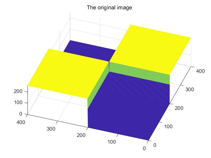
Refer to caption
Refer to caption
Refer to caption
Refer to caption
Figure 5.1: Fractional Riesz transform of order (π/4,π/4)𝜋4𝜋4(\pi/4,\pi/4) of a image.

As shown in Fig. 5.1, (a) is the original 2-dimensional grayscale image with 400 pixels ×\times 400 pixels; (c) is the 2-dimensional grayscale image after the Riesz transform of order (π/4,π/4)𝜋4𝜋4(\pi/4,\pi/4). In the continuous case, Fig. 5.1 (a) can be regarded as a function of 2superscript2\mathbb{R}^{2}

f(x1,x2)={0,(x1,x2)[0,200]2[200,400]2,255,otherwise.𝑓subscript𝑥1subscript𝑥2cases0subscript𝑥1subscript𝑥2superscript02002superscript2004002255otherwise.f(x_{1},x_{2})=\left\{\begin{array}[c]{ll}0,&(x_{1},x_{2})\in[0,200]^{2}\cup[200,400]^{2},\\ 255,&\textup{otherwise.}\end{array}\right.

Fig. 5.1 (b) and (d) are the 3-dimensional color graphs of f𝑓f and Rx1(π/4,π/4)fsuperscriptsubscript𝑅subscript𝑥1𝜋4𝜋4𝑓R_{x_{1}}^{(\pi/4,\pi/4)}f.

Recall that the fractional Fourier multiplier of the fractional Riesz transform Rj𝜶superscriptsubscript𝑅𝑗𝜶R_{j}^{\boldsymbol{\alpha}} is

mj𝜶(𝒖):=iu~j|𝒖~|.assignsuperscriptsubscript𝑚𝑗𝜶𝒖𝑖subscript~𝑢𝑗~𝒖m_{j}^{\boldsymbol{\alpha}}(\boldsymbol{u}):=-i\frac{\tilde{u}_{j}}{|\tilde{\boldsymbol{u}}|}.

Graphs (a) and (b) in Fig. 5.2 indicate that the fractional Riesz transform has the effect of amplitude reduction.

By comparing (c)/(e) and (d)/(f) in Fig. 5.2, as well as the real/imaginary part of αfsubscript𝛼𝑓\mathcal{F}_{\alpha}f and the imaginary/real part of 𝜶(Rj𝜶f)subscript𝜶superscriptsubscript𝑅𝑗𝜶𝑓\mathcal{F}_{\boldsymbol{\alpha}}(R_{j}^{\boldsymbol{\alpha}}f) accordingly, it can be seen that the fractional Riesz transform has the effect of phase shifting.

Above all, Fig. 5.2 shows that the fractional multiplier of Rj𝜶superscriptsubscript𝑅𝑗𝜶R_{j}^{\boldsymbol{\alpha}} is iu~j/|𝒖~|𝑖subscript~𝑢𝑗~𝒖-i\tilde{u}_{j}/|\tilde{\boldsymbol{u}}|, and thus, the fractional Riesz transform is not only a phase-shift converter but also an amplitude attenuator. This circumstance is quite different from that of the fractional multiplier of H𝜶subscript𝐻𝜶H_{\boldsymbol{\alpha}}, which is only a phase-shift converter with multiplier isgn((πα)u)𝑖sgn𝜋𝛼𝑢-i{\rm sgn}((\pi-\alpha)u).

Refer to caption
Refer to caption
Refer to caption
Refer to caption
Refer to caption
Refer to caption
Figure 5.2: Phase-shifting and amplitude-reducing effect of the fractional Riesz transform in the fractional Fourier domain of order 𝜶=(π/4,π/4)𝜶𝜋4𝜋4\boldsymbol{\alpha}=(\pi/4,\pi/4) on an image.

6 Application of the fractional Riesz transform in edge detection

Edge detection is a key technology in image processing. It is widely used in biometrics, image understanding, visual attention and other fields. Commonly used image feature extraction methods include the Roberts operator, Prewitt operator, Sobel operator, Laplacian operator and Canny operator. These algorithms extract features based on the gradient changes in the pixel amplitudes. In [16, 33, 34], the authors introduced the image edge detection methods based on the Riesz transform, which can avoid the influence of uneven illumination. Moreover, the Riesz transform has the characteristics of isotropy; therefore, the Riesz transform has more advantages in feature extraction. Based on the principle of Riesz transform edge detection, edge detection based on the fractional Riesz transform is proposed in this section.

When processing the two-dimensional signal f(𝒙)𝑓𝒙f(\boldsymbol{x}), the fractional Riesz transform of f(𝒙)𝑓𝒙f(\boldsymbol{x}) can be expressed as

(R1𝜶f)(𝒙)=cnp.v.e𝜶(𝒙)((e𝜶f)x1|𝒙|3)(𝒙),formulae-sequencesuperscriptsubscript𝑅1𝜶𝑓𝒙subscript𝑐𝑛pvsubscript𝑒𝜶𝒙subscript𝑒𝜶𝑓subscript𝑥1superscript𝒙3𝒙\displaystyle(R_{1}^{\boldsymbol{\alpha}}f)(\boldsymbol{x})=c_{n}\ {\rm p}.{\rm v}.\ e_{-\boldsymbol{\alpha}}(\boldsymbol{x})\left((e_{\boldsymbol{\alpha}}f)\ast\frac{x_{1}}{|\boldsymbol{x}|^{3}}\right)(\boldsymbol{x}), (6.1)
(R2𝜶f)(𝒙)=cnp.v.e𝜶(𝒙)((e𝜶f)x2|𝒙|3)(𝒙),formulae-sequencesuperscriptsubscript𝑅2𝜶𝑓𝒙subscript𝑐𝑛pvsubscript𝑒𝜶𝒙subscript𝑒𝜶𝑓subscript𝑥2superscript𝒙3𝒙\displaystyle(R_{2}^{\boldsymbol{\alpha}}f)(\boldsymbol{x})=c_{n}\ {\rm p}.{\rm v}.\ e_{-\boldsymbol{\alpha}}(\boldsymbol{x})\left((e_{\boldsymbol{\alpha}}f)\ast\frac{x_{2}}{|\boldsymbol{x}|^{3}}\right)(\boldsymbol{x}), (6.2)

or

(R1𝜶f)(𝒙)=[𝜶(iu1cscα1(u1cscα1)2+(u2cscα2)2(𝜶f)(𝒖))](𝒙),superscriptsubscript𝑅1𝜶𝑓𝒙delimited-[]subscript𝜶𝑖subscript𝑢1subscript𝛼1superscriptsubscript𝑢1subscript𝛼12superscriptsubscript𝑢2subscript𝛼22subscript𝜶𝑓𝒖𝒙\displaystyle(R_{1}^{\boldsymbol{\alpha}}f)(\boldsymbol{x})=\left[\mathcal{F}_{-\boldsymbol{\alpha}}\left(-i\frac{u_{1}\csc\alpha_{1}}{\sqrt{(u_{1}\csc\alpha_{1})^{2}+(u_{2}\csc\alpha_{2})^{2}}}(\mathcal{F}_{\boldsymbol{\alpha}}f)(\boldsymbol{u})\right)\right](\boldsymbol{x}), (6.3)
(R2𝜶f)(𝒙)=[𝜶(iu2cscα2(u1cscα1)2+(u2cscα2)2(𝜶f)(𝒖))](𝒙).superscriptsubscript𝑅2𝜶𝑓𝒙delimited-[]subscript𝜶𝑖subscript𝑢2subscript𝛼2superscriptsubscript𝑢1subscript𝛼12superscriptsubscript𝑢2subscript𝛼22subscript𝜶𝑓𝒖𝒙\displaystyle(R_{2}^{\boldsymbol{\alpha}}f)(\boldsymbol{x})=\left[\mathcal{F}_{-\boldsymbol{\alpha}}\left(-i\frac{u_{2}\csc\alpha_{2}}{\sqrt{(u_{1}\csc\alpha_{1})^{2}+(u_{2}\csc\alpha_{2})^{2}}}(\mathcal{F}_{\boldsymbol{\alpha}}f)(\boldsymbol{u})\right)\right](\boldsymbol{x}). (6.4)

For an image f(𝒙)𝑓𝒙f(\boldsymbol{x}), the monogenic signal is defined as the combination of f(𝒙)𝑓𝒙f(\boldsymbol{x}) and its fractional Riesz transform.

(p(𝒙),q1(𝒙),q2(𝒙))=(f(𝒙),(R1𝜶f)(𝒙),(R2𝜶f)(𝒙)).𝑝𝒙subscript𝑞1𝒙subscript𝑞2𝒙𝑓𝒙superscriptsubscript𝑅1𝜶𝑓𝒙superscriptsubscript𝑅2𝜶𝑓𝒙(p(\boldsymbol{x}),q_{1}(\boldsymbol{x}),q_{2}(\boldsymbol{x}))=(f(\boldsymbol{x}),(R_{1}^{\boldsymbol{\alpha}}f)(\boldsymbol{x}),(R_{2}^{\boldsymbol{\alpha}}f)(\boldsymbol{x})).

Therefore, the local amplitude value A(𝒙)𝐴𝒙A(\boldsymbol{x}), local orientation θ(𝒙)𝜃𝒙\theta(\boldsymbol{x}) and local phase P(𝒙)𝑃𝒙P(\boldsymbol{x}) in the monogenic signal in the image can be expressed as

{A(x)=p(𝒙)2+|q1(𝒙)|2+|q2(𝒙)|2θ(x)=tan1(|q2(𝒙)q1(𝒙)|)P(x)=tan1(p(𝒙)|q1(𝒙)|2+|q2(𝒙)|2).\displaystyle\left\{\begin{aligned} A(x)&=\sqrt{p(\boldsymbol{x})^{2}+|q_{1}(\boldsymbol{x})|^{2}+|q_{2}(\boldsymbol{x})|^{2}}\\ \theta(x)&=\tan^{-1}\left(\left|\frac{q_{2}(\boldsymbol{x})}{q_{1}(\boldsymbol{x})}\right|\right)\\ P(x)&=\tan^{-1}\left(\frac{p(\boldsymbol{x})}{\sqrt{|q_{1}(\boldsymbol{x})|^{2}+|q_{2}(\boldsymbol{x})|^{2}}}\right).\end{aligned}\right.

In this paper, we use the fractional Riesz transform in the form of (6.3) and (6.4) for algorithm design because the fractional Riesz transform can be decomposed into a combination of a FRFT, inverse FRFT and multiplier by the fractional multiplier Theorem 2.1. Because the FRFT and inverse FRFT have fast algorithms, compared with the form of (6.1) and (6.2), the computational complexity of the algorithm in the form of (6.3) and (6.4) is reduced. Thus, a faster and more efficient operation is realized.
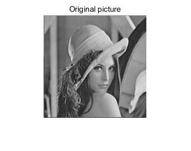
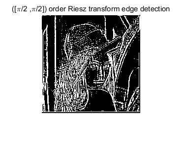
Refer to caption
Refer to caption
Figure 6.1: Original image and edge detection based on the fractional Riesz transform of order ([π/2,π/2])𝜋2𝜋2([\pi/2,\pi/2]) (i.e., the classical Riesz transform)
Refer to caption
Refer to caption
Refer to caption
Refer to caption
Refer to caption
Refer to caption
Figure 6.2: Extract the information of a specific position in the lateral direction of the image
Refer to caption
Refer to caption
Refer to caption
Refer to caption
Refer to caption
Refer to caption
Figure 6.3: Extract the information of specific position in the longitudinal direction of the image
Refer to caption
Refer to caption
Refer to caption
Refer to caption
Refer to caption
Refer to caption
Figure 6.4: Extract the information of the specific position in the main diagonal of the image
Refer to caption
Refer to caption
Refer to caption
Refer to caption
Refer to caption
Refer to caption
Figure 6.5: Extract the information of the specific position in the counter diagonal of the image

The simulation experiment will be conducted by using the classical Lena image ((a) in Fig. 6.1) as the test image. To better highlight the results of our simulation experiment, we choose an appropriate threshold value to binarize the images after the experiment in such a way that our experimental results show a more obvious effect. Graph (b) in Fig. 6.1 illustrates the result of edge detection based on the fractional Riesz transform of order ([π/2,π/2])𝜋2𝜋2([\pi/2,\pi/2]) (i.e., the classical Riesz transform).

Fig. 6.2 shows that when α1=π/2subscript𝛼1𝜋2\alpha_{1}=\pi/2 is fixed, if α2subscript𝛼2\alpha_{2} decreases from π/2𝜋2\pi/2 ((d), (e), (f) in Fig. 6.2), we extract information about the lateral up position. If α2subscript𝛼2\alpha_{2} increases from π/2𝜋2\pi/2 ((a), (b), (c) in Fig. 6.2), we extract information about the lateral down position. In conclusion, by fixed α1=π/2subscript𝛼1𝜋2\alpha_{1}=\pi/2, we can adjust α2subscript𝛼2\alpha_{2} to extract information on the specific position in the lateral direction.

Fig. 6.3 indicates that when α2=π/2subscript𝛼2𝜋2\alpha_{2}=\pi/2 is fixed and α1subscript𝛼1\alpha_{1} decreases from π/2𝜋2\pi/2 ((a), (b), (c) in Fig. 6.3), the longitudinal right position information is extracted. As α1subscript𝛼1\alpha_{1} increases from π/2𝜋2\pi/2 ((d), (e), (f) in Fig. 6.3), we extract the longitudinal left position information. In conclusion, when fixing α2=π/2subscript𝛼2𝜋2\alpha_{2}=\pi/2, we can extract information of the specific longitudinal positions by adjusting α1subscript𝛼1\alpha_{1}.

Fig. 6.4 shows that when α1subscript𝛼1\alpha_{1} and α2subscript𝛼2\alpha_{2} increase or decrease the same size from π/2𝜋2\pi/2, the information on the specific direction in the main diagonal is extracted.

Fig. 6.5 indicates that when α1subscript𝛼1\alpha_{1} increases from π/2𝜋2\pi/2 and α2subscript𝛼2\alpha_{2} decreases from π/2𝜋2\pi/2 by the same size, the information on the specific direction in the antidiagonal is extracted.

The preceding simulation provides a new edge detection tool based on the the fractional Riesz transform, that extracts both global features and local features of images. This numerical implementation confirms the belief expressed in [26] that amplitude, phase, and direction information can be simultaneously extracted by controlling the order of the fractional Riesz transform. We predict that very comprehensive analysis and processing of multidimensional signals, such as images, videos, 3D meshes and animations, can be achieved via the fractional Riesz transforms.

7 Conclusions

In this paper, we introduced the fractional Riesz transform and give the corresponding fractional multiplier theorem and its applications in partial differential equations. We also studied properties of chirp singular integral operators, chirp Hardy spaces and chirp BMO spaces. We used the fractional Riesz transforms in concrete applications in edge detection with surprisingly good results. Our experiments indicate that edge detection can extract local information in any direction by adjusting the order of the fractional Riesz transform. The algorithm complexity of the fractional Riesz transform in the form of (6.3) and (6.4) is reduced compared with the fractional Riesz transform of (6.1) and (6.2).

References

References