Analytical impedance of oxygen transport in the channel and gas diffusion layer of a PEM fuel cell

Abstract

Analytical model for impedance of oxygen transport in the gas–diffusion layer (GDL) and cathode channel of a PEM fuel cell is developed. The model is based on transient oxygen mass conservation equations coupled to the proton current conservation equation in the catalyst layer. Analytical formula for the “GDL+channel” impedance is derived assuming that the oxygen and proton transport in the cathode catalyst layer (CCL) are fast. In the Nyquist plot, the resulting impedance consists of two arcs describing oxygen transport in the air channel (low–frequency arc) and in the GDL. The characteristic frequency of GDL arc depends on the CCL thickness: large CCL thickness strongly lowers this frequency. At small CCL thickness, the high–frequency feature on the arc shape forms. This effect is important for identification of peaks in distribution of relaxation times spectra of low–Pt PEMFCs.

I Introduction

Electrochemical impedance spectroscopy (EIS) provides invaluable information on transport properties of PEM fuel cell in a current production mode, without interruption of cell functioning[1]. Not surprisingly, EIS of PEM fuel cells is a rapidly growing field[2]. Understanding impedance spectra requires modeling. Strong criticism of equivalent circuit approach has been published by Macdonald in his seminal paper[3] and in recent years, physics–based models for PEMFC impedance tend to replace equivalent circuit modeling (see recent reviews of Tang et al. [2] and Huang et al. [4]).

Every transport and kinetic process in a PEM fuel cell has its own resonance frequency. If these frequencies do not overlap, one could identify them using the distribution of relaxation times (DRT) technique[5, 6, 7]. In addition, DRT analysis of impedance spectra returns the contribution of every process into the total differential resistance of the cell. However, correct identification of DRT peaks is a non–trivial task requiring modeling and experimental work. Analytical models predicting characteristic frequencies of oxygen transport processes in the cell could be very helpful in this respect.

Oxygen reduction reaction (ORR) is usually responsible for a large part of potential loss in a PEMFC. Oxygen is transported to the catalyst sites through the cathode channel and gas–diffusion layer; both the transport processes have their signatures in the EIS spectra. After pioneering experimental work of Schneider et al. [8, 9], Kulikovsky and Shamardina[10, 11], Maranzana et al. [12] and Chevalier et al. [13] developed numerical and analytical models incorporating channel impedance. Formulas for pure channel impedance have been obtained[13, 14] assuming fast oxygen transport through the GDL and cathode catalyst layer (CCL). However, the coupling between the channel and GDL impedance remained poorly understood. Recently, Cruz–Manzo and Greenwood reported analytical model for the GDL+channel impedance[15]. However, their result missing important effect of double layer charging on this impedance, as discussed below.

In this work, we develop analytical model for the GDL+channel impedance $Z_{gdlc}$ in a PEM fuel cell. Assuming fast oxygen and proton transport in the CCL, analytical expression for $Z_{gdlc}$ is derived. We show that for typical PEMFC parameters, the Nyquist spectrum of $Z_{gdlc}$ consists of two arcs corresponding to oxygen transport in the channel and GDL. GDL impedance differs from the Warburg finite–length impedance due to “non–Warburg” factor depending on the superficial double layer capacitance of the electrode. For typical PEMFC parameters, the characteristic frequency $f_{gdl}$ of the GDL impedance $Z_{gdl}$ is close to the Warburg finite–length frequency; however, for larger CCL thickness typical for non–Pt cells, the non–Warburg factor strongly lowers $f_{gdl}$. In the opposite limit of small catalyst layer thickness, a high–frequency feature on the shape of imaginary part of $Z_{gdl}$ vs frequency forms. Analysis shows that the channel impedance also depends on the double layer capacitance meaning that impedance of all oxygen transport medias in the PEMFC “feel” double layer capacitance of the electrode where the oxygen is transported to. The goal of this paper is to clarify the situation with oxygen transport impedance in the GDL and channel after interesting and useful, but incomplete and rather difficult for understanding work of Cruz-Manzo and Greenwood[15].

II Model

Schematic of the cell with the straight cathode channel is shown in Figure 1. Our main goal here is analysis of impedance of the GDL+channel oxygen transport system. To simplify the model and to separate the GDL+channel impedance from impedance of oxygen transport in the CCL, we will assume that the latter transport is fast. In addition, for simplicity we will assume that the proton transport in the CCL is also fast. The characteristic frequency of proton transport in the CCL is much higher than the other frequencies in the system and hence this assumption does not affect low– and medium–frequency impedances which are of primary interest in this work.

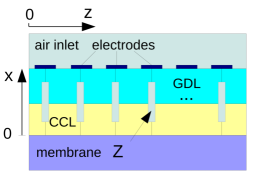
Figure 1: Schematic of the segmented cell cathode side with the straight channel and the system of coordinates. $Z$ stands for local impedance depending on the distance along the channel coordinate $z$.

II.1 Proton charge conservation equation

The proton charge conservation equation reads

$$C_{dl}\dfrac{\partial{\eta}}{\partial{t}}+\dfrac{\partial{j}}{\partial{x}}=-i_{*}\left(\dfrac{c}{c_{h}^{in}}\right)\exp\left(\dfrac{\eta}{b}\right)$$ (1)

where $C_{dl}$ is the volumetric double layer capacitance (F cm^-3), $\eta$ is the positive by convention ORR overpotential, $j$ is the local proton current density in the CCL, $x$ is coordinate through the cell cathode counted from the membrane, $i_{*}$ is the volumetric exchange current density (A cm^-3), $c$ is the local oxygen concentration, $c_{h}^{in}$ is the reference oxygen concentration, and $b$ is the ORR Tafel slope.

Since proton and oxygen transport in the CCL are fast, $\eta$ and $c$ are nearly independent of $x$. Integrating Eq.(1) over $x$ from 0 to the CCL thickness $l_{t}$ we come to

$$C_{dl}l_{t}\dfrac{\partial{\eta_{0}}}{\partial{t}}-j_{0}=-i_{*}l_{t}\left(\dfrac{c_{1}}{c_{h}^{in}}\right)\exp\left(\dfrac{\eta_{0}}{b}\right)$$ (2)

where $\eta_{0}$ is the ORR overpotential at the membrane surface, $j_{0}$ is the local cell current density, and $c_{1}$ is the oxygen concentration at the CCL/GDL interface.

To simplify calculations, we introduce dimensionless variables

$$\tilde{t}=\dfrac{t}{t_{*}},\quad\tilde{x}=\dfrac{x}{l_{t}},\quad\tilde{z}=\dfrac{z}{L},\quad\tilde{c}=\dfrac{c}{c_{h}^{in}},\quad\tilde{j}=\dfrac{j}{i_{*}l_{t}},\\ \tilde{\eta}=\dfrac{\eta}{b},\quad\tilde{D}_{b}=\dfrac{4FD_{b}c_{h}^{in}}{i_{*}l_{t}^{2}},\quad\tilde{l}_{b}=\dfrac{l_{b}}{l_{t}},\\ \tilde{\omega}=\omega t_{*},\quad\tilde{Z}=\dfrac{Zi_{*}l_{t}}{b}$$ (3)

where

$$t_{*}=\dfrac{C_{dl}b}{i_{*}},$$ (4)

is the characteristic time of double layer charging, $z$ is the coordinate along the cathode channel, $L$ is the channel length, $D_{b}$ is the oxygen diffusion coefficient in the GDL, $l_{b}$ is the GDL thickness, $\omega$ is the angular frequency of the applied AC signal, and $Z$ is the local impedance.

With the dimensionless variables (3), Eq.(2) takes the form

$$\dfrac{\partial{\tilde{\eta}_{0}}}{\partial{\tilde{t}}}-\tilde{j}_{0}=-\tilde{c}_{1}{{\rm e}^{\tilde{\eta}_{0}}}$$ (5)

Substituting Fourier–transforms

$$\begin{split}&\tilde{\eta}_{0}=\tilde{\eta}^{0}+\tilde{\eta}^{1}(\tilde{\omega})\exp({\rm i}\tilde{\omega}\tilde{t})\\ &\tilde{j}_{0}=\tilde{j}^{0}+\tilde{j}^{1}(\tilde{\omega})\exp({\rm i}\tilde{\omega}\tilde{t})\\ &\tilde{c}_{1}=\tilde{c}_{1}^{0}+\tilde{c}_{1}^{1}(\tilde{\omega})\exp({\rm i}\tilde{\omega}\tilde{t})\end{split}$$ (6)

into Eq.(5), expanding exponent in Taylor series, neglecting term with the perturbations product, and subtracting the static equation, we get equation relating the small perturbation amplitudes $\tilde{\eta}^{1}$, $\tilde{j}^{1}$ and $\tilde{c}_{1}^{1}$ in the $\tilde{\omega}$–space:

$$\tilde{j}^{1}={\rm i}\tilde{\omega}\tilde{\eta}^{1}+{{\rm e}^{\tilde{\eta}_{0}}}\left(\tilde{c}_{1}^{1}+\tilde{c}_{1}^{0}\tilde{\eta}^{1}\right).$$ (7)

Here, the superscripts 0 and 1 mark the static variables and the small perturbation amplitudes, respectively. Local cathode side impedance at a distance $\tilde{z}$ from the channel inlet is given by

$$\tilde{Z}=\dfrac{\tilde{\eta}^{1}}{\tilde{j}^{1}}$$ (8)

Dividing Eq.(7) by $\tilde{j}^{1}$, we obtain equation for $\tilde{Z}$:

$$1=\left({\rm i}\tilde{\omega}+\tilde{c}_{1}^{0}{{\rm e}^{\tilde{\eta}_{0}}}\right)\tilde{Z}+{{\rm e}^{\tilde{\eta}_{0}}}\dfrac{\tilde{c}_{1}^{1}}{\tilde{j}^{1}}$$ (9)

Suppose that the perturbation of oxygen concentration is zero: $\tilde{c}_{1}^{1}=0$. Physically, this is equivalent to fast oxygen transport in all transport medias of the cathode side, including channel. Solution to Eq.(9) is then

$$\tilde{Z}_{f}=\dfrac{1}{{\rm i}\tilde{\omega}+\tilde{c}_{1}^{0}{{\rm e}^{\tilde{\eta}_{0}}}},$$ (10)

which is impedance of a parallel $RC$–circuit, where the term ${\rm i}\tilde{\omega}$ in denominator describes contribution of the double layer capacitance and $\tilde{c}_{1}^{0}{{\rm e}^{\tilde{\eta}_{0}}}$ is the inverse faradaic resistivity of the catalyst layer.

The static oxygen concentration $\tilde{c}_{1}^{0}$ is related to the channel concentration $\tilde{c}_{h}^{0}$ as

$$\tilde{c}_{1}^{0}=\tilde{c}_{h}^{0}\left(1-\dfrac{\tilde{j}^{0}}{\tilde{j}_{\lim}}\right)$$ (11)

where

$$j_{\lim}=\dfrac{4FD_{b}c_{h}^{0}}{l_{b}}$$ (12)

is the local limiting current density due to oxygen transport in the GDL. Eq.(11) is solution of the static version of equation for oxygen transport in the GDL, see Eq.(18) below. The concentration $\tilde{c}_{h}^{0}$ varies along the channel; numerical model[16] shows that unless the mean cell current density is small, this variation to a good approximation is linear:

$$\tilde{c}_{h}^{0}\simeq 1-\dfrac{\tilde{z}}{\lambda}$$ (13)

Note that Eq.(13) is an approximation the exact shape of $\tilde{c}_{h}^{0}(\tilde{z})$ should be calculated using a numerical model[17, 16].

To simplify calculations, we will ignore the factor $1-{\tilde{j}^{0}}/{\tilde{j}_{\lim}}$ in Eq.(11), assuming that $j_{\lim}$ is large and the variation of static oxygen concentration across the GDL is negligible. With this, Eqs.(7), (9) transform to

$$\tilde{j}^{1}={\rm i}\tilde{\omega}\tilde{\eta}^{1}+{{\rm e}^{\tilde{\eta}_{0}}}\left(\tilde{c}_{1}^{1}+\left(1-\dfrac{\tilde{z}}{\lambda}\right)\tilde{\eta}^{1}\right)$$ (14)

$$1=\left({\rm i}\tilde{\omega}+{{\rm e}^{\tilde{\eta}_{0}}}\left(1-\dfrac{\tilde{z}}{\lambda}\right)\right)\tilde{Z}+{{\rm e}^{\tilde{\eta}_{0}}}\dfrac{\tilde{c}_{1}^{1}}{\tilde{j}^{1}}$$ (15)

As discussed above, the non–faradaic oxygen transport contributions to local impedance gives the term with $\tilde{c}_{1}^{1}$. In order to calculate $\tilde{c}_{1}^{1}$, we need to consecutively solve equations for oxygen transport in the GDL and channel, as discussed in the next section.

For further references we need a total faradaic impedance $\tilde{Z}_{f,tot}$ of the cathode, taking into account variation of oxygen concentration along the channel. Suppose that the cell is divided into $N\to\infty$ virtual segments. Local current in each segment flows in the through–plane direction, hence local faradaic impedances are connected in parallel. Thus, $\tilde{Z}_{f,tot}$ is given by

$$\tilde{Z}_{f,tot}=\left(\int_{0}^{1}\dfrac{d\tilde{z}}{\tilde{Z}_{f}}\right)^{-1}$$ (16)

Electron conductivity of the cell components is assumed to be large and hence $\tilde{\eta}^{0}$ is independent of the coordinate $\tilde{z}$. Substituting Eq.(13) into Eq.(10), we get the local faradaic impedance $\tilde{Z}_{f}(\tilde{z})$. Calculating integral, from Eq.(16) we find

$$\tilde{Z}_{f,tot}=\dfrac{1}{{\rm i}\tilde{\omega}+\left(1-\dfrac{1}{2\lambda}\right){{\rm e}^{\tilde{\eta}_{0}}}}$$ (17)

II.2 Oxygen transport in the GDL

Oxygen transport in the gas–diffusion layer is described by the diffusion equation

$$\dfrac{\partial{c_{b}}}{\partial{t}}-D_{b}\dfrac{\partial^{2}{c_{b}}}{\partial{x}^{2}}=0,\quad\left.D_{b}\dfrac{\partial{c_{b}}}{\partial{x}}\right|_{x=l_{t}+}=\dfrac{j_{0}}{4F},\\ c_{b}(l_{t}+l_{b})=c_{h},$$ (18)

where $c_{b}$ is the oxygen concentration in the GDL and $c_{h}$ is the oxygen concentration in channel. The left boundary condition for Eq.(18) means that the oxygen flux on the GDL side of the CCL/GDL interface equals the local current density in the cell. This condition agrees with the assumption of fast oxygen transport in the CCL.

With the dimensionless variables Eq.(3), Eq.(18) takes the form

$$\mu^{2}\dfrac{\partial{\tilde{c}_{b}}}{\partial{\tilde{t}}}-\tilde{D}_{b}\dfrac{\partial^{2}{\tilde{c}_{b}}}{\partial{\tilde{x}}^{2}}=0,\quad\left.\tilde{D}_{b}\dfrac{\partial{\tilde{c}_{b}}}{\partial{\tilde{x}}}\right|_{\tilde{x}=1+}=\tilde{j}_{0},\\ \tilde{c}_{b}(1+\tilde{l}_{b})=\tilde{c}_{h},$$ (19)

where the dimensionless parameter $\mu$ is given by

$$\mu=\sqrt{\dfrac{4Fc_{h}^{in}}{C_{dl}b}}.$$ (20)

Eq.(19) is linear and hence the equation for the small perturbation amplitude $\tilde{c}_{b}^{1}$ is

$$\tilde{D}_{b}\dfrac{\partial^{2}{\tilde{c}_{b}^{1}}}{\partial{\tilde{x}}^{2}}={\rm i}\tilde{\omega}\mu^{2}\tilde{c}_{b}^{1},\quad\left.\tilde{D}_{b}\dfrac{\partial{\tilde{c}_{b}^{1}}}{\partial{\tilde{x}}}\right|_{\tilde{x}=1+}=\tilde{j}^{1},\\ \tilde{c}_{b}^{1}\left(1+\tilde{l}_{b}\right)=\tilde{c}_{h}^{1}$$ (21)

where $\tilde{c}_{h}^{1}$ is the oxygen perturbation in channel (see below).

Solution to Eq.(21) is

$$\tilde{c}_{b}^{1}=-\dfrac{\tilde{j}^{1}\sinh\left(\mu\sqrt{{\rm i}\tilde{\omega}/\tilde{D}_{b}}\,\left(1+\tilde{l}_{b}-\tilde{x}\right)\right)}{\mu\sqrt{{\rm i}\tilde{\omega}\tilde{D}_{b}}\cosh\left(\mu\tilde{l}_{b}\sqrt{{\rm i}\tilde{\omega}/\tilde{D}_{b}}\right)}\\ +\dfrac{\tilde{c}_{h}^{1}\cosh\left(\,\mu\sqrt{{\rm i}\tilde{\omega}/\tilde{D}_{b}}(1-\tilde{x})\right)}{\cosh\left(\mu\tilde{l}_{b}\sqrt{{\rm i}\tilde{\omega}/\tilde{D}_{b}}\right)}$$ (22)

Setting here $\tilde{x}=1$, we get the perturbation amplitude of oxygen concentration at the CCL/GDL interface $\tilde{c}_{b}^{1}(1)=\tilde{c}_{1}^{1}$

$$\tilde{c}_{1}^{1}=-\dfrac{\tilde{j}^{1}\tanh\left(\phi\right)}{\psi}+\dfrac{\tilde{c}_{h}^{1}}{\cosh\left(\phi\right)}$$ (23)

where $\phi$ and $\psi$ are auxiliary dimensonless parameters

$$\begin{split}&\phi=\mu\tilde{l}_{b}\sqrt{{\rm i}\tilde{\omega}/\tilde{D}_{b}}\\ &\psi=\mu\sqrt{{\rm i}\tilde{\omega}\tilde{D}_{b}}\end{split}$$ (24)

II.3 Oxygen transport in channel

To a good approximation, oxygen mass transport in the channel can be described by the 1d + 1d plug flow equation:

$$\dfrac{\partial{c_{h}}}{\partial{t}}+v\dfrac{\partial{c_{h}}}{\partial{z}}=-\left.\dfrac{D_{b}}{h}\dfrac{\partial{c_{b}}}{\partial{x}}\right|_{x=l_{t}+l_{b}}$$ (25)

where $h$ is the channel depth. The right side of Eq.(25) is the oxygen diffusive flux in the GDL at the channel/GDL interface representing oxygen “sink” from the channel.

With the dimensionless variables (3), Eq.(25) reads

$$\xi^{2}\dfrac{\partial{\tilde{c}_{h}}}{\partial{\tilde{t}}}+\lambda\tilde{J}\dfrac{\partial{\tilde{c}_{h}}}{\partial{\tilde{z}}}=-\left.\tilde{D}_{b}\dfrac{\partial{\tilde{c}_{b}}}{\partial{\tilde{x}}}\right|_{\tilde{x}=1+\tilde{l}_{b}}$$ (26)

where $\tilde{J}$ is the mean current density in the cell

$$\tilde{J}=\int_{0}^{1}\tilde{j}_{0}d\tilde{z},$$ (27)

$\xi$ is the dimensionless parameter, and $\lambda$ is the stoichiometry of air flow

$$\xi=\sqrt{\dfrac{4Fhc_{h}^{in}}{C_{dl}l_{t}b}},\quad\lambda=\dfrac{4Fhvc_{h}^{in}}{LJ}.$$ (28)

Eq.(26) is linear and we can immediately write down equation for the perturbation amplitude $\tilde{c}_{h}^{1}$:

$$\lambda\tilde{J}\dfrac{\partial{\tilde{c}_{h}^{1}}}{\partial{\tilde{z}}}=-{\rm i}\tilde{\omega}\xi^{2}\tilde{c}_{h}^{1}-\left.\tilde{D}_{b}\dfrac{\partial{\tilde{c}_{b}^{1}}}{\partial{\tilde{x}}}\right|_{\tilde{x}=1+\tilde{l}_{b}}$$ (29)

Differentiating Eq.(22), we find the flux $\tilde{D}_{b}{\partial{\tilde{c}_{b}^{1}}}/{\partial{\tilde{x}}}|_{\tilde{x}=1+\tilde{l}_{b}}$ and Eq.(29) takes the form

$$\lambda\tilde{J}\dfrac{\partial{\tilde{c}_{h}^{1}}}{\partial{\tilde{z}}}=-{\rm i}\tilde{\omega}\xi^{2}\tilde{c}_{h}^{1}-\tilde{j}^{1}\cosh\left(\phi\right)^{-1}-\tilde{c}_{h}^{1}\psi\,\tanh\left(\phi\right),\\ \tilde{c}_{h}^{1}(0)=0$$ (30)

where $\tilde{j}^{1}$ is a function of coordinate $\tilde{z}$ and of $\tilde{c}_{h}^{1}$. To find the explicit dependence $\tilde{j}^{1}(\tilde{z})$ we substitute (23) into Eq.(14); solving the resulting equation for $\tilde{j}^{1}$ we get

$$\tilde{j}^{1}=\left(\dfrac{{{\rm e}^{\tilde{\eta}_{0}}}\tanh\left(\phi\right)}{\psi}+1\right)^{-1}\\ \times\left(\left({\rm i}\tilde{\omega}+{{\rm e}^{\tilde{\eta}_{0}}}\left(1-\dfrac{\tilde{z}}{\lambda}\right)\right)\tilde{\eta}^{1}+\dfrac{{{\rm e}^{\tilde{\eta}_{0}}}\tilde{c}_{h}^{1}}{\cosh(\phi)}\right)$$ (31)

II.4 Solution procedure and total cathode impedance

Substituting $\tilde{j}^{1}$, Eq.(31), into Eq.(30) and solving the resulting equation we find the amplitude of oxygen concentration perturbation along the channel

$$\tilde{c}_{h}^{1}(\tilde{z})=\dfrac{\tilde{\eta}^{1}}{B}\left(\left(\dfrac{A\lambda\tilde{J}}{B}+C\right)\left(\exp\left(\dfrac{B\tilde{z}}{\lambda\tilde{J}}\right)-1\right)-A\tilde{z}\right)$$ (32)

where the independent of $\tilde{z}$ coefficients $A$, $B$ and $C$ are given by

$$A=\dfrac{\psi{{\rm e}^{\tilde{\eta}_{0}}}}{\lambda\cosh(\phi)\left(\psi+{{\rm e}^{\tilde{\eta}_{0}}}\tanh(\phi)\right)}$$ (33)

$$B=-{\rm i}\tilde{\omega}\xi^{2}-\psi\tanh(\phi)-\dfrac{\lambda A}{\cosh(\phi)}$$ (34)

$$C=-\dfrac{\psi\left({\rm i}\tilde{\omega}+{{\rm e}^{\tilde{\eta}_{0}}}\right)}{\cosh(\phi)\left(\psi+{{\rm e}^{\tilde{\eta}_{0}}}\tanh(\phi)\right)}$$ (35)

Setting in Eq.(32) $\tilde{\eta}^{1}=\tilde{Z}\tilde{j}^{1}$ and using the result in Eq.(23) we get a formula for $\tilde{c}_{1}^{1}$, which linearly depends on $\tilde{Z}$. Substituting this $\tilde{c}_{1}^{1}$ into Eq.(15), we obtain a linear algebraic equation for local impedance $\tilde{Z}$. Solving this equation, we find local impedance, which includes faradaic and oxygen transport in the channel and GDL processes

$$\tilde{Z}(\tilde{z})=\dfrac{B^{2}}{D_{loc}}\left(\cosh(\phi)+\dfrac{{{\rm e}^{\tilde{\eta}_{0}}}\sinh(\phi)}{\psi}\right)$$ (36)

where

$$D_{loc}={{\rm e}^{\tilde{\eta}_{0}}}\left(\lambda\tilde{J}A+BC\right)\left(\exp\left(\dfrac{B\tilde{z}}{\lambda\tilde{J}}\right)-1\right)\\ +B^{2}\left({\rm i}\tilde{\omega}+{{\rm e}^{\tilde{\eta}_{0}}}\left(1-\dfrac{\tilde{z}}{\lambda}\right)\right)\cosh(\phi)-{{\rm e}^{\tilde{\eta}_{0}}}BA\tilde{z}.$$ (37)

Note that $D_{loc}$ contains complex exponent $\exp\left({B\tilde{z}}/({\lambda\tilde{J}})\right)$ leading to oscillations of $\tilde{Z}$ along the channel coordinate $\tilde{z}$ (Ref.[11]).

The total cathode side impedance is given by

$$\tilde{Z}_{tot}=\left(\int_{0}^{1}\dfrac{d\tilde{z}}{\tilde{Z}}\right)^{-1}$$ (38)

Calculation of integral leads to

$$\tilde{Z}_{tot}=\dfrac{\lambda B^{3}}{D_{tot}}\left(\cosh(\phi)+\dfrac{{{\rm e}^{\tilde{\eta}_{0}}}\sinh(\phi)}{\psi}\right)$$ (39)

where

$$D_{tot}=\lambda^{2}\tilde{J}{{\rm e}^{\tilde{\eta}_{0}}}\left(\lambda\tilde{J}A+BC\right)\left(\exp\left(\dfrac{B}{\lambda\tilde{J}}\right)-1\right)\\ +\left(({\rm i}\tilde{\omega}+{{\rm e}^{\tilde{\eta}_{0}}})\lambda-{{\rm e}^{\tilde{\eta}_{0}}}/2\right)B^{3}\cosh(\phi)\\ -\lambda{{\rm e}^{\tilde{\eta}_{0}}}B\left(\lambda\tilde{J}A+B(A/2+C)\right).$$ (40)

The closed form of integral in Eq.(38) is a key point leading to analytical formula for $\tilde{Z}_{tot}$. At high frequencies of the AC signal, $\tilde{c}_{h}^{1}$ and local impedance $\tilde{Z}$ are rapidly oscillating functions of $\tilde{z}$, which requires a lot of steps in numerical solution of Eq.(29) and makes it difficult numerical calculation of Eq.(38). Analytical result for integral in Eq.(38) solves the problem.

III Results and Discussion

Equations of the previous Section contain mean current density in the cell $\tilde{J}$ and the total static potential loss (overpotential) $\tilde{\eta}^{0}$. These parameters are related by the polarization curve, which could be obtained from solution of the static version of equations (1), (18) and (25). The solution is Tafel–like equation corrected for the finite flow stoichiometry $\lambda$ (Ref.[19]):

$$-\lambda\ln\left(1-\dfrac{1}{\lambda}\right)\tilde{J}={{\rm e}^{\tilde{\eta}_{0}}}$$ (41)

Note that Eq.(41) does not include the effect of cell ohmic resistivity. If experimental polarization curve is available, an IR–corrected numerical relation between $\tilde{\eta}^{0}$ and $\tilde{J}$ could be used instead of Eq.(41). A more accurate numerical approximation for the polarization curve could be obtained using the model[17, 16].

Eq.(41) allows us to eliminate ${{\rm e}^{\tilde{\eta}_{0}}}$ from Eq.(39). Nyquist spectra of total cathode side impedance $Z_{tot}$ for the parameters listed in Table 1, the mean cell current density $J=0.5$ A cm^-2 and several stoichiometries of the air flow are shown in Figure 2a. Figure 2b shows the frequency dependence of $\operatorname{Im}\left(Z_{tot}\right)$. As can be seen, the impedance consists of three arcs, of which the low–frequency (LF) one strongly depends on $\lambda$ (Figure 2a). In the pioneering experiments of Schneider et al. this arc has been associated with the oxygen transport in channel[8, 9]. The LF arc vanishes as $\lambda\to\infty$ (Figures 2a,b).

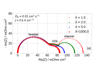
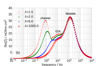
Figure 2: (a) Nyquist spectra of the total cathode side impedance, Eq.(39), for the indicated air flow stoichiometries $\lambda$. The cell current density is 0.5 A cm^-2. (b) Frequency dependence of imaginary part of impedance in (a).

The medium–frequency (MF) arc in Figure 2a represents oxygen transport in the GDL. This arc is not fully seen due to masking effect of the third, high–frequency (HF) faradaic arc (Figure 2). To emphasize the GDL arc, we subtract the total faradaic impedance (17) from the total cathode impedance, Eq.(39). This leads to the GDL+channel impedance $\tilde{Z}_{gdlc}$:

$$\tilde{Z}_{gdlc}=\tilde{Z}_{tot}-\dfrac{1}{{\rm i}\tilde{\omega}+\left(1-\dfrac{1}{2\lambda}\right){{\rm e}^{\tilde{\eta}_{0}}}}$$ (42)

Nyquist spectra of Eq.(42) for the same parameters exhibit two arcs; now the left, GDL arc is fully resolved (Figure 3a). Frequency dependence of $\operatorname{Im}\left(Z_{gdlc}\right)$ is shown in Figure 3b. Two peaks in Figure 3b correspond to the channel and GDL arcs in Figure 3a. At low stochiometry of the air flow, the GDL arc is located at the right “wing” of the channel arc; the latter contributes to imaginary part of the GDL impedance (Figure 3b). However, as $\lambda$ increases, the channel arc vanishes and only GDL arc is left (the curves for $\lambda=1000$ in Figures 3a,b).

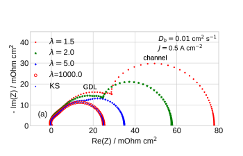
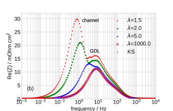
Figure 3: (a) Nyquist spectra of the GDL+channel impedance, Eq.(42), for the indicated air flow stoichiometries $\lambda$. The cell current density is $J=0.5$ A cm^-2. KS marks the spectrum of Eq.(44). (b) Frequency dependence of imaginary part of impedance in (a).

GDL thickness $l_{b}$, cm	0.023
Catalyst layer thickness $l_{t}$, cm	$10\cdot 10^{-4}$ (10 $\mu$m)
ORR Tafel slope $b$, mV	30
Double layer capacitance $C_{dl}$, F cm-3	20
GDL oxygen diffusivity $D_{b}$, cm2 s-1	0.01
Cell current density $j_{0}$, A cm-2	0.1
Pressure	Standard
Cell temperature $T$, K	273 + 80
Aur flow stoichiometry $\lambda$	2.0

Table 1: The base–case cell parameters used in calculations.

Equation for GDL impedance in the limit of infinite air flow stoichiometry has been derived by Kulikovsky and Shamardina[11]. In the notations of this work, Eq.(36) of Ref.[11] is

$$\tilde{Z}_{gdl}=\dfrac{\tanh\left(\mu\tilde{l}_{b}\sqrt{{\rm i}\tilde{\omega}/\tilde{D}_{b}}\right)}{\mu\sqrt{{\rm i}\tilde{\omega}\tilde{D}_{b}}\left(1-\tilde{J}\tilde{l}_{b}/\tilde{D}_{b}\right)\left(1+{\rm i}\tilde{\omega}/\tilde{J}\right)}$$ (43)

The frequency–independent factor $(1-\tilde{J}\tilde{l}_{b}/\tilde{D}_{b})$ in denominator describes the growth of static resistivity upon approaching the limiting current density $\tilde{D}_{b}/\tilde{l}_{b}$ due to oxygen transport in the GDL. In this work, we assume that the limiting current is large and the factor $(1-\tilde{J}\tilde{l}_{b}/\tilde{D}_{b})$ can be replaced by unity. With this, Eq.(43) simplifies to

$$\tilde{Z}_{gdl}=\dfrac{\tanh\left(\mu\tilde{l}_{b}\sqrt{{\rm i}\tilde{\omega}/\tilde{D}_{b}}\right)}{\mu\sqrt{{\rm i}\tilde{\omega}\tilde{D}_{b}}\left(1+{\rm i}\tilde{\omega}/\tilde{J}\right)}$$ (44)

Eq.(44) can be directly obtained from Eq.(42) by passing to the limit $\lambda\to\infty$. The spectrum of Eq.(44) (KS–spectrum) is shown in Figures 3a,b by small blue dots. As expected, the spectrum of Eq.(42) for $\lambda=1000$ (red open circles, Figure 3a,b) is practically indistinguishable with the spectrum of Eq.(44).

Of particular interest is the “non–Warburg” factor $(1+{\rm i}\tilde{\omega}/\tilde{J})$ in denominator of Eq.(44). Without this factor, Eq.(44) is equivalent to the Warburg finite–length impedance[1]. “Non–Warburg” shape of the GDL Nyquist arc (HF part of this arc looks like an elephant’s trunk, Figure 3a) is due to the effect of charging double layer capacitance in the CCL[11]. In other words, the GDL impedance “feels” the double layer capacitance of the attached CCL, since CCL provides a boundary condition for oxygen transport through the GDL. Similar capacitive correction to the classic Warburg impedance has been discussed by Barbero[20] in the context of Poisson–Nernst–Plank model for the planar electrode. It is worth noting a detailed study of the effect of non–capacitive boundary conditions on Warburg impedance published recently by Huang[21].

The non–Warburg factor $(1+{\rm i}\tilde{\omega}/\tilde{J})$ in Eq.(44) leads to important effects. In the dimension form, ${\rm i}\tilde{\omega}/\tilde{J}={\rm i}\omega C_{dl}l_{t}b/J$, i.e., this factor includes the superficial double layer capacitance $C_{dl}l_{t}$ (F cm^-2) of the CCL. Under constant volumetric DL capacitance $C_{dl}$ (F cm^-3), this results in dependence of the GDL spectrum on the catalyst layer thickness $l_{t}$. Figure 4 shows that with typical for Pt/C–based PEMFCs CCL thickness in the range of 10 $\mu$m to 1 $\mu$m, the effect of non-Warburg factor on the characteristic frequency $f_{gdl}$ of GDL spectrum is small and $f_{gdl}$ is close to the Warburg finite–length frequency $f_{W}$:

$$f_{W}=\dfrac{2.54D_{b}}{2\pi l_{b}^{2}}$$ (45)

However, for CCL thickness on the order of 100 $\mu$m typical for cells with non–Pt catalysts[22], the non–Warburg factor strongly shifts the frequency $f_{gdl}$ to lower values (Figure 4). This may lead to partial overlapping of the GDL and channel peaks of the respective imaginary parts (cf. Figure 3b, the curve for $\lambda=5$). Figure 4 also shows that with the decrease in CCL thickness, the width of the GDL peak increases. Moreover, at low $l_{t}$, the non–Warburg factor leads to formation of a distinct high–frequency feature in the spectrum (Figure 4). The effects in Figure 4 are particularly important for identification of DRT peaks in the high– and low–Pt PEM fuel cell spectra. The thickness of a low–Pt CCL is typically three to four times less than the high–Pt CCL thickness, while the volumetric $C_{dl}$ in both types of cells is the same.

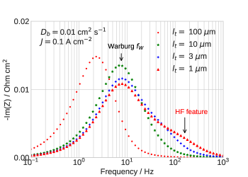
Figure 4: Frequency dependence of imaginary part of the GDL impedance, Eq.(44), for the indicated values of CCL thickness $l_{t}$. The cell current density is $0.1$ A cm^-2. The volumetric double layer capacitance $C_{dl}$ is assumed to be constant for all the curves.

Finally, a formula for “pure” channel impedance $\tilde{Z}_{chan}$ can be obtained from Eqs.(42), (39) by setting GDL thickness to zero:

$$\tilde{Z}_{chan}=-\dfrac{4\lambda{{\rm e}^{\tilde{\eta}_{0}}}N_{c}}{\bigl{(}2\lambda{\rm i}\tilde{\omega}+(2\lambda-1){{\rm e}^{\tilde{\eta}_{0}}}\bigr{)}D_{c}}$$ (46)

where $N_{c}$ and $D_{c}$ are given in Appendix. The characteristic frequency $f_{chan}$ of channel impedance depends almost linearly of the cell current density and on the air flow stoichiometry (Figure 5). It is interesting to note that the slope of $f_{chan}(J)$ increases with the growth of stoichiometry $\lambda$ (Figure 5a), although the magnitude of $\tilde{Z}_{chan}$ rapidly decreases with $\lambda$.

Setting in Eq.(46) $\tilde{\omega}=0$, we find the static resistivity due to channel; in the dimension form this resistivity reads

$$R_{chan}=\dfrac{b}{J}\left(\dfrac{2}{(2\lambda-1)\ln(1-1/\lambda)}-\lambda\ln\left(1-\dfrac{1}{\lambda}\right)\right)$$ (47)

Eq.(47) is independent of parameter $\xi$, Eq.(28); however, $\xi$ affects the shape of impedance (46). As $\xi$ contains the product $C_{dl}l_{t}$, the shape of $\tilde{Z}_{chan}$ appears to be dependent of the CCL thickness. Though for typical PEMFC parameters this dependence is weak, we should stress that impedance of oxygen transport layers (GDL and channel) depend on the double layer capacitance in the electrode.

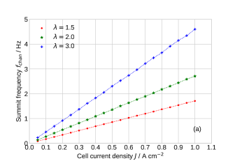
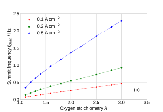
Figure 5: (a) The characteristic frequency of channel impedance $f_{chan}$ vs cell current density for the indicated air flow stoichiometries. (b) The frequency $f_{chan}$ vs air flow stoichiometry for the indicated cell current densities.

IV Conclusions

An analytical model for impedance of oxygen transport in the GDL and channel of a PEM fuel cell cathode is developed. The model is based on 1d+1d–coupled oxygen mass transport equations along the channel and through the GDL. The oxygen and proton transport through the cathode catalyst layer are assumed to be fast. Analytical solution for the GDL+channel impedance $Z_{gdlc}$ is obtained. The Nyquist spectrum of $Z_{gdlc}$ consists of two arcs, of which the left arcs corresponds to oxygen transport in the GDL and the right (LF) arc is due to oxygen transport in the channel. The characteristic frequency of the channel arc depends linearly on the oxygen stoichiometry. The shape of the GDL arc differs from the Warburg finite–length impedance due to effect of double layer charging in the catalyst layer attached to the GDL. For typical PEMFC parameters, the characteristic frequency of the GDL arc $f_{gdl}$ is close to the Warburg finite–length frequency. However, for larger CCL thickness the non–Warburg factor strongly shifts $f_{gdl}$ to lower values. At low catalyst layer thickness, the high–frequency feature in the spectrum of imaginary part of the GDL impedance forms. This effect is particularly important for identification of DRT peaks in low–Pt cell spectra, as low–Pt cells typically differ from the high–Pt cells by the catalyst layer thickness only.

Appendix A Equations for the factors $N_{c}$ and $D_{c}$ in Eq.(46)

$$N_{c}=\lambda^{2}\tilde{J}\left({{\rm e}^{2\tilde{\eta}_{0}}}+\left(\tilde{J}+{\rm i}\tilde{\omega}(1+\xi^{2})\right){{\rm e}^{\tilde{\eta}_{0}}}-\xi^{2}\tilde{\omega}^{2}\right)\\ \times\exp\left(\dfrac{-{{\rm e}^{\tilde{\eta}_{0}}}-{\rm i}\tilde{\omega}\xi^{2}}{\lambda\tilde{J}}\right)+\lambda\left({{\rm e}^{\tilde{\eta}_{0}}}-\lambda\tilde{J}+{\rm i}\tilde{\omega}\xi^{2}\right)\\ \times\left({{\rm e}^{2\tilde{\eta}_{0}}}+\left(\tilde{J}+{\rm i}\tilde{\omega}(\xi^{2}+1)\right){{\rm e}^{\tilde{\eta}_{0}}}-\xi^{2}\tilde{\omega}^{2}\right)\\ -\left({{\rm e}^{\tilde{\eta}_{0}}}+{\rm i}\tilde{\omega}\xi^{2}\right)^{2}{{\rm e}^{\tilde{\eta}_{0}}}/2$$ (48)

$$D_{c}=2\lambda^{2}\tilde{J}\left({{\rm e}^{2\tilde{\eta}_{0}}}+\left(\tilde{J}+{\rm i}\tilde{\omega}(1+\xi^{2})\right){{\rm e}^{\tilde{\eta}_{0}}}-\xi^{2}\tilde{\omega}^{2}\right)\\ \times\exp\left(\dfrac{-{{\rm e}^{\tilde{\eta}_{0}}}-{\rm i}\tilde{\omega}\xi^{2}}{\lambda\tilde{J}}\right){{\rm e}^{\tilde{\eta}_{0}}}\\ -2\lambda\xi^{6}\tilde{\omega}^{4}+{\rm i}\left(2\lambda\xi^{2}-\xi^{2}+4\lambda\right)\xi^{4}{{\rm e}^{\tilde{\eta}_{0}}}\,\tilde{\omega}^{3}\\ +2\xi^{2}\left(\left(2\lambda\xi^{2}-\xi^{2}+\lambda\right){{\rm e}^{\tilde{\eta}_{0}}}+\lambda^{2}\tilde{J}\right){{\rm e}^{\tilde{\eta}_{0}}}\tilde{\omega}^{2}\\ -{\rm i}\left(\left(2\lambda-1\right)\xi^{2}{{\rm e}^{\tilde{\eta}_{0}}}+2\lambda\tilde{J}\left(\lambda\xi^{2}-\xi^{2}+\lambda\right)\right){{\rm e}^{2\tilde{\eta}_{0}}}\tilde{\omega}\\ -2\lambda\tilde{J}\left(\left(\lambda-1\right){{\rm e}^{\tilde{\eta}_{0}}}+\lambda\tilde{J}\right){{\rm e}^{2\tilde{\eta}_{0}}}$$ (49)

Nomenclature

$\tilde{}$	Marks dimensionless variables
$b$	ORR Tafel slope, V
$C_{dl}$	Double layer volumetric capacitance, F cm-3
$c_{1}$	Oxygen molar concentration
	at the CCL/GDL interface, mol cm-3
$c_{b}$	Oxygen molar concentration in the GDL, mol cm-3
$c_{h}$	Oxygen molar concentration in the channel, mol cm-3
$c_{h}^{in}$	Reference (inlet) oxygen concentration, mol cm-3
$D_{b}$	Oxygen diffusion coefficient in the GDL, cm2 s-1
$F$	Faraday constant, C mol-1
$f$	Characteristic frequency, Hz
$i_{*}$	ORR volumetric exchange current density, A cm-3
${\rm i}$	Imaginary unit
$j$	Local proton current density along the CCL, A cm-2
$j_{\lim}$	Limiting current density
	due to oxygen transport in the GDL, Eq.(12) A cm-2
$j_{0}$	Local cell current density, A cm-2
$l_{b}$	GDL thickness, cm
$l_{t}$	CCL thickness, cm
$t$	Time, s
$t_{*}$	Characteristic time, s, Eq.(4)
$x$	Coordinate through the cell, cm
$Z$	Local impedance, Ohm cm2
$Z_{gdlc}$	GDL+channel impedance, Ohm cm2
$Z_{tot}$	Total cathode side impedance, including
	faradaic one, Ohm cm2
$z$	Coordinate along the cathode channel, cm

Subscripts:

$0$	Membrane/CCL interface
$1$	CCL/GDL interface
$b$	In the GDL
$gdl$	GDL
$gdlc$	GDL+channel
$f$	faradaic
$h$	Air channel
$W$	Warburg

Superscripts:

$0$	Steady–state value
$1$	Small–amplitude perturbation

Greek:

$\eta$	ORR overpotential, positive by convention, V
$\lambda$	Air flow stoichiometry, Eq.(28)
$\mu$	Dimensionless parameter, Eq.(20)
$\xi$	Dimensionless parameter, Eq.(28)
$\phi$	Dimensionless parameter. Eq.(24)
$\psi$	Dimensionless parameter. Eq.(24)
$\omega$	Angular frequency of the AC signal, s-1

References

- Lasia [2014] A. Lasia. Electrochemical Impedance Spectroscopy and its Applications. Springer, New York, 2014.
- Tang et al. [2020] Zh. Tang, Q.-A. Huang, Y.-J. Wang, F. Zhang, W. Li, A. Li, L. Zhang, and JJ Zhang. Recent progress in the use of electrochemical impedance spectroscopy for the measurement, monitoring, diagnosis and optimization of proton exchange membrane fuel cell performance. J. Power Sources, 468:228361, 2020. doi: 10.1016/j.jpowsour.2020.228361.
- Macdonald [2006] D. Macdonald. Reflections on the history of electrochemical impedance spectroscopy. Electrochim. Acta, 51:1376–1388, 2006. doi: 10.1016/j.electacta.2005.02.107.
- Huang et al. [2020] J. Huang, Y. Gao, J. Luo, S. Wang, C. Li, S. Chen, and J. Zhang. Editors’ choice–review–impedance response of porous electrodes: Theoretical framework, physical models and applications. J. Electrochem. Soc., 167:166503, 2020. doi: 10.1149/1945-7111/abc655.
- Fuoss and Kirkwood [1941] R.M. Fuoss and J.G. Kirkwood. Electrical properties of solids. viii. Dipole moments in polyvinyl chloride-diphenyl systems. J. Am. Chem. Soc., 63:385–394, 1941. doi: 10.1021/ja01847a013.
- Schichlein et al. [2002] H. Schichlein, A. C. Müller, M. Voigts, A. Krügel, and E. Ivers-Tiffée. Deconvolution of electrochemical impedance spectra for the identification of electrode reaction mechanisms in solid oxide fuel cells. J. Appl. Electrochem., 32:875–882, 2002. doi: 10.1023/A:1020599525160.
- Effendy et al. [2020] S. Effendy, J. Song, and M. Z. Bazant. Analysis, design, and generalization of electrochemical impedance spectroscopy (EIS) inversion algorithms. J. Electrochem. Soc., 167:106508, 2020. doi: 10.1149/1945-7111/ab9c82.
- Schneider et al. [2007a] I. A. Schneider, S. A. Freunberger, D. Kramer, A. Wokaun, and G. G. Scherer. Oscillations in gas channels. Part I. The forgotten player in impedance spectroscopy in PEFCs. J. Electrochem. Soc., 154:B383–B388, 2007a. doi: 10.1149/1.2435706.
- Schneider et al. [2007b] I. A. Schneider, D. Kramer, A. Wokaun, and G. G. Scherer. Oscillations in gas channels. II. Unraveling the characteristics of the low–frequency loop in air–fed PEFC impedance spectra. J. Electrochem. Soc., 154:B770–B3782, 2007b. doi: 10.1149/1.2742291.
- Kulikovsky [2012] A. A. Kulikovsky. A model for local impedance of the cathode side of PEM fuel cell with segmented electrodes. J. Electrochem. Soc., 159:F294–F300, 2012. doi: 10.1149/2.066207jes.
- Kulikovsky and Shamardina [2015] A. Kulikovsky and O. Shamardina. A model for PEM fuel cell impedance: Oxygen flow in the channel triggers spatial and frequency oscillations of the local impedance. J. Electrochem. Soc., 162:F1068–F1077, 2015. doi: 10.1149/2.0911509jes.
- Maranzana et al. [2012] G. Maranzana, J. Mainka, O. Lottin, J. Dillet, A. Lamibrac, A. Thomas, and S. Didierjean. A proton exchange membrane fuel cell impedance model taking into account convection along the air channel: On the bias between the low frequency limit of the impedance and the slope of the polarization curve. Electrochim. Acta, 83:13–27, 2012.
- Chevalier et al. [2016] S. Chevalier, C. Josset, A. Bazylak, and B. Auvity. Measurements of air velocities in polymer electrolyte membrane fuel cell channels using electrochemical impedance spectroscopy. J. Electrochem. Soc., 163:F816–F823, 2016. doi: 10.1149/2.0481608jes.
- Kulikovsky [2019] A. Kulikovsky. Analytical impedance of oxygen transport in a PEM fuel cell channel. J. Electrochem. Soc., 166:F306–F311, 2019. doi: 10.1149/2.0951904jes.
- Cruz-Manzo and Greenwood [2021] S. Cruz-Manzo and P. Greenwood. Analytical Warburg impedance model for EIS analysis of the gas diffusion layer with oxygen depletion in the air channel of a PEMFC. J. Electrochem. Soc., 168:074502, 2021. doi: 10.1149/1945-7111/ac1031.
- Reshetenko and Kulikovsky [2019] T. Reshetenko and A. Kulikovsky. On the distribution of local current density along the PEM fuel cell cathode channel. Electrochem. Comm., 101:35–38, 2019. doi: 10.1016/j.elecom.2019.02.005.
- Chevalier et al. [2018] S. Chevalier, C. Josset, and B. Auvity. Analytical solutions and dimensional analysis of pseudo 2D current density distribution model in PEM fuel cells. Renew. Energy, 125:738–746, 2018. doi: 10.1016/j.renene.2018.02.120.
- Kulikovsky [2003] A. A. Kulikovsky. The voltage current curve of a PEM fuel cell: Analytical and numerical modeling. In M. Laudon and B. Romanowicz, editors, Techn. Proc. of the 2003 Nanotechnology Conf. and Trade Show, volume 3, pages 467–470, San–Francisco, CA, USA, February 23–27 2003. Computational Publications.
- Kulikovsky [2004] A. A. Kulikovsky. The effect of stoichiometric ratio on the performance of a polymer electrolyte fuel cell. Electrochim. Acta, 49(4):617–625, 2004.
- Barbero [2016] G. Barbero. Warburg’s impedance revisited. Phys. Chem. Chem. Phys., 18:29537–29542, 2016. doi: 10.1039/c6cp05049b.
- Huang [2018] J. Huang. Diffusion impedance of electroactive materials, electrolytic solutions and porous electrodes: Warburg impedance and beyond. Electrochim. Acta, 281:170–188, 2018. doi: 10.1016/j.electacta.2018.05.136.
- Reshetenko et al. [2020] T. Reshetenko, G. Randolf, M. Odgaard, B. Zulevi, A. Serov, and A. Kulikovsky. The effect of proton conductivity of Fe-N-C–based cathode on PEM fuel cell performance. J. Electrochem. Soc., 167:084501, 2020. doi: 10.1149/1945-7111/ab8825.