A pressure-stabilized projection Lagrange–Galerkin scheme for the transient Oseen problem

Abstract

We propose and analyze a pressure-stabilized projection Lagrange–Galerkin scheme for the transient Oseen problem. The proposed scheme inherits the following advantages from the projection Lagrange–Galerkin scheme. The first advantage is computational efficiency. The scheme decouples the computation of each component of the velocity and pressure. The other advantage is essential unconditional stability. Here we also use the equal-order approximation for the velocity and pressure, and add a symmetric pressure stabilization term. This enriched pressure space enables us to obtain accurate solutions for small viscosity. First, we show an error estimate for the velocity for small viscosity. Then we show convergence results for the pressure. Numerical examples of a test problem show higher accuracy of the proposed scheme for small viscosity.

Keywords:

Transient Oseen problem, Lagrange–Galerkin method, fractional-step projection method, equal-order finite element, symmetric pressure stabilization, dependence on viscosity.

1 Introduction

We consider a finite element scheme for the transient Oseen problem, known as a linearization of the Navier–Stokes (NS) problem, with small viscosity. We need special cares to obtain accurate numerical solutions even in this linear problem.

We focus on the Lagrange–Galerkin (LG) method, which combines the method of the characteristics and Galerkin method. The LG method is a robust numerical technique for solving convection-dominated flow problems. It was first developed and analyzed in [18, 37], and the analysis for the NS problem was improved in [39]. The LG method is also applied to, e.g., natural convection problems [4] and viscoelastic models [32, 33]. One advantage of this method is the explicit treatment of the convection term so that the resulting matrix is symmetric. Moreover, the scheme is essentially unconditionally stable for the Oseen problem [35]. It means that stability conditions, such as $\Delta t\leq ch^{\alpha}$, are not needed, where $\Delta t$ is the time increment, $h$ is the mesh size, and $c$ and $\alpha$ are positive constants. We note that this stability is not influenced by small viscosity for the Oseen problem [35].

One of the main ingredients of this paper is the combination of LG and fractional-step projection methods. See [24] for the overview of the projection method. The main advantage is the computational efficiency that decouples the velocity and pressure. Achdou and Guermond [1] have proposed a combined scheme of the incremental pressure correction projection and LG method using the inf-sup stable elements for the NS problem. They have derived error estimates for the velocity and pressure when the viscosity constant is 1. They used the solution of a system of ordinary differential equations (ODEs) as the trajectory map, which should be approximated in practical computation. Misawa [34] has considered an Euler approximated scheme of [1] and error estimates of the same order have been derived for the velocity and pressure. However, in [25], instability of the scheme [1] has been observed for relatively large time increment and Reynolds number. There, they have implemented the scheme [1] with some approximation and have computed a flow behind a backward-facing step. Guermond and Minev [25] have developed an LG/projection scheme for the NS problem, which is stable under the same condition, and derived an error estimate for the velocity. The estimate for the pressure, however, is not known to the best of the author’s knowledge.

Here we also focus on the dependence on the inverse of the viscosity. The above estimates are of the forms $c(\Delta t^{\alpha}+h^{\beta})$. We note that the constant $c$ contains not only a Sobolev norm of the exact solution, $\|(u,p)\|_{X_{1}}$ but also a norm multiplied by the inverse of the viscosity, e.g., $\nu^{-1}\|(u,p)\|_{X_{2}}$. The effect of $\nu^{-1}$ in the latter term appears even when the exact solution does not show sharp boundary layers. See a recent survey [21].

One choice of eliminating the effect of the inverse of the viscosity is to enhance the divergence-free condition (mass conservation) by the grad-div stabilization [19]. Error analyses independent of the viscosity were performed for the Stokes problem [36], the transient Oseen problem [7, 12], and the transient NS problem [16] by relying on this term. However, a drawback is that the grad-div operator creates coupled matrices for the velocity [31].

Recently, without the grad-div stabilization, dependence on the inverse of the viscosity can be eliminated only by using equal-order pairs of finite elements with pressure stabilization, for the transient problems. Chen and Feng [9] have analyzed a semi-discrete scheme using the equal-order element with symmetric pressure stabilization for the transient NS problem to derive uniform error estimates with respect to the Reynolds number. De Frutos et al. [13] have analyzed a standard Galerkin scheme for the transient NS problem using the equal-order finite elements with local projection stabilization. Such estimates also hold for an LG scheme for the transient Oseen equations with the equal-order elements with the stabilization of Brezzi–Pitkäranta or its generalization to the higher order element [42].

In this paper, we propose a projection/LG scheme using the equal-order element with a pressure stabilization for the transient Oseen problem. The advantages of computational efficiency and essentially unconditional stability are inherited from the projection/LG scheme. The projection/LG part is based on Guermond and Minev for the inf-sup stable elements [25]. The pressure stabilized fractional-step projection part is mainly adopted from Burman et al. [7]. See also comments in Subsection 2.5 below. Firstly, we derive error estimates for the velocity in $L^{2}$-norm of order $\Delta t+h^{k}$ independent of the inverse of the viscosity, where $k$ is the degree of piecewise polynomials. Then, we show an error estimate of order $\Delta t+h^{k}$ for the pressure, which may depend on the viscosity. It is worth noting that even viscosity-dependent pressure estimates in the Oseen framework have not been obtained for the scheme [25] to the best of the author’s knowledge. The technical difficulty is, as in [12, 16, 22], the estimate of the time difference of the velocity.

We mention related works. Burman et al. [7] developed and analyzed a projection scheme for the Oseen problem. They used the equal-order elements with the continuous interior penalty method, and with terms including the grad-div and pressure stabilization. Robust error estimates with respect to the Reynolds numbers are derived for the velocity and a time-average of the pressure. The order is $\Delta t+h^{k+1/2}$ in $L^{2}$-norm for the velocity. The optimal estimate of order $\Delta t+h^{k+1}$ independent of the viscosity is not known so far [21]. De Frutos et al. [16, 17] proposed and analyzed a projection scheme for the NS problem. They used the inf-sup stable standard Galerkin method with the grad-div stabilization. They derived viscosity-independent error estimates for the velocity. It seems difficult to get the viscosity-independent estimate for the pressure with optimal order. García-Archilla et al. [22] analyzed the implicit Galerkin scheme with equal-order element and pressure stabilization for the NS problem and derived error estimates independent of the inverse of the viscosity. Badia and Codina [2] have developed and analyzed a non-incremental projection scheme for the NS problem using the equal-order element with a local projection type stabilization. De Frutos et al. [14, 15] have analyzed a projection scheme with non inf-sup stable elements for the Stokes and the NS problem. The stabilization term is the same as the discretized Laplacian in the pressure Poisson equation, thus, extra stabilization is not necessary. In these works [2, 14, 15], the condition $\Delta t\sim h^{2}$ is needed, and the error constant depends on the inverse of the viscosity.

The remainder of the paper is organized as follows. In the next section we state the Oseen problem and present a pressure-stabilized projection LG scheme with preparing notation. In Section 3 we show error estimates for the velocity with small viscosity and their proof. In Section 4 we show an error estimate for the pressure and its proof. In Section 5 we give some numerical results, where the Taylor–Hood pair and equal-order ones are compared. In Section 6 we give conclusions. In the appendix section we prove a lemma used in the LG methods.

2 Problem setting and a present scheme

2.1 Continuous problem

We prepare notation used throughout this paper, and state the Oseen problem.

Let $\Omega$ be a polygonal or polyhedral domain of $\mathbf{R}^{d}~{}(d=2,3)$. We use the Sobolev spaces $W^{m,p}(\Omega)$ equipped with the norm $\|\cdot\|_{m,p}$ and the seminorm $|\cdot|_{m,p}$ for $p\in[1,\infty]$ and a non-negative integer $m$. We denote $W^{0,p}(\Omega)$ by $L^{p}(\Omega)$. The space $W^{1,p}_{0}(\Omega)$ consists of functions in $W^{1,p}(\Omega)$ whose traces vanish on the boundary of $\Omega$. When $p=2$, we denote $W^{m,2}(\Omega)$ by $H^{m}(\Omega)$ and drop the subscript $2$ in the corresponding norm and seminorm. For the vector-valued function $w\in W^{1,\infty}(\Omega)^{d}$ we define the seminorm $|w|_{1,\infty}$ by

$$\biggl{\lVert}\biggl{[}\sum_{i,j=1}^{d}\left(\frac{\partial w_{i}}{\partial x_{j}}\right)^{2}\biggr{]}^{1/2}\biggr{\rVert}_{0,\infty}.$$

The pair of parentheses $(\cdot,\cdot)$ shows the $L^{2}(\Omega)^{i}$-inner product for $i=1,d$ or $d\times d$. The space $L^{2}_{0}(\Omega)$ consists of functions $q\in L^{2}(\Omega)$ satisfying $(q,1)=0$. The dual space of $H^{1}_{0}(\Omega)$ is denoted by $H^{-1}(\Omega)$ with the norm $\|\cdot\|_{-1}$. We also use the notation $|\cdot|_{m,K}$ and $(\cdot,\cdot)_{K}$ for the seminorm and the inner product on a set $K$, respectively.

Let $T>0$ be a time. For a Sobolev space $X(\Omega)^{i}$, $i=1,d$, we use the abbreviations $H^{m}(X)=H^{m}(0,T;X(\Omega)^{i})$ and $C(X)=C([0,T];X(\Omega)^{i})$. We define the function space $Z^{m}$ by

$$\begin{split}Z^{m}&:=\{v\in H^{j}(0,T;H^{m-j}(\Omega)^{d});~{}j=0,\dots,m,\|v\|_{Z^{m}}<\infty\},\\ \|v\|_{Z^{m}}&:=\biggl{(}\sum_{j=0}^{m}\|v\|_{H^{j}(0,T;H^{m-j}(\Omega)^{d})}^{2}\biggr{)}^{1/2}.\end{split}$$

We also use the notation $H^{m}(t_{1},t_{2};X)$ and $Z^{m}(t_{1},t_{2})$ for spaces on a time interval $(t_{1},t_{2})$.

We consider the Oseen problem: find $(u,p):\Omega\times(0,T)\to\mathbf{R}^{d}\times\mathbf{R}$ such that

$$\begin{split}\frac{\partial u}{\partial t}+(w\cdot\nabla)u-\nu\Delta u+\nabla p=f&\quad\text{in}\quad\Omega\times(0,T),\\ \nabla\cdot u=0&\quad\text{in}\quad\Omega\times(0,T),\\ u=0&\quad\text{on}\quad\partial\Omega\times(0,T),\\ u(\cdot,0)=u^{0}&\quad\text{in}\quad\Omega,\end{split}$$ (1)

where $\partial\Omega$ represents the boundary of $\Omega$, the constant $\nu(>0)$ represents a viscosity, and $w,f:\Omega\times(0,T)\to\mathbf{R}^{d}$ and $u^{0}:\Omega\to\mathbf{R}^{d}$ are given functions. We assume $w=0$ on $\partial\Omega$.

We define the bilinear forms $a$ on $H^{1}_{0}(\Omega)^{d}\times H^{1}_{0}(\Omega)^{d}$ by

$$a(u,v):=\nu(\nabla u,\nabla v).$$

Then, we can write the weak form of (1) as follows: find $(u,p):(0,T)\to H^{1}_{0}(\Omega)^{d}\times L^{2}_{0}(\Omega)$ such that for $t\in(0,T)$,

$$\left(\Bigl{(}\frac{\partial u}{\partial t}+(w\cdot\nabla)u\Bigr{)}(t),v\right)+a(u(t),v)+(\nabla p(t),v) =(f(t),v), ~{}\forall v\in H^{1}_{0}(\Omega)^{d},$$ (2a)

$$(\nabla\cdot u(t),q) =0,\quad \forall q\in L^{2}_{0}(\Omega),$$ (2b)

with $u(0)=u^{0}$.

2.2 Temporal discretization

Let $\Delta t>0$ be a time increment, $N_{T}:=\lfloor T/\Delta t\rfloor$ the number of time steps, $t^{n}:=n\Delta t$, and $\psi^{n}:=\psi(\cdot,t^{n})$ for a function $\psi$ defined in $\Omega\times(0,T)$.

Let $w$ be smooth. The characteristic curve $X(t;x,s)$ is defined by the solution of the system of the ODEs,

$$\begin{split}\frac{dX}{dt}(t;x,s)&=w(X(t;x,s),t),\quad t<s,\\ X(s;x,s)&=x.\end{split}$$ (3)

Then, we can write the material derivative term $\frac{\partial u}{\partial t}+(w\cdot\nabla)u$ as follows:

$$\left(\frac{\partial u}{\partial t}+(w\cdot\nabla)u\right)(X(t),t)=\frac{d}{dt}u(X(t),t).$$

For $w^{*}:\Omega\to\mathbf{R}^{d}$ we define the mapping $X_{1}(w^{*}):\Omega\to\mathbf{R}^{d}$ by

$$(X_{1}(w^{*}))(x):=x-w^{*}(x)\Delta t.$$ (4)

Remark 2.1.

The image of $x$ by $X_{1}(w(\cdot,t))$ is the approximate value of $X(t-\Delta t;x,t)$ obtained by solving (3) by the backward Euler method.

Then, it holds that

$$\frac{\partial u^{n}}{\partial t}+(w^{n}\cdot\nabla)u^{n}=\frac{u^{n}-u^{n-1}\circ X_{1}(w^{n-1})}{\Delta t}+O(\Delta t),$$

where the symbol $\circ$ stands for the composition of functions, e.g., $(g\circ f)(x):=g(f(x))$.

2.3 Spatial discretization

Let $\{\mathcal{T}_{h}\}_{h\downarrow 0}$ be a regular family of triangulations of $\overline{\Omega}$ [10], $h_{K}:=\operatorname{diam}(K)$ for an element $K\in\mathcal{T}_{h}$, and $h:=\max_{K\in\mathcal{T}_{h}}h_{K}$. For a positive integer $m$, the finite element space of order $m$ is defined by

$$W_{h}^{(m)}:=\{\psi_{h}\in C(\overline{\Omega});~{}\psi_{h|K}\in\mathrm{P}_{m}(K),~{}\forall K\in\mathcal{T}_{h}\},$$

where $\mathrm{P}_{m}(K)$ is the set of polynomials on $K$ whose degrees are equal to or less than $m$. For a pair of positive integers $(k,\ell)$, we define $\mathrm{P}_{k}/\mathrm{P}_{\ell}$-finite element space by

$$V_{h}\times Q_{h}:=[W_{h}^{(k)}\cap H_{0}^{1}(\Omega)]^{d}\times[W_{h}^{(\ell)}\cap L_{0}^{2}(\Omega)].$$

The space $Y_{h}:=V_{h}+\nabla Q_{h}$ is also used in the projection method [23]. We denote by $i_{h}^{T}$ the $L^{2}$-projector from $Y_{h}$ to $V_{h}$, which is the dual operator of $i_{h}$, the injection from $V_{h}$ to $Y_{h}$.

For the equal order $\mathrm{P}_{k}/\mathrm{P}_{k}$-element we use a symmetric positive semidefinite bilinear form $s_{1}:Q_{h}\times Q_{h}\to\mathbf{R}$ for stabilization, which is specified in Hypothesis 3 below. A typical example is

$$\begin{split}s_{1}(p_{h},q_{h}):=\sum_{K\in\mathcal{T}_{h}}h_{K}^{2k}\sum_{|\alpha|=k}(D^{\alpha}p_{h},D^{\alpha}q_{h})_{K},\end{split}$$ (5)

which is the stabilization by Brezzi and Pitkäranta [5] for the $\mathrm{P}_{1}/\mathrm{P}_{1}$-element and its extension to higher order elements [6]. We note that $s_{1}$ does not include the viscosity or a stabilization parameter. Practically a non-negative parameter $\delta$ is included in the stabilization term as follows:

$$s_{\delta}(p_{h},q_{h}):=\delta s_{1}(p_{h},q_{h}).$$

2.4 Present scheme

We are now in position to define our pressure-stabilized projection LG scheme called Scheme($k,\ell,\delta$). Let $\mathcal{T}_{h}$, $\Delta t$, integers $k,\ell\geq 1$ and a real number $\delta\geq 0$ be given.

Scheme($k,\ell,\delta$): Let $V_{h}\times Q_{h}$ be the $\mathrm{P}_{k}/\mathrm{P}_{\ell}$-finite element space on $\mathcal{T}_{h}$. Let $(u_{h}^{0},p_{h}^{0})\in Y_{h}\times Q_{h}$ be given. Find $(\widetilde{u}_{h}^{n},u_{h}^{n},p_{h}^{n})\in V_{h}\times Y_{h}\times Q_{h}$, $n=1,...,N_{T}$ such that for $n=0,1,...,N_{T}-1$

$$\biggl{(}\frac{\widetilde{u}_{h}^{n+1}-(i_{h}^{T}u_{h}^{n})\circ X_{1}(w^{n})}{\Delta t},v_{h}\biggr{)}+a(\widetilde{u}_{h}^{n+1},v_{h})+(\nabla p_{h}^{n},v_{h}) =(f^{n+1},v_{h}), \forall v_{h}\in V_{h},$$ (6a)

$$\frac{u_{h}^{n+1}-\widetilde{u}_{h}^{n+1}}{\Delta t}+\nabla(p_{h}^{n+1}-p_{h}^{n}) =0,$$ (6b)

$$(u_{h}^{n+1},\nabla q_{h})-s_{\delta}(p_{h}^{n+1},q_{h}) =0, \forall q_{h}\in Q_{h}.$$ (6c)

We later see in Lemma 3.4 that, for each $w^{n}\in W^{1,\infty}_{0}(\Omega)^{d}$ and under the condition $\Delta t|w^{n}|_{1,\infty}<1$, the inclusion $(X_{1}(w^{n}))(\Omega)\subset\Omega$ holds. Thus the composite function $(i_{h}^{T}u_{h}^{n})\circ X_{1}(w^{n})$ is well-defined on $\Omega$.

While we use $i_{h}^{T}u_{h}^{n}$ in the practical scheme, the variable $u_{h}^{n+1}$ is eliminated. For $n\geq 1$, we obtain the following practical scheme using the expression of $u_{h}^{n}$ in (6b), testing (6b) with $\nabla q_{h}$ and using (6c).

Stage 1: find $i_{h}^{T}u_{h}^{n}\in V_{h}$ such that

$$(i_{h}^{T}u_{h}^{n},v_{h})=(\widetilde{u}_{h}^{n}-\Delta t\nabla(p_{h}^{n}-p_{h}^{n-1}),v_{h}),\quad\forall v_{h}\in V_{h}.$$ (7)

Stage 2: find $\widetilde{u}_{h}^{n+1}\in V_{h}$ such that

$$\frac{1}{\Delta t}(\widetilde{u}_{h}^{n+1},v_{h})+a(\widetilde{u}_{h}^{n+1},v_{h})=\frac{1}{\Delta t}\left((i_{h}^{T}u_{h}^{n})\circ X_{1}(w^{n}),v_{h}\right)-\left(\nabla p_{h}^{n},v_{h}\right)+(f^{n+1},v_{h}),$$

$$\quad\forall v_{h}\in V_{h}.$$ (8)

Stage 3: find $p_{h}^{n+1}\in Q_{h}$ such that

$$(\nabla p_{h}^{n+1},\nabla q_{h})+\frac{1}{\Delta t}s_{\delta}(p_{h}^{n+1},q_{h})=(\nabla p_{h}^{n},\nabla q_{h})+\frac{1}{\Delta t}(\widetilde{u}_{h}^{n+1},\nabla q_{h}),\quad\forall q_{h}\in Q_{h}.$$ (9)

2.5 Comments on the scheme

This scheme has an advantage in computational cost. We can decouple the left-hand side of (7), and (8) into each velocity component, respectively, as follows:

$$(\widetilde{U}_{h1},v_{h1})+(\widetilde{U}_{h2},v_{h2}),$$

$$\Bigl{(}\frac{1}{\Delta t}(\widetilde{u}_{h1}^{n+1},v_{h1})+a(\widetilde{u}_{h1}^{n+1},v_{h1})\Bigr{)}+\Bigl{(}\frac{1}{\Delta t}(\widetilde{u}_{h2}^{n+1},v_{h2})+a(\widetilde{u}_{h2}^{n+1},v_{h2})\Bigr{)},$$

where $(\widetilde{U}_{h1},\widetilde{U}_{h2})=i_{h}^{T}u_{h}^{n}$, $(\widetilde{u}_{h1}^{n+1},\widetilde{u}_{h2}^{n+1})=\widetilde{u}_{h}^{n+1}$ and $(v_{h1},v_{h2})=v_{h}$ if $d=2$. Each part corresponds to the matrix in the discretized Poisson equation with the mass term, which is easy to handle by linear solvers such as the conjugate gradient method [3]. The matrix in (9) is the one in the discretized Poisson equation subject to the Neumann boundary condition with the symmetric stabilization term. In addition to the explicit treatment of the convection term, we do not need time restriction such as $\Delta t\leq ch^{\alpha}$ for the error estimates in this paper.

We adopt the framework of Guermond and Minev [25] for the combination of the projection and the LG methods. Achdou and Guermond [1] also developed the combined scheme for the NS equations. To show the corresponding formulation in [1], we replace (6a) by

$$\biggl{(}\frac{\widetilde{u}_{h}^{n+1}-u_{h}^{n}}{\Delta t},v_{h}\biggr{)}+\biggl{(}\frac{\widetilde{u}_{h}^{n}-\widetilde{u}_{h}^{n}\circ X_{1}(w^{n})}{\Delta t},v_{h}\biggr{)}+a(\widetilde{u}_{h}^{n+1},v_{h})+(\nabla p_{h}^{n},v_{h})=(f^{n+1},v_{h}).$$

Then (8) is replaced by the following form without $i_{h}^{T}u_{h}^{n}$:

$$\begin{split}\frac{1}{\Delta t}(\widetilde{u}_{h}^{n+1},v_{h})+a(\widetilde{u}_{h}^{n+1},v_{h})=\frac{1}{\Delta t}(\widetilde{u}_{h}^{n}\circ X_{1}(w^{n}),v_{h})-(\nabla(2p_{h}^{n}-p_{h}^{n-1}),v_{h})+(f^{n+1},v_{h}).\end{split}$$

However, it is difficult to derive the viscosity robust error estimate in Section 3.

Following Guermond and Minev [25], in (6a), we do not use the original $u_{h}^{n}\in Y_{h}$ but the $L^{2}$-projection $i_{h}^{T}u_{h}^{n}\in V_{h}$. Our error estimates in Sections 3 and 4 are also valid if we replace $i_{h}^{T}u_{h}^{n}$ by $u_{h}^{n}$. However, from the implementation viewpoint, we need to integrate the term $([\widetilde{u}_{h}^{n}-\nabla(p_{h}^{n}-p_{h}^{n-1})]\circ X_{1}(w^{n}),v_{h})$ in view of (6b).

In the scheme of Burman et al. [7], the pressure stabilization is defined a functional on $Y_{h}$. Here we simply define $s_{\delta}$ as the bilinear form on $Q_{h}$.

Finally, we mention an implementation issue. It is difficult to compute the term $((i_{h}^{T}u_{h}^{n})\circ X_{1}(w^{n}),v_{h})$ because the integrand is not polynomial on each element. It is known that rough numerical quadrature leads to instability. A remedy is to introduce a locally linearized velocity $w_{h}^{n}$, i.e., the $\mathrm{P}_{1}$-Lagrange interpolation of $w^{n}$ [41]. Then the term

$$((i_{h}^{T}u_{h}^{n})\circ X_{1}(w_{h}^{n}),v_{h})$$ (10)

can be exactly computable. The error estimates of this paper can be done with the Lagrange interpolation error of $O(h^{2})$ [40, 42].

3 Error estimates for the velocity with small viscosity

We use $c$ to represent a generic positive constant that is independent of $\nu$, $\Delta t$, $h$ and $\delta$ but depends on Sobolev norms of $w$, $u$ and $p$, and $T$, and may take a different value at each occurrence.

3.1 Hypotheses and the main theorem for the velocity

Hypothesis 1.

The velocity $w$ and the exact solution $(u,p)$ of the Oseen problem (1) satisfy

$$w\in C(W^{1,\infty}_{0})\cap H^{1}(L^{\infty}),\quad u\in Z^{2}\cap H^{1}(H^{k})\cap C(H^{k+1}),\quad p\in H^{1}(H^{1})\cap C(H^{k+1}).$$

Hypothesis 2.

The time increment $\Delta t$ satisfies $0<\Delta t\leq\Delta t_{0}$, where

$$\Delta t_{0}:=\frac{1}{4|w|_{C(W^{1,\infty})}}.$$

Hypothesis 3.

The bilinear form $s_{1}$ satisfies the following conditions.

1. $s_{1}:Q_{h}\times Q_{h}\to\mathbf{R}$ is a symmetric and positive semidefinite bilinear form.

2. For all $q_{h}\in Q_{h}$,

   $$s_{1}(q_{h},q_{h})\leq c\|q_{h}\|_{0}^{2}.$$

3. There exists an operator $\Pi_{h}:L^{2}_{0}(\Omega)\to Q_{h}$ such that

   $$\|q-\Pi_{h}q\|_{m} \leq ch^{s+1-m}\|q\|_{s+1},~{}q\in L^{2}_{0}(\Omega)\cap H^{s+1}(\Omega),~{}0\leq s\leq k,~{}m=0,1.$$ (11)

   $$s_{1}(\Pi_{h}q,\Pi_{h}q)^{1/2} \leq ch^{s}\|q\|_{s},~{}q\in L^{2}_{0}(\Omega)\cap H^{s}(\Omega),~{}0\leq s\leq k.$$ (12)

4. There is an operator $\mathcal{I}_{h}^{k}:V^{\mathrm{div}}\to V_{h}$ such that for all $v\in V^{\mathrm{div}}$ and $q_{h}\in Q_{h}$,

   $$|(\nabla\cdot(v-\mathcal{I}_{h}^{k}v),q_{h})| \leq c\biggl{(}\sum_{K\in\mathcal{T}_{h}}h_{K}^{-2}\|v-\mathcal{I}_{h}^{k}v\|_{0,K}^{2}+\|v-\mathcal{I}_{h}^{k}v\|_{1}^{2}\biggr{)}^{1/2}s_{1}(q_{h},q_{h})^{1/2},$$ (13)

   $$\|v-\mathcal{I}_{h}^{k}v\|_{m} \leq ch^{s+1-m}|v|_{s+1},~{}\forall v\in H^{s+1}(\Omega)^{d},~{}1\leq s\leq k,~{}m=0,1.$$ (14)

   Here, $V^{\mathrm{div}}=\{v\in H^{1}_{0}(\Omega)^{d};~{}\nabla\cdot v=0\}$.

In view Hypothesis 3-(1), we define the seminorm by

$$|q_{h}|_{s}=s_{1}(q_{h},q_{h})^{1/2},\quad\forall q_{h}\in Q_{h}.$$

Then, the Schwarz inequality holds:

$$s_{1}(q_{h},r_{h})\leq|q_{h}|_{s}|r_{h}|_{s},\quad\forall q_{h},r_{h}\in Q_{h}.$$

From (13) and (14) we easily get

$$|(\nabla\cdot(v-\mathcal{I}_{h}^{k}v),q_{h})|\leq ch^{k}|v|_{k+1}|q_{h}|_{s}\quad\forall v\in V^{\mathrm{div}}\cap H^{k+1}(\Omega)^{d},q_{h}\in Q_{h}.$$ (15)

The term $s_{1}$ in (5) and $\mathrm{P}_{k}/\mathrm{P}_{k}$-element ($k\geq 1$) space $V_{h}\times Q_{h}$ satisfy Hypothesis 3 with $\Pi_{h}$ being the Clément interpolation [11], and $\mathcal{I}_{h}^{k}$ being a modified Stokes projection [12] when $k\geq 2$, or Lagrange interpolation when $k=1$. See [22, 42]. We note that the constant does not depend on the viscosity.

Remark 3.1.

Hypothesis 3 is mainly adopted from [22] although (11) is slightly stronger. As pointed out there, these assumptions are quite similar to those in [8]. We refer to [22] for other stabilization satisfying Hypothesis 3.

Hypothesis 4.

The initial value $(u_{h}^{0},p_{h}^{0})$ is chosen so that there exists a positive constant $c$ independent of $h$ such that

$$\|u_{h}^{0}-u^{0}\|_{0}\leq ch^{k},\quad\|\nabla(p_{h}^{0}-p^{0})\|_{0}\leq c.$$

For a set of functions $\psi=\{\psi^{n}\}_{n=0}^{N_{T}}$ we use two norms $\|\cdot\|_{\ell^{\infty}(L^{2})}$ and $\|\cdot\|_{\ell^{2}(L^{2})}$ and a seminorm $|\cdot|_{\ell^{2}(s)}$ defined by

$$\begin{split}\|\psi\|_{\ell^{\infty}(L^{2})}&:=\max\left\{\|\psi^{n}\|_{0};n=0,\dots,N_{T}\right\},\\ \|\psi\|_{\ell^{2}(L^{2})}&:=\biggl{(}\Delta t\sum_{n=1}^{N_{T}}\|\psi^{n}\|_{0}^{2}\biggr{)}^{1/2},\quad|\psi|_{\ell^{2}(s)}:=\biggl{(}\Delta t\sum_{n=1}^{N_{T}}|\psi^{n}|_{s}^{2}\biggr{)}^{1/2}.\end{split}$$ (16)

Theorem 3.2.

Let $(u_{h},p_{h}):=\{(u_{h}^{n},p_{h}^{n})\}_{n=0}^{N_{T}}$ be the solution of Scheme$(k,k,\delta)$ with $k\geq 1$ and $\delta>0$. Assume Hypothesis 1, 2, 3, 4. Then the following estimate holds:

$$\begin{split}&\|u_{h}-u\|_{\ell^{\infty}(L^{2})},~{}\|\widetilde{u}_{h}-u\|_{\ell^{\infty}(L^{2})},~{}\nu^{1/2}\|\nabla(\widetilde{u}_{h}-u)\|_{\ell^{2}(L^{2})},~{}\delta^{1/2}|p_{h}-\Pi_{h}p|_{\ell^{2}(s)}\\ \leq&c(1+\nu^{1/2}+\delta^{1/2}+\delta^{-1/2})(\Delta t+h^{k}).\end{split}$$ (17)

Here, $\Pi_{h}p$ is the interpolation in Hypothesis 3.

3.2 Preliminaries for the velocity estimates

We use the techniques developed in the finite element projection method [23, 26], LG method [38, 40], combined method [1, 25], pressure-stabilized method [8, 20], and projection with pressure-stabilized method [7].

For a function $F$ defined on $[0,T]$, or sequence of functions $F=\{F^{n}\}_{n=0}^{N_{T}}$,

$$d_{t}F :=F-F(\cdot-\Delta t),\text{ or}$$

$$d_{t}F^{n} :=F^{n}-F^{n-1}.$$ (18)

Let $F\in H^{1}(X)$ or $H^{2}(X)$ for a Banach space $X(\Omega)^{i}$, $i=1,d$. The following inequalities are frequently used:

$$\|d_{t}F^{n}\|_{X} \leq\Delta t^{1/2}\Bigl{\|}\frac{\partial F}{\partial t}\Bigr{\|}_{L^{2}(t^{n-1},t^{n};X)},$$ (19)

$$\|d_{t}F^{n}-d_{t}F^{n-1}\|_{X} \leq c\Delta t^{3/2}\Bigl{\|}\frac{\partial^{2}F}{\partial t^{2}}\Bigr{\|}_{L^{2}(t^{n-2},t^{n};X)}.$$ (20)

First we recall a discrete version of the Gronwall inequality.

Lemma 3.3 (discrete Gronwall inequality).

Let $\gamma_{1}$ be a non-negative number, $\Delta t$ be a positive number, and $\{x^{n}\}_{n\geq n_{0}},\{y^{n}\}_{n\geq n_{0}+1}$ and $\{b^{n}\}_{n\geq n_{0}+1}$ be non-negative sequences. Suppose

$$\frac{x^{n}-x^{n-1}}{\Delta t}+y^{n}\leq\gamma_{1}x^{n-1}+b^{n},~{}\forall n\geq n_{0}+1.$$

Then, it holds that

$$x^{n}+\Delta t\sum_{i=n_{0}+1}^{n}y^{i}\leq\exp[\gamma_{1}(n-n_{0})\Delta t]\left(x^{n_{0}}+\Delta t\sum_{i=n_{0}+1}^{n}b^{i}\right),~{}\forall n\geq n_{0}+1.$$

Lemma 3.3 is shown by using the inequalities

$$\begin{split}x^{n}+y^{n}\Delta t&\leq(1+\gamma_{1}\Delta t)x^{n-1}+b^{n}\Delta t\leq\exp(\gamma_{1}\Delta t)(x^{n-1}+b^{n}\Delta t).\end{split}$$

Instead of the well-known summation form of the discrete Gronwall inequality, e.g., in [28], we use this form because the condition on $\Delta t$ does not include $\gamma_{1}$, making the proof simpler.

We prepare fundamental properties of the mapping $X_{1}(w^{*})$ for $w^{*}\in W^{1,\infty}_{0}(\Omega)^{d}$. We refer to [38, 40] for the proofs.

Lemma 3.4.

Let $w^{*}\in W^{1,\infty}_{0}(\Omega)^{d}$ and $X_{1}(w^{*})$ be the mapping defined in (4).

1. Under the condition $\Delta t|w^{*}|_{1,\infty}<1$, it holds that $(X_{1}(w^{*}))(\Omega)\subset\Omega$ and $X_{1}(w^{*}):\Omega\to\Omega$ is bijective.

2. Under the condition $\Delta t|w^{*}|_{1,\infty}\leq 1/4$, the estimate

   $$\frac{1}{2}\leq J\leq\frac{3}{2}$$

   holds, where $J$ is the Jacobian of $X_{1}(w^{*})$.

3. Under the condition $\Delta t|w^{*}|_{1,\infty}\leq 1/4$, there exists a positive constant $c$ independent of $\Delta t$ such that for $v\in L^{2}(\Omega)^{d}$

   $$\|v\circ X_{1}(w^{*})\|_{0}^{2}\leq(1+c|w^{*}|_{1,\infty}\Delta t)\|v\|_{0}^{2}.$$

Lemma 3.5 is fundamental to establishing the stability in the error equations for the projection methods. We give a proof for completeness although it is natural extension of the classical argument [23, 26], and is derived in a similar way to Lemma 4.1 in [7].

Lemma 3.5.

Let $\{\widetilde{U}_{h}^{n}\}_{n=n_{0}}^{n_{1}}\subset V_{h}$, $\{U_{h}^{n}\}_{n=n_{0}}^{n_{1}}\subset Y_{h}$, $\{G^{n}\}_{n=n_{0}}^{n_{1}}\subset L^{2}(\Omega)^{d}$, and $\{P_{h}^{n}\}_{n=n_{0}}^{n_{1}}$, $\{\Psi_{h}^{n}\}_{n=n_{0}}^{n_{1}}\subset Q_{h}$, satisfy for $n=n_{0},n_{0}+1,...,n_{1}-1$,

$$\biggl{(}\frac{\widetilde{U}_{h}^{n+1}-G^{n}}{\Delta t},v_{h}\biggr{)}+a(\widetilde{U}_{h}^{n+1},v_{h})+(\nabla\Psi_{h}^{n},v_{h}) =\langle F^{n+1},v_{h}\rangle,~{}\forall v_{h}\in V_{h},$$ (21a)

$$\frac{U_{h}^{n+1}-\widetilde{U}_{h}^{n+1}}{\Delta t}+\nabla(P_{h}^{n+1}-\Psi_{h}^{n}) =0,$$ (21b)

$$(U_{h}^{n+1},\nabla q_{h})-s_{\delta}(P_{h}^{n+1},q_{h}) =\langle S^{n+1},q_{h}\rangle,~{}\forall q_{h}\in Q_{h},$$ (21c)

with $F^{n+1}$ and $S^{n+1}$ being linear functionals on $V_{h}$ and $Q_{h}$, respectively. Then, it holds that for $n=n_{0},n_{0}+1,...,n_{1}-1$

$$\begin{split}&\frac{1}{2\Delta t}(\|U_{h}^{n+1}\|_{0}^{2}-\|G^{n}\|_{0}^{2}+\|\widetilde{U}_{h}^{n+1}-G^{n}\|_{0}^{2})\\ &+\nu\|\nabla\widetilde{U}_{h}^{n+1}\|_{0}^{2}+\frac{\Delta t}{2}(\|\nabla P_{h}^{n+1}\|_{0}^{2}-\|\nabla\Psi_{h}^{n}\|_{0}^{2})+\delta|P_{h}^{n+1}|_{s}^{2}\\ =&\langle F^{n+1},\widetilde{U}_{h}^{n+1}\rangle-\langle S^{n+1},P_{h}^{n+1}\rangle.\end{split}$$ (22)

Proof.

The equation (21a) with $v_{h}=\widetilde{U}_{h}^{n+1}$, and the identity $(a-b)a=\frac{1}{2}a^{2}-\frac{1}{2}b^{2}+\frac{1}{2}(a-b)^{2}$ yields

$$\begin{split}&\frac{1}{2\Delta t}(\|\widetilde{U}_{h}^{n+1}\|_{0}^{2}-\|G^{n}\|_{0}^{2}+\|\widetilde{U}_{h}^{n+1}-G^{n}\|_{0}^{2})\\ &+\nu\|\nabla\widetilde{U}_{h}^{n+1}\|_{0}^{2}+(\nabla\Psi_{h}^{n},\widetilde{U}_{h}^{n+1})=\langle F^{n+1},\widetilde{U}_{h}^{n+1}\rangle.\end{split}$$ (23)

Testing (21b) with $\Delta t\nabla\Psi_{h}^{n}$ and using the identity $(a-b)b=\frac{1}{2}a^{2}-\frac{1}{2}b^{2}-\frac{1}{2}(a-b)^{2}$, and again using (21b), we have

$$(U_{h}^{n+1}-\widetilde{U}_{h}^{n+1},\nabla\Psi_{h}^{n})+\frac{\Delta t}{2}(\|\nabla P_{h}^{n+1}\|_{0}^{2}-\|\nabla\Psi_{h}^{n}\|_{0}^{2})-\frac{1}{2\Delta t}\|U_{h}^{n+1}-\widetilde{U}_{h}^{n+1}\|_{0}^{2}=0.$$ (24)

Testing (21b) with $U_{h}^{n+1}$ yields

$$\begin{split}\frac{1}{2\Delta t}(\|U_{h}^{n+1}\|_{0}^{2}-\|\widetilde{U}_{h}^{n+1}\|_{0}^{2}&+\|U_{h}^{n+1}-\widetilde{U}_{h}^{n+1}\|_{0}^{2})\\ &+(\nabla P_{h}^{n+1},U_{h}^{n+1})-(\nabla\Psi_{h}^{n},U_{h}^{n+1})=0.\end{split}$$ (25)

Finally, (21c) with $q_{h}=P_{h}^{n+1}$ yields

$$(U_{h}^{n+1},\nabla P_{h}^{n+1})-\delta|P_{h}^{n+1}|_{s}^{2}=\langle S^{n+1},P_{h}^{n+1}\rangle.$$ (26)

Adding (23)–(25) and subtracting (26), we have the conclusion (22). ∎

Remark 3.6.

In Lemma 4.1 of [7], the corresponding estimate is not based on $U_{h}^{n}$ but on $i_{h}^{T}U_{h}^{n}$, and the stabilization term is functional on $Y_{h}$.

3.3 Proof of Theorem 3.2

Let $(z_{h}(t),r_{h}(t))\in V_{h}\times Q_{h}$ be the interpolation $(\mathcal{I}_{h}^{k}u(t),\Pi_{h}p(t))$ in Hypothesis 3. We use the following notation:

$$e_{h}^{n} =u_{h}^{n}-z_{h}^{n}, \widetilde{e}_{h}^{n} =\widetilde{u}_{h}^{n}-z_{h}^{n}, \eta(t) =u(t)-z_{h}(t),$$ (27a)

$$\varepsilon_{h}^{n} =p_{h}^{n}-r_{h}^{n}, \psi_{h}^{n} =p_{h}^{n}-r_{h}^{n+1}, X_{1}^{n} =X_{1}(w^{n}).$$ (27b)

We begin with error equations in $e_{h}^{n}$, $\widetilde{e}_{h}^{n}$ and $\varepsilon_{h}^{n}$. Connecting (6a) and (2a) at $t=t^{n+1}$, subtracting

$$\biggl{(}\frac{z_{h}^{n+1}-z_{h}^{n}\circ X_{1}^{n}}{\Delta t},v_{h}\biggr{)}+a(z_{h}^{n+1},v_{h})+(\nabla r_{h}^{n+1},v_{h}),$$

$$(z_{h}^{n+1},\nabla q_{h})-s_{\delta}(r_{h}^{n+1},q_{h})$$

from both sides of (6a) (equaling (2a)) and (6c), respectively, and noting $i_{h}^{T}z_{h}^{n}=z_{h}^{n}$, we get the following error equation for $n=0,1,...,N_{T}-1$.

$$\biggl{(}\frac{\widetilde{e}_{h}^{n+1}-(i_{h}^{T}e_{h}^{n})\circ X_{1}^{n}}{\Delta t},v_{h}\biggr{)}+a(\widetilde{e}_{h}^{n+1},v_{h})+(\nabla\psi_{h}^{n},v_{h}) =\bigl{\langle}R_{1}^{n+1},v_{h}\bigr{\rangle},~{} \forall v_{h}\in V_{h},$$ (28a)

$$\frac{e_{h}^{n+1}-\widetilde{e}_{h}^{n+1}}{\Delta t}+\nabla(\varepsilon_{h}^{n+1}-\psi_{h}^{n}) =0,$$ (28b)

$$(e_{h}^{n+1},\nabla q_{h})-s_{\delta}(\varepsilon_{h}^{n+1},q_{h}) =\langle S_{1}^{n+1},q_{h}\rangle,~{} \forall q_{h}\in Q_{h},$$ (28c)

where

$$\bigl{\langle}R_{1}^{n+1},v_{h}\bigr{\rangle} :=(R_{11}^{n+1}+R_{12}^{n+1},v_{h})+a(\eta^{n+1},v_{h})+(\nabla(p^{n+1}-r_{h}^{n+1}),v_{h}),$$

$$R_{11}^{n+1} :=\frac{\partial u^{n+1}}{\partial t}+(w^{n+1}\cdot\nabla)u^{n+1}-\frac{u^{n+1}-u^{n}\circ X_{1}^{n}}{\Delta t},$$ (29)

$$R_{12}^{n+1} :=\frac{\eta^{n+1}-\eta^{n}\circ X_{1}^{n}}{\Delta t},$$ (30)

$$\bigl{\langle}S_{1}^{n+1},q_{h}\bigr{\rangle} :=-(z_{h}^{n+1},\nabla q_{h})+s_{\delta}(r_{h}^{n+1},q_{h}).$$

Since the estimates of $R_{11}^{n}$ and $R_{12}^{n}$ are obtained by standard techniques used in the LG method (e.g. Lemmas 8, 10 in [42]), we omit their proofs.

Lemma 3.7.

Suppose that $w\in C(W^{1,\infty}_{0})\cap H^{1}(L^{\infty})$ and $\Delta t|w|_{C(W^{1,\infty})}\leq 1/4$. Then, there exists a positive constant $c$ depending on the norm $\|w\|_{C(L^{\infty})}$ such that

$$\|R_{11}^{n}\|_{0}\leq c\sqrt{\Delta t}\biggl{(}\|u\|_{Z^{2}(t^{n-1},t^{n})}+\left\|\frac{\partial w}{\partial t}\right\|_{L^{2}(t^{n-1},t^{n};L^{\infty})}\|\nabla u^{n}\|_{0}\biggr{)},\quad\forall u\in Z^{2},$$

$$\left\|\frac{v^{n}-v^{n-1}\circ X_{1}^{n-1}}{\Delta t}\right\|_{0}\leq\frac{c}{\sqrt{\Delta t}}\left\|v\right\|_{H^{1}(t^{n-1},t^{n};L^{2})\cap L^{2}(t^{n-1},t^{n};H^{1})},\quad\forall v\in H^{1}(L^{2})\cap L^{2}(H^{1}).$$

Proof of Theorem 3.2.

We apply Lemma 3.5 to (28) and obtain

$$\frac{1}{2\Delta t}(\|e_{h}^{n+1}\|_{0}^{2}-\|(i_{h}^{T}e_{h}^{n})\circ X_{1}^{n}\|_{0}^{2}+\|\widetilde{e}_{h}^{n+1}-(i_{h}^{T}e_{h}^{n})\circ X_{1}^{n}\|_{0}^{2})+\nu\|\nabla\widetilde{e}_{h}^{n+1}\|_{0}^{2}$$

$$+\delta|\varepsilon_{h}^{n+1}|_{s}^{2}+\frac{\Delta t}{2}(\|\nabla\varepsilon_{h}^{n+1}\|_{0}^{2}-\|\nabla\psi_{h}^{n}\|_{0}^{2})=\langle R_{1}^{n+1},\widetilde{e}_{h}^{n+1}\rangle-\langle S_{1}^{n+1},\varepsilon_{h}^{n+1}\rangle.$$ (31)

For the estimate of $\|\widetilde{e}_{h}^{n+1}\|_{0}$ we fix a $\gamma_{0}$ such that $\Delta t_{0}\leq\frac{1}{8\gamma_{0}}$. In the following we will get the bounds for $|\langle R_{1}^{n+1},\widetilde{e}_{h}^{n+1}\rangle|$ and $|\langle S_{1}^{n+1},\varepsilon_{h}^{n+1}\rangle|$ in the same way as in [42]. From the Schwarz’s inequality,

$$|(R^{n+1}_{1i},\widetilde{e}_{h}^{n+1})|\leq\frac{1}{\gamma_{0}}\|R_{1i}^{n+1}\|_{0}^{2}+\frac{\gamma_{0}}{4}\|\widetilde{e}_{h}^{n+1}\|_{0}^{2},~{}i=1,2.$$ (32)

Estimates for $\|R_{1i}^{n+1}\|_{0}^{2}$, $i=1,2$, are obtained by Lemma 3.7 with $v=\eta$, and the following estimate is obtained by (14):

$$\|\eta\|_{H^{1}(t^{n},t^{n+1};L^{2})\cap L^{2}(t^{n},t^{n+1};H^{1})}\leq ch^{k}\|u\|_{H^{1}(t^{n},t^{n+1};H^{k})\cap L^{2}(t^{n},t^{n+1};H^{k+1})}.$$

Bounds for the other terms in $\langle R_{1}^{n+1},\widetilde{e}_{h}^{n+1}\rangle$ are easily obtained from (14) and (11):

$$|a(\eta^{n+1},\widetilde{e}_{h}^{n+1})|\leq\frac{\nu}{2}\|\nabla\eta^{n+1}\|_{0}^{2} +\frac{\nu}{2}\|\nabla\widetilde{e}_{h}^{n+1}\|_{0}^{2}\leq c\nu h^{2k}\|u^{n+1}\|_{k+1}^{2}+\frac{\nu}{2}\|\nabla\widetilde{e}_{h}^{n+1}\|_{0}^{2},$$

$$|(\nabla(p^{n+1}-r_{h}^{n+1}),\widetilde{e}_{h}^{n+1})| \leq\frac{1}{\gamma_{0}}\|\nabla(p^{n+1}-r_{h}^{n+1})\|_{0}^{2}+\frac{\gamma_{0}}{4}\|\widetilde{e}_{h}^{n+1}\|_{0}^{2}$$

$$\leq ch^{2k}\|p^{n+1}\|_{k+1}^{2}+\frac{\gamma_{0}}{4}\|\widetilde{e}_{h}^{n+1}\|_{0}^{2}.$$ (33)

Bounds for the terms in $\langle S_{1}^{n+1},\varepsilon_{h}^{n+1}\rangle$ are obtained from (15) and (12) as follows:

$$|(z_{h}^{n+1},\nabla\varepsilon_{h}^{n+1})| =|(\nabla\cdot(z_{h}^{n+1}-u^{n+1}),\varepsilon_{h}^{n+1})|\leq ch^{k}\|u^{n+1}\|_{k+1}|\varepsilon_{h}^{n+1}|_{s}$$

$$\leq\frac{c}{\delta}h^{2k}\|u^{n+1}\|_{k+1}^{2}+\frac{\delta}{4}|\varepsilon_{h}^{n+1}|_{s}^{2}.$$

$$|s_{\delta}(r_{h}^{n+1},\varepsilon_{h}^{n+1})| \leq\delta|r_{h}^{n+1}|_{s}|\varepsilon_{h}^{n+1}|_{s}$$

$$\leq\delta|r_{h}^{n+1}|_{s}^{2}+\frac{\delta}{4}|\varepsilon_{h}^{n+1}|_{s}^{2}\leq c\delta h^{2k}\|p^{n+1}\|_{k}^{2}+\frac{\delta}{4}|\varepsilon_{h}^{n+1}|_{s}^{2}.$$

For $\|\widetilde{e}_{h}^{n+1}\|_{0}^{2}$ in (32) and (33)

$$\gamma_{0}\|\widetilde{e}_{h}^{n+1}\|_{0}^{2}\leq 2\gamma_{0}\|\widetilde{e}_{h}^{n+1}-(i_{h}^{T}e_{h}^{n})\circ X_{1}^{n}\|_{0}^{2}+2\gamma_{0}\|(i_{h}^{T}e_{h}^{n})\circ X_{1}^{n}\|_{0}^{2},$$ (34)

and since $2\gamma_{0}\leq\frac{1}{4\Delta t_{0}}<\frac{1}{2\Delta t}$, the first term is absorbed by the left hand side of (31). From Lemma 3.4 and since $i_{h}^{T}$ is the $L^{2}$-projector,

$$\|(i_{h}^{T}e_{h}^{n})\circ X_{1}^{n}\|_{0}^{2}\leq(1+c\Delta t)\|i_{h}^{T}e_{h}^{n}\|_{0}^{2}\leq(1+c\Delta t)\|e_{h}^{n}\|_{0}^{2}.$$ (35)

The estimate for $\|\nabla\psi_{h}^{n}\|_{0}^{2}$ is obtained by (19) as follows:

$$\begin{split}\|\nabla\psi_{h}^{n}\|_{0}^{2}&=\|\nabla\varepsilon_{h}^{n}-\nabla(r_{h}^{n+1}-r_{h}^{n})\|_{0}^{2}\\ &\leq(1+\Delta t)\|\nabla\varepsilon_{h}^{n}\|_{0}^{2}+\Bigl{(}1+\frac{1}{\Delta t}\Bigr{)}\|\nabla(r_{h}^{n+1}-r_{h}^{n})\|_{0}^{2},\\ &\leq(1+\Delta t)\|\nabla\varepsilon_{h}^{n}\|_{0}^{2}+c\|r_{h}\|_{H^{1}(t^{n},t^{n+1};H^{1})}^{2}.\end{split}$$ (36)

We note that $\|r_{h}\|_{H^{1}(t^{n},t^{n+1};H^{1})}\leq c\|p\|_{H^{1}(t^{n},t^{n+1};H^{1})}$ by (11).

Combining these estimates, from (31), we now obtain for $n=0,1,...,N_{T}-1$,

$$\frac{x^{n+1}-x^{n}}{\Delta t}+y^{n+1}\leq cx^{n}+cb^{n+1},$$ (37)

where

$$x^{n}= \|e_{h}^{n}\|_{0}^{2}+\Delta t^{2}\|\nabla\varepsilon_{h}^{n}\|_{0}^{2},$$

$$y^{n}= \frac{1}{2\Delta t}\|\widetilde{e}_{h}^{n}-(i_{h}^{T}e_{h}^{n-1})\circ X_{1}^{n-1}\|_{0}^{2}+\nu\|\nabla\widetilde{e}_{h}^{n}\|_{0}^{2}+\delta|\varepsilon_{h}^{n}|_{s}^{2},$$

$$b^{n}= \Delta t(\|u\|_{Z^{2}(t^{n-1},t^{n})}^{2}+\|w\|_{H^{1}(t^{n-1},t^{n};L^{\infty})}^{2}+\|p\|_{H^{1}(t^{n-1},t^{n};H^{1})}^{2})$$

$$+\frac{ch^{2k}}{\Delta t}\|u\|_{H^{1}(t^{n-1},t^{n};H^{k})\cap L^{2}(t^{n-1},t^{n};H^{k+1})}^{2}+c(1+\nu+\delta+\delta^{-1})h^{2k},$$

and $c$ is a constant depending on the Sobolev norms of $u$, $p$ and $w$, the constants in Hypothesis 3 and in Lemmas 3.4 and 3.7. We apply Lemma 3.3 to (37) and obtain

$$\begin{split}&\|e_{h}^{n}\|_{0}^{2}+\Delta t\sum_{i=1}^{n}\nu\|\widetilde{e}_{h}^{i}\|_{0}^{2}+\frac{1}{2}\sum_{i=1}^{n}\|\widetilde{e}_{h}^{i}-(i_{h}^{T}e_{h}^{i-1})\circ X_{1}^{i-1}\|_{0}^{2}+\Delta t\sum_{i=1}^{n}\delta|\varepsilon_{h}^{i}|_{s}^{2}\\ \leq&c(1+\nu+\delta+\delta^{-1})(\|e_{h}^{0}\|_{0}^{2}+\Delta t^{2}\|\nabla\varepsilon_{h}^{0}\|_{0}^{2}+\Delta t^{2}+h^{2k}).\end{split}$$ (38)

The estimate for the initial values are easily obtained from Hypotheses 4 and 3:

$$\|e_{h}^{0}\|_{0} \leq\|u_{h}^{0}-u^{0}\|_{0}+\|u^{0}-z_{h}^{0}\|_{0}\leq ch^{k},$$

$$\Delta t\|\nabla\varepsilon_{h}^{0}\|_{0} \leq\Delta t\|\nabla(p_{h}^{0}-p^{0})\|_{0}+\Delta t\|\nabla(p^{0}-r_{h}^{0})\|_{0}\leq c\Delta t.$$

Now, the conclusion (17) follows from the triangle inequalities applied to $u_{h}-u=e_{h}-\eta$ and $\widetilde{u}_{h}-u=\widetilde{e}_{h}-\eta$, (38), and (14) for $\eta$. We note that the estimate of $\|\widetilde{e}_{h}^{n}\|_{0}$ follows from (34), (35) and (38). ∎

4 An error estimate for the pressure

In this section, to concentrate on the convergence order, we also use the notation $c_{\nu,\delta}$ that may depend on $\nu,1/\nu,\delta$ and $1/\delta$. Additionally, we use notation and Lemmas in Subsections 3.1 and 3.2.

4.1 Hypotheses and the main theorem for the pressure

Hypothesis 5.

The velocity $w$ and the exact solution $(u,p)$ of the Oseen problem (1) satisfy

$$w\in W^{2,\infty}(L^{\infty})\cap H^{1}(W^{1,\infty}_{0}),\quad u\in Z^{3}\cap H^{2}(H^{k+1}),\quad p\in H^{2}(H^{k}).$$

We introduce the Stokes projection $(\widehat{u}_{h}^{*},\widehat{p}_{h}^{*})\in V_{h}\times Q_{h}$ of $(u^{*},p^{*})\in H^{1}_{0}(\Omega)^{d}\times L^{2}_{0}(\Omega)$, which satisfies the following equations:

$$a(\widehat{u}_{h}^{*},v_{h})-(\widehat{p}_{h}^{*},\nabla\cdot v_{h}) =a(u^{*},v_{h})-(p^{*},\nabla\cdot v_{h})\quad \forall v_{h}\in V_{h},$$ (39a)

$$-(\nabla\cdot\widehat{u}_{h}^{*},q_{h})-s_{\delta}(\widehat{p}_{h}^{*},q_{h}) =-(\nabla\cdot u^{*},q_{h}) \forall q_{h}\in Q_{h}.$$ (39b)

Hypothesis 6.

The initial value $(u_{h}^{0},p_{h}^{0})$ satisfies $(u_{h}^{0},p_{h}^{0})=(\widehat{u}_{h}^{0},\widehat{p}_{h}^{0})$.

Theorem 4.1.

Let $(u_{h},p_{h}):=\{(u_{h}^{n},p_{h}^{n})\}_{n=0}^{N_{T}}$ be the solution of Scheme$(k,k,\delta)$ with $k\geq 1$ and $\delta>0$. Hypotheses 5, 2, 3, and 6. Then the following estimate holds:

$$\|p_{h}-p\|_{\ell^{2}(L^{2})}\leq c_{\nu,\delta}(\Delta t+h^{k}).$$ (40)

Remark 4.2.

For the initial value,

$$\|u_{h}^{0}-\widehat{u}_{h}^{0}\|_{0},~{}\Delta t\|\nabla(p_{h}^{0}-\widehat{p}_{h}^{0})\|_{0}\leq c_{\nu,\delta}\Delta t(\Delta t+h^{k})$$

is actually needed in the proof of Theorem 4.1 as in [1, 26]. Hypothesis 6 is a sufficient condition.

4.2 Preliminaries for the pressure estimate

Lemma 4.3 is the weak inf-sup condition proved in [8].

Lemma 4.3.

Under Hypothesis 3, there exists a positive constant $c$ independent of $h$ such that

$$\|q_{h}\|_{0}\leq c\sup_{v_{h}\in V_{h}\setminus\{0\}}\frac{(\nabla\cdot v_{h},q_{h})}{\|v_{h}\|_{1}}+cs_{1}(q_{h},q_{h})^{1/2},~{}\forall q_{h}\in Q_{h}.$$

Lemma 4.4 is the error estimate of the Stokes projection in (39). We omit the proof since it is the standard argument (e.g. [20, 22]). We note that the constant $c_{\nu,\delta}$ may depend on $\nu$ and $\delta$.

Lemma 4.4.

Let $V_{h}\times Q_{h}$ be the $\mathrm{P}_{k}/\mathrm{P}_{k}$-element for $k\geq 1$. Suppose $(u^{*},p^{*})\in[H^{k+1}(\Omega)^{d}\cap H^{1}_{0}(\Omega)^{d}]\times[H^{k}(\Omega)\cap L^{2}_{0}(\Omega)]$. Assume Hypothesis 3 and $\delta>0$. Then, there exists a positive constant $c_{\nu,\delta}$ independent of $h$ such that for any $h$ the Stokes projection $(\widehat{u}_{h}^{*},\widehat{p}_{h}^{*})$ of $(u^{*},p^{*})$ defined in (39) satisfies

$$\|\nabla(u^{*}-\widehat{u}_{h}^{*})\|_{0},~{}\|p^{*}-\widehat{p}_{h}^{*}\|_{0}\leq c_{\nu,\delta}h^{\ell}(\|u^{*}\|_{\ell+1}+\|p^{*}\|_{\ell}),\quad 1\leq\ell\leq k.$$ (41)

Lemma 4.5 is a direct consequence of Lemma 4.5 in [1], and Lemma 3.4-(2) in this paper.

Lemma 4.5.

Let $1\leq q<\infty$, $1\leq p\leq\infty$, $1/p+1/p^{\prime}=1$ and $w_{i}\in W_{0}^{1,\infty}(\Omega)^{d}$, $i=1,2$. Under the condition $\Delta t|w_{i}|_{1,\infty}\leq 1/4$, it holds that, for $v\in W^{1,qp^{\prime}}(\Omega)^{d}$,

$$\|v\circ X_{1}(w_{1})-v\circ X_{1}(w_{2})\|_{0,q}\leq 2^{1/(qp^{\prime})}\Delta t\|w_{1}-w_{2}\|_{0,pq}\|\nabla v\|_{0,qp^{\prime}},$$

where $X_{1}(\cdot)$ is defined in (4).

Lemma 4.6.

Let $w_{i}\in W^{1,\infty}_{0}(\Omega)^{d}$ and $X_{1}(w_{i})$ be the mapping defined in (4), $i=1,2$. Under the condition $\Delta t|w_{i}|_{1,\infty}\leq 1/4$, there exists a positive constant $c$ independent of $\Delta t$ such that for $v\in L^{2}(\Omega)^{d}$

$$\|v\circ X_{1}(w_{1})-v\circ X_{1}(w_{2})\|_{-1}\leq c\Delta t\|v\|_{0}\|w_{1}-w_{2}\|_{1,\infty}.$$ (42)

Remark 4.7.

Lemma 4.6 is a generalization of Lemma 1 in [18]. When $w_{1}=w$ and $w_{2}=0$,

$$\|v\circ X_{1}(w)-v\|_{-1}\leq c\Delta t\|v\|_{0}\|w\|_{1,\infty},$$ (43)

which is Lemma 1 in [18].

Proof of Lemma 4.6.

We denote $X_{1}(w_{i})$ by $F_{i}$ and the Jacobian of $X_{1}(w_{i})$ by $J_{i}$ for $i=1,2$, which is positive because of Lemma 3.4-(2).

In view of the definition

$$\|v\circ F_{1}-v\circ F_{2}\|_{-1}=\sup_{\Phi\in H^{1}_{0}(\Omega)^{d}\setminus\{0\}}\frac{(v\circ F_{1}-v\circ F_{2},\Phi)}{\|\Phi\|_{1}},$$ (44)

we estimate $(v\circ F_{1}-v\circ F_{2},\Phi)$. By the change of variable $y=F_{i}(x)$ and noting that $F_{i}:\Omega\to\Omega$ is bijective for $i=1,2$ (Lemma 3.4-(1)), we have

$$(v\circ F_{1}-v\circ F_{2},\Phi) =\bigl{(}v,(\Phi\circ F_{1}^{-1})J_{1}^{-1}-(\Phi\circ F_{2}^{-1})J_{2}^{-1}\bigr{)}$$

$$\leq\|v\|_{0}\|(\Phi\circ F_{1}^{-1})J_{1}^{-1}-(\Phi\circ F_{2}^{-1})J_{2}^{-1}\|_{0}=:\|v\|_{0}I_{1}.$$ (45)

The boundedness of the Jacobian (Lemma 3.4-(2)) yields

$$I_{1}\leq \|(\Phi\circ F_{1}^{-1})J_{1}^{-1}-(\Phi\circ F_{2}^{-1})J_{1}^{-1}\|_{0}+\|(\Phi\circ F_{2}^{-1})(J_{1}^{-1}-J_{2}^{-1})\|_{0}$$

$$\leq \|\Phi\circ F_{1}^{-1}-\Phi\circ F_{2}^{-1}\|_{0}\|J_{1}^{-1}\|_{0,\infty}+\|\Phi\circ F_{2}^{-1}\|_{0}\|J_{1}^{-1}-J_{2}^{-1}\|_{0,\infty}$$

$$\leq c\|\Phi\circ F_{1}^{-1}-\Phi\circ F_{2}^{-1}\|_{0}+c\|\Phi\|_{0}\|J_{1}-J_{2}\|_{0,\infty},$$ (46)

where we have used $J_{1}^{-1}-J_{2}^{-1}=J_{1}^{-1}J_{2}^{-1}(J_{2}-J_{1})$. By the change of variable $x=F_{2}^{-1}(y)$,

$$\|\Phi\circ F_{1}^{-1}-\Phi\circ F_{2}^{-1}\|_{0}=\|\Phi\circ F_{1}^{-1}\circ F_{2}\circ F_{2}^{-1}-\Phi\circ F_{1}^{-1}\circ F_{1}\circ F_{2}^{-1}\|_{0}$$

$$= \bigl{\|}\bigl{[}(\Phi\circ F_{1}^{-1})\circ F_{2}-(\Phi\circ F_{1}^{-1})\circ F_{1}\bigr{]}J_{2}^{1/2}\bigr{\|}_{0}$$

$$\leq c\Delta t\|\nabla(\Phi\circ F_{1}^{-1})\|_{0}\|w_{1}-w_{2}\|_{0,\infty},$$ (47)

where we have used Lemma 4.5 with $q=2$, $p=\infty$, $p^{\prime}=1$ and $v=\Phi\circ F_{1}^{-1}$. We note that

$$|F_{1}(x_{1})-F_{1}(x_{2})|\geq|x_{1}-x_{2}|-|w_{1}(x_{1})-w_{1}(x_{2})|\Delta t\geq(1-|w_{1}|_{1,\infty}\Delta t)|x_{1}-x_{2}|,$$

and $|w_{1}|_{1,\infty}\Delta t\leq 1/4$, which implies

$$|F_{1}^{-1}(y_{1})-F_{1}^{-1}(y_{2})|\leq c|y_{1}-y_{2}|$$

and thus it holds that with the estimate of $J_{1}$

$$\begin{split}\bigl{\|}\nabla(\Phi\circ F_{1}^{-1})\bigr{\|}_{0}&=\bigl{\|}\bigl{[}(\nabla\Phi)\circ F_{1}^{-1}\bigr{]}\nabla(F_{1}^{-1})\bigr{\|}_{0}\\ &\leq\|(\nabla\Phi)\circ F_{1}^{-1}\|_{0}\|\nabla(F_{1}^{-1})\|_{0,\infty}\leq c\|\nabla\Phi\|_{0}.\end{split}$$ (48)

We then have from (47) and (48)

$$\|\Phi\circ F_{1}^{-1}-\Phi\circ F_{2}^{-1}\|_{0}\leq c\Delta t\|\nabla\Phi\|_{0}\|w_{1}-w_{2}\|_{0,\infty}.$$ (49)

From the definition of Jacobian $\det(\delta_{mn}-\partial w_{m}/\partial x_{n}\Delta t)$, where $w=w_{1}$ or $w_{2}$, and $\Delta t|w_{1}|_{1,\infty}$, $\Delta t|w_{2}|_{1,\infty}\leq 1/4$,

$$\|J_{1}-J_{2}\|_{0,\infty}\leq c\Delta t\|w_{1}-w_{2}\|_{1,\infty}.$$ (50)

Now the conclusion (42) follows from (44), (45), and (46) with (49) and (50). ∎

4.3 Proof of Theorem 4.1

Let $(z_{h}(t),r_{h}(t))$ be the Stokes projection $(\widehat{u}_{h}(t),\widehat{p}_{h}(t))$ of $(u(t),p(t))$ defined in (39). We use the same notation in (27) after replacing $(z_{h}(t),r_{h}(t))$. We note that the estimate

$$\|e_{h}\|_{\ell^{\infty}(L^{2})},~{}\|\nabla\widetilde{e}_{h}\|_{\ell^{2}(L^{2})},~{}|\varepsilon_{h}|_{\ell^{2}(s)}\leq c_{\nu,\delta}(\Delta t+h^{k})$$ (51)

still holds for the new definition because, from Theorem 3.2 and Lemma 4.4,

$$\|e_{h}\|_{\ell^{\infty}(L^{2})}=\|u_{h}-\widehat{u}_{h}\|_{\ell^{\infty}(L^{2})}\leq\|u_{h}-u\|_{\ell^{\infty}(L^{2})}+\|u-\widehat{u}_{h}\|_{\ell^{\infty}(L^{2})}\leq c_{\nu,\delta}(\Delta t+h^{k}).$$

The estimate for $\|\nabla\widetilde{e}_{h}\|_{\ell^{2}(L^{2})}$ is done by the same way. For $|\varepsilon_{h}|_{\ell^{2}(s)}$, from Hypothesis 3, Theorem 3.2 and Lemma 4.4, with $\Pi_{h}$ being the interpolation operator in Hypothesis 3,

$$|\varepsilon_{h}|_{\ell^{2}(s)} =|p_{h}-\widehat{p}_{h}|_{\ell^{2}(s)}\leq|p_{h}-\Pi_{h}p|_{\ell^{2}(s)}+|\Pi_{h}p-\widehat{p}_{h}|_{\ell^{2}(s)}$$

$$\leq|p_{h}-\Pi_{h}p|_{\ell^{2}(s)}+c\|\Pi_{h}p-\widehat{p}_{h}\|_{\ell^{2}(L^{2})}$$

$$\leq|p_{h}-\Pi_{h}p|_{\ell^{2}(s)}+c\|\Pi_{h}p-p\|_{\ell^{2}(L^{2})}+c\|p-\widehat{p}_{h}\|_{\ell^{2}(L^{2})}\leq c_{\nu,\delta}(\Delta t+h^{k}).$$

With new $(z_{h}^{n},r_{h}^{n})$, we have the following error equations for $n=0,1,...,N_{T}-1$ (cf.(28)):

$$\biggl{(}\frac{\widetilde{e}_{h}^{n+1}-(i_{h}^{T}e_{h}^{n})\circ X_{1}^{n}}{\Delta t},v_{h}\biggr{)}+a(\widetilde{e}_{h}^{n+1},v_{h})+(\nabla\psi_{h}^{n},v_{h}) =(R_{11}^{n+1}+R_{12}^{n+1},v_{h}),~{} \forall v_{h}\in V_{h},$$ (52a)

$$\frac{e_{h}^{n+1}-\widetilde{e}_{h}^{n+1}}{\Delta t}+\nabla(\varepsilon_{h}^{n+1}-\psi_{h}^{n}) =0,$$ (52b)

$$(e_{h}^{n+1},\nabla q_{h})-s_{\delta}(\varepsilon_{h}^{n+1},q_{h}) =0,~{} \forall q_{h}\in Q_{h},$$ (52c)

where $R_{11}^{n+1}$ and $R_{12}^{n+1}$ are defined in (29) and (30), respectively.

Immediately we have from Lemma 4.3

$$\|\varepsilon_{h}^{n+1}\|_{0}\leq c\sup_{v_{h}\in V_{h}\setminus\{0\}}\frac{(\nabla\varepsilon_{h}^{n+1},v_{h})}{\|v_{h}\|_{1}}+cs_{1}(\varepsilon_{h}^{n+1},\varepsilon_{h}^{n+1})^{1/2}.$$ (53)

For the estimate of $(\nabla\varepsilon_{h}^{n+1},v_{h})/\|v_{h}\|_{1}$, the following error equation is obtained from (52a) and (52b):

$$\begin{split}\biggl{(}\frac{e_{h}^{n+1}-e_{h}^{n}}{\Delta t},v_{h}\biggr{)}+\biggl{(}\frac{i_{h}^{T}e_{h}^{n}-(i_{h}^{T}e_{h}^{n})\circ X_{1}^{n}}{\Delta t},v_{h}\biggr{)}+a(\widetilde{e}_{h}^{n+1},v_{h})+(\nabla\varepsilon_{h}^{n+1},v_{h})\\ =(R_{11}^{n+1}+R_{12}^{n+1},v_{h}),\quad\forall v_{h}\in V_{h}.\end{split}$$ (54)

Here we note that $(i_{h}^{T}e_{h}^{n},v_{h})=(e_{h}^{n},v_{h})$ for $v_{h}\in V_{h}$.

The key is the estimate of $\|\frac{1}{\Delta t}(e_{h}^{n+1}-e_{h}^{n})\|_{-1}$, which is bounded by $L^{2}$-norm. Let us use the notation $d_{t}$ in (18) to get error equations for $d_{t}e_{h}^{n}$ and $d_{t}\varepsilon_{h}^{n}$. In (52), we note that

$$(i_{h}^{T}e_{h}^{n})\circ X_{1}^{n}-(i_{h}^{T}e_{h}^{n-1})\circ X_{1}^{n-1}=(i_{h}^{T}d_{t}e_{h}^{n})\circ X_{1}^{n}+(i_{h}^{T}e_{h}^{n-1})\circ X_{1}^{n}-(i_{h}^{T}e_{h}^{n-1})\circ X_{1}^{n-1}$$

to obtain for $n=1,2,...,N_{T}-1$

$$\biggl{(}\frac{d_{t}\widetilde{e}_{h}^{n+1}-(i_{h}^{T}d_{t}e_{h}^{n})\circ X_{1}^{n}}{\Delta t},v_{h}\biggr{)}+a(d_{t}\widetilde{e}_{h}^{n+1},v_{h})+(\nabla d_{t}\psi_{h}^{n},v_{h}) =\bigl{\langle}R_{2}^{n+1},v_{h}\bigr{\rangle}, \forall v_{h}\in V_{h},$$ (55a)

$$\frac{d_{t}e_{h}^{n+1}-d_{t}\widetilde{e}_{h}^{n+1}}{\Delta t}+\nabla(d_{t}\varepsilon_{h}^{n+1}-d_{t}\psi_{h}^{n}) =0,$$ (55b)

$$(d_{t}e_{h}^{n+1},\nabla q_{h})-s_{h}(d_{t}\varepsilon_{h}^{n+1},q_{h}) =0, \forall q_{h}\in Q_{h},$$ (55c)

where

$$\bigl{\langle}R_{2}^{n+1},v_{h}\bigr{\rangle}:= \frac{1}{\Delta t}\left((i_{h}^{T}e_{h}^{n-1})\circ X_{1}^{n}-(i_{h}^{T}e_{h}^{n-1})\circ X_{1}^{n-1},v_{h}\right)$$

$$+(R_{11}^{n+1}-R_{11}^{n}+R_{12}^{n+1}-R_{12}^{n},v_{h}).$$ (56)

The estimate for $\|R_{11}^{n}-R_{11}^{n-1}\|_{0}$ is found in [1] when the trajectory map is the solution of the ODE in (3), and we can obtain the same order for the Euler approximated map $X_{1}(\cdot)$ [34]. We give a proof in Appendix A.1 for completeness.

Lemma 4.8.

Suppose that $w\in W^{2,\infty}(L^{\infty})\cap C(W^{1,\infty}_{0})$ and $\Delta t|w|_{C(W^{1,\infty})}\leq 1/4$. Then, there exists a constant $c$ depending on the norm $\|w\|_{W^{2,\infty}(L^{\infty})}$ such that

$$\|R_{11}^{n}-R_{11}^{n-1}\|_{0}\leq c\Delta t^{3/2}\|u\|_{Z^{3}(t^{n-2},t^{n})},\quad\forall u\in Z^{3},$$ (57)

$$\biggl{\|}\frac{v^{n}-v^{n-1}\circ X_{1}^{n-1}}{\Delta t}-\frac{v^{n-1}-v^{n-2}\circ X_{1}^{n-2}}{\Delta t}\biggr{\|}_{0}$$

$$\leq c\Delta t^{1/2}\|v\|_{H^{2}(t^{n-2},t^{n};L^{2})\cap H^{1}(t^{n-2},t^{n};H^{1})}+c\Delta t\|v^{n-2}\|_{1},\quad\forall v\in H^{2}(L^{2})\cap H^{1}(H^{1}).$$ (58)

Lemma 4.9.

Assume Hypotheses 5, 2, 3, and 6. Then the following estimate holds for $n=1,2,...,N_{T}$:

$$\Bigl{\|}\frac{d_{t}e_{h}^{n}}{\Delta t}\Bigr{\|}_{0}\leq c_{\nu,\delta}(\Delta t+h^{k}).$$ (59)

Proof.

We apply Lemma 3.5 to (55) and obtain

$$\begin{split}&\frac{1}{2\Delta t}(\|d_{t}e_{h}^{n+1}\|_{0}^{2}-\|(i_{h}^{T}d_{t}e_{h}^{n})\circ X_{1}^{n}\|_{0}^{2}+\|d_{t}\widetilde{e}_{h}^{n+1}-(i_{h}^{T}d_{t}e_{h}^{n})\circ X_{1}^{n}\|_{0}^{2})+\nu\|\nabla d_{t}\widetilde{e}_{h}^{n+1}\|_{0}^{2}\\ &+\frac{\Delta t}{2}(\|d_{t}\nabla\varepsilon_{h}^{n+1}\|_{0}^{2}-\|d_{t}\nabla\psi_{h}^{n}\|_{0}^{2})+\delta|d_{t}\varepsilon_{h}^{n+1}|_{s}^{2}=\bigl{\langle}R_{2}^{n+1},d_{t}\widetilde{e}_{h}^{n+1}\bigr{\rangle}\end{split}$$ (60)

for $n=1,...,N_{T}-1$.

The first term in $\langle R_{2}^{n+1},d_{t}\widetilde{e}_{h}^{n+1}\rangle$ is bounded by Lemma 4.6 with $v=i_{h}^{T}e_{h}^{n-1}$, $w_{1}=w^{n}$ and $w_{2}=w^{n-1}$, and (19):

$$\begin{split}&\frac{1}{\Delta t}\left((i_{h}^{T}e_{h}^{n-1})\circ X_{1}^{n}-(i_{h}^{T}e_{h}^{n-1})\circ X_{1}^{n-1},d_{t}\widetilde{e}_{h}^{n+1}\right)\\ \leq&c\|i_{h}^{T}e_{h}^{n-1}\|_{0}\|w^{n}-w^{n-1}\|_{1,\infty}\|d_{t}\widetilde{e}_{h}^{n+1}\|_{1}\\ \leq&\frac{c\Delta t}{\nu}\|e_{h}^{n-1}\|_{0}^{2}\biggl{\|}\frac{\partial w}{\partial t}\biggl{\|}_{L^{2}(t^{n-1},t^{n};W^{1,\infty})}^{2}+\nu\|\nabla d_{t}\widetilde{e}_{h}^{n+1}\|_{0}^{2}.\end{split}$$

Other terms in $\langle R_{2}^{n+1},d_{t}\widetilde{e}_{h}^{n+1}\rangle$ can be estimated, as in (32), by

$$|(R^{n+1}_{11}-R^{n}_{11}+R^{n+1}_{12}-R^{n}_{12},d_{t}\widetilde{e}_{h}^{n+1})|\leq\frac{1}{\gamma_{0}}\|R^{n+1}_{11}-R^{n}_{11}\|_{0}^{2}+\frac{1}{\gamma_{0}}\|R^{n+1}_{12}-R^{n}_{12}\|_{0}^{2}+\frac{\gamma_{0}}{2}\|d_{t}\widetilde{e}_{h}^{n+1}\|_{0}^{2}$$

and by Lemma 4.8 with $v=\eta$. Here $\gamma_{0}$ is chosen so that $\frac{1}{2\Delta t}\geq\frac{1}{2\Delta t_{0}}\geq\gamma_{0}$. As in (34) and (35), we also use the inequalities

$$\frac{\gamma_{0}}{2}\|d_{t}\widetilde{e}_{h}^{n+1}\|_{0}^{2}\leq\gamma_{0}\|d_{t}\widetilde{e}_{h}^{n+1}-(i_{h}^{T}d_{t}e_{h}^{n})\circ X_{1}^{n}\|_{0}^{2}+\gamma_{0}\|(i_{h}^{T}d_{t}e_{h}^{n})\circ X_{1}^{n}\|_{0}^{2},$$

$$\|(i_{h}^{T}d_{t}e_{h}^{n})\circ X_{1}^{n}\|_{0}^{2}\leq(1+c\Delta t)\|i_{h}^{T}d_{t}e_{h}^{n}\|_{0}^{2}\leq(1+c\Delta t)\|d_{t}e_{h}^{n}\|_{0}^{2}.$$

The estimate for $\|d_{t}\nabla\psi_{h}^{n}\|_{0}^{2}$ is obtained by (20) as follows:

$$\|d_{t}\nabla\psi_{h}^{n}\|_{0}^{2} \leq(1+\Delta t)\|d_{t}\nabla\varepsilon_{h}^{n}\|_{0}^{2}+\Bigl{(}1+\frac{1}{\Delta t}\Bigr{)}\|\nabla d_{t}r_{h}^{n+1}-\nabla d_{t}r_{h}^{n}\|_{0}^{2}$$

$$\leq(1+\Delta t)\|d_{t}\nabla\varepsilon_{h}^{n}\|_{0}^{2}+c\Bigl{(}1+\frac{1}{\Delta t}\Bigr{)}\Delta t^{3}\|r_{h}\|_{H^{2}(t^{n-1},t^{n+1};H^{1})}^{2}.$$

Gathering these estimates, from (60), we now obtain for $n=1,2,...,N_{T}-1$,

$$\frac{x^{n+1}-x^{n}}{\Delta t}\leq cx^{n}+cb^{n+1},$$

where

$$x^{n}= \|d_{t}e_{h}^{n}\|_{0}^{2}+\Delta t^{2}\|d_{t}\nabla\varepsilon_{h}^{n}\|_{0}^{2},$$

$$b^{n}= \frac{\Delta t}{\nu}\|e_{h}\|_{\ell^{\infty}(L^{2})}^{2}\|w\|_{H^{1}(t^{n-2},t^{n-1};W^{1,\infty})}^{2}+\Delta t^{3}\Bigl{(}\|u\|_{Z^{3}(t^{n-2},t^{n})}^{2}+\|r_{h}\|_{H^{2}(t^{n-2},t^{n};H^{1})}^{2}\Bigr{)}$$

$$+\Delta t\|\eta\|_{H^{2}(t^{n-2},t^{n};L^{2})\cap H^{1}(t^{n-2},t^{n};H^{1})}^{2}+\Delta t^{2}\|\eta^{n-2}\|_{1}.$$

Using Gronwall’s inequality (Lemma 3.3) with $n_{0}=1$, Lemma 4.4 for $(\eta,r_{h})$ and (51) for $e_{h}$, we get for $n=1,...,N_{T}$

$$x^{n}\leq c_{\nu,\delta}\bigl{[}x^{1}+\Delta t^{2}(\Delta t^{2}+h^{2k})\bigr{]}.$$ (61)

Finally we estimate $x^{1}$. Since $e_{h}^{0}=0$, and $\varepsilon_{h}^{0}=0$ from Hypothesis 6,

$$x^{1}=\|e_{h}^{1}\|_{0}^{2}+\Delta t^{2}\|\nabla\varepsilon_{h}^{1}\|_{0}^{2}.$$ (62)

Again, $e_{h}^{0}=0$, (52) with $n=0$ and Lemma 3.5 yields

$$\frac{1}{2\Delta t}(\|e_{h}^{1}\|_{0}^{2}+\|\widetilde{e}_{h}^{1}\|_{0}^{2})+\nu\|\nabla\widetilde{e}_{h}^{1}\|_{0}^{2}+\delta|\varepsilon_{h}^{1}|_{s}^{2}+\frac{\Delta t}{2}(\|\nabla\varepsilon_{h}^{1}\|_{0}^{2}-\|\nabla\psi_{h}^{0}\|_{0}^{2})=(R_{11}^{1}+R_{12}^{1},\widetilde{e}_{h}^{1}).$$ (63)

By $\varepsilon_{h}^{0}=0$ and (19),

$$\|\nabla\psi_{h}^{0}\|_{0}^{2} \leq 2\|\nabla\varepsilon_{h}^{0}\|_{0}^{2}+2\|\nabla(r_{h}^{1}-r_{h}^{0})\|_{0}^{2}\leq 2\Delta t\|p\|_{H^{1}(t^{0},t^{1};H^{1})}^{2}\leq c\Delta t^{2}\|p\|_{C^{1}(H^{1})}^{2}.$$

For the right hand side

$$|(R_{11}^{1}+R_{12}^{1},\widetilde{e}_{h}^{1})|\leq\Delta t(\|R_{11}^{1}\|_{0}^{2}+\|R_{12}^{1}\|_{0}^{2})+\frac{1}{2\Delta t}\|\widetilde{e}_{h}^{1}\|_{0}^{2}.$$

The estimate of the first and second term are obtained by Lemma 3.7 with $v=\eta$, and the last term is absorbed by the left hand side of (63). We then have

$$\|e_{h}^{1}\|_{0}^{2}+\Delta t^{2}\|\nabla\varepsilon_{h}^{1}\|_{0}^{2}\leq c_{\nu,\delta}\Delta t^{2}(\Delta t^{2}+h^{2k}).$$ (64)

Now, the conclusion (59) follows from (61), (62) and (64). ∎

Proof of Theorem 4.1.

The inequality (43) with $v=i_{h}^{T}e_{h}^{n}$ and $w=w^{n}$ yields

$$\biggl{\|}\frac{i_{h}^{T}e_{h}^{n}-(i_{h}^{T}e_{h}^{n})\circ X_{1}^{n}}{\Delta t}\biggr{\|}_{-1}\leq c\|i_{h}^{T}e_{h}^{n}\|_{0}\|w^{n}\|_{1,\infty}\leq c\|e_{h}^{n}\|_{0}.$$

From (54), the inequality $\|\cdot\|_{-1}\leq\|\cdot\|_{0}$, Lemma 4.9, and Lemma 3.7 with $v=\eta$

$$\sup_{v_{h}\in V_{h}\setminus\{0\}}\frac{(\nabla\varepsilon_{h}^{n+1},v_{h})}{\|v_{h}\|_{1}}\leq \biggl{\|}\frac{e_{h}^{n+1}-e_{h}^{n}}{\Delta t}\biggr{\|}_{-1}+\biggl{\|}\frac{i_{h}^{T}e_{h}^{n}-(i_{h}^{T}e_{h}^{n})\circ X_{1}^{n}}{\Delta t}\biggr{\|}_{-1}$$

$$+\nu\|\nabla\widetilde{e}_{h}^{n+1}\|_{0}+\|R_{11}^{n+1}\|_{-1}+\|R_{12}^{n+1}\|_{-1}$$

$$\leq c_{\nu,\delta}(\Delta t+h^{k})+c\|e_{h}^{n}\|_{0}+\nu\|\nabla\widetilde{e}_{h}^{n+1}\|_{0}+\|\eta\|_{H^{1}(t^{n},t^{n+1};L^{2})\cap L^{2}(t^{n},t^{n+1};H^{1})}.$$

The estimate for $\eta$ is obtained by Lemma 4.4. Then, from (53) with the estimate above, we have

$$\|\varepsilon_{h}\|_{\ell^{2}(L^{2})}\leq c_{\nu,\delta}(\Delta t+h^{k})+c\|e_{h}\|_{\ell^{\infty}(L^{2})}+c\nu\|\nabla\widetilde{e}_{h}\|_{\ell^{2}(L^{2})}+c|\varepsilon_{h}|_{\ell^{2}(s)}.$$

The estimates for $\|e_{h}\|_{\ell^{\infty}(L^{2})}$, $\|\nabla\widetilde{e}_{h}\|_{\ell^{2}(L^{2})}$ and $|\varepsilon_{h}|_{\ell^{2}(s)}$ are obtained by (51). Now the conclusion (40) follows from the triangle inequality applied to $p_{h}-p=\varepsilon_{h}-(p-\widehat{p}_{h})$ and Lemma 4.4. ∎

5 Numerical results

We compare the result of Scheme(2,1,0) (Taylor–Hood element) to Scheme($k$,$k$,$\delta$) with $k=1,2$ and $\delta>0$. We use the stabilization term $s_{1}$ in (5). We implement the practical scheme (7)–(9). We integrate the term (10) exactly instead of the original one $((i_{h}^{T}u_{h}^{n})\circ X_{1}(w^{n}),v_{h})$ in (8).

Let $\Omega=(0,1)^{2}$, $T=1$. The functions $f$ and $u^{0}$ are defined so that the exact solution is

$$u_{1}(x,t) =(1+\sin(\pi t))\sin(\pi x_{1})^{2}\sin(2\pi x_{2}),$$

$$u_{2}(x,t) =-(1+\sin(\pi t))\sin(2\pi x_{1})\sin(\pi x_{2})^{2},$$

$$p(x,t) =-\cos(\pi x_{2})+\frac{1}{2}\cos(4\pi(t+x_{1})).$$

The velocity $w$ is also set to be $u$.

FreeFEM [27] is used only for triangulations of the domain. Let $N=16,23,32,45$ and $64$ be the division number of each side of $\overline{\Omega}$, and we set $h=1/N$. Figure 1 shows the triangulation of $\overline{\Omega}$ when $N=16$. The time increment $\Delta t$ is set to be $\Delta t=h^{2}$ for Scheme(2,1,0) and Scheme(2,2,$\delta$), and $\Delta t=(1/16)h$ for Scheme(1,1,$\delta$) to observe the convergence behavior. This choice is not based on the stability condition.

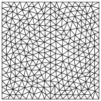
Figure 1: The triangulation of $\overline{\Omega}$ for $N=16$.

The initial value $(u_{h}^{0},p_{h}^{0})$ is set to be the Lagrange interpolation of $(u^{0},p^{0})$ in $\mathrm{P}_{k}/\mathrm{P}_{\ell}$-element space for Scheme$(k,\ell,\delta)$.

Remark 5.1.

Lagrange interpolation is sufficient for Hypothesis 4 in the velocity estimate (Section 3) but not for Hypothesis 6 in the pressure estimate (Section 4). For the effect to the pressure solution at the first step, see [8, 29].

Recall the norm notation in (16). The relative error $E_{X}$ is defined by

$$E_{X}(u)=\frac{\|u-\widetilde{u}_{h}\|_{X,h}}{\|u\|_{X,h}},\quad E_{X}(p)=\frac{\|p-p_{h}\|_{X,h}}{\|p\|_{X,h}},$$

where $X=\ell^{\infty}(L^{2})$ or $\ell^{2}(H_{0}^{1})$ for $u$, $X=\ell^{2}(L^{2})$ for $p$, and $\|\cdot\|_{X,h}$ means that the spatial norm is computed approximately by numerical quadrature of order nine [30]. Table 1 shows the symbols used in graphs. Since every graph of the relative error $E_{X}$ versus $h$ is depicted in the logarithmic scale, the slope corresponds to the convergence order.

Table 1: Symbols used in the graphs.

$\phi$	$u$	$u$	$p$
$X$	$\ell^{\infty}(L^{2})$	$\ell^{2}(H^{1}_{0})$	$\ell^{2}(L^{2})$
Scheme($2,1,0$)	$\blacktriangle$	$\bullet$	$\blacksquare$
Scheme($k,k,\delta$)	$\vartriangle$	$\circ$	$\square$

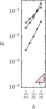
Figure 2: Relative errors versus $h$ for $\nu=1$. Scheme(2,1,0) with $\Delta t=h^{2}$ (left), Scheme(1,1,$10^{-1}$) with $\Delta t=(1/16)h$ (center), Scheme(2,2,$10^{-2}$) with $\Delta t=h^{2}$ (right).

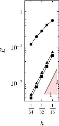
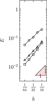
Figure 3: Relative errors versus $h$ for $\nu=10^{-4}$. Scheme(2,1,0) with $\Delta t=h^{2}$ (left), Scheme(1,1,$10^{-1}$) with $\Delta t=(1/16)h$ (center), Scheme(2,2,$10^{-2}$) with $\Delta t=h^{2}$ (right).

Figure 2 shows the graphs of the errors versus $h$ when $\nu=1$. For Scheme(2,1,0) and Scheme(2,2,$10^{-2}$), all convergence orders are almost two with no significant differences. For Scheme(1,1,$10^{-1}$), the convergence orders of $E_{\ell^{\infty}(L^{2})}(u)$ ($\vartriangle$) and $E_{\ell^{2}(L^{2})}(p)$ ($\square$) are greater than one. These exceed prediction from the theoretical result. Figure 3 shows the graphs when $\nu=10^{-4}$. For Scheme(2,1,0) and Scheme(2,2,$10^{-2}$), there are no significant difference in $E_{\ell^{\infty}(L^{2})}(u)$ ($\blacktriangle$,$\vartriangle$) and $E_{\ell^{2}(L^{2})}(p)$ ($\blacksquare$,$\square$). In Scheme(2,1,0), meanwhile, convergence order of $E_{\ell^{2}(H^{1}_{0})}(u)$ ($\bullet$) is about 0.8 to 1.4, which is less than 2. In Scheme(2,2,$10^{-2}$), convergence order of $E_{\ell^{2}(H^{1}_{0})}(u)$ ($\circ$) is about 1.5 to 1.8. To observe the convergence order $O(h^{2})$, finer meshes will be necessary. The error of Scheme(2,2,$10^{-2}$) ($\circ$) is almost ten times less than that of Scheme(2,1,0) ($\bullet$) for $h=1/64$. We also observe that the errors $E_{\ell^{2}(H^{1}_{0})}(u)$ of Scheme(1,1,$10^{-1}$) ($\circ$) is less than that of Scheme(2,1,0) ($\bullet$).

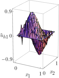
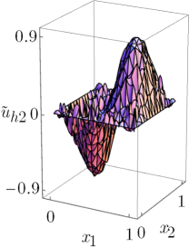
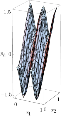
Figure 4: Stereographs of $\widetilde{u}_{h1}^{n},\widetilde{u}_{h2}^{n}$ and $p_{h}^{n}$ of Scheme(2,1,0), $\nu=10^{-4}$, $t^{n}=1$, $h=1/16$, $\Delta t=h^{2}$.

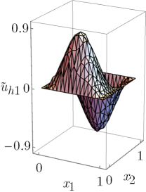
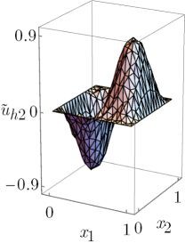
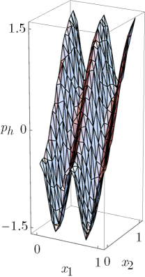
Figure 5: Stereographs of $\widetilde{u}_{h1}^{n},\widetilde{u}_{h2}^{n}$ and $p_{h}^{n}$ of Scheme(1,1,$10^{-1}$), $\nu=10^{-4}$, $t^{n}=1$, $h=1/16$, $\Delta t=(1/16)h$.

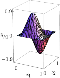
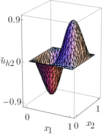
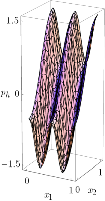
Figure 6: Stereographs of $\widetilde{u}_{h1}^{n},\widetilde{u}_{h2}^{n}$ and $p_{h}^{n}$ of Scheme(2,2,$10^{-2}$), $\nu=10^{-4}$, $t^{n}=1$, $h=1/16$, $\Delta t=h^{2}$.

Figures 4–6 show the stereographs of $\widetilde{u}_{h1}^{n}$, $\widetilde{u}_{h2}^{n}$ and $p_{h}^{n}$ when $\nu=10^{-4}$, $t^{n}=1$, $h=1/16$, and $\Delta t=1/256$. In Figure 4, we observe unnatural oscillation in the velocity of Scheme(2,1,0), which corresponds to the large error $E_{\ell^{2}(H^{1}_{0})}(u)$ ($\bullet$) in Figure 3. For the solutions of Scheme(1,1,$10^{-1}$) and Scheme(2,2,$10^{-2}$), we have no significant oscillation.

6 Concluding remarks

We developed and analyzed a pressure-stabilized projection LG scheme for the Oseen problem. The scheme inherits the advantages of computational efficiency from the projection/LG combined scheme. Here, since the viscosity term in the Oseen equations is Laplacian, the matrices can be decoupled into each component of the velocity and the pressure. We used the equal-order pair of the finite element for the velocity and pressure. Approximability of the pressure space is actually used in the velocity error estimate for small viscosity. We also derived the pressure error estimate, where the constant depends on the viscosity. Numerical results showed higher accuracy of the equal-order element than the Taylor–Hood element for small viscosity.

Appendix A Appendix

A.1 Proof of Lemma 4.8

Proof.

We prove (57). We apply Taylor’s theorem

$$g(1)=g(0)+g^{\prime}(0)+\frac{1}{2}g^{\prime\prime}(0)+\int_{0}^{1}\frac{(1-s)^{2}}{2}g^{\prime\prime\prime}(s)ds$$

to $g(s)=u(y_{j}(x,s),t_{j}(s))$ for $j=1,2$, where

$$(y_{j}(x,s),t_{j}(s))=(x-sw^{n-j}(x)\Delta t,t^{n-j+1}-s\Delta t)$$

so that $g(1)=(u^{n-j}\circ X_{1}(w^{n-j}))(x)$, $g(0)=u^{n-j+1}$, $g^{\prime}(0)=-\Delta tD_{w}^{n-j}u^{n-j+1}$ and $g^{\prime\prime}(0)=\Delta t^{2}(D_{w}^{n-j})^{2}u^{n-j+1}$. Here we have used the following material derivative

$$D_{w}^{n}:=\frac{\partial}{\partial t}+(w^{n}\cdot\nabla).$$

We have

$$R_{11}^{n}-R_{11}^{n-1}$$

$$= D_{w}^{n-1}u^{n}-\frac{u^{n}-u^{n-1}\circ X_{1}(w^{n-1})}{\Delta t}-\biggl{[}D_{w}^{n-2}u^{n-1}-\frac{u^{n-1}-u^{n-2}\circ X_{1}(w^{n-2})}{\Delta t}\biggr{]}$$

$$+[(w^{n}-w^{n-1})\cdot\nabla]u^{n}-[(w^{n-1}-w^{n-2})\cdot\nabla]u^{n-1}$$

$$= \frac{\Delta t}{2}(D_{w}^{n-1})^{2}u^{n}-\Delta t^{2}\int_{0}^{1}\frac{(1-s)^{2}}{2}(D_{w}^{n-1})^{3}u(y_{1}(\cdot,s),t_{1}(s))ds$$

$$-\frac{\Delta t}{2}(D_{w}^{n-2})^{2}u^{n-1}+\Delta t^{2}\int_{0}^{1}\frac{(1-s)^{2}}{2}(D_{w}^{n-2})^{3}u(y_{2}(\cdot,s),t_{2}(s))ds$$

$$+[(w^{n}-w^{n-1})\cdot\nabla]u^{n}-[(w^{n-1}-w^{n-2})\cdot\nabla]u^{n-1}.$$ (65)

We denote the $j$-th term in (65) by $R^{n}_{11j}$. We use (19) to have the following bound:

$$\|R^{n}_{111}-R^{n}_{113}\|_{0}\leq\frac{\Delta t^{3/2}}{2}\biggl{\|}\frac{\partial}{\partial t}\biggl{\{}\Bigl{[}\frac{\partial}{\partial t}+(w(\cdot-\Delta t)\cdot\nabla)\Bigr{]}^{2}u\biggr{\}}\biggr{\|}_{L^{2}(t^{n-1},t^{n};L^{2})}$$

$$\leq c(\|w\|_{W^{1,\infty}(L^{\infty})})\Delta t^{3/2}\|u\|_{Z^{3}(t^{n-1},t^{n})}.$$

For the second term,

$$\|R_{112}^{n}\|_{0} \leq\Delta t^{2}\int_{0}^{1}\biggl{\|}\frac{(1-s)^{2}}{2}\Bigl{(}\frac{\partial}{\partial t}+w^{n-1}\cdot\nabla\Bigr{)}^{3}u(y_{1}(\cdot,s),t_{1}(s))\biggr{\|}_{0}ds$$

$$\leq c(\|w^{n-1}\|_{0,\infty})\Delta t^{3/2}\|u\|_{Z^{3}(t^{n-1},t^{n})},$$

where we have used the transformation of independent variables from $x$ to $y$ and $s$ to $t$, and the estimate $|\det(\partial x/\partial y)|\leq 2$ by virtue of Lemma 3.4-(2). By the same argument

$$\|R_{114}^{n}\|_{0}\leq c(\|w^{n-2}\|_{0,\infty})\Delta t^{3/2}\|u\|_{Z^{3}(t^{n-2},t^{n-1})}.$$

For the fifth and the sixth term,

$$R_{115}^{n}-R_{116}^{n}$$

$$= \int_{t^{n-1}}^{t^{n}}\frac{\partial}{\partial t}\biggl{\{}\Bigl{[}(w(t)-w(t-\Delta t))\cdot\nabla\Bigr{]}u(t)\biggr{\}}dt$$

$$= \int_{t^{n-1}}^{t^{n}}\Bigl{[}(w_{t}(t)-w_{t}(t-\Delta t))\cdot\nabla\Bigr{]}u(t)dt+\int_{t^{n-1}}^{t^{n}}\Bigl{[}(w(t)-w(t-\Delta t))\cdot\nabla\Bigr{]}u_{t}(t)dt$$

$$= \int_{t^{n-1}}^{t^{n}}\Bigl{[}\int_{t-\Delta t}^{t}w_{tt}(s)ds\cdot\nabla\Bigr{]}u(t)dt+\int_{t^{n-1}}^{t^{n}}\Bigl{[}\int_{t-\Delta t}^{t}w_{t}(s)ds\cdot\nabla\Bigr{]}u_{t}(t)dt,$$

where $\Phi_{t}=\frac{\partial\Phi}{\partial t}$. Thus,

$$\|R_{115}^{n}-R_{116}^{n}\|_{0}\leq c(\|w\|_{W^{2,\infty}(L^{\infty})})\Delta t^{3/2}\|u\|_{H^{1}(t^{n-1},t^{n};H^{1})}.$$

Gathering these estimates, from (65), we have the conclusion (57).

We prove (58). First, we decompose the residual function as follows:

$$\frac{1}{\Delta t}[(v^{n}-v^{n-1}\circ X_{1}^{n-1})-(v^{n-1}-v^{n-2}\circ X_{1}^{n-1})]$$

$$-\frac{1}{\Delta t}[v^{n-2}\circ X_{1}^{n-1}-v^{n-2}\circ X_{1}^{n-2}]=:R^{n}_{41}-R^{n}_{42}.$$

Using $y(x,t,\tau):=x-w^{n-1}(x)(t-\tau)$, we have

$$R_{41}(x)= \frac{1}{\Delta t}\int_{t^{n-1}}^{t^{n}}\Bigl{[}v_{t}(x,t)-v_{t}(x-w^{n-1}(x)\Delta t,t-\Delta t)\Bigr{]}dt$$

$$= \frac{1}{\Delta t}\int_{t^{n-1}}^{t^{n}}\int_{t-\Delta t}^{t}D_{w}^{n-1}v_{t}(y(x,t,\tau),t)d\tau dt,$$

and thus

$$\|R_{41}\|_{0}\leq c\Delta t^{1/2}(\|v\|_{H^{2}(t^{n-2},t^{n};L^{2})}+\|w^{n-1}\|_{0,\infty}\|v\|_{H^{1}(t^{n-2},t^{n});H^{1}}).$$ (66)

Here, we have again used the transformation of independent variables from $x$ to $y$ and the estimate $|\det(\partial x/\partial y)|\leq 2$.

The bound for $R^{n}_{42}$ is easily obtained by Lemma 4.5 with $q=2$, $p=\infty$, $p^{\prime}=1$, $v=v^{n-2}$ and $w_{i}=w^{n-i}$, $i=1,2$:

$$\begin{split}\|R^{n}_{42}\|_{0}&\leq c\|\nabla v^{n-2}\|_{0}\|w^{n-1}-w^{n-2}\|_{0,\infty}\leq c\Delta t\|\nabla v^{n-2}\|_{0}\|w\|_{W^{1,\infty}(L^{\infty})}.\end{split}$$ (67)

The conclusion (58) follows from (66) and (67). ∎

Acknowledgment

The author was supported by Japan Society for the Promotion of Science under KAKENHI Grant Number JP18K13461.

References

- [1] Y. Achdou and J.-L. Guermond. Convergence analysis of a finite element projection/Lagrange–Galerkin method for the incompressible Navier–Stokes equations. SIAM Journal on Numerical Analysis, 37(3):799–826, 2000.
- [2] S. Badia and R. Codina. Convergence analysis of the FEM approximation of the first order projection method for incompressible flows with and without the inf-sup condition. Numerische Mathematik, 107(4):533–557, 2007.
- [3] R. Barrett, M. Berry, T. F. Chan, J. Demmel, J. Donato, J. Dongarra, V. Eijkhout, R. Pozo, C. Romine, and H. Van der Vorst. Templates for the Solution of Linear Systems: Building Blocks for Iterative Methods, 2nd Edition. SIAM, Philadelphia, PA, 1994.
- [4] M. Benítez and A. Bermúdez. A second order characteristics finite element scheme for natural convection problems. Journal of Computational and Applied Mathematics, 235(11):3270–3284, 2011.
- [5] F. Brezzi and J. Pitkäranta. On the stabilization of finite element approximations of the Stokes equations. In W. Hackbusch, editor, Efficient Solutions of Elliptic Systems, pages 11–19. Vieweg, 1984.
- [6] E. Burman. Pressure projection stabilizations for Galerkin approximations of Stokes’ and Darcy’s problem. Numerical Methods for Partial Differential Equations, 24(1):127–143, 2008.
- [7] E. Burman, A. Ern, and M. A. Fernández. Fractional-step methods and finite elements with symmetric stabilization for the transient Oseen problem. ESAIM: Mathematical Modelling and Numerical Analysis, 51(2):487–507, 2017.
- [8] E. Burman and M. A. Fernández. Galerkin finite element methods with symmetric pressure stabilization for the transient Stokes equations: Stability and convergence analysis. SIAM Journal on Numerical Analysis, 47(1):409–439, 2009.
- [9] G. Chen and M. Feng. Analysis of solving Galerkin finite element methods with symmetric pressure stabilization for the unsteady Navier-Stokes equations using conforming equal order interpolation. Advances in Applied Mathematics and Mechanics, 9(2):362–377, 2017.
- [10] P.G. Ciarlet. The Finite Element Method for Elliptic Problems, volume 40 of Classics in Applied Mathematics. SIAM, 2002.
- [11] Ph. Clément. Approximation by finite element functions using local regularization. RAIRO Analyse numérique, 9(R2):77–84, 1975.
- [12] J. de Frutos, B. García-Archilla, V. John, and J. Novo. Grad-div stabilization for the evolutionary Oseen problem with inf-sup stable finite elements. Journal of Scientific Computing, 66(3):991–1024, 2016.
- [13] J. de Frutos, B. García-Archilla, V. John, and J. Novo. Error analysis of non inf-sup stable discretizations of the time-dependent Navier–Stokes equations with local projection stabilization. IMA Journal of Numerical Analysis, 39(4):1747–1786, 2019.
- [14] J. de Frutos, B. García-Archilla, and J. Novo. Error analysis of projection methods for non inf-sup stable mixed finite elements: The Navier–Stokes equations. Journal of Scientific Computing, 74(1):426–455, 2018.
- [15] J. de Frutos, B. García-Archilla, and J. Novo. Error analysis of projection methods for non inf-sup stable mixed finite elements. The transient Stokes problem. Applied Mathematics and Computation, 322:154–173, 2018.
- [16] J. de Frutos, B. García-Archilla, and J. Novo. Fully discrete approximations to the time-dependent Navier–Stokes equations with a projection method in time and grad-div stabilization. Journal of Scientific Computing, 80(2):1330–1368, 2019.
- [17] J. de Frutos, B. García-Archilla, and J. Novo. Corrigenda: Fully discrete approximations to the time-dependent Navier–Stokes equations with a projection method in time and grad-div stabilization. Journal of Scientific Computing, 88(40), 2021.
- [18] J. Douglas, Jr. and T. Russell. Numerical methods for convection-dominated diffusion problems based on combining the method of characteristics with finite element or finite difference procedures. SIAM Journal on Numerical Analysis, 19(5):871–885, 1982.
- [19] L. P. Franca and T. J. R. Hughes. Two classes of mixed finite element methods. Computer Methods in Applied Mechanics and Engineering, 69(1):89–129, 1988.
- [20] L.P. Franca and R. Stenberg. Error analysis of some Galerkin least squares methods for the elasticity equations. SIAM Journal on Numerical Analysis, 28(6):1680–1697, 1991.
- [21] B. García-Archilla, V. John, and J. Novo. On the convergence order of the finite element error in the kinetic energy for high Reynolds number incompressible flows. Computer Methods in Applied Mechanics and Engineering, 385:114032, 2021.
- [22] B. García-Archilla, V. John, and J. Novo. Symmetric pressure stabilization for equal-order finite element approximations to the time-dependent Navier–Stokes equations. IMA Journal of Numerical Analysis, 41(2):1093–1129, 2021.
- [23] J.-L. Guermond. Some implementations of projection methods for Navier-Stokes equations. ESAIM: Mathematical Modelling and Numerical Analysis, 30(5):637–667, 1996.
- [24] J.-L. Guermond, P. Minev, and J. Shen. An overview of projection methods for incompressible flows. Computer Methods in Applied Mechanics and Engineering, 195:6011–6045, 2006.
- [25] J.-L. Guermond and P. D. Minev. Analysis of a projection/characteristic scheme for incompressible flow. Communications in Numerical Methods in Engineering, 19(7):535–550, 2003.
- [26] J.-L. Guermond and L. Quartapelle. On the aproximation of the unsteady Navier–Stokes equations by finite element projection methods. Numerische Mathematik, 80:207–238, 1998.
- [27] F. Hecht. New development in FreeFem++. Journal of Numerical Mathematics, 20(3-4):251–265, 2012.
- [28] J. G. Heywood and R. Rannacher. Finite-element approximation of the nonstationary Navier-Stokes problem. Part IV: Error analysis for second-order time discretization. SIAM Journal on Numerical Analysis, 27(2):353–384, 1990.
- [29] V. John and J. Novo. Analysis of the pressure stabilized Petrov–Galerkin method for the evolutionary Stokes equations avoiding time step restrictions. SIAM Journal on Numerical Analysis, 53(2):1005–1031, 2015.
- [30] M. E. Laursen and M. Gellert. Some criteria for numerically integrated matrices and quadrature formulas for triangles. International Journal for Numerical Methods in Engineering, 12(1):67–76, 1978.
- [31] A. Linke and L. G. Rebholz. On a reduced sparsity stabilization of grad-div type for incompressible flow problems. Computer Methods in Applied Mechanics and Engineering, 261-262:142–153, 2013.
- [32] M. Lukáčová-Medvid’ová, H. Mizerová, H. Notsu, and M. Tabata. Numerical analysis of the Oseen-type Peterlin viscoelastic model by the stabilized Lagrange-Galerkin method. Part I: A nonlinear scheme. ESAIM: Mathematical Modelling and Numerical Analysis, 51(5):1637–1661, 2017.
- [33] M. Lukáčová-Medvid’ová, H. Mizerová, H. Notsu, and M. Tabata. Numerical analysis of the Oseen-type Peterlin viscoelastic model by the stabilized Lagrange-Galerkin method. Part II: A linear scheme. ESAIM: Mathematical Modelling and Numerical Analysis, 51(5):1663–1689, 2017.
- [34] A. Misawa. Error estimates of an Euler approximated characteristics/projection finite element scheme for the incompressible Navier–Stokes equations and its application. Master’s thesis, Waseda University, Japan, 2016. In Japanese.
- [35] H. Notsu and M. Tabata. Error estimates of a pressure-stabilized characteristics finite element scheme for the Oseen equations. Journal of Scientific Computing, 65(3):940–955, 2015.
- [36] M.A. Olshanskii and A. Reusken. Grad-div stablilization for Stokes equations. Mathematics of Computation, 73:1699–1718, 2004.
- [37] O. Pironneau. On the transport-diffusion algorithm and its applications to the Navier-Stokes equations. Numerische Mathematik, 38:309–332, 1982.
- [38] H. Rui and M. Tabata. A second order characteristic finite element scheme for convection-diffusion problems. Numerische Mathematik, 92:161–177, 2002.
- [39] E. Süli. Convergence and nonlinear stability of the Lagrange-Galerkin method for the Navier-Stokes equations. Numerische Mathematik, 53(4):459–483, 1988.
- [40] M. Tabata and S. Uchiumi. An exactly computable Lagrange–Galerkin scheme for the Navier–Stokes equations and its error estimates. Mathematics of Computation, 87(309):39–67, 2018.
- [41] K. Tanaka, A. Suzuki, and M. Tabata. A characteristic finite element method using the exact integration. Annual Report of Research Institute for Information Technology of Kyushu University, 2:11–18, 2002. (Japanese).
- [42] S. Uchiumi. A viscosity-independent error estimate of a pressure-stabilized Lagrange–Galerkin scheme for the Oseen problem. Journal of Scientific Computing, 80(2):834–858, 2019.