Exponential escape efficiency of SGD from sharp minima in non-stationary regime

Abstract

We show that stochastic gradient descent (SGD) escapes from sharp minima exponentially fast even before SGD reaches stationary distribution. SGD has been a de-facto standard training algorithm for various machine learning tasks. However, there still exists an open question as to why SGDs find highly generalizable parameters from non-convex target functions, such as the loss function of neural networks. An “escape efficiency” has been an attractive notion to tackle this question, which measures how SGD efficiently escapes from sharp minima with potentially low generalization performance. Despite its importance, the notion has the limitation that it works only when SGD reaches a stationary distribution after sufficient updates. In this paper, we develop a new theory to investigate escape efficiency of SGD with Gaussian noise, by introducing the Large Deviation Theory for dynamical systems. Based on the theory, we prove that the fast escape form sharp minima, named exponential escape, occurs in a non-stationary setting, and that it holds not only for continuous SGD but also for discrete SGD. A key notion for the result is a quantity called “steepness,” which describes the SGD’s stochastic behavior throughout its training process. Our experiments are consistent with our theory.

Keywords Deep learning  $\cdot$ Stochastic gradient descent  $\cdot$ Flat minima

1 Introduction

Stochastic gradient descent (SGD) has become the de facto standard optimizer in modern machine learning, especially deep learning. However, its prevalence has opened up a theoretical question: why can SGD find generalizable solutions in complicated models such as neural networks? The loss landscapes of neural networks are known to be highly non-convex (Li et al., 2018), difficult to minimize (Blum and Rivest, 1992), and full of non-generalizable minima (Zhang et al., 2017). It is an important task to answer this open question to attain a solid understanding of modern machine learning.

In recent years, “escape efficiency from sharp minima” has emerged as a promising narrative for the SGD’s generalization. “Sharp minima” mean the model parameters as local minima of loss functions and that are sensitive to perturbations. They are known to deteriorate generalization ability by several empirical and theoretical studies (Keskar et al., 2016; Dziugaite and Roy, 2017; Jiang et al., 2019). The “escape efficiency,” the counterpart of the narrative, is a measure for how fast SGD moves out of the neighborhood of minima. In a few words, the narrative claims that SGD can find generalizable minima because it has high escape efficiency from sharp minima (Zhu et al., 2018; Xie et al., 2020). This narrative is aligned with actual phenomena. The left panel of Fig. 1 shows how SGD updates affect sharpness of parameters throughout the training of a neural network, where the sharpness oscillates widely in the early phase of the training, and then becomes smaller toward the end. This suggests that SGD repeatedly jumps out of sharp minima and eventually reaches flat minima (Fig. 1, right).

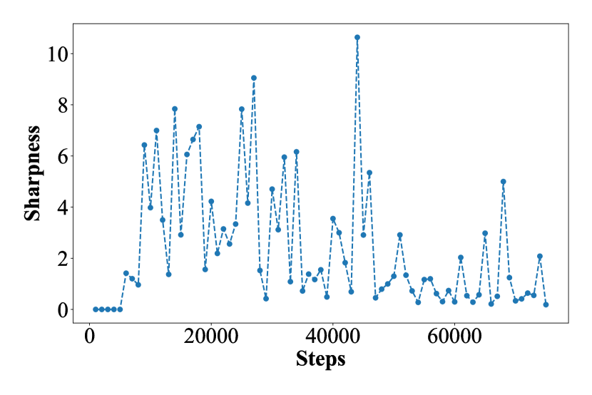
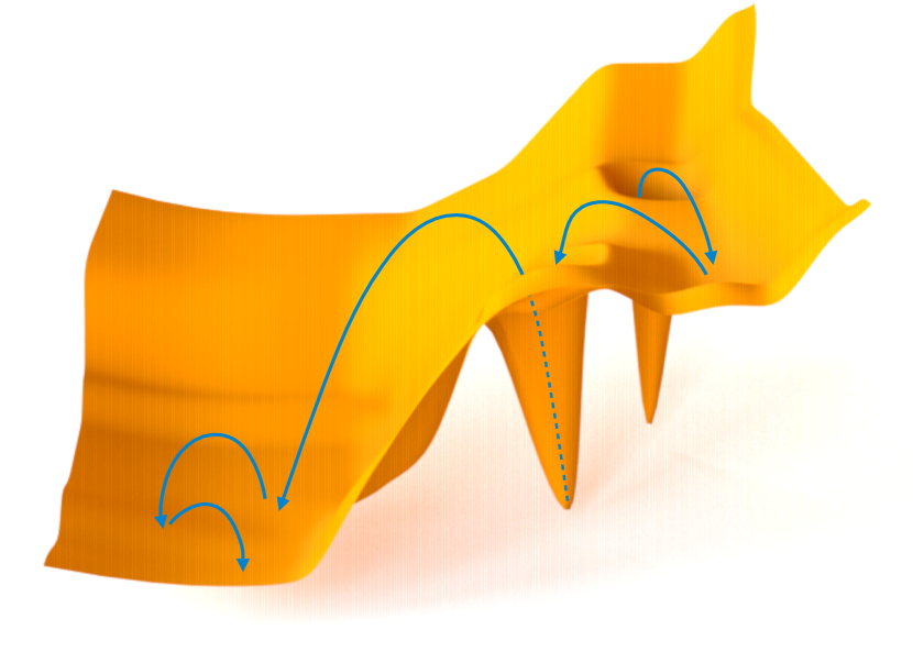
Figure 1: Sharpness dynamics throughout a training via SGD (left), where we used the sharpness defined in (Keskar et al., 2016, Metric 2.1). As is shown, sharpness fluctuates during the training and becomes small toward the end of training. This means SGD jumps out from sharp minima to find flat and generalizable minima (right). We used VGG (Simonyan and Zisserman, 2014) fed with CIFAR-10 (Krizhevsky et al., 2009) with cross entropy loss.

Many theoretical studies have investigated the escape efficiency to quantify SGD’s escaping behavior. Regarding SGD as a gradient descent with noise, recent studies have identified that the noise part plays a key role in escaping. It was shown that high escape efficiency is realized by the so-called “anisotropic noise” of SGD, which means the noise with the various magnitudes among directions (Zhu et al., 2018). Jastrzębski et al. (2017) formulated the effect of anisotropic noise in the stationary regime, where SGD has reached a stationary distribution after many iterations. By limiting the target to the stationary regime, they took advantage of the theoretical analogy between SGD and thermodynamics. Xie et al. (2020) further elaborated this approach and found that escape efficiency can be viewed as Kramer’s escape rate, which is a well-used formula in various fields of science (Kramers, 1940). Their result revealed that SGD has the “exponential escape efficiency” from sharp minima, which means the sharpness exponentially increases SGD’s escape efficiency.

With these progressive refinements, a remaining task is how to go beyond the stationary regime. Although physics and chemistry commonly assume that a system has reached a stationary distribution (Eyring, 1935; Hanggi, 1986), the stationary regime does not apply to the analysis of SGD due to the following reasons. First, it is shown that SGD forms a stationary distribution only on the very limited objective functions (Dieuleveut et al., 2017; Chen et al., 2021). Secondly, even when such a stationary distribution exists, SGD takes $O(d)$ steps to reach it, where $d$ is a number of parameters of a model (Raginsky et al., 2017). Since common neural networks have numerous parameters, the stationary regime may not be directly applicable to the actual SGD dynamics.

In this paper, we propose a novel formulation of exponential escape efficiency of SGD with Gaussian noise in the non-stationary regime, by introducing the Large Deviation Theory (Freidlin and Wentzell, 2012; Dembo and Zeitouni, 2010), a fundamental theory of stochastic systems. We formulate the escape efficiency of SGD through a notion of “steepness,” which intuitively means the hardness to climb up loss surface along a given trajectory (Fig. 2). Large Deviation Theory provides that the escape efficiency is described by steepness of a trajectory starting from the minimum:

$$\textrm{Escape efficiency}\sim\exp{\left[-V_{0}\right]}\quad(V_{0}:\textrm{steepness from a minimum})$$

Based on this analysis, we show the following main result on the escape efficiency of SGD:

Theorem 2 (informal): Escape efficiency of SGD $$\sim\exp\left[-\frac{B}{\eta}\Delta L\lambda^{-\frac{1}{2}}_{\mathrm{max}}\right],$$

where $B$ is a batch size, $\eta$ is a learning rate, $\Delta L$ is the depth of the minimum, and $\lambda_{\mathrm{max}}$ is the sharpness of a loss function (Definition 3). We can see that as sharpness of the minimum increases, i.e. $\lambda_{\max}$ increases, the escape efficiency increases exponentially. This is the first result showing that SGD has exponential escape efficiency from sharp minima, even out of the stationary regime. As a further benefit, our formulation can be easily extended to the discrete update rule of SGD (Theorem 3).

Figure 2: Visual illustration of steepness (Definition 4). The steepness of $\varphi$, $S_{T}(\varphi)$, is greater than $S_{T}(\psi)$ because $\varphi$ moves against the vector field of gradient $-\nabla L(\theta)$.

The rest of this paper is organized as follows. Section 2 formulates the SGD’s escape problem. Section 3 presents the traditional Large Deviation Theory and its application to the SGD’s escape problem. Section 4 gives the main results on the escape efficiency. In Section 5, we confirm that the main results are consistent with numerical experiments.

2 Problem Formulation

Notations: For a $k\times k$ matrix $A$, $\lambda_{j}(A)$ is the $j$-th largest eigenvalue of $A$. We especially write $\lambda_{\max}(A)=\lambda_{1}(A)$ and $\lambda_{\min}(A)=\lambda_{k}(A)$. $\mathcal{O}(\cdot)$ denotes Landau’s Big-O notation. $\|\cdot\|$ denotes the Euclidean norm. Given a time-dependent function $\theta_{t}$, $\dot{\theta}_{t}$ denotes the differentiation of $\theta_{t}$ with respect to $t$. $N\left(\mu,\Sigma\right)$ denotes the multivariate Gaussian distribution with the mean $\mu$, and the covariance $\Sigma$.

2.1 Stochastic Gradient Descents

We consider a learning model parameterized by $\theta\in\mathbb{R}^{d}$, where $d$ is a number of parameters. Given training examples $\{x_{i}\}_{i=1}^{N}$ and a loss function $\ell(\theta,x_{i})$, we consider a training loss $L(\theta):=\frac{1}{N}\sum_{i=1}^{N}\ell(\theta,x_{i})$ and a mini-batch loss $L^{B}(\theta):=\frac{1}{B}\sum_{x_{i}\in\mathcal{B}}\ell(\theta,x_{i})$, where $\mathcal{B}$ is a randomly sampled subset of the training data such that $|\mathcal{B}|=B$. With a minimum $\theta^{*}\in\mathbb{R}^{d}$, we define $\Delta L:=\min_{\theta\in\partial D}L(\theta)-L(\theta^{*})$ as a depth of a loss function around $\theta^{*}$.

We consider two types of stochastic gradient descent (SGD) methods; a discrete SGD and a continuous SGD. Although the ordinary SGD is discrete, we focus on its continuous variation for mathematical convenience.

Discrete SGD: Given an initial parameter $\theta_{0}\in\mathbb{R}^{d}$ and a learning rate $\eta>0$, SGD generates a sequence of parameters $\{\theta_{k}\}_{k\in\mathbb{N}}$ by the following update rule:

$$\theta_{k+1}=\theta_{k}-\eta\nabla L^{B}(\theta_{k}),~{}k\in\mathbb{N}.$$ (1)

We model SGD as a gradient descent with a Gaussian noise perturbation. We decompose $-\nabla L^{B}(\theta_{k})$ in (1) into a gradient term $-\nabla L(\theta_{k})$ and a noise term $\nabla L(\theta_{k})-\nabla L^{B}(\theta_{k})$, and model the noise as a Gaussian noise. With this setting, the update rule in (1) is rewritten as

$$\theta_{k+1}=\theta_{k}-\eta\nabla L(\theta_{k})+\sqrt{\frac{\eta}{B}}W_{k},$$ (2)

where $W_{k}\sim N\left(0,\eta C(\theta_{k})\right)$ is a parameter-dependent Gaussian noise with its covariance. Note that $\eta$ appears in both the covariance $\eta C(\theta_{k})$ and the coefficient $\sqrt{\eta/B}$ of the noise $W_{k}$, because it is useful to make the connection with the subsequent continuous SGD clear.

The Gaussianity of the noise on gradients is justified by the following reasons: (i) if the batch size $B$ is sufficiently large, the central limit theorem ensures the noise term becomes Gaussian, and (ii) several empirical studies show that the noise term follows Gaussian distribution (Mandt et al., 2016; Jastrzębski et al., 2017; He et al., 2019a).

Continuous SGD: We formulate a continuous SGD such that its discretization corresponds to the discrete SGD (2) based on the Euler scheme (e.g. Definition 5.1.1 of Gobet (2016)). With a time index $t\geq 0$ and the given initial parameter $\theta_{0}\in\mathbb{R}^{d}$, the continuous dynamic of SGD is written as the following system:

$$\dot{\theta}_{t} =-\nabla L(\theta_{t})+\sqrt{\frac{\eta}{B}}{C(\theta_{t})}^{1/2}\dot{w}_{t}$$ (3)

where $w_{t}$ is a $d$-dimensional Wiener process, i.e. an $\mathbb{R}^{d}$-valued stochastic process with $t$ such that $w_{0}=0$ and $w_{t+u}-w_{t}\sim N(0,uI)$ for any $t,u>0$. We note that this system can be seen as a Gaussian perturbed dynamical system with a noise magnitude $\sqrt{{\eta}/{B}}$ because $\eta$ and $B$ do not evolve by time.

2.2 Mean Exit Time

We consider the problem on how discrete and continuous SGD’s escape from minima of loss surfaces. This is formally quantified by a notion of mean exit time. We define $\theta^{*}\in\mathbb{R}^{d}$ as a local minimum of loss surfaces, and also define its neighborhood $D\subset\mathbb{R}^{d}$ as an open set which contains $\theta^{*}$. We define the mean exit time as follows:

Definition 1 (Mean exit time from $D$).

Consider a continuous SGD (3) starting from $\theta_{0}\in D$. Then, a mean exit time of the continuous SGD from $D$ is defined as

$$\mathbb{E}[\tau]:=\mathbb{E}[\min\left\{t:\theta_{t}\notin D\right\}].$$

Intuitively, a continuous SGD with small $\mathbb{E}[\tau]$ easily escapes from the neighbourhood $D$.

Similarly, we define the discrete mean exit time as follows. Here, a product of the learning rate $\eta$ and the update index $k$ plays a role of the time index $t$, since the $\eta$ is regarded as a width of the discretization.

Definition 2 (Discrete mean exit time from $D$).

Consider a discrete SGD (2) starting from $\theta_{0}\in D$. Then, a discrete mean exit time of the discrete SGD from $D$ is defined as

$$\mathbb{E}[\nu]:=\mathbb{E}[\min\left\{k\eta:\theta_{k}\notin D\right\}].$$

In our study, we measure the escape efficiency by an inverse of the notion of mean exit time. Rigorously, we consider the following definition:

$$\text{Escape efficiency}:=\text{(Mean exit time)}^{-1}.$$

Remark 1 (Other measures on escape).

There exist several terms in the machine learning community that represent similar notions. The term “escaping efficiency” was first defined by Zhu et al. (2018) as $\mathbb{E}_{\theta_{t}}\left[L\left(\theta_{t}\right)-L\left(\theta_{0}\right)\right]$. Xie et al. (2020) defined an “escape rate” as a ratio between the probability of coming out from $\theta^{*}$’s neighborhood and the probability mass around $\theta^{*}$. They also defined an “escape time” by the inverse of the escape rate.

2.3 Setting and Basic Assumptions for SGD’s Escape Problem

We provide basic assumptions that are commonly used in the literature of the escape problem (Mandt et al., 2016; Zhu et al., 2018; Jastrzębski et al., 2017; Xie et al., 2020).

Assumption 1 ($L(\theta)$ is locally quadratic in $D$).

There exists a matrix $H^{*}\in\mathbb{R}^{d\times d}$ such that for any $\theta\in D$, the following equality holds:

$$\forall\theta\in D,L(\theta)=L\left(\theta^{*}\right)+\nabla L\left(\theta^{*}\right)\left(\theta-\theta^{*}\right)+\frac{1}{2}\left(\theta-\theta^{*}\right)^{\top}H^{*}\left(\theta-\theta^{*}\right)$$

Assumption 2 (Hesse covariance matrix).

For any $\theta\in D$, $C(\theta)$ is approximately equal to $H^{*}$.

It is known that Assumption 2 holds when $\theta^{*}$ is a critical point (Zhu et al., 2018; Jastrzębski et al., 2017). It is also empirically shown that Assumption 2 can approximately hold even for randomly chosen $\theta$ (see Section 2 of Xie et al. (2020)).

Finally, we use the following definition as sharpness in our analysis.

Definition 3 (Sharpness of a minimum $\theta^{*}$).

Sharpness of $\theta^{*}$ is the maximum eigenvalue of $H^{*}$ in Assumption 1, that is,

$$\lambda_{\max}=\lambda_{\max}(H^{*}).$$

This is one of the most common definitions of sharpness (Jastrzebski et al., 2020), although the definition of sharpness is a controversial topic by itself (Dinh et al., 2017),

3 Large Deviation Theory for SGD

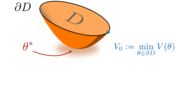
Figure 3: Notions related to the fundamental theorem (Theorem 1), a minimum $\theta^{*}$, its neighborhood hood $D$ as well as the boundary $\partial D$, and $V_{0}$, which is defined as the smallest quasi-potential in $\partial D$.

We introduce the basic notions from the Large Deviation Theory (Freidlin and Wentzell, 2012; Dembo and Zeitouni, 2010).

First, we define steepness of a trajectory on a loss surface $L(\theta)$, followed by the continuous SGD (3). Let $\varphi=\{\varphi_{t}\}_{t\in[0,T]}\subset\mathbb{R}^{d}$ be a trajectory in the parameter space over a time interval $[0,T]$ with a terminal time $T$, where $\varphi_{t}\in\mathbb{R}^{d}$ is a parameter which continuously changes in $t$ (see Figure 2). Also, $\varphi$ is regarded as a continuous map from $[0,T]$ to $\mathbb{R}^{d}$, i.e. is an element of $\mathbf{C}_{T}(\mathbb{R}^{d})$ (a set of continuous trajectories in $\mathbb{R}^{d}$) which is a support of continuous SGD during $[0,T]$. Given a trajectory $\varphi$ and the system (3), we define the following quantity:

Definition 4 (Steepness of $\varphi$).

Steepness of a trajectory $\varphi$ followed by (3) is defined as

$$S_{T}(\varphi):=\frac{1}{2}\int_{0}^{T}\left(\dot{\varphi}_{t}+\nabla L\left(\varphi_{t}\right)\right)^{\top}C\left(\varphi_{t}\right)^{-1/2}\left(\dot{\varphi}_{t}+\nabla L\left(\varphi_{t}\right)\right)dt.$$

Intuitively, steepness $S_{T}(\varphi)$ is interpreted as the hardness for the system (3) to follow this trajectory $\varphi$ up the hill on $L(\theta)$, as illustrated in Figure 2. This notion is generally utilized in the Large Deviation Theory, and is called “normalized action functional” in Freidlin and Wentzell (2012, Section 3.2) or “rate function” in Dembo and Zeitouni (2010, Section 1.2).

Steepness is a useful measure to formally describe a distribution of trajectories generated by continuous SGD. If a trajectory $\varphi$ has a large steepness $S_{T}(\varphi)$, the probability that the system takes the trajectory decreases exponentially. Formally, the distributions are described as follows. $\mathrm{P}_{\varphi^{\prime\prime}}\left(\cdot\right)$ is a distribution of a (random) trajectory $\varphi^{\prime\prime}$ generated from the continuous SGD (3).

Lemma 1 (Theorem 3.1 in Freidlin and Wentzell (2012)).

For any $\delta,\zeta>0$ and $\varphi\in\mathbf{C}_{T}\left(\mathbb{R}^{d}\right)$, there exists $\varepsilon=\varepsilon(\delta,\zeta)>0$ such that the following holds:

$$\mathrm{P}_{\varphi^{\prime\prime}}\left(\varphi^{\prime\prime}\in\left\{\varphi^{\prime}\in\mathbf{C}_{T}(\mathbb{R}^{d})\mid\rho\left(\varphi^{\prime},\varphi\right)<\delta\right\}\right)\geq\exp\left\{-\varepsilon^{-2}\left[S_{T}\left(\varphi\right)+\zeta\right]\right\},$$

where $\rho(\varphi^{\prime},\varphi)=\sup_{t\in[0,T]}\|\varphi^{\prime}_{t}-\varphi_{t}\|$.

Lemma 2 (Theorem 3.1 in Freidlin and Wentzell (2012)).

Let $\Phi(s)=\left\{\varphi\in\mathbf{C}_{T}(\mathbb{R}^{d})\mid S_{T}(\varphi)\leq s\right\}$. For any $\delta,\zeta$ and $s>0$, there exists $\varepsilon=\varepsilon(\delta,\zeta,s)>0$ such that the following holds:

$$\mathrm{P}_{\varphi^{\prime\prime}}\Big{(}\varphi^{\prime\prime}\in\left\{\varphi^{\prime}\in\mathbf{C}_{T}(\mathbb{R}^{d})\mid\rho(\varphi^{\prime},\Phi(s))\geq\delta\right\}\Big{)}\leq\exp\{-\varepsilon^{-2}(s-\zeta)\},$$

where $\rho(\varphi^{\prime},\Phi(s))=\inf_{\varphi\in\Phi(s)}\rho(\varphi^{\prime},\varphi)$.

Although we focus on the continuous SGD, similar discussions are applicable to a general class of diffusion processes (Dembo and Zeitouni, 2010, Section 5.7) and systems with Markov perturbations (Freidlin and Wentzell, 2012, Section 6.5).

We secondly define quasi-potential, which is the smallest steepness from a minimum $\theta^{*}$ to a boundary $\partial D$. It plays an essential role in the mean exit time.

Definition 5 (Quasi-potential).

Given the system (3) whose initial point is a local minima $\theta^{*}$, quasi-potential of a parameter $\theta\in D$ is defined as

$$V(\theta):=\inf_{T>0}\inf_{\varphi:\begin{subarray}{c}(\varphi_{0},\varphi_{T})=(\theta^{*},\theta)\end{subarray}}S_{T}(\varphi).$$

Same as steepness, quasi-potential can be seen as the minimum effort the system (3) needs to climb from $\theta^{*}$ up to $\theta$ on $L(\theta)$. (For more details, see Freidlin and Wentzell (2012, Section 5.3)).

We describe the mean exit time of a continuous SGD (3) based on the notion of quasi-potential. We obtain the following theorem by applying the fundamental results of Large Deviation Theory:

Theorem 1 (Fundamental Theorem).

Consider the continuous SGD (3) whose initial point is the local minima $\theta_{0}=\theta^{*}$. Suppose Assumption 1 holds. Then, the mean exit time (Definition 1) has the following limit:

$$\lim_{\eta\to 0}\frac{\eta}{B}\ln\mathbb{E}\left[\tau\right]=V_{0}$$

holds, where $V_{0}:=\min_{\theta\in\partial D}V(\theta)$.

We obtain Theorem 1 by adapting a general theorem in (Freidlin and Wentzell, 2012, Section 4) to our setting with Assumption 1. Rigorously, we verify that several requirements of the general theorem, such as asymptotic stability and attractiveness, are satisfied with our setup. The precise description of the assumptions can be found in Appendix A, and the proof of Theorem 1 under our setup in Appendix B.

4 Mean Exit Time Analysis

In this section, we give an asymptotic analysis of the mean exit time as our main result. As preparation, we provide an approximate computation of the quasi-potential in our setting, then we give the main theorem.

4.1 Approximate Computation of Quasi-potential

We develop an approximation of the quasi-potential $V(\theta)$, which is necessary to study the mean exit time by the fundamental theorem (Theorem 1). However, the direct calculation with a general $C(\theta)$ is a difficult problem, and at best we get a necessary condition for the exact formula (Appendix C). Instead, we consider a proximal system which is a simplified version of the continuous SGD (3) with a state-independent noise covariance.

4.1.1 Proximal System with $C(\theta)=I$

We define the following proximal system which generates a sequence $\{\hat{\theta}_{t}\}$:

$$\dot{\hat{\theta}}_{t}=-\nabla L\left(\hat{\theta}_{t}\right)+\sqrt{\frac{\eta}{B}}\dot{w}_{t}$$ (4)

This system is obtained by replacing the covariance $C(\theta)$ of the continuous SGD (3) into an identity $I$. That is, this proximal system is regarded as a Gaussian gradient descent with isotropic noise.

We further define steepness and quasi-potential of the proximal system as follow:

$$\textbf{Steepness}\quad\text{For each $\varphi\in\mathbf{C}_{T}(\mathbb{R}^{d})$, }\hat{S}_{T}(\varphi):=\frac{1}{2}\int_{0}^{T}\|\dot{\varphi}_{t}+\nabla L\left(\varphi_{t}\right)\|^{2}dt$$ (5)

$$\textbf{Quasi-potential}\quad\text{For each $\theta\in D$, }\hat{V}(\theta):=\inf_{T>0}\inf_{\varphi:\left(\varphi_{0},\phi_{r}\right)=\left(\theta^{*},\theta\right)}\hat{S}_{T}(\varphi)$$ (6)

Owing to the noise structure of the proximal system, we achieve an simple form of the quasi-potential. For the quasi-potential $\hat{V}(\theta)$, the following lemma holds:

Lemma 3.

Under Assumption 1, $\hat{V}(\theta)=2\left(L(\theta)-L(\theta^{*})\right)$.

Proof.

If the function $\varphi_{t}$ for $t\in\left[0,T\right]$ does not exit from $D\cup\partial D$,

$$\hat{S}_{T}(\varphi) =\frac{1}{2}\int_{0}^{T}\left\|\dot{\varphi}_{t}-\nabla L\left(\varphi_{t}\right)\right\|^{2}dt+2\int_{0}^{T}\dot{\varphi}_{t}^{\top}\nabla L\left(\varphi_{t}\right)dt$$

$$=\frac{1}{2}\int_{0}^{T}\left\|\dot{\varphi}_{t}-\nabla L\left(\varphi_{t}\right)\right\|^{2}dt+2\left(L(\varphi_{T})-L(\varphi_{0})\right)$$

$$\geq 2\left(L(\varphi_{t})-L(\varphi_{0})\right)$$

The equality holds when $\dot{\varphi}_{t}=\nabla L\left(\varphi_{t}\right)$. Since quasi-potential at $\theta$ is the infimum of the steepness from $\theta^{*}$ to $\theta$, $\hat{V}(\theta)=2\left(L(\theta)-L(\theta^{*})\right)$ is obtained. ∎

Lemma 3 shows that the quasi-potential with the proximal system is simply represented as the height of $\theta$ from a minimum $\theta^{*}$. By the quasi-potential, we simply obtain the following result by combining Theorem 1:

Proposition 1 (Mean Exit Time of Proximal System).

Consider the proxy system (4) whose initial point is the local minima $\theta_{0}=\theta^{*}$. Suppose that Assumption 1, 2, and 3 hold. Then, the mean exit time of (4) from the neighborhood $D$, $\mathbb{E}[\hat{\tau}]$, has the following limit

$$\lim_{\eta\to 0}\frac{\eta}{B}\ln\mathbb{E}[\hat{\tau}]=\Delta L.$$

4.1.2 Approximation of Quasi-potential $V_{0}:=\min_{\theta\in\partial D}V(\theta)$

We approximate the target quasi-potential $V(\theta)$ using $\lambda_{\mathrm{max}}^{-{1}/{2}}\hat{V}(\theta)$ from the proximal system. For this sake, we impose the following assumption:

Assumption 3.

There exists $K>0$ such that for any $\varphi\in\mathbf{C}_{T}\left(\mathbb{R}^{d}\right)$ and $t\in[0,T]$, $\dot{\varphi}_{t}\leq K$ holds.

This claims that the velocities of trajectories do not become infinitely large. With this mild assumption, we obtain the estimation of $V_{0}$ as follows. We define that $\kappa$ is the condition number of $C(\theta^{*}):=\lambda_{\max}/\lambda_{\min}$.

Lemma 4.

Under Assumption 1, 2, and 3, there exists a constant $A$ such that

$$\left|V_{0}-\lambda_{\mathrm{max}}^{-\frac{1}{2}}\hat{V}_{0}\right|\leq A\lambda_{\mathrm{min}}^{\frac{1}{2}}\left(\kappa^{\frac{1}{2}}-1\right).$$

This lemma implies that the quasi-potential of continuous SGD is approximated by $\lambda_{\mathrm{max}}^{-{1}/{2}}\hat{V}_{0}$. When $\lambda_{\mathrm{max}}>1$ holds, continuous SGD has smaller quasi-potential than that of the proximal system. We can see that the tightness of the approximation is described by by the degree of “anisotropy” of the noise (i.e. $\kappa$), since the bound $A\lambda_{\mathrm{min}}^{{1}/{2}}(\kappa^{{1}/{2}}-1)$ is mainly determined $\lambda_{\mathrm{max}}$.

4.2 Main Results: Mean Exit Time Analysis

As our main results, we give inequalities that characterize a limit of the mean escape time. We recall the definition of the depth of a minimum $\theta^{*}$ as $\Delta L:=\min_{\theta\in\partial D}L(\theta)-L(\theta^{*})$.

Continuous SGD

First, we study the case of continuous SGD (3). This result is obtained immediately by combining the fundamental theorem (Theorem 1) with the approximated quasi-potential (Lemma 4):

Theorem 2 (Mean Exit Time of Continuous SGD).

Consider the continuous SGD (3) whose initial point is the local minima $\theta_{0}=\theta^{*}$. Suppose that Assumption 1, 2, and 3 hold. Then, the mean exit time (Definition 1) from the neighbourhood $D$ has the following limit:

$$2\lambda_{\mathrm{max}}^{-\frac{1}{2}}\Delta L-A\lambda_{\mathrm{min}}^{\frac{1}{2}}\left(\kappa^{\frac{1}{2}}-1\right)\leq \lim_{\eta\to 0}\frac{\eta}{B}\ln\mathbb{E}[\tau]\leq 2\lambda_{\mathrm{max}}^{-\frac{1}{2}}\Delta L+A\lambda_{\mathrm{min}}^{\frac{1}{2}}\left(\kappa^{\frac{1}{2}}-1\right).$$

Excluding the effect of the approximation $A\lambda_{\mathrm{min}}^{{1}/{2}}(\kappa^{{1}/{2}}-1)$, this result indicates that continuous SGD needs $\exp(2\frac{B}{\eta}\Delta L\lambda_{\mathrm{max}}^{-{1}/{2}})$ number of steps asymptotically, before escaping from the neighborhood $D$ of the local minima $\theta^{*}$. Compared to the quasi-potential of the proxy system $2\Delta L$ (Proposition 1), the covariance matrix reduces quasi-potential in the factor of $\lambda_{\mathrm{max}}^{{1}/{2}}$. This result endorses the fact that SGD’s noise structure, $C(\theta)$, exponentially accelerates the escaping (Xie et al., 2020), because quasi-potential exponentially affect mean exit time (Theorem 1). A more rigorous comparison is given in Section 6.

Discrete SGD

Next, we give the mean escape time analysis for discrete SGD (2). Our approach is to combine the following discretization error analysis to the continuous SGD results (Theorem 2):

Lemma 5 (Discretization Error).

For a stochastic system with Gaussian perturbation and its discrete correspondence, the discretization error of exit time has the following convergence rate

$$\mathbb{E}[\nu]-\mathbb{E}[\tau]=\mathcal{O}(\sqrt{\eta}).$$

The following lemma can be simply derived as a special case of (Gobet and Menozzi, 2010, Theorem 17) by substituting $g(\cdot)=0,f(\cdot)=1,$ and $k(\cdot)=0$ in their definition.

Based on the analysis, we obtain the following result:

Theorem 3 (Mean Exit Time of Discrete SGD).

Consider the discrete Gaussian SGD (2) whose initial point is the local minima $\theta_{0}=\theta^{*}$. Suppose that Assumption 1, 2, and 3, hold. Then, the mean exit time (Definition 1) from the neighbourhood $D$ has the following limit:

$$2\lambda_{\mathrm{max}}^{-\frac{1}{2}}\Delta L-A\lambda_{\mathrm{min}}^{\frac{1}{2}}\left(\kappa^{\frac{1}{2}}-1\right)\leq \lim_{\eta\to 0}\frac{\eta}{B}\ln\mathbb{E}[\nu]\leq 2\lambda_{\mathrm{max}}^{-\frac{1}{2}}\Delta L+A\lambda_{\mathrm{min}}^{\frac{1}{2}}\left(\kappa^{\frac{1}{2}}-1\right).$$

This result indicates that continuous and discrete SGD have the identical asymptotic the mean exit times. In other words, the discretization error is asymptotically negligible in this analysis of escape time. Fig 4 summarizes the whole structure of our results.

Figure 4: The whole structure of our results.

Proof.

For the continuous SGD, by Theorem 1, we have $\lim_{\eta\to 0}\frac{\eta}{B}\ln\mathbb{E}[\tau]=V_{0}$, where $V_{0}=\min_{\theta^{\prime}\in\partial D}V\left(\theta^{\prime}\right)$. With this result, it remains to evaluate the discretization error of exit time.

Here, without loss of generality, we assume $\mathbb{E}[\nu]>1$. Also, we consider a case with $\mathbb{E}[\nu]-\mathbb{E}[\tau]\geq 0$. For the opposite case $\mathbb{E}[\nu]-\mathbb{E}[\tau]<0$, we can obtain the same result by repeating the following proof. By Lemma 5, for sufficiently small $\eta$, there exists a constant $c$ such that $0\leq\mathbb{E}[\nu]-\mathbb{E}[\tau]\leq c\sqrt{\eta}$ holds. Therefore, the discrete exit time can be lower bounded as

$$\frac{\eta}{B}\ln\mathbb{E}[\nu]\geq\frac{\eta}{B}\ln\mathbb{E}[\tau],$$

and also upper bounded as

$$\frac{\eta}{B}\ln\mathbb{E}[\nu] \leq\frac{\eta}{B}\ln\left(\mathbb{E}[\tau]+c\sqrt{\eta}\right)$$

$$=\frac{\eta}{B}\ln\left(1+\mathbb{E}[\tau]-1+c\sqrt{\eta}\right)$$

$$\leq\frac{\eta}{B}\ln\left(\mathbb{E}[\tau]\right)+\frac{\eta}{B}\ln\left(1+c\sqrt{\eta}\right).$$

The last inequality follows that $\log(1+a+b)\leq\log(1+a)+\log(1+b)$ for any $a,b>0$. Using the lower and upper bound, we obtain

$$\lim_{\eta\to 0}\frac{\eta}{B}\ln\mathbb{E}[\nu]=\lim_{\eta\to 0}\left\{\frac{\eta}{B}\ln\left(\mathbb{E}[\tau]\right)+\frac{\eta}{B}\ln\left(1+c\sqrt{\eta}\right)\right\}=V_{0}.$$

Combined with Lemma 4 and Theorem 1, we obtain the statement of Theorem 3. ∎

5 Numerical Validation

We provide numerical experiments to validate our result under practical scenarios. We use a multi-layer perceptron with one hidden layer with 5000 units, mean square loss function, fed with the AVILA dataset (De Stefano et al., 2011). To obtain the local minimum $\theta^{*}$, we run the gradient descent network for a sufficiently long time (1000 epochs) to obtain asymptotically stable $\theta^{*}$. The region $D$ is defined as a neighborhood of $\theta^{*}$. With $\theta^{*}$ as an initial value, we measure the exit times with SGD for 100 times independently. We measure the average number of steps at which SGD exits from $D$ as the discrete mean exit time. To observe the dependency on the essential hyper-parameters ($\lambda_{\mathrm{max}}$, $\eta$, $B$, and $\Delta L$,), we compute the Pearson correlation coefficient, i.e. the linear correlation. The sharpness of $\theta^{*}$ is controlled by mapping $L(\theta)$ to $L(\sqrt{\alpha}\theta)$ with a parameter $\alpha>0$. Since this mapping changes $\lambda_{\mathrm{max}}$ to $\alpha\lambda_{\mathrm{max}}$ with other properties remaining the same, we use $\alpha$ as a surrogate of the sharpness $\lambda_{\mathrm{max}}$. In the similar manner, $\Delta L$ is controlled by mapping $L(\theta)$ to $\beta L(\theta)$, where, $\beta$ is a surrogate of the depth of a minimum $\Delta L$.

Fig. 5 shows the discrete mean exit time has exponential dependency on $\lambda_{\mathrm{max}}^{-1/2}$, $\eta^{-1}$, $B$, and $\Delta L$, which is aligned with Theorem 3. As a reference, we provide the same experiment with $C(\theta)\mapsto I$ (i.e. (4)) Fig. 6 shows the discrete mean exit time is independent of sharpness while $\eta$ and $\Delta L$ show the same trend (Proposition 1). All the codes are available.

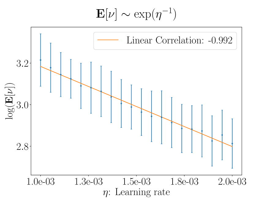
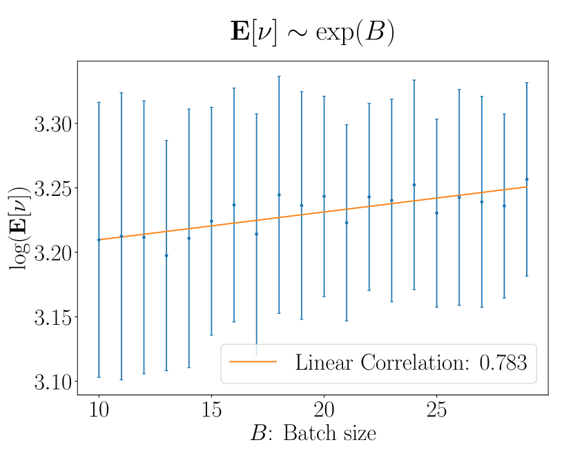
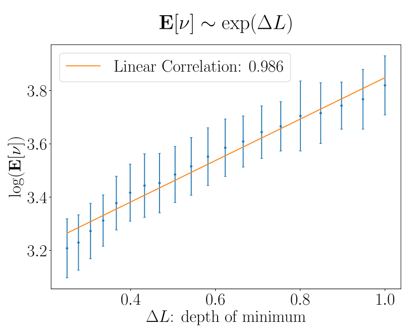
Figure 5: Numerical validation of Theorem 3, where the mean exit time shows exponential dependency on $\lambda_{\mathrm{max}}^{{1}/{2}}$, $\eta^{-1}$, $B$, and $\Delta L$. The error bars indicate the standard deviation.

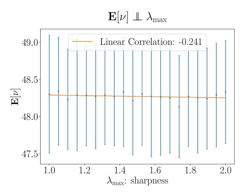
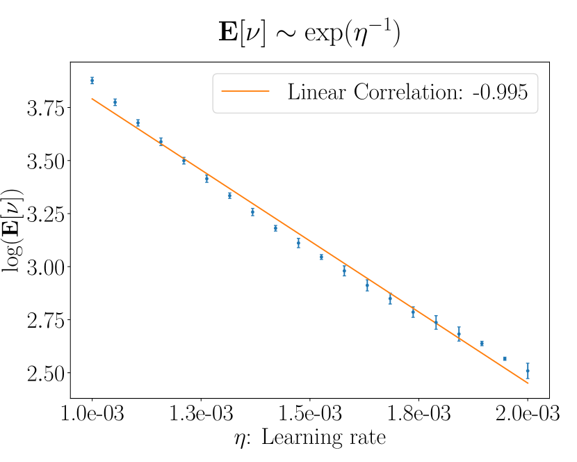
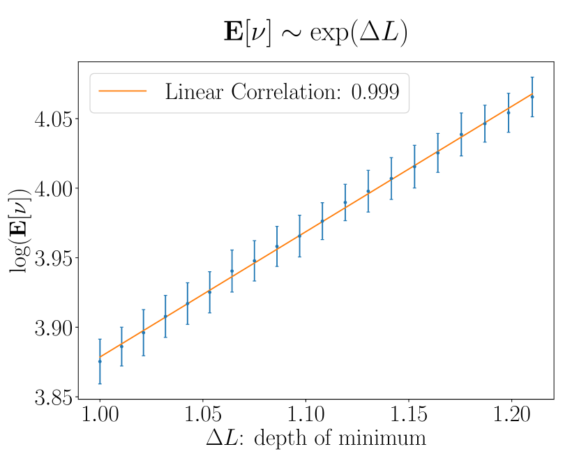
Figure 6: Reference experiment using the proxy system (4). Different from the result of SGD, the exit time has no dependency on $\lambda_{\mathrm{max}}$ while it has exponential dependency on $\eta$ and $\Delta L$ similarly to SGD. This result is aligned with Proposition 1.

6 Comparison with Existing Escape Analyses

We compare our analysis with the closely related existing analyses and discuss the technical differences in detail. As summarized in Table 1 and 2, we picked as closely related analysis, (Hu et al., 2017; Jastrzębski et al., 2017; Zhu et al., 2018; Nguyen et al., 2019; Xie et al., 2020), which analyze how the SGD’s noise affect escape efficiency.

Comparison on exit time

From Table 1, we obtain three implications. (i) In all the results, either or both the learning rate $\eta$ and $H^{*}$ play an important role. (ii) There are four results where the exist time is expressed as an exponential form, and the sharpness-related values $\lambda_{\max}$ and $\bar{\lambda}$ appear in the results of Xie et al. (2020) and our study. (iii) Our study and Xie et al. (2020) have different orders for the parameters for sharpness. This fact will be discussed in the latter half of this section.

Escaping path assumption

We remark that the assumptions of our theorem have an essential difference from Jastrzębski et al. (2017) and Xie et al. (2020). Their analyses assume that SGD escapes along a linear path, named “escape path,” where the gradient perpendicular to the path direction is zero. Escaping path is a convenient assumption to reduce the escape analysis to one-dimensional problems. However, the existence of such paths is supported only weakly by Draxler et al. (2018), and it is unlikely that the stochastic process continuously moves linearly. The fact that we eliminated the escaping path assumptions is a substantial technical improvement.

Effect of sharpness

The technical significance of our theory is that it can analyze the sharpness effect. Because of its non-linearity, sharpness analyses tend to become non-trivial, thus a limited number of existing works have tackled it. Among the selected results, the sharpness effect appears in Jastrzębski et al. (2017) and Zhu et al. (2018) as $H^{*}$, and in Xie et al. (2020) as $\lambda$. We note that the results of Jastrzębski et al. (2017) and Xie et al. (2020) include auxiliary sharpness values, such as $\bar{\lambda}\in[\lambda_{\min},\lambda_{\max}]$ respectively. Those terms appear because of the escaping path assumption and our results show that those terms are not fundamental.

Heavy tailed noise

Among the selected works, only Nguyen et al. (2019) use a heavy-tailed noise model, i.e. the noise whose distribution has a heavier tail than exponential distribution. Although it is known that the heavy-tailed noise models the empirical behavior of SGD well (Simsekli et al., 2019), it is quite difficult to mathematically formulate it. Nguyen et al. (2019) use the Lévy process for their analysis, where $\alpha$ represents the degree of the heavy tail, and $\delta\in(0,1)$ includes miscellaneous constants. Analyzing the sharpness under the heavy-tailed setup is still an open problem.

Study	Exit Time (Order)
Hu et al. (2017)	$\exp(\frac{1}{\eta})$
Jastrzębski et al. (2017)	$\exp\left(\frac{B}{\eta}\Delta L+d\right)$
Zhu et al. (2018)	$\frac{1}{\operatorname{Tr}((H^{*})^{2})}$
Nguyen et al. (2019)	$\frac{1}{{\eta}^{(\alpha-\delta)/2}}$
Xie et al. (2020)	$\exp\left(\frac{B}{\eta}\Delta L\bar{\lambda}^{-1}\right)$
Ours	$\exp\left(\frac{B}{\eta}\left(\Delta L\lambda_{\mathrm{max}}^{-{1}/{2}}\pm\Xi\right)\right)$

Table 1: Results of the derived exit time. We only show their order by ignoring constants. $\Xi=A\lambda_{\mathrm{min}}^{{1}/{2}}(\kappa^{{1}/{2}}-1)$ is the approximation error, $\bar{\lambda}$ is some value in $[\lambda_{\min},\lambda_{\max}]$ defined in Xie et al. (2020), and $\alpha,\delta$ are parameters related to the tail probability (Nguyen et al., 2019).

Studies	Exponential	Sharpness	No	Non-	Discreteness
	escape	analysis	escape paths	stationary
Hu et al. (2017)			$\surd$	$\surd$	$\surd$
Jastrzębski et al. (2017)		$\surd$
Zhu et al. (2018)		$\surd$	$\surd$	$\surd$
Nguyen et al. (2019)			$\surd$	$\surd$	$\surd$
Xie et al. (2020)	$\surd$	$\surd$
Ours	$\surd$	$\surd$	$\surd$	$\surd$	$\surd$

Table 2: Technical difference among analyses. The specific meanings of each column are described in the main passages of Section 6.

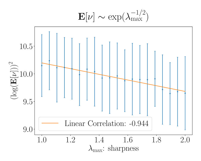
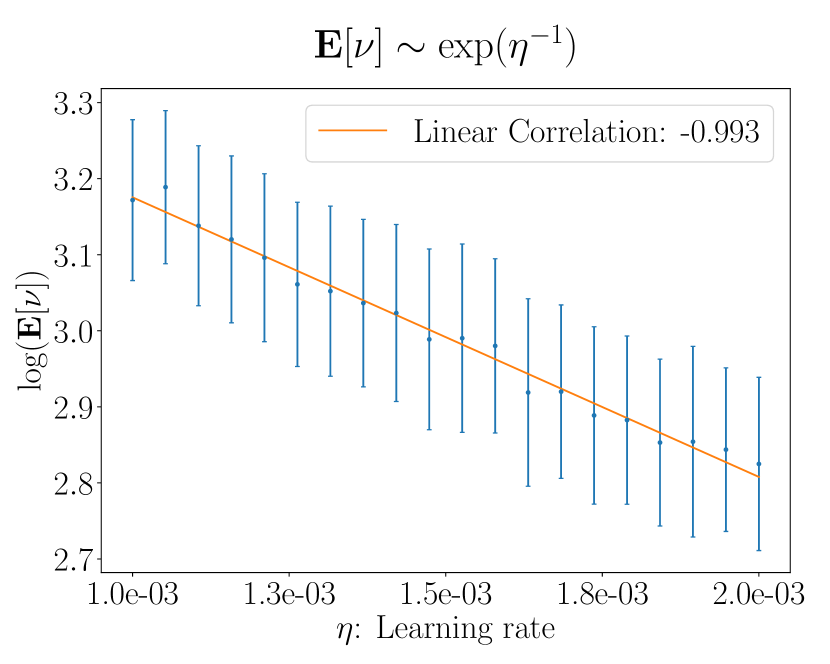
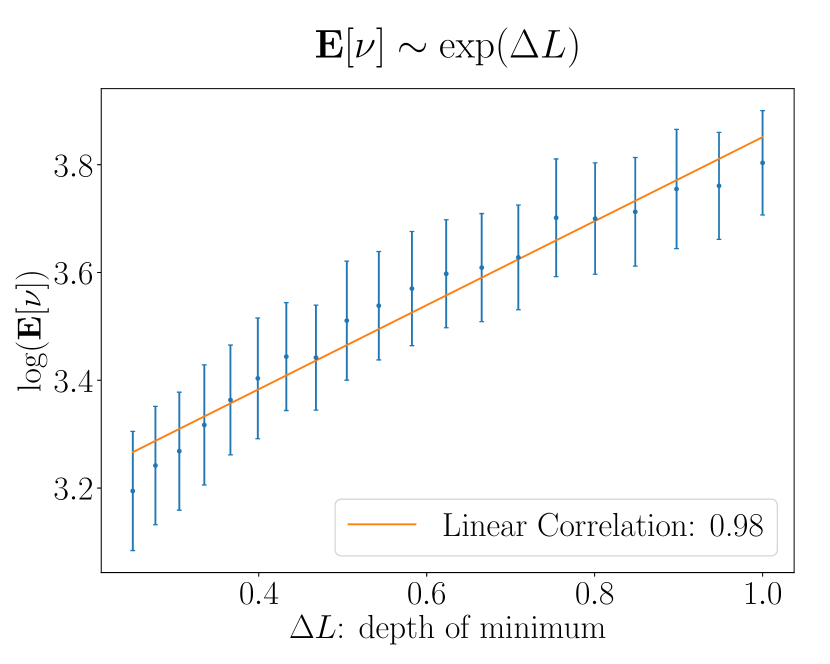
Figure 7: A numerical experiment as in Section 5, but with discrete SGD (2) rather than the original SGD (1). Although they are defined differently, they show similar trends on each parameter. This numerical result shows that (2) is a reasonable model for (1) for exit time analysis.

7 Related Work

Sharpness and generalization of neural networks

The shape of loss surfaces has long been a topic of interest. The argument that the flatness of loss surfaces around local minima improves generalization was first studied by Hochreiter and Schmidhuber (1995, 1997), and the observation has recently been reconfirmed in deep neural networks by Keskar et al. (2016). The theoretical properties of the flatness were criticized by Dinh et al. (2017) in terms of scale-sensitivity of flatness, but there have also been follow-up works tackling the criticism by developing scale-invariant flatness measures (Tsuzuku et al., 2020; Rangamani et al., 2019; Ibayashi et al., 2021). Despite the ongoing theoretical controversy, its empirical benefits seem to be promised (Jiang et al., 2019), thus the training algorithms with sharpness regularizer have achieved state-of-the-art Foret et al. (2020); Kwon et al. (2021). As the other investigations on the loss surface geometry, He et al. (2019b) discussed the asymmetry of loss surfaces, Draxler et al. (2018); Garipov et al. (2018) studied how multiple local minima are internally connected, and Li et al. (2018) developed a random dimensional reduction method to visualize loss surfaces in low dimensions.

SGD and machine learning

The detailed nature of SGD itself is also an object of interest. SGD was first proposed in (Robbins and Monro, 1951), as a lazy version of gradient descent using random subsets of training data. Thus, SGD has been intended to be a convenient heuristic rather than a refined algorithm. However besides its computational convenience, SGD works as effectively as gradient descent does in many optimization problems, and its convergence properties have been solidified on the convex objective functions (Bottou, 2010). The recent success in the field of neural networks is particularly remarkable because it is shown that SGD performs greatly on various non-convex functions as well. In fact, SGD-based training algorithms have been achieving state-of-the-art one after another, e.g., Adagrad (Duchi et al., 2011), Adam (Kingma and Ba, 2014) and many others (Schmidt et al., 2021).

Noise of SGD

Analyzing SGD’s noise has been an appealing topic in the research community. It is known that the magnitude of the gradient noise in SGD has versatile effects on its dynamics Kleinberg et al. (2018) thus it has been closely investigated especially in relation to a learning rate and a batch size. An effect of large batch sizes on the reduction of gradient noise is investigated in Hoffer et al. (2017); Smith et al. (2018); Masters and Luschi (2018). Another area of interest is the shape of a gradient noise distribution. Zhu et al. (2018); Hu et al. (2017); Daneshmand et al. (2018) investigated the anisotropic nature of gradient noise and its advantage. Simsekli et al. (2019) discussed the fact that a gradient noise distribution has a heavier tail than Gaussian distributions. Nguyen et al. (2019); Şimşekli et al. (2019) showed benefits of these heavy tails for SGD. Panigrahi et al. (2019) rigorously examined gradient noise in deep learning and how close it is to a Gaussian. Xie2021-ty studied a situation where the distribution is Gaussian, and then analyzes the behavior of SGD in a theoretical way.

Discretization of SGD

We summarize the approximation we used in Table 4. We used the continuous SGD (3) as an approximation of the discrete SGD (2) because (3) is exactly discretized to (2). This approximation is commonly used because it is well known that the trajectories of those two system show, so-called, “strong convergence” in the order of $O(\sqrt{\eta})$, i.e. $\mathbb{E}(\sup_{0\leq t\leq T}|\theta_{k}^{\mathrm{discrete}}-\theta_{k\eta}|)=O(\eta^{\frac{1}{2}})$ (see e.g. (Gobet, 2016; Cheng et al., 2020)). We note that strong convergence validates the similarity of trajectories, but it does not necessarily guarantee the similarity of escaping behavior. Our work is the first completed argument with Lemma 5 introduced.

As a final remark, (2) is also an approximated model of the original SGD (the dot arrow in Fig. 4). Although this approximation is justified via the central limit theorem (Jastrzębski et al., 2017; He et al., 2019a), it is admittedly heuristic and the quantitative validation for the approximation is assumed to be a (highly non-trivial) open problem. In Fig. 7, we provide empirical results to justify this approximation in our setup for completeness.

8 Conclusion

In this paper, we showed that SGD has exponential escape efficiency from sharp minima even in the non-stationary regime. To reach the goal, we used the Large Deviation Theory and identified that steepness plays the key role in the exponential escape in the non-stationary regime. Our results are the novel theoretical clue to explain the mechanics as to why SGD can find generalizing minima.

Appendix A Stability and Attraction of minima

The followings are the minimum required assumptions for Theorem 1 while both of them are derived from Assumption 1.

Assumption 4 ($\theta^{*}$ is asymptotically stable).

For any neighborhood $U$ that contains $\theta^{*}$, there exists a small neighborhood $V$ of $\theta^{*}$ such that gradient flow with any initial value $\theta_{0}\in V$ does not leave $U$ for $t\geq 0$ and $\lim_{t\rightarrow\infty}\theta_{t}=\theta^{*}$.

Assumption 5 ($D$ is attracted to $\theta^{*}$).

$\forall\theta_{0}\in D$, a system $\dot{\theta}_{t}=-\nabla L(\theta_{t})$ with initial value $\theta_{0}$ converges to $\theta^{*}$ without leaving $D$ as $t\rightarrow\infty$.

Stability is a commonly used notion in dynamical systems [Hu et al., 2017, Wu et al., 2017], although it does not always appear in SGD’s escaping analysis [Zhu et al., 2018, Jastrzębski et al., 2017, Xie et al., 2020]. Assumption 4 is known to be equivalent to the local minimality of $\theta^{*}$ under the condition that $L(\theta)$ is real analytic around $\theta^{*}$ [Absil and Kurdyka, 2006]. Also, by definition of asymptotic stability in Assumption 4, we can always find a region $D$ that satisfies Assumption 5. The more detailed properties of stability can be found, such as in Section 6.5 of Teschl [2000].

Appendix B Proof of Theorem 1

For simplicity, we use $\varepsilon$ to denote $\sqrt{{\eta}/{B}}$. To prove this result, we provide the proof for an upper bound (Lemma 7) and a lower bound (Lemma 8). Throughout the proofs, we use $\mathbf{C}_{T,\theta_{0}}$, $\mathrm{P}_{\theta_{0}}$, instead of $\mathbf{C}_{T}$ or $\mathrm{P}$, to clearly indicate which trajectory we are referring to.

We introduce several notions. For $\delta>0$ and $\theta\in\mathbb{R}^{d}$, let $\mathcal{B}_{\delta}(\theta)$ denote an $\delta$-neighbourhood of $\theta$, that is, $\mathcal{B}_{\delta}(\theta):=\{\theta^{\prime}\in\mathbb{R}^{d}\mid\|\theta^{\prime}-\theta\|\leq\delta\}$. Further, for a set $\Theta\subset\mathbb{R}^{d}$, $\mathcal{B}_{\delta}(\Theta):=\cup_{\theta\in\Theta}\mathcal{B}_{\delta}(\theta)$.

The following lemma provides preliminary facts for proofs.

Lemma 6.

For any $c>0$, there exist $\mu_{1},\mu_{2},T_{1},T_{2}>0$ such that the followings hold:

1. $\forall\theta\in D$, there exists a trajectory $\varphi^{1}$ such that $\varphi_{0}^{1}=\theta$, $\varphi_{T}^{1}\in\mathcal{B}_{\mu_{1}/2}(\theta^{*})$, $0<T\leq T_{1}$ and $S_{T}(\varphi^{1})=0$.

2. $\forall\theta\in\mathcal{B}_{\mu_{1}}(\theta^{*})$, there exists a trajectory $\varphi^{2}$ such that $\varphi^{2}_{0}=\theta$, $\varphi^{2}_{T}\in\partial\mathcal{B}_{\mu_{2}}(D)$, $0<T\leq T_{2}$ and $S_{T}(\varphi^{2})<V_{0}+\frac{c}{2}$.

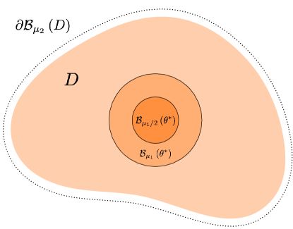
Figure 8: Illustration of domains and boundary, $D$, $\mathcal{B}_{\mu_{1}/2}(\theta^{*})$, $\mathcal{B}_{\mu_{1}}(\theta^{*})$, and $\partial\mathcal{B}_{\mu_{2}}(D)$

The illustration can be found in Fig. 8.

Lemma 6.

The first statement immediately holds by the fact that $D$ is attracted to a asymptotically stable equilibrium position $\theta^{*}$ (Assumption 4 and 5).

For the second statement, since $V_{0}:=\min_{\theta^{\prime}\in\partial D}V\left(\theta^{\prime}\right)$, there exists a trajectory $\varphi^{a}$ such that $\varphi^{a}_{0}=\theta^{*}$, $\varphi^{a}_{T_{a}}\in\partial D$ and $S_{T_{a}}\left(\varphi^{a}\right)=V_{0}$, where $T_{a}$ is finite by Lemma 2.2 (a) in Freidlin and Wentzell [2012]. We cut off the first portion of $\varphi^{a}$ up until the first intersecting point with $\mathcal{B}_{\mu_{1}}(\theta^{*})$ and define it as $\varphi^{b}$. This means $\varphi^{b}_{0}\in\mathcal{B}_{\mu_{1}}(\theta^{*})$, $\varphi^{b}_{T_{b}}\in\partial D$ and $S_{T_{b}}\left(\varphi^{b}\right)<V_{0}$ hold. By Lemma 2.3 in Freidlin and Wentzell [2012], there exists a trajectory from $\varphi^{b}_{T_{b}}$ to a point $\theta_{\mu_{2}}$ in $\partial\mathcal{B}_{\mu_{2}}(D)$ such that the steepness is less than $K|\theta_{\mu_{2}}-\varphi^{b}_{T_{b}}|$ with a constant $K>0$. Then, if we take a small enough $\mu_{2}$, we can obtain $\varphi^{c}$ such $\varphi^{c}_{0}=\varphi^{b}_{T_{b}}$, $\varphi^{c}_{T_{c}}\in\partial\mathcal{B}_{\mu_{2}}(D)$ and $S_{T_{c}}\left(\varphi^{c}\right)<\frac{c}{2}$. By connecting $\varphi^{b}$ and $\varphi^{c}$, we obtain an appropriate $\varphi^{2}$. ∎

Lemma 7.

For any $c>0$, there exists an $\varepsilon_{0}$ such that for $\varepsilon<\varepsilon_{0}$, $\varepsilon^{2}\ln\mathbb{E}\left[\tau\right]<V_{0}+c$ holds, where $V_{0}:=\min_{\theta^{\prime}\in\partial D}V(\theta^{\prime})$.

Proof of Lemma 7.

We split the dynamical system (3) of our interest into the first half and the second half, $\{\theta_{t}^{1}\}_{t}$ and $\{\theta_{t}^{2}\}_{t}$. $\{\theta_{t}^{1}\}_{t}$ starts with $\theta_{0}^{1}=\theta_{0}\in D$ and terminates when it first reaches $\mathcal{B}_{\mu_{1}/2}(\theta^{*})$. We define the terminating time of $\{\theta_{t}^{1}\}_{t}$ as $\tau_{1}:=\min\{t>0:\theta_{t}^{1}\in\mathcal{B}_{\mu_{1}/2}(\theta^{*})\}$. On the other hand, $\{\theta_{t}^{2}\}_{t}$ starts with $\theta_{0}^{2}=\theta_{\tau_{1}}\in\mathcal{B}_{\mu_{1}/2}(\theta^{*})$ and terminates when it first reaches $\partial D$. We define the terminating time of $\{\theta_{t}^{2}\}_{t}$ as $\tau_{2}:=\min\{t>0:\theta_{t}^{1}\in\partial D\}$. Clearly, the exit time $\tau=\tau_{1}+\tau_{2}$.

Regarding $\tau_{1}$ and $\tau_{2}$, we show the following two independent facts with sufficiently small $\varepsilon>0$.

1. : $\tau_{1}$ is no more than $T_{1}$ with probability at least $1/2$.

2. : $\tau_{2}$ is no more than $T_{2}$ with probability at least $\exp\left\{-\varepsilon^{-2}\left(V_{0}+c\right)\right\}$.

Fact 1: Given the trajectory $\varphi_{1}$ provided by Lemma 6, Lemma 1 gives us that if $\varepsilon<\varepsilon_{\mathrm{stp1}}(\varphi_{1},\mu_{1}/2,1)$, the following inequality holds

$$\mathrm{P}_{\theta^{1}_{0}}\Big{\{}\varphi^{\prime}\in\mathbf{C}_{T_{1},\theta_{0}^{1}}(\mathbb{R}^{d})\mid\rho\left(\varphi^{\prime},\varphi_{1}\right)<\mu_{1}/2\Big{\}}\geq\exp\left\{-\varepsilon^{-2}\right\}.$$

Therefore, if we take $\varepsilon<\min\{\sqrt{{1}/{\ln 2}},\varepsilon_{\mathrm{stp1}}(\varphi_{1},\mu_{1}/2,1)\}$, we have

$$\mathrm{P}_{\theta^{1}_{0}}\Big{\{}\varphi^{\prime}\in\mathbf{C}_{T_{1},\theta_{0}^{1}}(\mathbb{R}^{d})\mid\rho\left(\varphi^{\prime},\varphi_{1}\right)<\mu_{1}/2\Big{\}}\geq\frac{1}{2}$$

Since the event of $\{\varphi^{\prime}\in\mathbf{C}_{T_{1},\theta_{0}^{1}}(\mathbb{R}^{d})\mid\rho\left(\varphi^{\prime},\varphi_{1}\right)<\mu_{1}/2\}$ means that $\{\theta_{t}^{1}\}_{t}$ reaches $\mathcal{B}_{\mu_{1}}(\theta^{*})$ in no later than $T_{1}$, we obtain the following which provides Fact 1.

$$\mathrm{P}_{\theta^{1}_{0}}\left\{\tau_{1}<T_{1}\right\}\geq\frac{1}{2}.$$ (7)

Fact 2: Given the trajectory $\varphi_{2}$ provided by Lemma 6, Lemma 1 tells us that if $\varepsilon<\varepsilon_{\mathrm{stp1}}(\varphi_{2},\mu_{2},{c}/{2})$, the following inequality holds

$$\mathrm{P}_{\theta^{2}_{0}}\Big{\{}\varphi^{\prime}\in\mathbf{C}_{T_{2},\theta^{2}_{0}}(\mathbb{R}^{d})\mid\rho\left(\varphi^{\prime},\varphi_{2}\right)<\mu_{2}\Big{\}}\geq\exp\left\{-\varepsilon^{-2}\left(S_{T_{2}}\left(\varphi_{2}\right)+\frac{c}{2}\right)\right\}.$$

$\{\varphi^{\prime}\in\mathbf{C}_{T_{2},\theta^{2}_{0}}(\mathbb{R}^{d})\mid\rho\left(\varphi^{\prime},\varphi_{2}\right)<\mu_{2}\}$ is the event that $\{\theta_{t}^{2}\}_{t}$ goes out of $D$ in no more than the time $T_{2}$. Also, we know that $S_{T_{2}}\left(\varphi_{2}\right)<V_{0}+\frac{c}{2}$ by Lemma 6. Hence, we can conclude the following for Fact 2:

$$\mathrm{P}_{\theta^{2}_{0}}\left\{\tau_{2}<T_{2}\right\} \geq\exp\left\{-\varepsilon^{-2}\left(V_{0}+c\right)\right\}.$$ (8)

Combining (7) and (8), we can obtain

$$\mathrm{P}_{\theta_{0}}\left\{\tau<T_{1}+T_{2}\right\}\geq\frac{1}{2}\exp\left\{-\varepsilon^{-2}\left(V_{0}+c\right)\right\}.$$ (9)

Since this is a simple exponential distribution, we can obtain the following expectation:

$$\mathbb{E}\left[\tau\right]\leq 2\left(T_{1}+T_{2}\right)\exp\left\{\varepsilon^{-2}\left(V_{0}+c\right)\right\}$$

By setting

$$\varepsilon<\frac{1}{\sqrt{\ln 2(T_{1}+T_{2})}}\min\left\{\sqrt{\frac{1}{\ln 2}},\varepsilon_{\mathrm{stp1}}(\varphi_{1},\mu_{1}/2,1),\varepsilon_{\mathrm{stp1}}(\varphi_{2},\mu_{2},{c}/{2})\right\},$$

we can get

$$\mathbb{E}\left[\tau\right]\leq\exp\left\{\varepsilon^{-2}\left(V_{0}+c\right)\right\}.$$

Then, we obtain the statement. ∎

Next, we develop the lower bound on the exit time.

Lemma 8.

For any $c>0$, there exists an $\varepsilon_{0}$ such that for $\varepsilon<\varepsilon_{0}$, $\varepsilon^{2}\ln\mathbb{E}\left[\tau\right]>V_{0}-c$ holds, where $V_{0}:=\min_{\theta^{\prime}\in\partial D}V(\theta^{\prime})$.

Lemma 8.

We consider a specific case where the initial value of (3) is in $\partial\mathcal{B}_{\mu_{1}/2}(\theta^{*})$, which can be trivially extended to general cases. Consider a Markov chain $Z_{k}\;(k\in\mathbb{N})$ as a discretization of $\theta_{t}$ as $t=\tau_{k}$ with a $k$-th time grid $\tau_{k}$. It is formally defined as follows:

1. $\tau_{0}=0$,

2. $\sigma_{k}=\inf\left\{t>\tau_{k}\right.\text{ : }\left.\theta_{t}\in\partial\mathcal{B}_{\mu_{1}}(\theta^{*})\right\}$,

3. $\tau_{k}=\inf\left\{t>\sigma_{k-1}:\theta_{t}\in\partial\mathcal{B}_{\mu_{1}/2}(\theta^{*})\cup\partial D\right\}$,

4. $Z_{k}=\theta_{\tau_{k}}$.

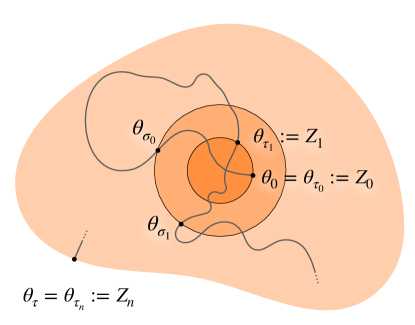
Figure 9: A continuous trajectory $\theta_{t}$ and the Markov chain $Z_{k}$ generated from $\{\theta_{t}\}_{t}$. Colored domains indicate $D$, $\mathcal{B}_{\mu_{1}/2}(\theta^{*})$, and $\mathcal{B}_{\mu_{1}}(\theta^{*})$ as illustrated in Fig. 8.

By introducing $Z_{k}$, we can reduce the continuous process $\{\theta_{t}\}_{t}$ to a discrete Markov chain transiting between $\partial\mathcal{B}_{\mu_{1}/2}\left(\theta^{*}\right)$ and $\partial D$. The illustration can be found in Fig. 9.

Let $\kappa:=\inf\{k\mid Z_{k}\in\partial D\}$. Then, we have $\tau=\tau_{n}$ and

$$\mathbb{E}\left[\tau\right] =\sum_{k=0}^{\infty}\Big{(}\mathrm{P}_{\theta_{0}}\left\{\kappa\geq k\right\}-\mathrm{P}_{\theta_{0}}\left\{\kappa\geq k+1\right\}\Big{)}\tau_{k}=\sum_{k=1}^{\infty}\mathrm{P}_{\theta_{0}}\left\{\kappa\geq n\right\}\left(\tau_{k}-\tau_{k-1}\right).$$

This can be further evaluated as

$$\mathbb{E}\left[\tau\right] >\sum_{k=1}^{\infty}\mathrm{P}_{\theta_{0}}\left\{\kappa\geq k\right\}\left(\tau_{k}-\sigma_{k-1}\right)>\sum_{k=1}^{\infty}\mathrm{P}_{\theta_{0}}\left\{\kappa\geq n\right\}\Big{(}\inf_{\theta_{0}\in\partial\mathcal{B}_{\mu_{1}}(\theta^{*})}\mathbb{E}[\tau_{1}]\Big{)},$$

which follows $\tau_{k-1}<\sigma_{k-1}$. Since $\mathcal{B}_{\mu_{1}/2}(\theta^{*})$ is a strict subset of $\mathcal{B}_{\mu_{1}}(\theta^{*})$, and $\mathcal{B}_{\mu_{1}}(\theta^{*})$ is a strict subset of $D$, it takes a positive amount of time to transit from $\partial\mathcal{B}_{\mu_{1}}(\theta^{*})$ to either $\partial\mathcal{B}_{\mu_{1}/2}(\theta^{*})$ or $\partial D$, and there exists a positive lower bound $t_{1}$ for $\inf_{\theta_{0}\in\mathcal{B}_{\mu_{1}}(\theta^{*})}\mathbb{E}[\tau_{1}]$ that is independent of $\varepsilon$. Thus we get

$$\mathbb{E}\left[\tau\right]>t_{1}\sum_{k=1}^{\infty}\mathrm{P}_{\theta_{0}}\left\{\kappa\geq k\right\}.$$

By Lemma 9, we immediately get $\mathrm{P}_{\theta_{0}}\{\kappa>k\}\geq[1-\exp\{-\varepsilon^{-2}(V_{0}-c)\}]^{k-1}$, hence we have

$$\mathbb{E}\left[\tau\right] >t_{1}\sum_{k=1}^{\infty}\left[1-\exp\left\{-\varepsilon^{-2}\left(V_{0}-c\right)\right\}\right]^{k-1}=t_{1}\exp\left\{\varepsilon^{-2}\left(V_{0}-c\right)\right\}.$$

This implies $\mathbb{E}[\tau]\geq\exp\{\varepsilon^{-2}(V_{0}-c)\}$ holds if $\varepsilon$ is small enough. ∎

Lemma 9.

We obtain

$$\mathrm{P}(Z_{k+1}\in\partial D\mid Z_{k}\in\mathcal{B}_{\mu_{1}/2}(\theta^{*}))\leq\exp\left\{-\varepsilon^{-2}\left(V_{0}-c\right)\right\}.$$

Lemma 9.

First, we decompose $\mathrm{P}(Z_{k+1}\in\partial D\mid Z_{k}\in\partial\mathcal{B}_{\mu_{1}/2}(\theta^{*}))$ into two parts in the following way:

$$\begin{aligned} &\mathrm{P}_{\theta_{0}}(Z_{k+1}\in\partial D\mid Z_{k}\in\partial\mathcal{B}_{\mu_{1}/2}(\theta^{*}))\\ &\leq\max_{\theta^{\prime}_{0}\in\partial\mathcal{B}_{\mu_{1}/2}(\theta^{*})}P_{\theta^{\prime}_{0}}\left\{\tau_{1}=\tau\right\}\\ &=\max_{\theta^{\prime}_{0}\in\partial\mathcal{B}_{\mu_{1}/2}(\theta^{*})}\Big{[}\mathrm{P}_{\theta^{\prime}_{0}}\left\{\tau=\tau_{1}<T\right\}+\mathrm{P}_{\theta^{\prime}_{0}}\left\{\tau=\tau_{1}\geq T\right\}\Big{]}\end{aligned}$$ (10)

This holds for arbitrary $T$, so we pick $T=T^{\prime}$ large enough so that this inequality holds for the first term:

$$\mathrm{P}_{\theta^{\prime}_{0}}\left\{\tau=\tau_{1}\geq T^{\prime}\right\}\leq\frac{1}{2}\exp\left\{-\varepsilon^{-2}\left(V_{0}-c\right)\right\}$$ (11)

The existence of such $T^{\prime}$ is guaranteed by the fact that $V_{0}$ is finite and the following lemma.

Lemma 10 (Lemma 2.2 (b) in Freidlin and Wentzell [2012]).

For any $\alpha>0$, there exists positive constants $c$ and $T_{0}$, such that for all sufficiently small $\varepsilon>0$ and any $\theta_{0}\in D\cup\partial D\backslash\mathcal{B}_{\alpha}(\theta^{*})$ we have the inequality

$$\mathrm{P}_{\theta_{0}}\left\{\zeta_{\alpha}>T\right\}\leq\exp\left\{-\varepsilon^{-2}c\left(T-T_{0}\right)\right\},$$

where $\zeta_{\alpha}=\inf\left\{t:\theta_{t}\notin D\backslash\mathcal{B}_{\alpha}(\theta^{*})\right\}$.

Given a constant $T^{\prime}$, we consider bounding $\mathrm{P}_{\theta^{\prime}_{0}}\left\{\tau=\tau_{1}<T^{\prime}\right\}$. Consider the following set of trajectories:

$$\Phi(V_{0}-c/2):=\{\varphi:\varphi_{0}=\theta^{\prime}_{0},S_{T}(\varphi)\leq V_{0}-c/2\}.$$

Since it takes at least $V_{0}$ to reach $\partial D$ from $\theta^{*}$, the following inequality holds:

$$\mathrm{P}_{\theta^{\prime}_{0}}\left\{\tau=\tau_{1}<T^{\prime}\right\} \leq\mathrm{P}_{\theta^{\prime}_{0}}\left\{\varphi_{y}\notin\Phi(V_{0}-c/2)\right\}.$$

Also, Lemma 2 implies, for all $\varepsilon\leq\varepsilon_{\mathrm{stp2}}(V_{0}-c/2,\delta,c/2)$

$$\mathrm{P}_{\varphi^{\prime}}\Big{\{}\varphi^{\prime}\in\mathbf{C}_{T,\theta^{\prime}_{0}}(\mathbb{R}^{d})\mid\rho\big{(}(\varphi^{\prime}-\Phi(V_{0}-c/2)\big{)}\geq\delta\Big{\}} \leq\exp\{-\varepsilon^{-2}((V_{0}-c/2)-c/2)\}$$

$$=\exp\{-\varepsilon^{-2}(V_{0}-c)\}$$

Since $\delta$ can be arbitrarily small, the event of $\{\varphi_{y}\notin\Phi(V_{0}-c/2)\}$ is equal to the event of $\{\varphi^{\prime}\in\mathbf{C}_{T,\theta^{\prime}_{0}}(\mathbb{R}^{d})\mid\rho((\varphi^{\prime}-\Phi(V_{0}-c/2))\geq\delta\}$. Hence, we obtain

$$\mathrm{P}_{\theta^{\prime}_{0}}\left\{\tau=\tau_{1}<T\right\}<\exp\{-\varepsilon^{-2}(V_{0}-c)\}.$$ (12)

If we set $\varepsilon\leq\frac{1}{\sqrt{\ln 2}}\varepsilon_{\mathrm{stp2}}(V_{0}-c/2,\delta,c/2)$, we conclude

$$\mathrm{P}_{\theta^{\prime}_{0}}\left\{\tau=\tau_{1}<T\right\}<\frac{1}{2}\exp\{-\varepsilon^{-2}(V_{0}-c)\}.$$ (13)

Combining (10), (11), and (13), we prove the statement. ∎

Appendix C Hamilton-Jacobi Equation for Quasi-potential

While we use a proximal system to approximate the quasi-potential, there have been attempts to directly analyze $V(\theta)$. A prominent result is the theorem by Hu et al. [2019], which showed that $V(\theta)$ satisfies the following Hamilton–Jacobi equation.

Theorem 4.

For all $\theta\in D$, $V(\theta)$ satisfies the following Jacobi equation,

$$\frac{1}{2}\nabla V(\theta)^{\top}{C\left(\theta\right)}^{1/2}\nabla V(\theta)-\nabla L\left(\theta\right)^{\top}\nabla V(\theta)=0$$

Although it does not give us a closed solution of $V(\theta)$, it reflects the role of $C(\theta)$ to make $V(\theta)$ smaller. Below, we provide the proof in our notation for the completeness.

Proof.

For $u,v\in\mathbb{R}^{d}$, we introduce an inner product and a norm regarding a point $\theta\in D$ as $\langle u,v\rangle_{\theta}:=u^{\top}C\left(\theta\right)^{-1/2}v$ and $\|u\|_{\theta}:=\sqrt{\langle u,u\rangle_{\theta}}$. With these definitions, the $S_{T}(\varphi)$ is written as follows:

$$S_{T}(\varphi)=\frac{1}{2}\int_{0}^{T}\left\|\dot{\varphi}_{t}+\nabla L\left(\varphi_{t}\right)\right\|_{\varphi_{t}}^{2}dt.$$ (14)

Note that $\varphi_{t}\in D$ holds for any $t\in[0,T]$ by the definition of trajectories. We rewrite the integrand of (14) as follows:

$$\left\|\dot{\varphi}_{t}+\nabla L\left(\varphi_{t}\right)\right\|_{\varphi_{t}}^{2}$$

$$=\left\|\dot{\varphi}_{t}\right\|_{\varphi_{t}}^{2}+\left\|\nabla L\left(\varphi_{t}\right)\right\|_{\varphi_{t}}^{2}+2\left\langle\dot{\varphi}_{t},\nabla L\left(\varphi_{t}\right)\right\rangle_{\varphi_{t}}$$

$$=\left(\left\|\dot{\varphi}_{t}\right\|_{\varphi_{t}}-\left\|\nabla L\left(\varphi_{t}\right)\right\|_{\varphi_{t}}\right)^{2}+2\left\|\dot{\varphi}_{t}\right\|_{\varphi_{t}}\left\|\nabla L\left(\varphi_{t}\right)\right\|_{\varphi_{t}}+2\left\langle\dot{\varphi}_{t},\nabla L\left(\varphi_{t}\right)\right\rangle_{\varphi_{t}}$$

$$\geq 2\left\|\dot{\varphi}_{t}\right\|_{\varphi_{t}}\left\|\nabla L\left(\varphi_{t}\right)\right\|_{\varphi_{t}}+2\left\langle\dot{\varphi}_{t},\nabla L\left(\varphi_{t}\right)\right\rangle_{\varphi_{t}}.$$ (15)

We develop a parameterization for the term in (15). For a trajectory $\varphi$, we select an bijective function $f:[0,1]\to[0,T]$ as satisfying the follows: for each $t\in[0,T]$ and $t^{*}\in[0,1]$ as $t=f(t^{*})$, a parameterized trajectory $\varphi^{*}_{t^{*}}:=\varphi_{f(t^{*})}$ satisfies

$$\left\|\dot{\varphi}^{*}_{t^{*}}\right\|_{\varphi^{*}_{t^{*}}}=\|\nabla L(\dot{\varphi}^{*}_{t^{*}})\|_{\varphi^{*}_{t^{*}}}.$$ (16)

This parameterization reduces the quasi-potential to the minimum of the following quantity:

$$(S_{T}(\varphi)\geq S_{f(T)}(\varphi^{*})=)\int^{f(T)}_{0}\left\|\dot{\varphi}^{*}_{t^{*}}\right\|_{\varphi^{*}_{t^{*}}}\left\|\nabla L\left(\varphi^{*}_{t^{*}}\right)\right\|_{\varphi^{*}_{t^{*}}}+\left\langle\dot{\varphi}^{*}_{t^{*}},\nabla L\left(\varphi^{*}_{t^{*}}\right)\right\rangle_{\varphi^{*}_{t^{*}}}dt^{*}$$ (17)

subject to the constraint (16). Since the integrand of (17) includes the first order derivative regarding $t^{*}$, (17) holds over different parameterizations $f$. For convenience, we use another bijective parameterization function $g:[0,R]\to[0,1]$ as $t^{*}=g(r)$ with $R>0$ and $r\in[0,R]$ such that $\hat{\varphi}_{r}:=\varphi^{*}_{g(r)}$ satisfies

$$\|\dot{\hat{\varphi}}_{r}\|_{\hat{\varphi}_{r}}=1.$$ (18)

Then, the quasi-potential is reduced to the following formula,

$$V(\theta)=\inf_{r\in[0,R]:\|\dot{\hat{\varphi}}_{r}\|_{\hat{\varphi}_{r}}=1}\int^{R}_{0}\left(\|\dot{\hat{\varphi}}_{r}\|_{\hat{\varphi}_{r}}\left\|\nabla L\left(\hat{\varphi}_{r}\right)\right\|_{\hat{\varphi}_{r}}+\left\langle\dot{\hat{\varphi}}_{r},\nabla L\left(\hat{\varphi}_{r}\right)\right\rangle_{\hat{\varphi}_{r}}\right)dr,$$ (19)

where $\hat{\varphi}_{R}=\theta$. By the Bellman equation-type optimality, we expand the right hand side of (19) into the following form:

$$V(\theta)=\inf_{r\in[0,R]:\|\dot{\hat{\varphi}}_{r}\|_{\hat{\varphi}_{r}}=1}\left(\int^{R}_{R-\delta}\left(\|\dot{\hat{\varphi}}_{r}\|_{\hat{\varphi}_{r}}\left\|\nabla L\left(\hat{\varphi}_{r}\right)\right\|_{\hat{\varphi}_{r}}+\left\langle\dot{\hat{\varphi}}_{r},\nabla L\left(\hat{\varphi}_{r}\right)\right\rangle_{\hat{\varphi}_{r}}\right)dr+V(\hat{\varphi}_{R-\delta})\right),$$ (20)

with a width value $\delta>0$. The Taylor expansion around $r=R$ gives

$$\int^{R}_{R-\delta}\left(\|\dot{\hat{\varphi}}_{r}\|_{\hat{\varphi}_{r}}\left\|\nabla L\left(\hat{\varphi}_{r}\right)\right\|_{\hat{\varphi}_{r}}+\left\langle\dot{\hat{\varphi}}_{r},\nabla L\left(\hat{\varphi}_{r}\right)\right\rangle_{\hat{\varphi}_{r}}\right)dr+V(\hat{\varphi}_{R-\delta})$$

$$=\delta\left(\|\nabla L(\hat{\varphi}_{R})\|_{\hat{\varphi}_{R}}+\left\langle\nabla L(\hat{\varphi}_{R}),\dot{\hat{\varphi}}_{R}\right\rangle_{\hat{\varphi}_{R}}-\dot{\hat{\varphi}}_{R}^{\top}\nabla V\left(\hat{\varphi}_{R}\right)\right)+V\left(\hat{\varphi}_{R}\right)+O\left(\delta^{2}\right)$$

Taking $\delta\to 0$ and noticing $\hat{\varphi}_{R}=\theta$, (20) can be simplified to the following equation:

$$0=\inf_{r\in[0,R]:\|\dot{\hat{\varphi}}_{r}\|_{\hat{\varphi}_{r}}=1}\left(\|\nabla L(\theta)\|_{\theta}+\left\langle\nabla L(x)^{\top},\dot{\hat{\varphi}}_{R}\right\rangle_{\theta}-\dot{\hat{\varphi}}_{R}\nabla V\left(\theta\right)\right)$$ (21)

It remains to select $\hat{\varphi}$ which solves the minimization problem (21). Since the following equality holds,

$$\left\langle\nabla L(\theta)^{\top},\dot{\hat{\varphi}}_{R}\right\rangle_{\theta}-\dot{\hat{\varphi}}_{R}\nabla V\left(\theta\right)=\left\langle\nabla L(\theta)^{\top}-\nabla V\left(\theta\right)^{\top}C\left(\theta\right)^{-1/2},\dot{\hat{\varphi}}_{R}\right\rangle_{\theta},$$ (22)

it is easy to see that a trajectory $\hat{\varphi}^{*}$ such that

$$\dot{\hat{\varphi}}^{*}_{R}=-\frac{\nabla L(x)^{\top}-\nabla V\left(\theta\right)C\left(\theta\right)^{1/2}}{\|\nabla L(\theta)^{\top}-\nabla V\left(\theta\right)C\left(\theta\right)^{1/2}\|_{\theta}}$$

minimizes (22). With this $\hat{\varphi}^{*}$, (21) simplifies to

$$\|\nabla L(\theta)\|_{\theta}=\|\nabla L(\theta)^{\top}-\nabla V\left(\theta\right)C\left(\theta\right)^{1/2}\|_{\theta}.$$

Taking the square of both sides, we get the statement. ∎

Appendix D Proof of Lemma 4

Proof.

First, we use $\lambda_{\mathrm{max}}^{-\frac{1}{2}}\hat{S}_{T}(\varphi)$ as a “proxy steepness” to estimate $S(\varphi)$ and $V(\theta)$. For any trajectory $\varphi$, the following bound holds.

$$\left|S_{T}(\varphi)-\lambda_{\mathrm{max}}^{-\frac{1}{2}}\hat{S}_{T}(\varphi)\right|$$ (23)

$$=\left|\frac{1}{2}\int_{0}^{T}\left(\dot{\varphi}_{t}+\nabla L\left(\varphi_{t}\right)\right)^{\top}C\left(\varphi_{t}\right)^{-1/2}\left(\dot{\varphi}_{t}+\nabla L\left(\varphi_{t}\right)\right)dt-\frac{1}{2}\lambda_{\mathrm{max}}^{-\frac{1}{2}}\int_{0}^{T}\left\|\dot{\varphi}_{t}+\nabla L\left(\varphi_{t}\right)\right\|^{2}dt\right|$$ (24)

$$=\left|\frac{1}{2}\int_{0}^{T}\left(\dot{\varphi}_{t}+\nabla L\left(\varphi_{t}\right)\right)^{\top}\left(C\left(\varphi_{t}\right)^{-1/2}-\lambda_{\mathrm{max}}^{-\frac{1}{2}}I\right)\left(\dot{\varphi}_{t}+\nabla L\left(\varphi_{t}\right)\right)dt\right|$$ (25)

$$\leq\frac{1}{2}\int_{0}^{T}\left|\left(\dot{\varphi}_{t}+\nabla L\left(\varphi_{t}\right)\right)^{\top}\left(C\left(\varphi_{t}\right)^{-1/2}-\lambda_{\mathrm{max}}^{-\frac{1}{2}}I\right)\left(\dot{\varphi}_{t}+\nabla L\left(\varphi_{t}\right)\right)\right|dt$$ (26)

Since $C\left(\varphi_{t}\right)^{-1/2}-\lambda_{\mathrm{max}}^{-\frac{1}{2}}I$ is positive semi-definite,

$$(\ref{eq:steepness_upperbound}) \leq\frac{1}{2}\int_{0}^{T}\left\|\dot{\varphi}_{t}+\nabla L\left(\varphi_{t}\right)\right\|^{2}\lambda_{\mathrm{max}}\left(C\left(\varphi_{t}\right)^{-1/2}-\lambda_{\mathrm{max}}^{-\frac{1}{2}}I\right)dt$$ (27)

Since $D$ is a finite set and $L(\theta)$ is a locally quadratic funciton (Assumption 1), there exists a constant $M>0$ that satisfies $\forall\theta\in D:\|\nabla L(\theta)\|\leq M$. Combined with Assumption 2 and 3, we can further obtain the following bound.

$$(\ref{eq:steepness_upperbound_psd}) \leq\frac{T}{2}(K+M)^{2}\sup_{0\leq t\leq T}\left\{\lambda_{\mathrm{max}}\left(C\left(\varphi_{t}\right)^{-1/2}-\lambda_{\mathrm{max}}^{-\frac{1}{2}}I\right)\right\}$$ (28)

$$\quad(\because\|\nabla L(\theta)\|\leq M\textrm{ and Assumption \ref{assumption:trajectory_grad_bound}})$$

$$=\frac{T}{2}(K+M)^{2}\sup_{0\leq t\leq T}\left\{\lambda_{\mathrm{max}}\left(C\left(\varphi_{t}\right)^{-1/2}\right)-\lambda_{\mathrm{max}}^{-\frac{1}{2}}\right\}$$ (29)

$$\leq\frac{T}{2}(K+M)^{2}\left(\lambda_{\mathrm{min}}^{-\frac{1}{2}}-\lambda_{\mathrm{max}}^{-\frac{1}{2}}\right)\quad(\because\textrm{Assumption \ref{assumption:strong_covariance}})$$ (30)

With this upper bound, $V_{0}$ can also be bounded in the followings. By definition,

$$V_{0} =\inf_{\theta\in\partial D}\inf_{T>0}\inf_{\varphi:\begin{subarray}{c}(\varphi_{0},\varphi_{T})=(\theta^{*},\theta)\end{subarray}}S_{T}(\varphi)$$ (31)

$$\hat{V}_{0} =\inf_{\theta\in\partial D}\inf_{T>0}\inf_{\varphi:\begin{subarray}{c}(\varphi_{0},\varphi_{T})=(\theta^{*},\theta)\end{subarray}}\hat{S}_{T}(\varphi)$$ (32)

From here below, we denote $\inf_{\varphi:\begin{subarray}{c}(\varphi_{0},\varphi_{T})=(\theta^{*},\theta)\end{subarray}}$ by $\inf_{\varphi(\theta,T)}$ for brevity.

Since $\partial D$ is a continuous finite boundary, we have the following $\theta^{\dagger}$ and $\theta^{*}$.

$$\theta^{\dagger}:=\underset{\theta\in\partial D}{\arg\!\inf}\inf_{T>0}\inf_{\varphi(\theta,T)}S_{T}(\varphi)$$ (33)

$$\theta^{*}:=\underset{\theta\in\partial D}{\arg\!\inf}\inf_{T>0}\inf_{\varphi(\theta,T)}\hat{S}_{T}(\varphi).$$ (34)

The followings hold.

$$\inf_{\theta\in\partial D}\inf_{T>0}\inf_{\varphi(\theta,T)}S_{T}(\varphi)-\inf_{\theta\in\partial D}\inf_{T>0}\inf_{\varphi(\theta,T)}\hat{S}_{T}(\varphi)\leq\inf_{T>0}\inf_{\varphi(\theta^{*},T)}S_{T}(\varphi)-\inf_{T>0}\inf_{\varphi(\theta^{*},T)}\hat{S}_{T}(\varphi)$$ (35)

$$\inf_{\theta\in\partial D}\inf_{T>0}\inf_{\varphi(\theta,T)}\hat{S}(\varphi)-\inf_{\theta\in\partial D}\inf_{T>0}\inf_{\varphi(\theta,T)}S_{T}(\varphi)\leq\inf_{T>0}\inf_{\varphi(\theta^{\dagger},T)}\hat{S}_{T}(\varphi)-\inf_{T>0}\inf_{\varphi(\theta^{\dagger},T)}S_{T}(\varphi)$$ (36)

Similarly, we can restrict our focus on finite $T$ in the exit time analysis (Lemma 6). Thus, for each $\theta$, we have the following finite $T^{\dagger}$ and $T^{*}$.

$$T^{\dagger}(\theta):=\underset{T>0}{\arg\!\inf}\inf_{\varphi(\theta,T)}S_{T}(\varphi)$$ (37)

$$T^{*}(\theta):=\underset{T>0}{\arg\!\inf}\inf_{\varphi(\theta,T)}\hat{S}_{T}(\varphi),$$ (38)

and the followings hold

$$\inf_{T>0}\inf_{\varphi(\theta^{*},T)}S_{T}(\varphi)-\inf_{T>0}\inf_{\varphi(\theta^{*},T)}\hat{S}_{T}(\varphi)\leq\inf_{\varphi(\theta^{*},T^{*}(\theta^{*}))}S_{T^{*}(\theta^{*})}(\varphi)-\inf_{\varphi(\theta^{*},T^{*}(\theta^{*}))}\hat{S}_{T^{*}(\theta^{*})}(\varphi)$$ (39)

$$\inf_{T>0}\inf_{\varphi(\theta^{\dagger},T)}\hat{S}_{T}(\varphi)-\inf_{T>0}\inf_{\varphi(\theta^{\dagger},T)}S_{T}(\varphi)\leq\inf_{\varphi(\theta^{\dagger},T^{\dagger}(\theta^{\dagger}))}\hat{S}_{T^{\dagger}(\theta^{\dagger})}(\varphi)-\inf_{\varphi(\theta^{\dagger},T^{\dagger}(\theta^{\dagger}))}S_{T^{\dagger}(\theta^{\dagger})}(\varphi).$$ (40)

Similarly, since $L(\theta)$ and $C(\theta)$ are continuous, for each $\theta$ and $T$, we have the followings

$$\varphi^{\dagger}(\theta,T):=\underset{\varphi(\theta,T)}{\arg\!\inf}S_{T}(\varphi)$$ (41)

$$\varphi^{*}(\theta,T):=\underset{\varphi(\theta,T)}{\arg\!\inf}\hat{S}_{T}(\varphi).$$ (42)

and we get

$$\inf_{\varphi(\theta^{*},T^{*}(\theta^{*}))}S_{T^{*}(\theta^{*})}(\varphi)-\inf_{\varphi(\theta^{*},T^{*}(\theta^{*}))}\hat{S}_{T^{*}}(\varphi) \leq S_{T^{*}(\theta^{*})}(\varphi^{*}(\theta^{*},T^{*}(\theta^{*})))-\hat{S}_{T^{*}}(\varphi^{*}(\theta^{*},T^{*}(\theta^{*})))$$ (43)

$$\leq\frac{T^{*}(\theta^{*})}{2}(K+M)^{2}\left(\lambda_{\mathrm{min}}^{-\frac{1}{2}}-\lambda_{\mathrm{max}}^{-\frac{1}{2}}\right)$$ (44)

$$\inf_{\varphi(\theta^{\dagger},T^{\dagger}(\theta^{\dagger}))}\hat{S}_{T^{\dagger}(\theta^{\dagger})}(\varphi)-\inf_{\varphi(\theta^{\dagger},T^{\dagger}(\theta^{\dagger}))}S_{T^{\dagger}(\theta^{\dagger})}(\varphi) \leq\hat{S}_{T^{\dagger}(\theta^{\dagger})}(\varphi^{\dagger}(\theta^{\dagger},T^{\dagger}(\theta^{\dagger})))-S_{T^{\dagger}(\theta^{\dagger})}(\varphi^{\dagger}(\theta^{\dagger},T^{\dagger}(\theta^{\dagger})))$$ (45)

$$\leq\frac{T^{\dagger}(\theta^{\dagger})}{2}(K+M)^{2}\left(\lambda_{\mathrm{min}}^{-\frac{1}{2}}-\lambda_{\mathrm{max}}^{-\frac{1}{2}}\right)$$ (46)

Thus we get

$$\left|V_{0}-\lambda^{-\frac{1}{2}}\hat{V}_{0}\right|\leq\frac{\max\{T^{\dagger}(\theta^{\dagger}),T^{*}(\theta^{*})\}}{2}(K+M)^{2}\left(\lambda_{\mathrm{min}}^{-\frac{1}{2}}-\lambda_{\mathrm{max}}^{-\frac{1}{2}}\right)$$ (47)

Defining $A:=\frac{\max\{T^{\dagger}(\theta^{\dagger}),T^{*}(\theta^{*})\}}{2}(K+M)^{2}$ finishes the proof.

∎

References

- Li et al. [2018] Hao Li, Zheng Xu, Gavin Taylor, Christoph Studer, and Tom Goldstein. Visualizing the loss landscape of neural nets. Advances in Neural Information Processing Systems, 31, 2018.
- Blum and Rivest [1992] Avrim L Blum and Ronald L Rivest. Training a 3-node neural network is np-complete. Neural Networks, 5(1):117–127, 1992.
- Zhang et al. [2017] Chiyuan Zhang, Samy Bengio, Moritz Hardt, Benjamin Recht, and Oriol Vinyals. Understanding deep learning requires rethinking generalization (2016). arXiv preprint arXiv:1611.03530, 2017.
- Keskar et al. [2016] Nitish Shirish Keskar, Dheevatsa Mudigere, Jorge Nocedal, Mikhail Smelyanskiy, and Ping Tak Peter Tang. On large-batch training for deep learning: Generalization gap and sharp minima. arXiv preprint arXiv:1609.04836, 2016.
- Dziugaite and Roy [2017] Gintare Karolina Dziugaite and Daniel M Roy. Computing nonvacuous generalization bounds for deep (stochastic) neural networks with many more parameters than training data. arXiv preprint arXiv:1703.11008, 2017.
- Jiang et al. [2019] Yiding Jiang, Behnam Neyshabur, Hossein Mobahi, Dilip Krishnan, and Samy Bengio. Fantastic generalization measures and where to find them. arXiv preprint arXiv:1912.02178, 2019.
- Zhu et al. [2018] Zhanxing Zhu, Jingfeng Wu, Bing Yu, Lei Wu, and Jinwen Ma. The anisotropic noise in stochastic gradient descent: Its behavior of escaping from sharp minima and regularization effects. arXiv preprint arXiv:1803.00195, 2018.
- Xie et al. [2020] Zeke Xie, Issei Sato, and Masashi Sugiyama. A diffusion theory for deep learning dynamics: Stochastic gradient descent exponentially favors flat minima. In International Conference on Learning Representations, 2020.
- Simonyan and Zisserman [2014] Karen Simonyan and Andrew Zisserman. Very deep convolutional networks for large-scale image recognition. arXiv preprint arXiv:1409.1556, 2014.
- Krizhevsky et al. [2009] Alex Krizhevsky, Geoffrey Hinton, et al. Learning multiple layers of features from tiny images. 2009.
- Jastrzębski et al. [2017] Stanisław Jastrzębski, Zachary Kenton, Devansh Arpit, Nicolas Ballas, Asja Fischer, Yoshua Bengio, and Amos Storkey. Three factors influencing minima in sgd. arXiv preprint arXiv:1711.04623, 2017.
- Kramers [1940] H A Kramers. Brownian motion in a field of force and the diffusion model of chemical reactions. Physica, 7(4):284–304, April 1940.
- Eyring [1935] Henry Eyring. The activated complex in chemical reactions. The Journal of Chemical Physics, 3(2):107–115, 1935.
- Hanggi [1986] Peter Hanggi. Escape from a metastable state. Journal of Statistical Physics, 42(1):105–148, 1986.
- Dieuleveut et al. [2017] Aymeric Dieuleveut, Alain Durmus, and Francis Bach. Bridging the gap between constant step size stochastic gradient descent and markov chains. arXiv preprint arXiv:1707.06386, 2017.
- Chen et al. [2021] Zaiwei Chen, Shancong Mou, and Siva Theja Maguluri. Stationary behavior of constant stepsize sgd type algorithms: An asymptotic characterization. arXiv preprint arXiv:2111.06328, 2021.
- Raginsky et al. [2017] Maxim Raginsky, Alexander Rakhlin, and Matus Telgarsky. Non-convex learning via stochastic gradient langevin dynamics: a nonasymptotic analysis. In Satyen Kale and Ohad Shamir, editors, Proceedings of the 2017 Conference on Learning Theory, volume 65 of Proceedings of Machine Learning Research, pages 1674–1703. PMLR, 2017.
- Freidlin and Wentzell [2012] Mark I Freidlin and Alexander D Wentzell. Random Perturbations of Dynamical Systems 3rd Ed. Springer Berlin Heidelberg, Berlin, Heidelberg, 2012.
- Dembo and Zeitouni [2010] Amir Dembo and Ofer Zeitouni. Large Deviations Techniques and Applications. Springer Berlin Heidelberg, Berlin, Heidelberg, 2nd edition, 2010.
- Mandt et al. [2016] Stephan Mandt, Matthew Hoffman, and David Blei. A variational analysis of stochastic gradient algorithms. In Maria Florina Balcan and Kilian Q Weinberger, editors, Proceedings of The 33rd International Conference on Machine Learning, volume 48 of Proceedings of Machine Learning Research, pages 354–363, New York, New York, USA, 2016. PMLR.
- He et al. [2019a] Fengxiang He, Tongliang Liu, and Dacheng Tao. Control batch size and learning rate to generalize well: Theoretical and empirical evidence. Advances in Neural Information Processing Systems, 32:1143–1152, 2019a.
- Gobet [2016] Emmanuel Gobet. Monte-Carlo Methods and Stochastic Processes: From Linear to Non-Linear. CRC Press, September 2016.
- Jastrzebski et al. [2020] Stanislaw Jastrzebski, Maciej Szymczak, Stanislav Fort, Devansh Arpit, Jacek Tabor, Kyunghyun Cho, and Krzysztof Geras. The break-even point on optimization trajectories of deep neural networks. arXiv preprint arXiv:2002.09572, 2020.
- Dinh et al. [2017] Laurent Dinh, Razvan Pascanu, Samy Bengio, and Yoshua Bengio. Sharp minima can generalize for deep nets. In International Conference on Machine Learning, pages 1019–1028, 2017.
- Gobet and Menozzi [2010] Emmanuel Gobet and Stéphane Menozzi. Stopped diffusion processes: Boundary corrections and overshoot. Stochastic Process. Appl., 120(2):130–162, February 2010.
- De Stefano et al. [2011] Claudio De Stefano, Francesco Fontanella, Marilena Maniaci, and Alessandra Scotto di Freca. A method for scribe distinction in medieval manuscripts using page layout features. In International Conference on Image Analysis and Processing, pages 393–402. Springer, 2011.
- Hu et al. [2017] Wenqing Hu, Chris Junchi Li, Lei Li, and Jian-Guo Liu. On the diffusion approximation of nonconvex stochastic gradient descent. arXiv preprint arXiv:1705. 07562, 2017.
- Nguyen et al. [2019] Thanh Huy Nguyen, Umut Şimşekli, Mert Gürbüzbalaban, and Gaël Richard. First exit time analysis of stochastic gradient descent under heavy-tailed gradient noise. arXiv preprint arXiv:1906.09069, 2019.
- Draxler et al. [2018] Felix Draxler, Kambis Veschgini, Manfred Salmhofer, and Fred Hamprecht. Essentially no barriers in neural network energy landscape. In International conference on machine learning, pages 1309–1318. PMLR, 2018.
- Simsekli et al. [2019] Umut Simsekli, Levent Sagun, and Mert Gurbuzbalaban. A Tail-Index analysis of stochastic gradient noise in deep neural networks. In Kamalika Chaudhuri and Ruslan Salakhutdinov, editors, Proceedings of the 36th International Conference on Machine Learning, volume 97 of Proceedings of Machine Learning Research, pages 5827–5837. PMLR, 2019.
- Hochreiter and Schmidhuber [1995] Sepp Hochreiter and Jürgen Schmidhuber. Simplifying neural nets by discovering flat minima. In Advances in neural information processing systems, pages 529–536, 1995.
- Hochreiter and Schmidhuber [1997] Sepp Hochreiter and Jürgen Schmidhuber. Flat minima. Neural computation, 9(1):1–42, 1997.
- Tsuzuku et al. [2020] Yusuke Tsuzuku, Issei Sato, and Masashi Sugiyama. Normalized flat minima: Exploring scale invariant definition of flat minima for neural networks using pac-bayesian analysis. In International Conference on Machine Learning, pages 9636–9647. PMLR, 2020.
- Rangamani et al. [2019] Akshay Rangamani, Nam H Nguyen, Abhishek Kumar, Dzung Phan, Sang H Chin, and Trac D Tran. A scale invariant flatness measure for deep network minima. arXiv preprint arXiv:1902. 02434, 2019.
- Ibayashi et al. [2021] Hikaru Ibayashi, Takuo Hamaguchi, and Masaaki Imaizumi. Minimum sharpness: Scale-invariant parameter-robustness of neural networks. arXiv preprint arXiv:2106.12612, 2021.
- Foret et al. [2020] Pierre Foret, Ariel Kleiner, Hossein Mobahi, and Behnam Neyshabur. Sharpness-aware minimization for efficiently improving generalization. In International Conference on Learning Representations, 2020.
- Kwon et al. [2021] Jungmin Kwon, Jeongseop Kim, Hyunseo Park, and In Kwon Choi. Asam: Adaptive sharpness-aware minimization for scale-invariant learning of deep neural networks. In International Conference on Machine Learning, pages 5905–5914. PMLR, 2021.
- He et al. [2019b] Haowei He, Gao Huang, and Yang Yuan. Asymmetric valleys: Beyond sharp and flat local minima. Advances in Neural Information Processing Systems, 32:2553–2564, 2019b.
- Garipov et al. [2018] Timur Garipov, Pavel Izmailov, Dmitrii Podoprikhin, Dmitry Vetrov, and Andrew Gordon Wilson. Loss surfaces, mode connectivity, and fast ensembling of dnns. In Proceedings of the 32nd International Conference on Neural Information Processing Systems, pages 8803–8812, 2018.
- Robbins and Monro [1951] Herbert Robbins and Sutton Monro. A stochastic approximation method. The annals of mathematical statistics, pages 400–407, 1951.
- Bottou [2010] Léon Bottou. Large-scale machine learning with stochastic gradient descent. In Proceedings of COMPSTAT’2010, pages 177–186. Springer, 2010.
- Duchi et al. [2011] John Duchi, Elad Hazan, and Yoram Singer. Adaptive subgradient methods for online learning and stochastic optimization. Journal of machine learning research, 12(7), 2011.
- Kingma and Ba [2014] Diederik P Kingma and Jimmy Ba. Adam: A method for stochastic optimization. arXiv preprint arXiv:1412.6980, 2014.
- Schmidt et al. [2021] Robin M Schmidt, Frank Schneider, and Philipp Hennig. Descending through a crowded valley-benchmarking deep learning optimizers. In International Conference on Machine Learning, pages 9367–9376. PMLR, 2021.
- Kleinberg et al. [2018] Bobby Kleinberg, Yuanzhi Li, and Yang Yuan. An alternative view: When does sgd escape local minima? In International Conference on Machine Learning, pages 2698–2707. PMLR, 2018.
- Hoffer et al. [2017] Elad Hoffer, Itay Hubara, and Daniel Soudry. Train longer, generalize better: closing the generalization gap in large batch training of neural networks. In Proceedings of the 31st International Conference on Neural Information Processing Systems, pages 1729–1739, 2017.
- Smith et al. [2018] Samuel L Smith, Pieter-Jan Kindermans, Chris Ying, and Quoc V Le. Don’t decay the learning rate, increase the batch size. In International Conference on Learning Representations, 2018.
- Masters and Luschi [2018] Dominic Masters and Carlo Luschi. Revisiting small batch training for deep neural networks. arXiv preprint arXiv:1804.07612, 2018.
- Daneshmand et al. [2018] Hadi Daneshmand, Jonas Kohler, Aurelien Lucchi, and Thomas Hofmann. Escaping saddles with stochastic gradients. In Proceedings of the 35th International Conference on Machine Learning, volume 80, pages 1155–1164. PMLR, 2018.
- Şimşekli et al. [2019] Umut Şimşekli, Mert Gürbüzbalaban, Thanh Huy Nguyen, Gaël Richard, and Levent Sagun. On the heavy-tailed theory of stochastic gradient descent for deep neural networks. arXiv preprint arXiv:1912.00018, 2019.
- Panigrahi et al. [2019] Abhishek Panigrahi, Raghav Somani, Navin Goyal, and Praneeth Netrapalli. Non-gaussianity of stochastic gradient noise. arXiv preprint arXiv:1910.09626, 2019.
- Cheng et al. [2020] Xiang Cheng, Dong Yin, Peter Bartlett, and Michael Jordan. Stochastic gradient and langevin processes. In International Conference on Machine Learning, pages 1810–1819. proceedings.mlr.press, 2020.
- Wu et al. [2017] Lei Wu, Zhanxing Zhu, et al. Towards understanding generalization of deep learning: Perspective of loss landscapes. arXiv preprint arXiv:1706.10239, 2017.
- Absil and Kurdyka [2006] P-A Absil and K Kurdyka. On the stable equilibrium points of gradient systems. Syst. Control Lett., 55(7):573–577, July 2006.
- Teschl [2000] Gerald Teschl. Ordinary differential equations and dynamical systems. Grad. Stud. Math., 140:08854–08019, 2000.
- Hu et al. [2019] Wenqing Hu, Zhanxing Zhu, Haoyi Xiong, and Jun Huan. Quasi-potential as an implicit regularizer for the loss function in the stochastic gradient descent. arXiv preprint arXiv:1901.06054, 2019.