Investigating quark confinement from the viewpoint of lattice gauge-scalar models

Abstract

In this talk, first, we show that the color $N$-dependent area law falloffs of the double-winding Wilson loop averages for the $SU(N)$ lattice gauge model are reproduced from the $Z_{N}$ lattice Abelian gauge model due to the center group dominance in quark confinement. Next, we discuss lattice gauge-scalar models which allow analytic continuation for gauge invariant operators between confinement region and Higgs region. Applying the cluster expansion, we try to understand non-trivial contribution from scalar field in quark confinement mechanism. In order to understand quark confinement further, moreover, we study double-winding Wilson loop averages in the analytical region on the phase diagram.

1 Introduction

In the lattice gauge theory, a double-winding Wilson loop operator $W(C_{1}\cup C_{2})$ has been introduced in [1] to examine the possible mechanisms for quark confinement. The double-winding Wilson loop operator is defined as a trace of the path-ordered product of gauge link variables ${U}_{\ell}$ along a closed loop $C$ composed of two loops $C_{1}$ and $C_{2}$:

$$W(C_{1}\cup C_{2})\equiv\mathrm{tr}\left[\prod_{\ell\in C_{1}\cup C_{2}}{U}_{\ell}\right]\ .$$ (1)

The double-winding Wilson loop is called coplanar if the two loops $C_{1}$ and $C_{2}$ lie in the same plane, while it is called shifted if the two loops $C_{1}$ and $C_{2}$ lie in planes parallel to the $x$-$t$ plane, but are displaced from one another in the transverse $z$-direction by distance $R$, and are connected by lines running parallel to the $z$-axis to keep the gauge invariance. See Fig.1. Note that the double-winding Wilson loop operators are defined as a gauge invariant operator.

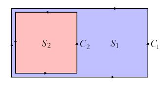
(a)

(b)

Figure 1: (a) a “coplanar” double-winding Wilson loop, (b) a “shifted” double-winding Wilson loop.

The area dependence of the expectation value $\langle W(C_{1}\cup C_{2})\rangle$ has been first investigated in [1] to show that the coplanar double-winding Wilson loop average obeys the “difference-of-areas law” in the lattice $SU(2)$ Yang-Mills model by using the strong coupling expansion and the numerical simulations:

$${\langle W(C_{1}\cup C_{2})\rangle}_{R=0}\simeq\exp[-\sigma||S_{1}|-|S_{2}||]\ ,$$ (2)

where $S_{1}$ and $S_{2}$ are respectively the minimal areas bounded by loops $C_{1}$ and $C_{2}$.

In the continuum $SU(N)$ Yang-Mills model, general multiple-winding Wilson loops have been investigated in [2] to show that there is a novel “max-of-areas law” which is neither difference-of-areas law nor sum-of-areas law for multiple-winding Wilson loop average, provided that the string tension obeys the Casimir scaling for quarks in the higher representations.

In the lattice $SU(N)$ Yang-Mills model, it has been shown in [3] that the coplanar double-winding Wilson loop average has the $N$-dependent area law falloff in the strong coupling region: “difference-of-areas law” for $N=2$, “max-of-areas law” for $N=3$ and “sum-of-areas law” for $N\geqslant 4$:

$${\langle W(C_{1}\cup C_{2})\rangle}_{R=0}\simeq\begin{cases}\exp[-\sigma||S_{1}|-|S_{2}||]&(N=2)\\ \exp[-\sigma\max(|S_{1}|,|S_{2}|)]&(N=3)\\ \exp[-\sigma(|S_{1}|+|S_{2}|)]&(N\geqslant 4)\end{cases}\ .$$ (3)

Moreover, a shifted double-winding Wilson loop average as a function of the distance $R$ in a transverse direction has the long distance behavior which does not depend on $N$, while the short distance behavior depends on $N$.

In our investigation in [4], we examine the center group dominance for a double winding Wilson loop average. It has been shown in [5] that the ordinary single-winding Wilson loop average in the non-Abelian lattice gauge theory with the gauge group $G$ is bounded from above by the same Wilson loop average in the Abelian lattice gauge theory with the center gauge group $Z(G)$:

$$|\langle W_{R(G)}(C)\rangle_{G}(\beta)|\leq 2{\rm tr}({\bf 1})\langle W_{R(Z(G))}(C)\rangle_{Z(G)}(2{\rm dim}(G)\beta)\ .$$ (4)

We have extended the above statement to the double winding Wilson loop average, beyond the case of the ordinary single-winding Wilson loop average:

$$|\langle W_{R(G)}(C_{1}\cup C_{2})\rangle_{G}(\beta)|\leq 2{\rm tr}({\bf 1})\langle W_{R(Z(G))}(C_{1}\cup C_{2})\rangle_{Z(G)}(2{\rm dim}(G)\beta)\ .$$ (5)

From this point of view, we introduce the character expansion to the weight ${e}^{S_{G}[U]}$ coming from the action and perform the group integration, in order to estimate the expectation value in the $Z_{N}$ lattice gauge model. We evaluate the double-winding Wilson loop average up to the leading contribution to show that the $N$-dependent area law falloff in the $SU(N)$ lattice gauge model can be reproduced by using the (Abelian) $Z_{N}$ lattice gauge model. By taking the limit $N\to\infty$, we show the center group dominance for a double-winding Wilson loop average in the $U(N)$ lattice gauge model through the $U(1)$ lattice gauge model.

Finally, we extend the above arguments for the lattice gauge-scalar model on the “analytic region”. For this purpose, we estimate the area law falloff, the string tension, and the mass gap by using the cluster expansion.

2 Lattice $Z_{N}$ gauge model

First, we consider the lattice $Z_{N}$ gauge model with the coupling constant defined by $\beta:=1/g^{2}$ on a $D$-dimensional lattice $\Lambda$ with unit lattice spacing, which is specified by the action

$$S_{G}[U]=\beta\sum_{p\in\Lambda}\mathrm{Re}\ U_{p}\ ,\quad U_{p}:=\prod_{\ell\in\partial p}{U}_{\ell}\ ,$$ (6)

where $\ell$ labels a link, $p$ labels an elementary plaquette. To examine this $Z_{N}$ gauge model analytically, we introduce the character expansion to the weight ${e}^{S_{G}[U]}$ to obtain the expanded form of the expectation value of an operator $\mathscr{F}$:

$${\langle\mathscr{F}\rangle}_{\Lambda} :={Z}_{\Lambda}^{-1}\int\prod_{\ell\in\Lambda}d{U}_{\ell}\ {e}^{S_{G}[U]}\mathscr{F}={Z}_{\Lambda}^{-1}\int\prod_{\ell\in\Lambda}d{U}_{\ell}\ \prod_{p\in\Lambda}\sum_{n=0}^{N-1}b_{n}(\beta)U_{p}^{n}\mathscr{F}\ ,$$ (7)

$${Z}_{\Lambda} :=\int\prod_{\ell\in\Lambda}d{U}_{\ell}\ {e}^{S_{G}[U]}\ ,$$ (8)

where the coefficients $b_{n}(\beta)$ is defined by

$$b_{n}(\beta):=\frac{1}{N}\sum_{\zeta\in Z_{N}}{\zeta}^{-n}{e}^{\beta\mathrm{Re}\ \zeta}\ .$$ (9)

We define $c_{n}(\beta):=b_{n}(\beta)/b_{0}(\beta)$. For $N=2,3,4$ and $\infty$, $c_{1}(\beta)$ and $c_{2}(\beta)$ are written in the form

$$c_{1}(\beta) =\frac{{e}^{\beta}-{e}^{-\beta}}{{e}^{\beta}+{e}^{-\beta}}\quad(N=2)\ ,\qquad c_{1}(\beta)=\frac{{e}^{\beta}-{e}^{-\beta/2}}{{e}^{\beta}+2{e}^{-\beta/2}}=c_{2}(\beta)\quad(N=3)\ ,$$

$$c_{1}(\beta) =\frac{{e}^{\beta}-{e}^{-\beta}}{{e}^{\beta}+2+{e}^{-\beta}},\quad c_{2}(\beta)=\frac{{e}^{\beta}-2+{e}^{-\beta}}{{e}^{\beta}+2+{e}^{-\beta}}\quad(N=4)\ ,$$

$$c_{1}(\beta) =\frac{I_{1}(\beta)}{I_{0}(\beta)},\quad c_{2}(\beta)=\frac{I_{2}(\beta)}{I_{0}(\beta)}\quad(N=\infty)\ .$$ (10)

Note that ${b}_{N-n}(\beta)=b_{n}(\beta)$ and $0\leqslant c_{n}(\beta)<1$ for $0\leqslant\beta<\infty$. For $N=2,3,4$ and $\infty$ , the behavior of $c_{1}(\beta)$ and $c_{2}(\beta)$ as functions of $\beta$ are indicated in Fig.2. We find that $c_{1}(\beta)\sim\mathcal{O}(\beta)\ (N\geqslant 2)$ and $c_{2}(\beta)\sim\mathcal{O}({\beta}^{2})\ (N\geqslant 4)$ for $\beta\ll 1$.

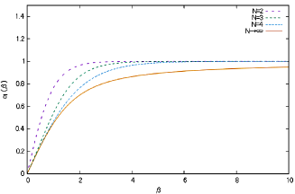
(a) $c_{1}(\beta)\ (N=2,3,4,\infty)$

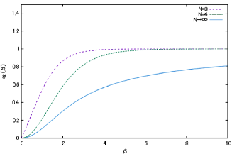
(b) $c_{2}(\beta)\ (N=3,4,\infty)$

Figure 2: The character expansion coefficient as a function of $\beta$, (a) $c_{1}(\beta)$,  (b) $c_{2}(\beta)$

Next, we evaluate the expectation value of a coplanar double-winding Wilson loop in the lattice $Z_{N}$ pure gauge model. The leading contribution to a coplanar double-winding Wilson loop average is given by the tiling of a planar set of plaquettes, as shown in the Fig.3. (These result are exact for all $\beta$ when $D=2$, while valid for $\beta\ll 1$ when $D>2$.)

(a) $N=2$

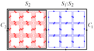
(b) $N\geqslant 3$

Figure 3: A coplanar double-winding Wilson loop, (a) $N=2$ ,  (b) $N\geqslant 3$

The result of the coplanar double-winding Wilson loop average up to the leading contribution is given by

$${\langle W(C_{1}\cup C_{2})\rangle}_{R=0}\simeq\begin{cases}{c_{1}(\beta)}^{|S_{1}|-|S_{2}|}&(N=2)\\ {c_{1}(\beta)}^{|S_{1}|}&(N=3)\\ {c_{2}(\beta)}^{|S_{2}|}{c_{1}(\beta)}^{|S_{1}|-|S_{2}|}&(N\geqslant 4)\end{cases}\ .$$ (11)

Then we obtain the (non-zero) string tension from this result:

$$\sigma(\beta)\simeq\ln\frac{1}{c_{1}(\beta)}>0\ .$$ (12)

In the strong coupling region, this result reproduces the area law falloff in the $SU(N)$ lattice gauge model obtained in [3]. Moreover, by taking the continuous group limit $N\to\infty$ ,we find that the area law for $N\geqslant 4$ persists in the $U(1)$ lattice gauge model.

Furthermore, we also evaluate the expectation value of a shifted double-winding Wilson loop in the lattice $Z_{N}$ pure gauge model. The leading contribution to a shifted double-winding Wilson loop average can be given by the 2 types of tiling by a set of plaquettes, as shown in the Fig.4.

(a) $R$-independent contribution

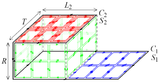
(b) $R$-dependent contribution

Figure 4: A shifted double-winding Wilson loop, (a) $R$-independent contribution, (b) $R$-dependent contribution

The result of the shifted double-winding Wilson loop average up to the leading contribution is given by

$${\langle W(C_{1}\cup C_{2})\rangle}_{R\neq 0}\simeq\begin{cases}{c_{1}(\beta)}^{|S_{1}|+|S_{2}|}+{c_{1}(\beta)}^{2R(L_{2}+T)}\cdot{c_{1}(\beta)}^{|S_{1}|-|S_{2}|}&(N=2)\\ {c_{1}(\beta)}^{|S_{1}|+|S_{2}|}+{c_{1}(\beta)}^{2R(L_{2}+T)}\cdot{c_{1}(\beta)}^{|S_{1}|}&(N=3)\\ {c_{1}(\beta)}^{|S_{1}|+|S_{2}|}+{c_{1}(\beta)}^{2R(L_{2}+T)}\cdot{c_{2}(\beta)}^{|S_{2}|}{c_{1}(\beta)}^{|S_{1}|-|S_{2}|}&(N\geqslant 4)\end{cases}\ .$$ (13)

This result reproduces the $R$-dependent behavior of the shifted double-winding Wilson loop average in [3]. In particular, we obtain the (non-zero) mass gap from the case of $S_{1}=S_{2}=1$ and $R\gg 1$ in the above result:

$$\Delta(\beta)=4\ln\frac{1}{c_{1}(\beta)}>0\ .$$ (14)

3 Lattice $Z_{N}$ gauge-scalar theory

Next, we consider the lattice $Z_{N}$ gauge-scalar model with the frozen scalar field norm $R$ for simplicity. The action of this model with the coupling constants defined by $\beta:=1/g^{2}$ and $K:=R^{2}$ on a $D$-dimensional lattice $\Lambda$ with unit lattice spacing is given by

$$S[U,\varphi]=\beta\sum_{p\in\Lambda}\mathrm{Re}\ U_{p}+K\sum_{\ell\in\Lambda}\mathrm{Re}\left({\varphi}_{x}{U}_{\ell}{\varphi}_{x+\ell}^{*}\right)\ ,$$ (15)

where $\ell$ labels a link, and $p$ labels an elementary plaquette. ${U}_{\ell}$ is a $Z_{N}$ link variable on link $\ell$ and ${\varphi}_{x}$ is a $Z_{N}$ scalar field at site $x$ which transforms according to the fundamental representation of the gauge group $Z_{N}$.

In this model, the expectation value of an operator $\mathscr{F}$ has the form

$${\langle\mathscr{F}\rangle}_{\Lambda} :={Z}_{\Lambda}^{-1}\int\prod_{\ell\in\Lambda}d{U}_{\ell}\prod_{x\in\Lambda}d{\varphi}_{x}\ {e}^{S[U,\varphi]}\mathscr{F}={Z}_{\Lambda}^{-1}\int\prod_{\ell\in\Lambda}d{U}_{\ell}\ h[U]\ {e}^{\beta\sum_{p\in\Lambda}\mathrm{Re}\ U_{p}}\mathscr{F}\ ,$$

$${Z}_{\Lambda} :=\int\prod_{\ell\in\Lambda}d{U}_{\ell}\prod_{x\in\Lambda}d{\varphi}_{x}\ {e}^{S[U,\varphi]}\ ,\quad h[U]:=\int\prod_{x\in\Lambda}d{\varphi}_{x}\ {e}^{K\sum_{\ell\in\Lambda}\mathrm{Re}({\varphi}_{x}{U}_{\ell}{\varphi}_{x+\ell}^{*})}\ .$$ (16)

According to [6], we can perform the cluster expansion by introducing the new variable ${\rho}_{p}$ and the new measure $d{\mu}_{\Lambda}$ which absorbs the scalar part $h[U]$:

$${\langle\mathscr{F}\rangle}_{\Lambda} =\frac{\int d{\mu}_{\Lambda}\prod_{p\in\Lambda}\left(1+{\rho}_{p}\right)\mathscr{F}}{\int d{\mu}_{\Lambda}\prod_{p\in\Lambda}\left(1+{\rho}_{p}\right)}=\sum_{Q(Q_{0})\subset\Lambda}\int d{\mu}_{\Lambda}\ \mathscr{F}\prod_{p\in Q(Q_{0})}{\rho}_{p}\cdot\frac{{Z}_{{[Q(Q_{0})\cup Q_{0}]}^{c}}}{{Z}_{\Lambda}}\ ,$$ (17)

$$d{\mu}_{\Lambda} :=\frac{\prod_{\ell\in\Lambda}d{U}_{\ell}\ h[U]}{\int\prod_{\ell\in\Lambda}d{U}_{\ell}\ h[U]}\ ,\quad{\rho}_{p}:={e}^{\beta\mathrm{Re}\ U_{p}}-1\ ,$$ (18)

where $Q_{0}$ is the set of plaquettes which is the support of $\mathscr{F}$ and $Q(Q_{0})$ is the set of plaquettes which is connected to $Q_{0}$. For the general set of plaquettes $Q$, $Q^{c}$ represents the complement of $Q$. Here, $Z_{Q}$ is defined by

$${Z}_{Q}:=\sum_{Q^{\prime}\subset Q}\int d{\mu}_{\Lambda}\prod_{p\in Q^{\prime}}{\rho}_{p}\ .$$ (19)

Note that ${\rho}_{p}\sim\mathcal{O}(\beta)$ for $\beta\ll 1$. It has been showed in [7] that the confinement region ($0\leqslant\beta\ll 1,K\ll 1$) and the Higgs region ($\beta\gg 1,K_{c}\leqslant K<\infty$) are analytically continued in a single “analytic region”, where the cluster expansion converges uniformly. See Fig.5.

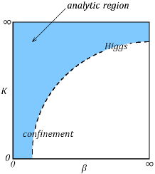
Figure 5: The analytic region on the $\beta$-$K$ plane

To evaluate $h[U]$, we apply the character expansion and perform the group integration. Ignoring the contributions from multiple plaquettes, then we obtain the expression which is valid up to the lowest plaquettes order:

$$h[U] =\int\prod_{x\in\Lambda}d{\varphi}_{x}\prod_{\ell\in\Lambda}\left[b_{0}(K)+b_{1}(K){\varphi}_{x}{U}_{\ell}{\varphi}_{x+\ell}^{*}+\cdots+{b}_{N-1}(K){\left({\varphi}_{x}{U}_{\ell}{\varphi}_{x+\ell}^{*}\right)}^{N-1}\right]$$

$$={N}^{|\Lambda|}{b_{0}(K)}^{D|\Lambda|}\prod_{p\in\Lambda}\sum_{n=0}^{N-1}{c_{n}(K)}^{4}U_{p}^{n}+\cdots\ .$$ (20)

We estimate the leading contribution to the double-winding Wilson loop average with the above $h[U]$, we also apply the character expansion for ${\rho}_{p}$ and evaluate the upper bound of the cluster expansion by using the binominal expansion. We find that there is an correspondence between the evaluation for the $Z_{N}$ lattice gauge model and for the estimated upper bound for the $Z_{N}$ lattice gauge-scalar model:

$$c_{n}(\beta)\mapsto a_{n}(\beta,K):= \frac{\left[b_{0}(\beta)-{e}^{\beta}\right]{c_{n}(K)}^{4}+b_{1}(\beta){{c}_{n+1}(K)}^{4}+\cdots+{b}_{N-1}(\beta){{c}_{N+n-1}(K)}^{4}}{b_{0}(\beta)+b_{1}(\beta){c_{1}(K)}^{4}+\cdots+{b}_{N-1}(\beta){{c}_{N-1}(K)}^{4}}+{c_{n}(K)}^{4}\ .$$

$$(\mod N\ ,\ n=1,\cdots,N-1)$$ (21)

Note that $a_{n}(\beta,0)=c_{n}(\beta)$ and $a_{n}(\beta,\infty)=1$. The above estimation is valid only for the values of parameter $\beta$ and $K$ on the analytic region in the range where the string breaking does not occur.

By applying the same method as the above, we obtain the estimation for the coplanar double-winding Wilson loop average:

$${\langle W(C_{1}\cup C_{2})\rangle}_{R=0}\lesssim\begin{cases}{a_{1}(\beta,K)}^{|S_{1}|-|S_{2}|}&(N=2)\\ {a_{1}(\beta,K)}^{|S_{1}|}&(N=3)\\ {a_{2}(\beta,K)}^{|S_{2}|}{a_{1}(\beta,K)}^{|S_{1}|-|S_{2}|}&(N\geqslant 4)\end{cases}$$ (22)

and we obtain the (non-zero) string tension from the above result:

$$\sigma(\beta,K)\gtrsim\ln\frac{1}{a_{1}(\beta,K)}>0\ .$$ (23)

This estimation suggests that the area law falloff in the $Z_{N}$ lattice gauge model persists in the $Z_{N}$ lattice gauge-scalar model and the $K\to 0$ limit agrees with the pure gauge case. Moreover, for $\sigma(\beta,K)$, the $K\to 0$ limit agrees with $\sigma(\beta)$ in the $Z_{N}$ lattice gauge model, and $K\to\infty$ limit converges to 0 uniformly in $\beta$. In other words, the string tension is non-zero on the analytic region.

Additionally, we also estimate the shifted double-winding Wilson loop average:

$${\langle W(C_{1}\cup C_{2})\rangle}_{R\neq 0}$$

$$\quad\lesssim\begin{cases}{a_{1}(\beta,K)}^{|S_{1}|+|S_{2}|}+{a_{1}(\beta,K)}^{2R(L_{2}+T)}\cdot{a_{1}(\beta,K)}^{|S_{1}|-|S_{2}|}&(N=2)\\ {a_{1}(\beta,K)}^{|S_{1}|+|S_{2}|}+{a_{1}(\beta,K)}^{2R(L_{2}+T)}\cdot{a_{1}(\beta,K)}^{|S_{1}|}&(N=3)\\ {a_{1}(\beta,K)}^{|S_{1}|+|S_{2}|}+{a_{1}(\beta,K)}^{2R(L_{2}+T)}\cdot{a_{2}(\beta,K)}^{|S_{2}|}{a_{1}(\beta,K)}^{|S_{1}|-|S_{2}|}&(N\geqslant 4)\end{cases}$$ (24)

and we obtain the (non-zero) mass gap from the case of $S_{1}=S_{2}=1$ and $R\gg 1$ in the above result:

$$\Delta(\beta,K)\gtrsim 4\ln\frac{1}{a_{1}(\beta,K)}>0\ .$$ (25)

For $\Delta(\beta,K)$, the $K\to 0$ limit agrees with $\Delta(\beta)$ in the $Z_{N}$ lattice gauge model, and $K\to\infty$ limit converges to 0 uniformly in $\beta$. In other words, the mass gap is non-zero on the analytic region.

4 Conclusion

We investigated the area law falloff of the double-winding Wilson loops in the $Z_{N}$ lattice gauge model and $Z_{N}$ lattice gauge-scalar model, where the gauge group is the center group of the original $SU(N)$. First, we evaluated the $N$-dependent area law falloff for the coplanar double-winding Wilson loop average up to the leading contribution. We found the $N$-dependence of the area law falloff in the $Z_{N}$ lattice gauge model, which reproduces the area law falloff in the $SU(N)$ lattice gauge model obtained in [3]. Secondly, we also checked the limit $N\to\infty$, the area law falloff for $N\geqslant 4$ persists in the $U(1)$ lattice gauge model. This result implies that the coplanar double-winding Wilson loop average in the $U(N)$ lattice gauge model and the $SU(N)(N\geqslant 4)$ lattice gauge model obeys the same area law up to the leading contribution. Furthermore, we also considered the shifted double-winding Wilson loop average up to the leading contributions. This result reproduces the $R$-dependent behavior in the $SU(N)$ lattice gauge model obtained in [3]. We obtained the (non-zero) mass gap $\Delta(\beta)$ from this result. Finally, we extended the above study for the $Z_{N}$ lattice gauge-scalar model on the analytic region. We found that the area law falloff in the $Z_{N}$ lattice gauge model persists in the $Z_{N}$ lattice gauge-scalar model. We discovered that the string tension and the mass gap are non-zero on the analytic region from this estimation.

References

[1]
J. Greensite and R. Höllwieser,
Phys. Rev. D91, 054509 (2015)
[arXiv:1411.5091 [hep-lat]]
[2]
R. Matsudo and K.-I. Kondo,
Phys. Rev. D96, 105011 (2017)
[arXiv:1706.05665 [hep-th]]
[3]
S. Kato, A. Shibata and K.-I. Kondo,
Phys.Rev. D102, 094521 (2020) [arXiv:2008.03684 [hep-lat]]
[4]
R. Ikeda and K.-I. Kondo,
Prog. Theor. Exp. Phys. 2021, ptab114 (2021)
[arXiv:2106.14416 [hep-lat]]
[5]
J. Fröhlich,
Phys. Lett. 83B, 195 (1979).
[6]
K. Osterwalder and E. Seiler,
Annals Phys. 110, 440 (1978).
[7]
E.H. Fradkin and S.H. Shenker,
Phys.Rev. D19, 3682–3697 (1979).