Tensor Deblurring and Denoising Using Total Variation

Abstract

We consider denoising and deblurring problems for tensors. While images can be discretized as matrices, the analogous procedure for color images or videos leads to a tensor formulation. We extend the classical ROF functional for variational denoising and deblurring to the tensor case by employing multi-dimensional total variation regularization. Furthermore, the resulting minimization problem is calculated by the FISTA method generalized to the tensor case. We provide some numerical experiments by applying the scheme to the denoising, the deblurring, and the recoloring of color images as well as to the deblurring of videos.

1 Introduction

Digital image restoration is an important task in image processing since it can be applied to various areas of applied sciences such as medical and astronomical imaging, film restoration, and image and video coding. There are already various methods (most of them not tensor-based) to recover signal/images from noise and blurry observations, for instance, statistical-based approaches [5, 6], methods employing Fourier and/or wavelet transforms [8, 7], or variational methods [10, 9]. Among the variational methods, total variation (TV) regularization is one of the most prominent examples. TV regularization, first introduced by Rudin, Osher, and Fatemi (ROF) in 1992 [4], has become one of the most used techniques in image processing and computer vision because it is known to remove noises while preserving sharp edges and boundaries. It has since evolved from an image denoising method into a more general technique applied to various inverse problems such as deblurring, blind deconvolution, and inpainting. The results in this article are an extension to tensors of the ROF methodology and the techniques describe by Teboulle and Beck in [3]. Teboulle and Beck’s approach was to minimize the TV-functional using gradient projection, proximal mappings and Nestorov acceleration, applied to the dual functional of ROF that was proposed by Chambolle in [11, 12]. Here we extend these algorithms to multi-channel images and videos. After discretization, these objects can be represented as tensors. For simplicity, most formulas that we present are for third-order tensors. However, keep in mind that this work can be extended to any n-th order tensor with little effort.

We provide some details for the total variation functional in Section 2, describe the minimization algorithms that we use in Section 3, and then present our numerical approach for the denoising and deblurring for tensors using total variation in the subsequent sections. We will provide some numerical results to prove the effectiveness of our approach using colored images and videos.

2 Definition and Preliminaries

Recall that in image denoising, the preservation of certain visible structure such as edges is essential. To achieve that goal, various methods were proposed like wavelet-based methods, stochastic methods, and variational methods, in particular, total variation regularization.

The Rudin-Osher-Fatemi (ROF) model for denoising to obtain a clean image $u$ from a noisy one $f$ proposes to solve the following optimization problem:

(1) $$\min_{u\in BV(\Omega)}\|u\|_{TV(\Omega)}+\frac{\lambda}{2}\|f-u\|^{2}_{L^{2}}\,dx,$$

where $BV(\Omega)$ is the set of functions with bounded variation over the domain $\Omega$, $TV(\Omega)$ is the total variation over the domain, and $\lambda$ is a penalty parameter. The functional in Eq. 1 is defined in the space of functions of bounded variation, so it does not necessarily require image functions to be continuous and smooth. That is why the denoised image allows for jumps or discontinuities, i.e., edges, and the visual quality of the result is superior to linear filter methods.

The ROF formulation do have some weaknesses like that it is not strictly convex, it is susceptible to backward diffusion, and it favors piecewise constant solutions, which may cause false edges (staircases) in the output image; see [23]. Also, in a naive numerical approach to minimize (1), one has to add some small regularization parameter to calculate the derivative of $\|u\|_{TV(\Omega)}$ [18, 19, 20], which can result in some loss in accuracy.

Furthermore, although the ROF formulation is efficient in preserving edges of uniform and small curvature, it may result in excessively smoothening of small scale features having more pronounced curvature edges as shown in [21]. As Chan et al. explained in [22, 23, 24], the TV approach may sometimes result in loss of contrast and geometry in the output images, even when the observed image is noise-free.

However, given the strength of TV-based techniques, especially in edge preservation, various approach have been proposed to solve the above mentioned issues, for instance, the total variation penalty method by Vogel in [19, 25] or the adaptive total variation based regularization model by Strong and Chan [26]. Recently, many researchers have employed algorithms that use the dual formulation of the ROF model; see [28, 27, 11].

In the original formulation, the isotropic TV seminorm $\|u\|_{TV(\Omega)}$ is used, which essentially is the $L^{1}(\Omega)$-norm of the Euclidean norm of the gradient of a function (extended to nondifferentiable functions by a weak formulation).

However, the isotropic TV can sometimes round the sharp edges of an image such as at corners points. To overcome this, a modification of the ROF model Eq. 1, the anisotropic TV, was pointed out by Esedoglu and Osher [13]. Anisotropic TV helps avoid blur at the corners, and the difference to the isotropic case is the use of the $\ell^{1}$-norm of the gradient in place of the Euclidean norm.

For numerical computations, only discretized versions of the ROF-functionals are needed. More precisely, after discretization, the image $f$ and the denoised image $u$ in (1) can be regarded as matrices in $\mathbb{R}^{m\times n}$. Let us denote the isotropic TV by $TV_{I}$ and the anisotropic TV by $TV_{L_{1}}$. The discrete version of the TV-seminorms read as follows:

(2) $$\begin{split}&TV_{I}=\sum_{i=1}^{m-1}\sum_{j=1}^{n-1}\sqrt{(x_{i,j}-x_{i+1,j})^{2}+(x_{i,j}-x_{i,j+1})^{2}}\\ \end{split}$$

The anisotropic Total Variation seminorm on the other hand is defined as

(3) $$\begin{split}TV_{L_{1}}(x)=&\sum_{i=1}^{m-1}\sum_{j=1}^{n}\mid x_{i+1,j}-x_{i,j}\mid+\sum_{i=1}^{m}\sum_{j=1}^{n-1}\mid x_{i,j+1}-x_{i,j}\mid\,.\end{split}$$

Our approach works for either isotropic or anisotropic TV.

One of the objectives of the current article is to extend the ROF-formulation from the image case to the tensor case. That is, we consider inputs $f$ and denoised elements $u$ as being 3rd-order tensor, i.e., elements in $\mathbb{R}^{m\times n\times o}$ (or more general, $n$-th order tensors). These can be seen as discretizations of 3-variate functions (e.g., gray-scale images depending on time or color images).

Let us briefly sketch our tensor notation. We denote a vector by a bold lower-case letter $\mathbf{a}$. The bold upper-case letter ${A}$ represents a matrix, and the symbol of a tensor is a calligraphic letter $\mathcal{A}$. Throughout this paper, we focus primarily on third-order and fourth-order tensors, $\mathcal{A}=(a_{ijk})\in\mathbb{R}^{I\times J\times K}$ and $\mathcal{A}=(a_{ijkl})\in\mathbb{R}^{I\times J\times K\times L}$, respectively, of indices $1\leq i\leq I,1\leq j\leq J$ and $1\leq l\leq K$, but all definitions and calculations are applicable to tensors of any order $n>2$. In some calculations, tensor unfolding (a.k.a matricization) is required.

A third-order tensor $\mathcal{A}$ has column, row and tube fibers, which are defined by fixing every index but one and denoted by ${a}_{:jk}$, ${a}_{i:k}$ and ${a}_{ij:}$ respectively. Correspondingly, we can obtain three kinds of matricizations ${A}_{(1)}\in\mathbb{R}^{I\times J\cdot K},{A}_{(2)}\in\mathbb{R}^{J\times I\cdot K}$, and ${A}_{(3)}\in\mathbb{R}^{K\times I\cdot J}$ of $\mathcal{A}$ according to respectively arranging the column, row, and tube fibers to be columns of matrices.

The inner product of $\mathcal{S}\in\mathbb{R}^{I\times J\times K}$ and $\mathcal{T}\in\mathbb{R}^{I\times J\times K}$ is given by

$$\langle\mathcal{S},\mathcal{T}\rangle=\sum_{ijk}s_{ijk}t_{ijk}.$$

The inner product for third-order tensors is easily generalized to $n$th-order tensors; i.e., $\langle\mathcal{S},\mathcal{T}\rangle=\sum_{i_{1}i_{2}\cdots i_{n}}s_{i_{1}i_{2}\cdots i_{n}}t_{i_{1}i_{2}\cdots i_{n}}$.

The contracted product can be viewed as a partial inner product in multiple indices. For example, given a third-order tensor $\mathcal{S}\in\mathbb{R}^{I\times J\times K}$ and a second-order tensor $A\in\mathbb{R}^{J\times K}$, we define the contracted product as

$$\langle\mathcal{S},{A}\rangle_{2,3;1,2}=\sum_{jk}s_{ijk}a_{jk},$$

where the modes 2, 3 and 1, 2 indicate the indices that are being contracted. In general, given any two tensors, $\mathcal{S}\in\mathbb{R}^{I_{1}\times I_{2}\cdots\times I_{M}}$ and $\mathcal{A}\in\mathbb{R}^{J_{1}\times J_{2}\cdots\times J_{N}}$, then the contracted product in the modes, $\bar{i}_{1},\bar{i}_{2},\cdots\bar{i}_{l}$, where $\bar{i}_{l}\in[1,\cdots,M]$ and $\bar{j}_{1},\bar{j}_{2},\cdots\bar{j}_{l}$, where $\bar{j}_{l}\in[1,\cdots,N]$ is defined as

$$\langle\mathcal{S},\mathcal{A}\rangle_{\bar{i}_{1},\bar{i}_{2}\cdots\bar{i}_{l};\bar{j}_{1},\bar{j}_{2}\cdots\bar{j}_{l}}=\sum_{k_{1},\cdots,k_{l}}s_{i_{1}i_{2}k_{1}i_{3}k_{2}\cdots i_{M-2}k_{l-1}k_{l}i_{M}}a_{k_{1}j_{2}k_{2}\cdots j_{M-2}k_{l-1}k_{l}},$$

where $k_{m}$ represents the index corresponding to the contracting mode pair $(\bar{i}_{m},\bar{j}_{m})$ given that the $i_{m}$ and $j_{m}$ indices are not contracting modes.

The Frobenius norm of a tensor is given by

$$\|\mathcal{S}\|_{F}=\langle\mathcal{S},\mathcal{S}\rangle^{1/2},$$

where $\mathcal{S}\in\mathbb{R}^{I\times J\times K}$.

The element-wise multiplication and division of two tensors $\mathcal{X}\in\mathbb{R}^{I\times J\times K}$ and $\mathcal{Y}\in\mathbb{R}^{I\times J\times K}$ are defined as

$$\mathcal{X}\cdot*\mathcal{Y}=x_{ijk}y_{ijk}$$

and

$$\mathcal{X}\cdot/\mathcal{Y}=\frac{x_{ijk}}{y_{ijk}},$$

respectively.

3 Minimization algorithms: ISTA, FISTA, and MFISTA

In this section, we describe the algorithms that are used to minimize the TV-regularization functional.

Consider the following optimization problem:

(4) $$\min\{G(x)\equiv f(x)+g(x)\},$$

where $f$ and $g$ are functionals with certain properties that are specified below.

3.1 Iterative Shrinkage/Thresholding Algorithm (ISTA)

ISTA (Iterative Shrinkage/Thresholding algorithm) is an iterative method for minimizing problems of the form (4) in the case when $g$ is convex but not necessarily differentiable and $f$ is differentiable with Lipschitz continuous gradient. It involves a combination of a usual gradient step for $f$ and a proximal operator with respect to $g$.

This algorithm can be traced back to the proximal forward-backward iterative scheme introduced by Bruck in 1975 [37] and Passty in 1979 [38] within the general framework of splitting methods. Since the optimization problem Eq. 4 involves a minimization of a sum of a smooth term and a nonsmooth term, the ISTA model splits the minimization of $f$ and $g$, and it iteratively calculates a minimizing sequence by

(5) $${x}_{n+1}=\arg\min\limits_{{x}}\left\{f({x}_{n})+\langle{x}-{x}_{n},\nabla f({x}_{n})\rangle+\frac{L}{2}\|{x}-{x}_{n}\|^{2}+g({x})\right\},$$

where $f$ and $g$ are the smooth and nonsmooth functions, respectively.

The iteration can be written as

$${x}_{n+1}=p_{L}({x}_{n}),\qquad p_{L}({x}_{n})=(I+\tfrac{1}{L}\partial g)^{-1}\left({x}_{n}-\tfrac{1}{L}\nabla f(\mathbf{x}_{n}\right).$$

Here, $\partial g$ is the subgradient of $g$. In Eq. 4 if $g(x)\equiv 0$, then ISTA is reduced to a smooth gradient method. ISTA has a worst-case convergence rate of $O(1/k)$ [1]. The algorithms is summarized in Algorithm 1.

Algorithm 1 ISTA

0:  $L\coloneqq L(f)$, where L is a Lipschitz constant of $\nabla(f)$.Step 0. Take $x_{0}\in\mathbb{R}^{n}$Step n. ($n\geq 1$) Compute

$$x_{n}=p_{L}\left(x_{n-1}\right)$$

3.2 Fast Iterative Shrinkage/Thresholding Algorithm (FISTA)

Nesterov in [15] showed that for smooth optimzation problems, there exists a gradient method with an $O(1/k^{2})$ convergence rate, which is a substantial improvement compared to the rate for, e.g., ISTA. The method of Nesterov (Nesterov’s acceleration) only requires one gradient evaluation at each iteration and involves an additional recombination step with the previous iterate, which is easy to compute. FISTA is an extention of Nesterov’s acceleration [15] to the problem in Eq. 4; the method is described in Algorithm 2.

Algorithm 2 FISTA

0:  An upper bound $L\geq L(f)$ on the Lipschitz constant L(f) of $\nabla(f)$.Step 0. Take $y_{1}=x_{0}\in\mathbb{R}^{n}$, $t_{1}=1$Step n. ($n\geq 1$) Compute

(6) $$x_{n}=p_{L}\left(y_{n}\right)$$

(7) $$t_{n+1}=\frac{1+\sqrt{1+4t_{n}^{2}}}{2}$$

(8) $$y_{n+1}=x_{n}+\left(\frac{t_{n}-1}{t_{n+1}}\right)\left(x_{n}-x_{n-1}\right)$$

The main difference between the FISTA and ISTA is that the operator $p_{L}(\cdot)$ is not employed at the previous point $x_{k-1}$ but rather at the point $y_{k}$ that is a linear combination of the previous two iterates {$x_{k-1},x_{k-2}$}. Each iterate of FISTA depends on the previous two iterates and not only on the last iterate as in ISTA. Note that FISTA is as simple as ISTA. They both share the same computational demand; the computation of the remaining additional steps is computationally negligible. Convergence of the FISTA algorithm was shown in [1]; we state the main convergence result for FISTA in 1.

Theorem 1 ([1], Theorem 4.1).

Let $\{x_{k}\}$ be generated by FISTA. Then for any $k\geq 1$

$$F(x_{k})-F(x^{*})\leq\frac{2L\|x_{0}-x^{*}\|^{2}}{(k+1)^{2}},\qquad\forall x^{*}\in X^{*}.$$

Contrary to ISTA, FISTA is not a monotone algorithm, i.e., the functional values are not necessarily monotonically decreasing. Although it is not required for convergence, monotonicity is a desirable property. Especially when an inexact version of FISTA is used, e.g., when the proximal mapping is only available approximately, monotonicity makes the alogorithms become more robust. This issue brought the monotone version of FISTA, called MFISTA, which is described in Algorithm 3. The convergence result for MFISTA remain the same as for FISTA:

Theorem 2 ([3], Theorem 5.1).

Let $\{x_{k}\}$ be generated by FISTA. Then for any $k\geq 1$

$$F(x_{k})-F(x^{*})\leq\frac{2L\|x_{0}-x^{*}\|^{2}}{(k+1)^{2}},\qquad\forall x^{*}\in X^{*}.$$

Algorithm 3 MFISTA [3]

0:  $L\geq L(f)$, where L is an upper bound on the Lipschitz constant of $\nabla(f)$.Step 0. Take $y_{1}=x_{0}\in\mathbb{R}^{n}$, $t_{1}=1$Step n. ($n\geq 1$) Compute

$$x_{n}=p_{L}\left(y_{n}\right)$$

$$t_{n+1}=\frac{1+\sqrt{1+4t_{n}^{2}}}{2}$$

$$x_{n}=\operatorname*{argmin}\{F(x):x=z_{n},x_{n-1}\}$$

$$y_{n+1}=x_{n}+\left(\frac{t_{n}}{t_{n+1}}\right)(z_{n}-x_{n})+\left(\frac{t_{n}-1}{t_{n+1}}\right)\left(x_{n}-x_{n-1}\right)$$

Employing FISTA for the ROF problem is at first sight an obvious task by setting $g(x)=TV(x)$ and $f(x)=\frac{\lambda}{2}\|x-f\|^{2}$. However, this leads to the difficulty of calculating the proximal mapping $(I+\partial g)^{-1}$ for $g$, which is not at all easy to do. Instead, it was proposed in [3] to apply FISTA to the dual ROF problem. The dual problem has been identified and proposed by Chambolle [11, 12] and essentially reads as

$$\min_{p}\|f-\mbox{div}\,p\|^{2}:\quad\text{s.t.}\ \|p\|_{L^{\infty}}\leq 1.$$

Thus, we may use for $g(x)$ in the FISTA scheme, the indicator function of $\|p\|_{L^{\infty}}\leq 1$. The corresponding proximal mapping can be calculated directly and turns out to be a simple projection operator. The analogous discrete versions are obtained by discretizing div and all involved norms. More details on the implementation are described in the next sections for the tensor case.

4 Tensor Denoising

In this section we extend the classical ROF functional to the tensor case. Instead of images, we consider higher-dimensional objects of interest, such as videos or color images. Then these high-dimensional objects can be described mathematically as multivariate functions. After discretization, these objects can be modelled as higher-order tensors.

In analogy with the ROF-function, let us consider the following discretized TV-based denoising problem for tensors:

(9) $$\min_{\mathcal{T}\in C}\left\|\mathcal{T}-\mathcal{S}\right\|^{2}_{F}+2\lambda TV(\mathcal{T}),$$

where $\mathcal{T}$ is the desired unknown color image or video to be recovered, $\mathcal{S}$ is the observation (the noisy data), C is a closed convex set subset of $\mathbb{R}^{m\times n\times o}$, which models various constraints, and $\lambda$ is the regularization parameter (fidelity parameter) that provides a tradeoff between fidelity to measurement and noise sensitivity. Also, TV is the discrete total variation norm which can be the isotropic or anisotropic TV defined as follows: In the isotropic case,

(10) $$\begin{split}&TV_{I}=\\ &=\sum_{i=1}^{m-1}\sum_{j=1}^{n-1}\sum_{k=1}^{o-1}\sqrt{(x_{i,j,k}-x_{i+1,j,k})^{2}+(x_{i,j,k}-x_{i,j+1,k})^{2}+(x_{i,j,k}-x_{i,j,k+1})^{2}}.\end{split}$$

The anisotropic Total Variation seminorm on the other hand is defined as

(11) $$\begin{split}TV_{L_{1}}(x)=&\sum_{i=1}^{m-1}\sum_{j=1}^{n}\sum_{k=1}^{o}\mid x_{i+1,j,k}-x_{i,j,k}\mid+\sum_{i=1}^{m}\sum_{k=1}^{o}\sum_{j=1}^{n-1}\mid x_{i,j+1,k}-x_{i,j,k}\mid\\ &+\sum_{i=1}^{m}\sum_{k=1}^{o-1}\sum_{j=1}^{n}\mid x_{i,j,k+1}-x_{i,j,k}\mid.\end{split}$$

The norm $\|\cdot\|_{F}$ in (9) is the Frobenius norm for tensors. It is defined as $\|T\|_{F}=\sum_{i,j,k}|t_{ijk}|^{2}$.

We may employ the algorithms of the previous section to the tensor problem (9). As stated before, a direct application of the (F)ISTA algorithms require the calculation of the proximal mapping, which is a nontrivial task, so we will take a more tractable approach by using the dual formulation of Chambolle [11], which we describe in more detail in the following. This method that we will present below works for both isotropic and anisotropic TV.

Let us define the set $\mathbb{P}$ as the tensor triplets $(\mathcal{P},\mathcal{Q},\mathcal{R})$, where $\mathcal{P}\in\mathbb{R}^{(m-1)\times n\times o}$, $\mathcal{Q}\in\mathbb{R}^{(m)\times(n-1)\times o}$ and $\mathcal{R}\in\mathbb{R}^{(m)\times n\times(o-1)}$ that satisfy the following conditions in case of anisotropic TV:

$$\mid p_{i,j,k}\mid \leq 1, i=1,\ldots,m-1,j=1,\ldots,n,k=1,\ldots,o$$

$$\mid q_{i,j,k}\mid \leq 1, i=1,\ldots,m,j=1,\ldots,n-1,k=1,\ldots,o$$

$$\mid r_{i,j,k}\mid \leq 1, i=1,\ldots,m,j=1,\ldots,n,k=1,\ldots,o-1.$$

For isotropic TV on the other hand the set $\mathbb{P}$ must satisfy the following:

$$p_{i,j,k}^{2}+q_{i,j,k}^{2}+r_{i,j,k}^{2} \leq 1, i=1,\ldots,m-1,j=1,\ldots,n-1,k=1,\ldots,o-1$$

$$\mid p_{i,n,o}\mid \leq 1, i=1,\ldots,m-1$$

$$\mid q_{m,j,o}\mid \leq 1, j=1,\ldots,n-1$$

$$\mid r_{m,n,k}\mid \leq 1, k=1,\ldots,o-1.$$

Furthermore, let $\mathcal{L}:\mathbb{R}^{(m-1)\times n\times o}\times\mathbb{R}^{m\times(n-1)\times o}\times\mathbb{R}^{m\times n\times(o-1)}\rightarrow\mathbb{R}^{m\times n\times o}$ be a linear operator (essentially the discrete div-operator) defined by:

$$\mathcal{L}(\mathcal{P},\mathcal{Q},\mathcal{R})_{i,j,k}=p_{i,j,k}+q_{i,j,k}+r_{i,j,k}-p_{i-1,j,k}-q_{i,j-1,k}-r_{i,j,k-1},$$

where $i=1,\ldots,m,j=1,\ldots,n,k=1,\ldots,o$. Here we assume zero at the boundaries, i.e.,

$$p_{0,j,k}=p_{m,j,k}=q_{i,0,k}=q_{i,n,k}=r_{i,j,0}=r_{i,j,o}=0.$$

The transpose of $\mathcal{L}$ denoted as

$$\mathcal{L}^{T}:\mathbb{R}^{m\times n\times o}\rightarrow\mathbb{R}^{(m-1)\times n\times o}\times\mathbb{R}^{m\times(n-1)\times o}\times\mathbb{R}^{m\times n\times(o-1)}$$

is given by $\mathcal{L}^{T}(\mathcal{T})=(\mathcal{P},\mathcal{Q},\mathcal{R}),$ where the tensors $\mathcal{P}$, $\mathcal{Q}$ and $\mathcal{R}$ are defined as:

$$p_{i,j,k} =t_{i,j,k}-t_{i+1,j,k} \text{for }i=1,\ldots,m-1,j=1,\ldots,n,k=1,\ldots,K,$$

$$q_{i,j,k} =t_{i,j,k}-t_{i,j+1,k} \text{for }i=1,\ldots,m,j=1,\ldots,n-1,k=1,\ldots,K$$

$$r_{i,j,k} =t_{i,j,k}-t_{i,j,k+1} \text{for }i=1,\ldots,m,j=1,\ldots,n,k=1,\ldots,K-1.$$

Now let us state the following proposition which is an extension to the N-dimensional case of the analogous one in [9, 3]. For simplicity we restrict ourselves to third-order tensors but the generalization to any $n$th-order tensor is straightforward.

Proposition 3.

Let a tensor triplet $(\mathcal{P},\mathcal{Q},\mathcal{R})$ be the optimal solution of the optimization problem

(12) $$\min_{(\mathcal{P},\mathcal{Q},\mathcal{R})}d(\mathcal{P},\mathcal{Q},\mathcal{R})$$

where $d(\mathcal{P},\mathcal{Q},\mathcal{R}):=-\parallel\mathcal{H}_{C}(\textbf{S}-\lambda\mathcal{L}(\mathcal{P},\mathcal{Q},\mathcal{R})\parallel_{F}^{2}+\parallel\textbf{S}-\lambda\mathcal{L}(\mathcal{P},\mathcal{Q},\mathcal{R})\parallel_{F}^{2}$ and $\mathcal{H}_{C}(x)=x-P_{C}(x)$ for every $x\in\mathbb{R}^{m\times n\times o}$. Then the optimal solution of our TV-based denoising problem (9) is given by $x=P_{C}(\mathcal{S}-\lambda\mathcal{L}(\mathcal{P},\mathcal{Q},\mathcal{R})),$ where $P_{C}$ is the orthogonal projection operator onto the convex set $C$.

Proof 4.1.

Here we will derive an equivalent dual formulation to problem (9) in the form of (12). Note that $|x|=\max_{p}\{px:\mid p\mid\leq 1\}$. Thus, we can rewrite the anisotropic total variation Eq. 11 as

$$TV_{L_{1}}(x)=\max_{(\mathcal{P},\mathcal{Q},\mathcal{R})\in\mathbb{P}}X(\mathcal{T},\mathcal{P},\mathcal{Q},\mathcal{R}),$$

where

$$X(\mathcal{T},\mathcal{P},\mathcal{Q},\mathcal{R})={} \sum_{j=1}^{n}\sum_{k=1}^{K}\sum_{i=1}^{m-1}p_{i,j,k}(t_{i+1,j,k}-t_{i,j,k})$$

$$+\sum_{i=1}^{m}\sum_{k=1}^{K}\sum_{j=1}^{n-1}q_{i,j,k}(t_{i,j+1,k}-t_{i,j,k})$$

$$+\sum_{i=1}^{m}\sum_{j=1}^{n}\sum_{k=1}^{K-1}r_{i,j,k}(t_{i,j,k+1}-t_{i,j,k}).$$

Recall that the inner product of two same-sized tensor is given by

$$\langle\mathcal{S},\mathcal{T}\rangle=\sum_{i_{1}\ldots i_{N}}s_{i_{1}\ldots i_{N}}t_{i_{1}\ldots i_{N}},$$

for two tensors $\mathcal{S},\mathcal{T}\in\mathbb{R}^{I\times J\times K}$. Hence, the anisotropic TV is equivalent to

$$TV_{L_{1}}(x)=\max_{(\mathcal{P},\mathcal{Q},\mathcal{R})\in\mathbb{P}}\langle\mathcal{T},\mathcal{L}(\mathcal{P},\mathcal{Q},\mathcal{R})\rangle.$$

Therefore, the denoising optimization model (9) become a min-max optimization problem:

$$\min_{\mathcal{T}\in C}\max_{(\mathcal{P},\mathcal{Q},\mathcal{R})\in\mathbb{P}}\left\|\mathcal{T}-\mathcal{S}\right\|_{F}^{2}+2\lambda\langle\mathcal{T},\mathcal{L}(\mathcal{P},\mathcal{Q},\mathcal{R})\rangle$$

The min-max theorem (see chapter IV in [29]) then allows us to interchange the min and max to get the following:

(13) $$\max_{(\mathcal{P},\mathcal{Q},\mathcal{R})\in\mathbb{P}}\min_{\mathcal{T}\in C}\{\left\|\mathcal{T}-\mathcal{S}\right\|_{F}^{2}+2\lambda\langle\mathcal{T},\mathcal{L}(\mathcal{P},\mathcal{Q},\mathcal{R})\rangle\}.$$

Therefore, using elementary properties of inner products and the definition of the Frobenius norm, the min-max problem (13) becomes:

$$\max_{(\mathcal{P},\mathcal{Q},\mathcal{R})\in\mathbb{P}}\min_{\mathcal{T}\in C}\{\left\|\mathcal{T}-(\mathcal{S}-\lambda\mathcal{L}(\mathcal{P},\mathcal{Q},\mathcal{R})\right\|_{F}^{2}-\parallel\mathcal{S}-\lambda\mathcal{L}(\mathcal{P},\mathcal{Q},\mathcal{R})\parallel_{F}^{2}+\parallel\mathcal{S}\parallel_{F}^{2}\}$$

Then the solution to the inner optimization problem is $\mathcal{T}=P_{C}(\mathcal{S}-\lambda\mathcal{L}(\mathcal{P},\mathcal{Q},\mathcal{R}))$. Plugging back this solution to the dual problem and ignoring the constant terms we get

$$\max_{(\mathcal{P},\mathcal{Q},\mathcal{R})\in\mathbb{P}}\{\left\|P_{C}(\mathcal{S}-\lambda\mathcal{L}(\mathcal{P},\mathcal{Q},\mathcal{R}))-(\mathcal{S}-\lambda\mathcal{L}(\mathcal{P},\mathcal{Q},\mathcal{R})\right\|_{F}^{2}-\parallel\mathcal{S}-\lambda\mathcal{L}(\mathcal{P},\mathcal{Q},\mathcal{R})\parallel_{F}^{2}$$

The proposition then follows.

Note that a similar proof applies to the isotropic Total Variation semi-norm case since $\sqrt{x^{2}+y^{2}}=\max_{p_{1},p_{2}}\{p_{1}x+p_{2}x:p_{1}^{2}+p_{2}^{2}\leq\ 1\}$.

The dual problem (12) in the proposition can be solved using gradient type methods since the objective function is continuously differentiable. The gradient is then given by

(14) $$\nabla d(\mathcal{P},\mathcal{Q},\mathcal{R})=-2\lambda\mathcal{L}^{T}P_{C}(\mathcal{S}-\lambda\mathcal{L}(\mathcal{P},\mathcal{Q},\mathcal{R})).$$

Recall that our goal is to combine FISTA (see Section 3) and the gradient projection method discussed above to solve our denoising problem. From the fundamental property for a smooth function in the class $C^{1,1}$, FISTA require an upper bound for the Lipschitz constant [3] of the gradient objective function of (12).

Lemma 4.

Let $L(d)$ be the Lipschitz constant of the gradient of the objective function $d$ given in (12). Then

$$L(d)\leq 24\lambda^{2}.$$

Proof 4.2.

Let us consider $(\mathcal{P}_{i},\mathcal{Q}_{i},\mathcal{R}_{i})$ such that $\mathcal{P}_{i}\in\mathbb{R}^{(m-1)\times n\times o},\mathcal{Q}_{i}\in\mathbb{R}^{(m)\times(n-1)\times o}$ and $\mathcal{R}_{i}\in\mathbb{R}^{(m)\times n\times(o-1)}$, for $i=1,2,3$. Then using Eq. 14 and the non-expansivity of the orthogonal projection operator [35], we have:

$$\begin{split}&\|\nabla d(\mathcal{P}_{1},\mathcal{Q}_{1},\mathcal{R}_{1})-\nabla d(\mathcal{P}_{1},\mathcal{Q}_{1},\mathcal{R}_{1})-\nabla d(\mathcal{P}_{1},\mathcal{Q}_{1},\mathcal{R}_{1})\|\\ &=\Big{\|}-2\lambda\mathcal{L}^{T}P_{C}\left(\mathcal{S}-\lambda\mathcal{L}(\mathcal{P}_{1},\mathcal{Q}_{1},\mathcal{R}_{1})\right)\\ &\qquad\qquad+2\lambda\mathcal{L}^{T}P_{C}\left(\mathcal{S}-\lambda\mathcal{L}(\mathcal{P}_{2},\mathcal{Q}_{2},\mathcal{R}_{2})\right)+2\lambda\mathcal{L}^{T}P_{C}(\mathcal{S}-\lambda\mathcal{L}(\mathcal{P}_{3},\mathcal{Q}_{3},\mathcal{R}_{3}))\Big{\|}\\ &\leq 2\lambda\|\mathcal{L}^{T}\|\Big{\|}P_{C}(\mathcal{S}-\lambda\mathcal{L}(\mathcal{P}_{3},\mathcal{Q}_{3},\mathcal{R}_{3}))+P_{C}(\mathcal{S}-\lambda\mathcal{L}(\mathcal{P}_{2},\mathcal{Q}_{2},\mathcal{R}_{2}))\\ &\qquad\qquad-P_{C}(\mathcal{S}-\lambda\mathcal{L}(\mathcal{P}_{1},\mathcal{Q}_{1},\mathcal{R}_{1}))\Big{\|}\\ &\leq 2\lambda^{2}\|\mathcal{L}^{T}\|\big{\|}\mathcal{L}(\mathcal{P}_{2},\mathcal{Q}_{2},\mathcal{R}_{2})+\mathcal{L}(\mathcal{P}_{3},\mathcal{Q}_{3},\mathcal{R}_{3})-\mathcal{L}(\mathcal{P}_{1},\mathcal{Q}_{1},\mathcal{R}_{1})\big{\|}\\ &\leq 2\lambda^{2}\|\mathcal{L}^{T}\|\big{\|}\mathcal{L}\|\|(\mathcal{P}_{2},\mathcal{Q}_{2},\mathcal{R}_{2})+(\mathcal{P}_{3},\mathcal{Q}_{3},\mathcal{R}_{3})-(\mathcal{P}_{1},\mathcal{Q}_{1},\mathcal{R}_{1})\big{\|}\\ &=2\lambda^{2}\|\mathcal{L}^{T}\|^{2}\big{\|}(\mathcal{P}_{2},\mathcal{Q}_{2},\mathcal{R}_{2})+(\mathcal{P}_{3},\mathcal{Q}_{3},\mathcal{R}_{3})-(\mathcal{P}_{1},\mathcal{Q}_{1},\mathcal{R}_{1})\big{\|}.\end{split}$$

Also,

(15) $$\begin{split}\|\mathcal{L}^{T}(\mathcal{T})\|^{2}&=\sum_{i=1}^{m-1}\sum_{j=1}^{n}\sum_{k=1}^{K}(t_{i,j,k}-t_{i+1,j,k})^{2}+\sum_{i=1}^{m}\sum_{j=1}^{n-1}\sum_{k=1}^{K}(t_{i,j,k}-t_{i,j+1,k})^{2}\\ &\hskip 136.5733pt+\sum_{i=1}^{m}\sum_{j=1}^{n}\sum_{k=1}^{K-1}(t_{i,j,k}-t_{i,j,k+1})^{2}\\ &\leq 2\sum_{i=1}^{m-1}\sum_{j=1}^{n}\sum_{k=1}^{K}(t_{i,j,k}^{2}-t_{i+1,j,k}^{2})+2\sum_{i=1}^{m}\sum_{j=1}^{n-1}\sum_{k=1}^{K}(t_{i,j,k}^{2}-t_{i,j+1,k}^{2})\\ &\hskip 137.14249pt+2\sum_{i=1}^{m}\sum_{j=1}^{n}\sum_{k=1}^{K-1}(t_{i,j,k}^{2}-t_{i,j,k+1}^{2})\\ &\leq 12\sum_{j=1}^{n}\sum_{k=1}^{K}t_{i,j,k}^{2}.\end{split}$$

Then, using equations (15), we have $\|\mathcal{L}^{T}\|\leq\sqrt{12}$ since $\|\mathcal{L}^{T}(\mathcal{T})\|^{2}\leq\sqrt{12}\|\mathcal{T}\|$. Therefore, $L(d)\leq 2\lambda^{2}\|\mathcal{L}^{T}\|^{2}\leq 24\lambda^{2}$.

Combining the results, we arrive at the algorithm that is summarized in Algorithm 4.

Algorithm 4 Gradient Projection with FISTA.

0:  

1:  $\mathcal{S}$–observed image

2:  $\lambda$–regularization parameter

3:  N–Number of iterations.

3:  $x^{*}=P_{C}(\mathcal{S}-\lambda\mathcal{L}(p,q,r))$

4:  Give initial tensors:$(p_{0},q_{0},r_{0})=(0_{(m-1)\times n\times o},0_{m\times(n-1)\times o},0_{m\times n\times(o-1)})$ and $t_{1}=1$

5:  Update step for k=1,2,…,N Compute

$$(\mathcal{P}_{k},\mathcal{Q}_{k},\mathcal{R}_{k})=P_{\mathbb{P}}[(\mathcal{P}_{k-1},\mathcal{Q}_{k-1},\mathcal{R}_{k-1})+\frac{1}{12\lambda}\mathcal{L}^{T}(P_{C}[\mathcal{S}-\lambda\mathcal{L}(\mathcal{P}_{k-1},\mathcal{Q}_{k-1},\mathcal{R}_{k-1})])],$$

$$t_{k+1}=\frac{1+\sqrt{1+4t_{k}^{2}}}{2},$$

$$(\mathcal{P}_{k+1},\mathcal{Q}_{k+1},\mathcal{R}_{k+1})=(\mathcal{P}_{k},\mathcal{Q}_{k},\mathcal{R}_{k})+(\frac{t_{k}-1}{t_{k+1}})(\mathcal{P}_{k}-\mathcal{P}_{k-1},\mathcal{Q}_{k}-\mathcal{Q}_{k-1},\mathcal{R}_{k}-\mathcal{R}_{k-1}).$$

6:  Set $x^{*}=P_{C}(\mathcal{S}-\lambda\mathcal{L}(\mathcal{P}_{N},\mathcal{Q}_{N},\mathcal{R}_{N}))$.

4.1 Numerical experiments

We provide some numerical results for tensor denoising problems. All experiments were run using the MATLAB R2016B version. For the first experiment, we implemented our algorithm for a $384\times 384\times 3$ colored image from the image processing toolbox of MATLAB. We added some random noise to the image. The recovered images are given with different Peak-to-Noise-Ratio (PSNR) in Db and $\lambda$ values. Our experiment is illustrated in Fig. 1. The stopping criteria for this case are assumed to be $m_{\text{max}}=200$ and $\epsilon_{\text{tol}}=10^{-6}$. This experiment shows the importance of choosing a good regularization parameter; $\lambda=100$ is an example of a bad regularization.

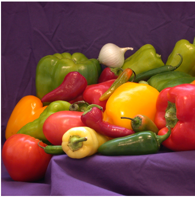
(a) True Image

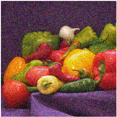
(b) Input (PSNR 15.20)

(c) $\lambda=5$ (PSNR 17.39)

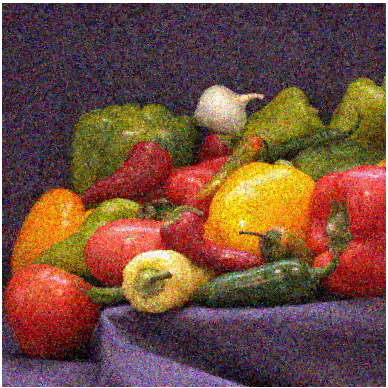
(d) $\lambda=10$ (PSNR 19.68)

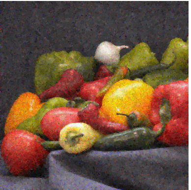
(e) $\lambda=20$ (PSNR 22.47)

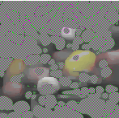
(f) $\lambda=100$ (PSNR 6.19)

Figure 1: TV-regularized denoising with increasing values of $\lambda$

For our next experiment we implemented our algorithm for a $246\times 246\times 3$ colored image, and we added some random noise to the image as before. Our experiment is illustrated in Fig. 2. The recovered images are given with different PSNR in Db and $\lambda$ values. The stopping criteria for this case are assumed to be $m_{\text{max}}=100$ and $\epsilon_{\text{tol}}=10^{-6}$. We compared our results to the Split Bregman method using the same stopping criteria. Our algorithm performed slightly better proven by the PSNR values. Split Bregman [33] is a flexible algorithm for solving non-differentiable convex minimization problems, and it is especially efficient for problems with $L_{1}$- or TV-regularization.

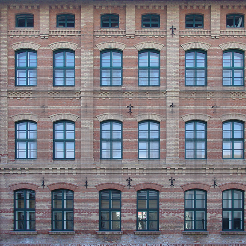
(a) True Image

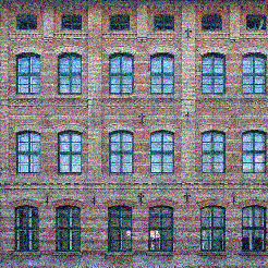
(b) Input (PSNR 18.71)

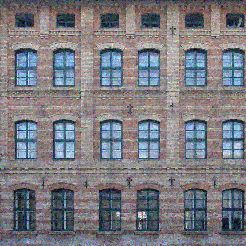
(c) Our method (PSNR 22.35)

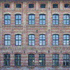
(d) Split Bregman (PSNR 19.61)

Figure 2: TV-regularized denoising with increasing values of $\lambda$.

5 Tensor Deblurring

In this section, we present a second class of TV-regularization for tensors, namely the extension of the classical deblurring problem.

Blurring always occurs in images or video recordings sometimes due to the fact that the optical system in a camera lens may be out of focus such that the incoming light is smeared out. Blurring can also occur in astronomical imaging when the light in a telescope is bent by turbulence. The goal in image deblurring is to recover the original image by using a mathematical model of the blurring process. The issue here is the lost of some hidden information present in the blurred image. Unfortunately, there is no hope of recovering the exact image due to unavoidable errors like fluctuations in the recording process and approximation errors when representing the image with a limited number of digits. In image deblurring the biggest challenge is to create an algorithm to recover as much information as possible from the given data.

The ROF-model can be extended without difficulties to the deblurring problem by replacing the fidelity term $\|f-u\|^{2}$ by $\|f-Ku\|^{2}$, where $K$ is a model for a blurring operator (e.g., a convolution operator).

Analogously, we may extend the (discretized) TV-deblurring functional to the tensor case by considering the following deblurring functional:

(16) $$\min_{\mathcal{T}\in C}\left\|\mathcal{A}(\mathcal{T})-\mathcal{S}\right\|^{2}_{F}+2\lambda TV(\mathcal{T}),$$

where $\mathcal{T}$ in $\mathbb{R}^{m\times n\times o}$ is the desired unknown image to be recovered, $\mathcal{A}$:$\mathbb{R}^{m\times n\times o}\to\mathbb{R}^{m\times n\times o}$ is a linear transformation representing some blurring operator, $\mathcal{S}$ is the observed noisy and blurred data, C is a closed convex set subset of $\mathbb{R}^{m\times n\times o}$, and $\lambda$ is the regularization parameter. TV is the discrete total variation semi-norm as above, either isotropic ($TV_{I}$) or anisotropic ($TV_{L_{1}}$). Looking at problem (16), we notice that the deblurring problem is a little more challenging than the denoising problem because of the additional blurring operator $\mathcal{A}$.

If we construct an equivalent smooth optimization algorithm for (16) via the approach in Section 4, i.e., by FISTA, we will need to invert the linear transformation matrix $\mathcal{A}$ in the proximal operator, which cannot be done by a simple threshold operator as for the denoising case.

To avoid this difficulty, we treat the TV deblurring problem (16) in two steps through the denoising problem; see, e.g., [3]. More precisely, the method iteratively solves in each step a deblurring problem with $f$ replaced by $x_{n}-\frac{2}{L}A^{*}(Ax_{n}-f)$. Thus, this approach requires at each iteration the solution of the denoising problem (9) in addition to the gradient step.

5.1 Details of the implementation

At first we focus on the blurring of 3D images. Convolving a point spread function (PSF) with a true image gives a blurred image. In our case, we assume the PSF known and given. The PSF is the function that describes the blurring and the resulting image of the point source.

Here we define convolution in N-D as follows:

$$(f*g)((n_{1},n_{2},...,n_{n})$$

$$\quad:=\sum_{j_{1}=-\infty}^{\infty}\sum_{j_{2}=-\infty}^{\infty}...\sum_{j_{n}=-\infty}^{\infty}g(j_{1},j_{2},...,j_{n})f(n_{1}-j_{1},n_{2}-j_{2},...,n_{n}-j_{n}),$$

where $f$ is our input signal (or image or video) and $g$ the kernel; it is a “filter” of the input image. If the filter is of a size smaller than the image, then we can assume that the value of the input image and kernel is 0 everywhere outside the boundary. The kernel can just be the identity kernel which is a single pixel with a value of 1, or in 2D, the kernel can be an averaging or mean filter. For instance the mean kernel for a $3\times 3$ image is a $3\times 3$ image where every entry is $\frac{1}{9}$.

For the numerical results, we are using a Gaussian filter to blur our 3D data. The PSF is a 3D gaussian function is defined as

$$\frac{1}{\sigma^{3}(2\pi)^{\frac{3}{2}}}\exp\left(-\frac{x^{2}+y^{2}+z^{2}}{2\sigma^{2}}\right).$$

To blur an image and to recover a high quality deblurred image, we must consider its boundary which is the scene outside the boundaries of an image. Ignoring the boundary can give us a reconstruction that has some artifacts at the edges. There are different types boundary conditions we can use; see [30, Ch. 4] for more details.

We will focus on the periodic boundary condition, which we extend to the N-dimensional case. For periodic boundary conditions in 2D, the PSF is a block circulant with circulant blocks (BCCB). Note that if the PSF is a BCCB matrix then it is normal and its unitary spectral decomposition is ${A}={F}^{*}\Lambda{F}$ where ${F}$ is a 2D unitary discrete Fourier Transform. We can also use this decomposition to find the eigenvalues since a circulant matrix is only defined by its first row or column; see [30]. Before going to the periodic boundary condition for tensors, we need to define the structure of a tensor and then show how we can extend the idea of circulant block to the tensor case.

A tensor $\mathcal{A}\in\mathbb{R}^{I\times J\times K}$ is called totally diagonal if $a_{ijk}$ is nonzero only if $i=j=k$. Moreover, a third order tensor $\mathcal{A}\in\mathbb{R}^{I\times J\times K}$ is called partially diagonal; i.e., diagonal in two modes or more modes for every $k$, $\mathcal{A}(i,j,k)=0,$ for $i\neq j$.

Considering a third-order tensor $\mathcal{A}\in\mathbb{R}^{n\times n\times n}$, where for every $k$, the $\mathcal{A}(:,:,k)$ slices are circulant, i.e., $\mathcal{A}(i,j,k)=\mathcal{A}(i^{\prime},j^{\prime},k)$ if $i-j\equiv i^{\prime}-j^{\prime}$ (mod $n$). Hence, $\mathcal{A}$ is circulant with respect to the first and second modes, and we then define $\mathcal{A}$ to be $\{1,2\}$-circulant.

Furthermore, a tensor $\mathcal{A}\in\mathbb{R}^{I_{1}\times...\times I_{n}}$ is called $\{l,k\}$-circulant, if $I_{l}=I_{k}=n$, and

$$\mathcal{A}(:,...,:,i_{l},...,i_{k},:,...,:)=\mathcal{A}(:,...,:,i^{\prime}_{l},...,i^{\prime}_{k},:,...,:),$$

where $i_{l}-i_{k}=i^{\prime}_{l}-i^{\prime}_{k}$ (mod $n$). Now using Eq. 20 we have that every column of the matrix $\mathcal{A}(:,:,k)$ can be constructed from $\mathcal{A}(:,1,k)$. This means that for every $j=1,...,n,$

(17) $$\mathcal{A}(:,j,k) =C^{j-1}\mathcal{A}(:,1,k)\quad\text{ and }$$

(18) $$\mathcal{A}(:,j,:) =(C^{j-1})_{1}.\mathcal{A}(:,1,:),$$

where $1$ is in the $k$th mode of $\mathcal{A}$ in Eq. 17 and the shift matrix is defined as

(19) $$C=\begin{bmatrix}0&&&1\\ 1&\ddots&&\\ &\ddots&\ddots&\\ 0&&1&0\end{bmatrix}.$$

5.2 Diagonalization of tensors with circulant structure

Here we would like to cover the case of periodic boundary condition for multidimensional matrices. For simplicity, we focus on the 3D case with an straightforward generalization to the N-dimensional case. We use periodic boundary condition because it is one of the most common boundary condition, and it has the advantage that its linear system has a circulant structure, which makes it possible to solve the problem using Fast Fourier Transform (FFT). To achieve this goal we will first define a tensor with circulant structure.

We know that a circulant matrix is entirely determined by its first column (or row); i.e., for a matrix $A$ we have

(20) $$A(:,j)=C^{j-1}a,\quad j=1,....,n\qquad\text{ and }\qquad A(i,:)=(C^{i-1}b)^{T},\quad i=1,....,n,$$

where $a$ and $b^{T}$ are the first column and row of $A$ respectively and the shift matrix $C$ is defined as in (19). Hence, any circulant matrix can be diagonalized by a Fourier matrix [32]. Note that the fact that the columns (or rows) of a circulant matrix can be written in terms of the power of the shift matrix $C$ times the first column (row), and this is what allows it to be diagonalized using the discrete Fourier transform.

Proposition 5 (Diagonalization of a circulant matrix [31]).

Let $A\in\mathbb{R}^{n\times n}$ be a circulant matrix. Then A is diagonalized by a Fourier matrix $F$ as

(21) $$\begin{split}A=F^{*}\Lambda_{1}F,\quad\Lambda_{1}=\operatorname{diag}(\sqrt{n}Fa),\\ A=F\Lambda_{2}F^{*},\quad\Lambda_{2}=\operatorname{diag}(\sqrt{n}Fb),\end{split}$$

where a and $b^{T}$ are the first column and row of A, respectively, and $\Lambda_{1}$ and $\Lambda_{2}$ are conjugate (i.e. $\Lambda_{1}=\bar{\Lambda}_{2}$).

The same idea can be used here for tensors as well. If we consider tensors whose slices are circulant with respect to a pair of modes, then we can write them in terms of powers of the shift matrix $C$, which in turn makes it possible to diagonalize the tensor using the Fourier transform. Considering shifts of slices, it is straightforward to obtain the following relations,

Lemma 5.1 (see [31]).

If $\mathcal{A}\in\mathbb{R}^{I_{1}\times\cdot\times I_{N}}$ is $\{l,k\}$-circulant, then for every $1\leq i_{k}\leq I_{k}$ we have

$$\mathcal{A}(:,\cdots,:,\cdots,i_{k},\cdots,:)=(C^{i_{k}-1})_{l}\cdot\mathcal{A}(:,\cdots,:,\cdots,1,\cdots,:),$$

and for every $1\leq i_{l}\leq I_{l}$

$$\mathcal{A}(:,\cdots,i_{l},\cdots,:,\cdots,:)=(C^{i_{l}-1})_{k}\cdot\mathcal{A}(:,\cdots,1,\cdots,:,\cdots,:),$$

where $1$ is in the $k$th and $l$th mode of $\mathcal{A}$ in the first and second equations, respectively.

Theorem 6.

Let $\mathcal{A}\in\mathbb{R}^{I_{1}\times...\times I_{6}}$ be such that for every $i=1,2,3,$ $\mathcal{A}$ is $\{i,i+3\}$-circulant. Then for every $i_{4},...,i_{2n}$,

$$\mathcal{A}(:,:,:,i_{4},...,i_{6})=(C^{i_{4}-1},...,C^{i_{6}-1})_{1,2,3}\mathcal{A}(:,:,:,1,...,1).$$

Theorem 7 (see [31]).

Let $\mathcal{A}\in\mathbb{R}^{I_{1}\times I_{2}\times I_{3}}$be $\{l,k\}$-circulant. Then $\mathcal{A}$ satisfies $\mathcal{A}=(F^{*},F)_{l,k}.\Omega$, where $\Omega$ is a $\{l,k\}$-diagonal tensor with diagonal elements $\mathcal{D}=(\sqrt{n}F)_{l}.\mathcal{A}(:,...,1,:,...,:)$; here $1$ is in the $k$th mode of $\mathcal{A}$. In particular, $\Omega(\bar{i})=\delta_{i_{l}i_{k}}\mathcal{D}(\bar{i_{k}})$, with the multi-indices $\bar{i}=(i_{1},i_{2},i_{3})$ and $\bar{i_{k}}=(i_{1},...,i_{k-1},i_{k+1},...,i_{3})$.

Theorem 8 ([31]).

Let $\mathcal{A}\in\mathbb{R}^{I_{1}\times...\times I_{6}}$ be such that for every $i=1,2,3$, $\mathcal{A}$ is $\{i,i+3\}$-circulant, and $\mathcal{X}\in\mathbb{R}^{I_{1}\times I_{2}\times I_{3}}$. The linear system of equations

(22) $$\mathcal{Y}=\langle\mathcal{A},\mathcal{X}\rangle_{1:3;1:3},$$

is equivalent to $\bar{\mathcal{Y}}=\mathcal{D}.*\bar{\mathcal{X}}$, where $\langle\mathcal{A},\mathcal{X}\rangle_{1:3;1:3}$ are the contracted product of two tensors (see [36] chapter 2),

$$\bar{\mathcal{Y}} =(F^{*},...,F^{*})_{1:N}.\mathcal{Y},\qquad\bar{\mathcal{X}}=(F^{*},...,F^{*})_{1:N}.\mathcal{X}\quad\text{ and }$$

$$\mathcal{D} =(\sqrt{I_{1}}F,...,\sqrt{I_{N}}F)_{1:N}.\mathcal{A}(:,...,:,1,...,1).$$

From the above theorems, using the periodic boundary condition, we know that the 3D case is just a generalisation of the 1D and 2D cases; see [30]. 3D or higher-dimensional cases are handled by increasing the number of modes.

If we have two third-order tensors $\mathcal{X}\in\mathbb{R}^{n\times n\times n}$ and $\mathcal{Y}\in\mathbb{R}^{n\times n\times n}$ being the true and blurred image, respectively, and $\mathcal{G}$ be the PSF array with center at $\mathcal{G}(l_{1},l_{2},l_{3})$, then the rotated PSF will be defined by $\hat{G}=(C^{l_{1}}J,C^{l_{2}}J,C^{l_{3}}J)_{1:3}.\mathcal{G}$. Furthermore, the relation between the true and blurred image can be written as tensor-tensor linear system

$$\mathcal{Y}=\langle A,\mathcal{X}\rangle_{1:3;1:3},\qquad\mathcal{A}(:,:,:,i,j,k)=(C^{i-1},C^{j-1},C^{k-1})_{1:3}.\hat{G},$$

where $\mathcal{A}$ is a $\{1,4\}$, $\{2,5\}$ and $\{3,6\}$-circulant tensor. Hence by 8 this linear system is equivalent to $\bar{\mathcal{Y}}=\bar{\mathcal{G}}.*\bar{\mathcal{X}}$, where

$$\bar{\mathcal{Y}} =(F^{*},F^{*},F^{*})_{1:3}\cdot\mathcal{Y},\qquad\bar{\mathcal{X}}=(F^{*},F^{*},F^{*})_{1:3}\cdot\mathcal{X}\quad\text{ and }$$

$$\bar{\mathcal{G}} =(\sqrt{n}F,\sqrt{n}F,F)\sqrt{n}_{1:3}\cdot\mathcal{A}(:,:,:,1,1,1)=(\sqrt{n}F,\sqrt{n}F,F)\sqrt{n}_{1:3}\cdot\mathcal{P}.$$

So, $\mathcal{Y}=\text{\text{fftn}}(\text{fftn}(\hat{G})\cdot*\text{ifft}(\mathcal{X}))$ with the discrete Fourier transform denoted as fftn and ifft its inverse. Therefore, a naive solution to the deblurring problem can be calculated by $\mathcal{X}=\text{fftn}(\text{ifft}(\mathcal{Y}\cdot/\text{fftn}(\hat{\mathcal{G}}))$. This, however, is not feasible since $\hat{\mathcal{G}}$ may have very small (or zero) values and thus cannot be inverted.

6 Numerical Experiments

All of our experiments were run using MATLAB R2016B version. Our first experiment we implemented our algorithm on a $240\times 240\times 114$video that is affected by a $15\times 15\times 3$ Gaussian blur. Also we added some random noise. The PNSR of the blurred and noisy video is 33.978db. The regularization parameter was chosen to be $\lambda=0.01$. The recovered video is given with different PSNR 37.042 Db. Our experiment is illustrated in Fig. 3. The stopping criteria for this case are assumed to be $m_{\text{max}}=100$.

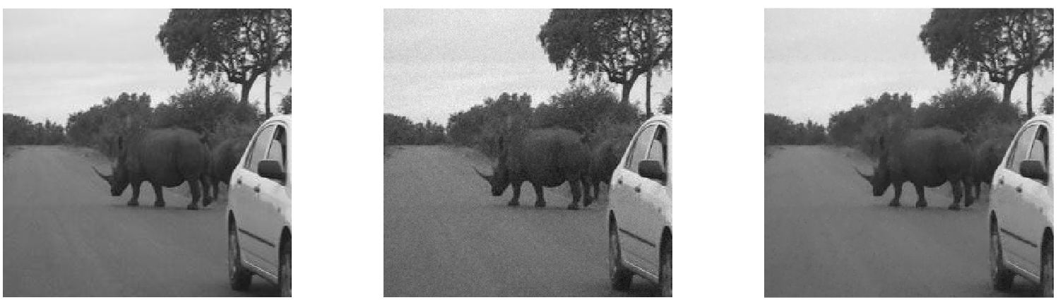
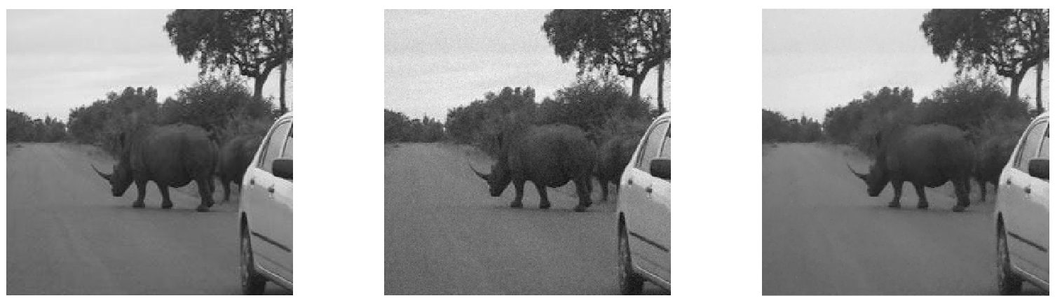
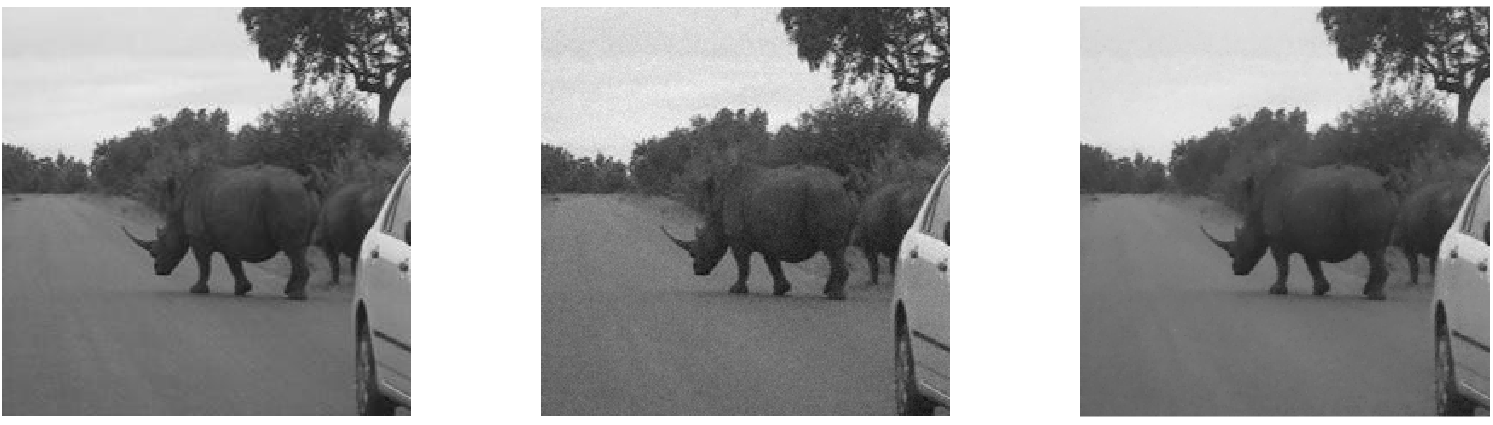
Figure 3: Three frames of the video with True image (left), Noisy input (PNSR 33.978) and recovered image (right) (PNSR 37.042) at each row.

Our second experiment we implemented our algorithm on a $200\times 200\times 3$ colored image from the MATLAB image processing toolbox. We applied a $15\times 15\times 3$ Gaussian blur and added some random noise. Note that in the experiments for Fig. 4, Fig. 5, and Fig. 6, a blurring is also applied in the color mode, which leads to a less colorful input image with ”averaged“ colors. The PNSR of the blurred and noisy image is 19.92 Db. The regularization parameter was chosen to be $\lambda=0.02$. The recovered image is given with different PSNR 22.13 Db. Our experiment is illustrated in Fig. 4. The stopping criteria for this case is $m_{\text{max}}=100$.

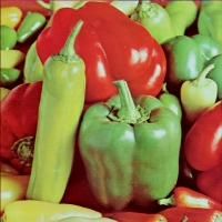
(a) True Image

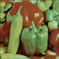
(b) Input (PSNR 19.92)

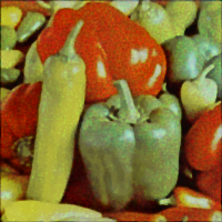
(c) Output (PSNR 22.13)

Figure 4: TV-regularized deblurring with PSNR values.

Our next experiment we implemented our algorithm on a $768\times 768\times 3$ colored image from the MATLAB image processing toolbox. We applied a $45\times 45\times 3$ Gaussian blur, again with added random noise. The PNSR of the blurred and noisy image is 20.67 Db. The regularization parameter was chosen to be $\lambda=0.01$. The recovered image is given with different PSNR 22.7 Db. Our experiment is illustrated in Fig. 5. The stopping criteria for this case is $m_{\text{max}}=150$.

(a) True Image

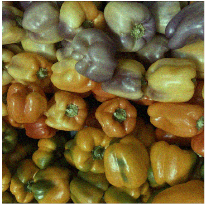
(b) Input (PSNR 20.67)

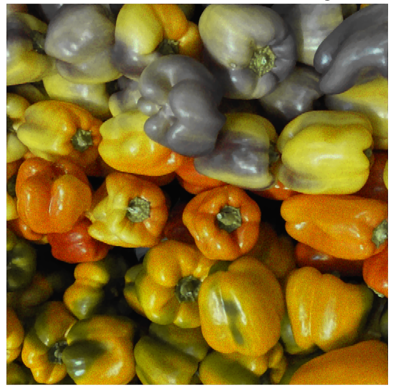
(c) Output (PSNR 22.7)

Figure 5: TV-regularized deblurring with PSNR values.

Our last experiment we implemented our algorithm on a $246\times 246\times 3$ colored image. We applied a $15\times 15\times 3$ Gaussian blur with some random noise. The PNSR of the blurred and noisy image is 19.03 Db. The regularization parameter was chosen to be $\lambda=0.02$. The recovered image is given with different PSNR 22.47 Db. Our experiment is illustrated in Fig. 6. The stopping criteria for this case is $m_{\text{max}}=150$.

(a) True Image

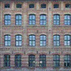
(b) Input (PSNR 19.03)

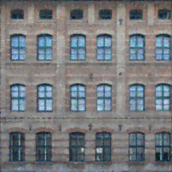
(c) Output (PSNR 22.47)

Figure 6: TV-regularized deblurring with PSNR values.

7 Conclusion

In this article we applied fast gradient-based schemes for the constrained total variation based tensor denoising and deblurring problems. The methodology is general enough to cover other types of nonsmooth regularizers. The proposed model is simple and relies on combining a dual approach with a fast gradient projection scheme as in [3]. Our numerical results show a good performance of the algorithms for the considered nonsmooth variational regularization problem for tensors.

References

- [1] A. Beck, M. Teboulle, A fast iterative shrinkage-thresholding algorithm for linear inverse problems, SIAM journal on imaging sciences, Vol. 2, no. 1, pp. 183-202 (2009).
- [2] A Beck, M Teboulle, Gradient-based algorithms with applications to signal recovery, Convex optimization in signal processing, 2009.
- [3] A. Beck and M. Teboulle, Fast Gradient-Based Algorithms for Constrained Total Variation Image Denoising and Deblurring Problems, in IEEE Transactions on Image Processing, vol. 18, no. 11, pp. 2419-2434, Nov. 2009, doi: 10.1109/TIP.2009.2028250.
- [4] L. Rudin, S. J. Osher, and E. Fatemi, Nonlinear total variation based noise removal algorithms, Physica D., 60:259–268, 1992. [also in Experimental Mathematics: Computational Issues in Nonlinear Science (Proc. Los Alamo Conf. 1991)].
- [5] A. S. Carasso, Linear and nonlinear image deblurring: A documented study, SIAM J. Numer. Anal., 36(6):1659–1689, 1999.
- [6] G. Demoment, Image reconstruction and restoration: Overview of common estimation structures and problems, IEEE Trans. Acoust., Speech, Signal Process., 37(12):2024–2036, 1989.
- [7] A. K. Katsaggelos, Digital Image Restoration, Springer-Verlag, 1991.
- [8] R. Neelamani, H. Choi, and R. G. Baraniuk, Wavelet-based deconvolution for ill-conditioned systems, In Proc. IEEE ICASSP, volume 6, pages 3241–3244, Mar. 1999.
- [9] A. Chambolle and P. L. Lions, Image recovery via total variation minimization and related problems, Numer. Math., 76(2):167–188, 1997.
- [10] L. Rudin and S. Osher, Total variation based image restoration with free local constraints, Proc. 1st IEEE ICIP, 1:31–35, 1994.
- [11] A. Chambolle, An algorithm for total variation minimization and applications, J. Math. Imag. Vis., vol. 20, no. 1–2, pp. 89–97, 2004.
- [12] A. Chambolle, Total variation minimization and a class of binary MRF models, Lecture Notes Comput. Sci., vol. 3757, pp. 136–152, 2005.
- [13] Stanley J. Osher and Selim Esedoglu, Decomposition of Images by the Anisotropic Rudin-Osher-Fatemi Model, Comm. Pure Appl. Math. 57, pp. 1609-1626, (2004).
- [14] Y. E. Nesterov, Smooth minimization of nonsmooth functions, Math. Program., 103(2005), pp. 127-152.
- [15] Y. E. Nesterov, A method for solving the convex programming problem with convergence rate O(1/k2), Dokl. Akad. Nauk SSSR, 269 (1983), pp. 543–547 (in Russian).
- [16] J. Weickert, Anisotropic Diffusion in Image Processing, vol. 1, Teubner, Stuttgart, Germany, 1998.
- [17] Boying Wu, Elisha Achieng Ogada, Jiebao Sun, Zhichang Guo, A Total Variation Model Based on the Strictly Convex Modification for Image Denoising, Abstract and Applied Analysis, vol. 2014, Article ID 948392, 16 pages, 2014. https://doi.org/10.1155/2014/948392
- [18] T. F. Chan and J. Shen, Mathematical models for local nontexture inpaintings, SIAM Journal on Applied Mathematics, vol. 62, no. 3, pp. 1019–1043, 2001.
- [19] C. R. Vogel, Total variation regularization for Ill-posed problems, Tech. Rep., Department of Mathematical Sciences, Montana State University, 1993.
- [20] L. Vese, Problemes variationnels et EDP pour lA analyse dA images et lA evolution de courbes, [Ph.D. thesis], Universite de Nice Sophia-Antipolis, 1996.
- [21] Y. Chen, S. Levine, and M. Rao, Variable exponent, linear growth functionals in image restoration, SIAM Journal on Applied Mathematics, vol. 66, no. 4, pp. 1383–1406, 2006.
- [22] T. F. Chan and S. Esedoḡlu, Aspects of total variation regularized L1 function approximation, SIAM Journal on Applied Mathematics, vol. 65, no. 5, pp. 1817–1837, 2005.
- [23] T. Chan, A. Marquina, and P. Mulet, High-order total variation-based image restoration, SIAM Journal on Scientific Computing, vol. 22, no. 2, pp. 503–516, 2000.
- [24] F. Andreu-Vaillo, V. Caselles, and J. M. Mazón, Parabolic QuasiLinear Equations Minimizing Linear Growth Functionals, vol. 223, Springer, 2004.
- [25] R. Acar and C. R. Vogel, Analysis of bounded variation penalty methods for ill-posed problems, Inverse Problems, vol. 10, no. 6, pp. 1217–1229, 1994.
- [26] D. M. Strong and T. F. Chan, Spatially and scale adaptive total variation based regularization and anisotropic diffusion in image processing, in Diusion in Image Processing, UCLA Math Department CAM Report, Cite-seer, 1996.
- [27] Carter, J.L., Dual method for total variation-based image restoration, Report 02-13, UCLA CAM (2002)
- [28] Chan, T.F., Golub, G.H., Mulet, P., A nonlinear primal-dual method for total variation based image restoration, SIAM Journal of Scientific Computing 20, 1964–1977 (1999).
- [29] Ekeland, I., Temam, Convex Analysis and Variational Problems, SIAM Classics in Applied Mathematics. SIAM (1999).
- [30] Per Christian Hansen, James G. Nagy, Dianne P. O’Leary, Deblurring Images: Matrices, Spectra and Filtering, SIAM, 2006.
- [31] Mansoor Rezghi and Lars Eldén, Diagonalization of tensors with circulant structure, Linear Algebra and its Applications, vol.435, no.3, pages 422-447,2011.
- [32] Philip J. Davis, Circulant Matrices, Division of Applied Mathematics, Brown University, JOHN WILEY & SONS, New York, 1979.
- [33] Getreuer, Pascal, Rudin-Osher-Fatemi Total Variation Denoising using Split Bregman, Image Processing On Line, vol.2, pages 74–95, 2012.
- [34] Bolei Zhou, Agata Lapedriza, Aditya Khosla, Aude Oliva, and Antonio Torralba, Places: A 10 million Image Database for Scene Recognition, IEEE Transactions on Pattern Analysis and Machine Intelligence (2017).
- [35] F. Facchinei and J. S. Pang, Finite-dimensional variational inequalities and complementarity problems, in Springer Series in Operations Research. New York: Springer-Verlag, 2003, vol. II.
- [36] S. Kobayashi, K. Nomizu, Foundations of Differential Geometry, Interscience Publisher, 1963.
- [37] R. Bruck, An iterative solution of a variational inequality for certain monotone operator in a Hilbert space, Bulletin of the American Mathematical Society, vol. 81, no. 5, pp. 890–892, 1975.
- [38] PASSTY, G. B., Ergodic Convergence to a Zero of the Surp of Monotone Operators in Hilbert Space, Journal of Mathematical Analysis and Applications 72:383-390, (1979).