On uniqueness theorems for the inverse problem of Electrocardiography in the Sobolev spaces

Abstract.

We consider a mathematical model related to reconstruction of cardiac electrical activity from ECG measurements on the body surface. An application of recent developments in solving boundary value problems for elliptic and parabolic equations in Sobolev type spaces allows us to obtain uniqueness theorems for the model. The obtained results can be used as a sound basis for creating numerical methods for non-invasive mapping of the heart.

Introduction

The inverse problem of electrocardiography, i.e. the problem of reconstruction of cardiac electrical activity from ECG measurements on the body surface is of great value for diagnostics and treatment of cardiac arrhythmias [13]. The inverse electrocardiography problem can be considered in various statements. In this paper we focused on the inverse problem of reconstruction of cardiac electrical activity inside the myocardium.

Electrophysiological processes in the myocardium are most often described using the so-called bidomain model, see [11], [19], [57] and elsewhere.

The bidomain model can be presented in the form of two non-linear parabolic partial differential equation of reaction-diffusion type or in the form of a linear elliptic equation of the second order and a non-linear reaction-diffusion equation. The reaction term of the parabolic equations characterizes transmembrane ionic currents through the potential-sensitive ion channels. It is described by a set of ordinary non-linear differential equations (also referred to as the ionic model) or, in the simplest case, a nonlinear “activation” function. The reaction term can also include an external electrical current, that allows describing the processes of electrical stimulation of the heart. The bidomain model can be complemented with the Laplace equation for the electric field potential outside the myocardium, boundary conditions on the torso surface, and interface conditions at the boundary of the myocardial domain (the bidomain-bath model).

The bidomain model was initially proposed in the late 60-70s [54], [66], [41]. Formal derivations of the model equations and the boundary conditions with different levels of mathematical rigor were obtained later [43], [29], [45], [22], [14], [21], [6]. The bidomain model is widely used for simulation the propagation of the myocardial excitation, which consists in the numerical solving the initial-boundary value problem for the corresponding equations [12], [65], [7], [48], [46]. This initial-boundary value problem was extensively studied theoretically. Positive results on the existence, uniqueness, and regularity of the ”weak” and ”strong” solution to this problem for several versions of the ”ionic model” in the framework of the suitable functional spaces were obtained in [15], [5], [10], [68], [30], [31], [44].

The bidomain model is widely accepted as an accurate model for the cardiac electrical activity [11]. Therefore, it seems reasonable to formulate the problem of reconstructing the electrical activity inside the myocardium as an inverse problem for the bidomain equations.

This problem can be attributed to the class of so-called interface problems for partial differential equations. However, such problem are expected to be essentially ill-posed unlike the classical well-posed transmission problems in the theory of elliptic boundary value problems.

In most works, only the linear elliptic equations of the bidomain–bath model were used for formulation such inverse problem [42]. Inverse problems of this class were investigated numerically in a series of works, see, for instance [24], [37], [69], [71], in which various constraints were imposed on the solution in order to obtain the uniqueness of the numerical solution and the stability of the computational procedure. The authors were able to demonstrate the feasibility of a plausible-looking reconstruction of electrical activity inside the myocardium. However, from the applied point of view, the physiological adequacy of the solution obtained by this method strongly depends on the accuracy of the a priori approximation of the solution.

In contrast to the initial-boundary value problem, the inverse problems for the bidomain mode are not sufficiently studied. Recently, theoretical investigations of the inverse problem led to interesting results about non-uniqueness and existence of its solutions in Hardy type spaces, were presented in see [25]. However, the results were obtained under the following very restrictive assumptions: all the elliptic operators involved in the model should be proportional.

Previously, Burger at al. [11] considered the possibility of solving the inverse problem for the steady (elliptic) part of the bidomain model using a priori information about the desired solution. More precisely, they formulated the inverse problem (in terms of the transmembrane potential) as a problem of minimizing the norm of the difference between the desired and a priori solution, provided that the solution satisfies the elliptic equations and the boundary conditions. The authors proved the uniqueness theorem for solving the inverse problem in this statement. This result is considered as a theoretical justification for the above-mentioned numerical methods.

The inverse problem for the complete bidomain model in the form of two reaction-diffusion equations were studied in [2]. This inverse problem provides a reconstruction of the electrical activity inside the myocardium in a special case, when the heart is activated by electrical stimulation subject to known initial conditions, for example, under the initial conditions which the myocardium has at rest. The inverse problem was stated as a problem of identification of the electrical stimulation current by known electrical potential on the body surface in the form of an optimal control problem. Using the simple two-variable Mitchell-Schaeffer ionic model, authors obtained results on the existence of the solution to this problem.

The present article is devoted to the study of the uniqueness of the solution to the problem of reconstruction of the electrical activity of the heart inside the myocardium for the bidomain model without strict restrictions (in the physiological sense) on the cardiac activation patterns. We aimed to describe conditions, providing uniqueness the theorem for both steady and evolutionary versions of the bidomain model in an essentially general situation involving both elliptic and parabolic differential operators. In this study we used a simplified linear version of the reaction term of the parabolic equation of the bidomain model. The linear assumption on the reaction part was utilized in recent papers [3], [70] for studying the inverse problem of reconstruction of electrical conductivities for the bidomain model by the Carleman estimate technique. Despite the fact that the linear activation function is a significant simplification from a physiological point of view, the results of the analysis of the linear version of the bidomain model can serve as a starting point for the study of more complex and physiologically adequate models.

In our investigation we use developments related to the ill-posed Cauchy problem for elliptic equations, see [28], [34], [62], to the Dirichlet problem and the Neumann problem for strongly elliptic operators possessing the Fredholm property, see, for instance, [20], [39], [40], [50], [55], and to the non-standard Cauchy problem for parabolic equations, see [32], [47], regarding the bidomain model as a transmission problem, see, for instance, [8] (cf. also [53] for more general models). The results of sections §2, §3 belong to V. Kalinin and A. Shlapunov, the numerical part in §4 is due to V. Kalinin and K. Ushenin.

1. Mathematical preliminaries

Let $\theta$ be a measurable set in ${\mathbb{R}}^{n}$, $n\geq 2$. Denote by $L^{2}(\theta)$ a Lebesgue space of functions on $\theta$ with the standard inner product $(\cdot,\cdot)_{L^{2}(D)}$. If $D$ is a domain in ${\mathbb{R}}^{n}$ with a piecewise smooth boundary $\partial D$, then for $s\in\mathbb{N}$ we denote by $H^{s}(D)$ the standard Sobolev space with the standard inner product $(\cdot,\cdot)_{H^{s}(D)}$. It is well-known that this scale extends for all $s>0$. More precisely, given any non-integer $s\in{\mathbb{R}}_{+}\setminus{\mathbb{Z}}_{+}$, we use the so-called Sobolev-Slobodetskii space $H^{s}(D)$, see [58].

Denote by $H^{s}_{0}(D)$ the closure of the subspace $C^{\infty}_{\mathrm{comp}}(D)$ in $H^{s}(D)$, where $C^{\infty}_{\mathrm{comp}}(D)$ is the linear space of functions with compact supports in $D$. Then the scale of Sobolev spaces can be extended for negative smoothness indexes, too. Namely, $H^{-s}(D)$ can be identified with the dual of $H^{s}_{0}(D)$ with respect to the pairing induced by $(\cdot,\cdot)_{L^{2}(D)}$.

If the boundary $\partial D$ of the domain $D$ is sufficiently smooth, then, using the standard volume form $d\sigma$ on the hypersurface $\partial D$ induced from ${\mathbb{R}}^{n}$, we may consider the Sobolev and the Sobolev-Slobodeckij spaces $H^{s}(\partial D)$ on $\partial D$.

In this section we recall both classical and recent results related to elliptic and parabolic differential operators. With this purpose, recall that a linear (matrix) differential operator

$$A(x,\partial)=\sum_{|\alpha|\leq m}A_{\alpha}(x)\partial^{\alpha}$$

of order $m$ and with $(l\times k)$-matrices $A_{\alpha}(x)$ having entries from $C^{\infty}(X)$ on an open set $X$, is called an operator with injective symbol on $X\subset{\mathbb{R}}^{n}$ if $l\geq k$ and for its principal symbol

$$\sigma(A)(x,\zeta)=\sum_{|\alpha|=m}A_{\alpha}(x)\zeta^{\alpha}$$

we have $\mathrm{rang}\,(\sigma(A)(x,\zeta))=k\mbox{ for any }x\in X,\zeta\in{\mathbb{R}}^{n}\setminus\{0\}.$ An operator $A$ is called (Petrovsky) elliptic, if $l=k$ and its symbol is injective.

An operator $L(x,\partial)$ is called strongly elliptic if it is elliptic, its order $2m$ is even and there is a positive constant $c_{0}$ such that

$$(-1)^{m}\Re{\,(w^{*}\sigma(L)}(x,\zeta)\,w)\geq c_{0}|\zeta|^{2m}|w|^{2}\mbox{ for any }x\in X,\zeta\in{\mathbb{R}}^{n},w\in{\mathbb{C}}^{k}$$

where $w^{*}=\overline{w}^{T}$ and $w^{T}$ is the transposed vector for $w\in{\mathbb{C}}^{k}$.

Denote by $\nabla$ the gradient operator and by ${\rm div}$ the divergence operator in ${\mathbb{R}}^{n}$. Obviously, the principal symbol of the operator $\nabla$ is injective. Let $M(x)$ be a $(n\times n)$ symmetric non-degenerate matrix with smooth real entries, such that there is a constant $c_{0}$ providing

(1.1) $$\zeta\cdot M(x)\zeta=\zeta^{T}M(x)\zeta\geq c_{0}|\zeta|^{2}\mbox{ for each }\zeta\in{\mathbb{R}}^{n}\setminus\{0\}\mbox{ and each }x\in\overline{X}.$$

Then the differential operator

$$-\Delta_{M}=-\mbox{div}M\nabla=-\nabla\cdot M\nabla$$

is elliptic and strongly elliptic on $X$ with $\sigma(\Delta_{M})(x,\zeta)=-\zeta\cdot M(x)\zeta$.

Next, we need suitable boundary operators.

Definition 1.1.

A set of linear differential operators $\{B_{0},B_{1},\dots B_{m-1}\}$ is called a $(k\times k)$ Dirichlet system of order $(m-1)$ on $\partial D$ if 1) the operators are defined in a neighbourhood of $\partial D$; 2) the order of the differential operator $B_{j}$ equals to $j$; 3) the map $\sigma(B_{j})(x,\nu(x)):{\mathbb{C}}^{k}\to{\mathbb{C}}^{k}$ is bijective for each $x\in\partial D$, where $\nu(x)$ will denote the outward normal vector to the hypersurface $\partial D$ at the point $x\in\partial D$.

The simplest Dirichlet pair is the pair $\{1,\frac{\partial}{\partial\nu}\}$, where $\frac{\partial}{\partial\nu}$ is the normal derivative with respect to $\partial D$. If we denote by $\partial_{\nu,M}$ the so-called co-normal derivative with respect to $\Delta_{M}$ and set $\partial_{\nu,M}=\nu^{T}M\nabla$ then $\{1,\partial_{\nu,M}\}$ is also a Dirichlet pair, under assumption (1.1).

According to the Trace Theorem, see for instance [36, Ch. 1, § 8] and [39], if $\partial D\in C^{s}$, $s\geq m\geq 1$ then for each $s\in\mathbb{N}$, $s\geq 2$, each operator $B_{j}$ induces a bounded linear operator

$$B_{j}:H^{s}(D)\to H^{s-j/2}(\partial D).$$

Thus, the Dirichlet systems are widely used to formulate boundary value problems.

Now let us discuss the Existence and Uniqueness Theorems for four boundary value problems that are essential for our approach to the models of the Electrocardiography, considered in the next sections.

We begin with the Dirichlet Problem related to strongly elliptic operators.

Problem 1.2.

Given pair $g\in H^{s-2m}(D)$ and $\oplus_{j=0}^{m-1}u_{j}\in\oplus_{j=0}^{m-1}H^{s-j-1/2}(\partial D)$ find, if possible, a function $u\in H^{s}(D)$ such that

(1.2) $$\left\{\begin{array}[]{lll}Lu=g&{\rm in}&D,\\ \oplus_{j=0}^{m-1}B_{j}u=\oplus_{j=0}^{m-1}u_{j}&{\rm on}&\partial D.\\ \end{array}\right.$$

The problem can be treated in the framework of operator theory in Banach spaces, regarding (1.2) as operator equation with the linear bounded operator

$$(L,\oplus_{j=0}^{m-1}B_{j}):H^{s}(D)\to H^{s-2m}(D)\times\oplus_{j=0}^{m-1}H^{s-j-1/2}(\partial D),\,s\geq m.$$

Recall that a problem related to operator equation $Ru=f$ with a linear bounded operator $R:X_{1}\to X_{2}$ in Banach spaces $X_{1},X_{2}$ has the Fredholm property, if the kernel ${\rm ker}(R)$ of the operator $R$ and the co-kernel ${\rm coker}(R)$ (i.e. the kernel ${\rm ker}(R^{*})$ of its adjoint operator $R^{*}:X_{2}^{*}\to X_{1}^{*}$) are finite-dimensional vector spaces and the range of the operator $R$ is closed in $X_{2}$.

Theorem 1.3.

Let $L$ be a strongly elliptic differential operator of order $2m$, $m\geq 1$, with smooth coefficients in a neighbourhood $X$ of $\overline{D}$, $\partial D\in C^{s}$, $s\geq m$ and $B=\{B_{0},B_{1},\dots,B_{m-1}\}$ be a Dirichlet system of order $(m-1)$ on $\partial D$. Then Problem 1.2 has the Fredholm property. Moreover if $L$ is formally non-negative and has real analytic coefficients a neighbourhood $X$ of $\overline{D}$, then Problem 1.2 has one and only one solution.

Proof.

See, for instance, [40], [50, Ch. 5] or elsewhere. ∎

Corollary 1.4.

Let $\partial D\in C^{s}$, $s\geq 1$ and let $M(x)$ be a $(n\times n)$ symmetric non-degenerate matrix with smooth real entries satisfying (1.1). Then for each pair $g\in H^{s-2}(D)$ and $u_{0}\in H^{s-1/2}(\partial D)$ there is unique function $u\in H^{s}(D)$ such that

$$\left\{\begin{array}[]{lll}\Delta_{M}u=g&{\rm in}&D,\\ u=u_{0}&{\rm on}&\partial D.\\ \end{array}\right.$$

Now we recall the Existence and Uniqueness Theorem for the interior Neumann Problem related to $\Delta_{M}$.

Problem 1.5.

Given pair $g\in H^{s-2}(D)$ and $u_{1}\in H^{s-3/2}(\partial D)$, find, if possible, a function $u\in H^{s}(D)$ such that

$$\left\{\begin{array}[]{lll}\Delta_{M}u=g&{\rm in}&D,\\ \partial_{\nu,M}u=u_{1}&{\rm on}&\partial D.\\ \end{array}\right.$$

Theorem 1.6.

Let $s\in\mathbb{N}$, $s\geq 2$, $\partial D\in C^{s}$ and let $M(x)$ be a $(n\times n)$ symmetric non-degenerate matrix with smooth real entries satisfying (1.1). Then Neumann Problem 1.5 is solvable if and only if

(1.3) $$\int_{\partial D}u_{1}d\sigma+\int_{D}gdx=0.$$

The null-space of Problem 1.5 consists of all the constants. Moreover, under (1.3) there is only one solution $u$ satisfying

(1.4) $$\int_{\partial D}u(x)d\sigma(x)=0.$$

Proof.

See, for instance, [55]. ∎

The unique solution to Problem 1.5 satisfying (1.4) will be denoted by ${\mathcal{N}}_{i}(g,u_{1})$.

We continue the section with the discussion of the ill-posed Cauchy problem for the operator $\Delta_{M}$.

Problem 1.7.

Fix a part $S$ of $\partial D$ and a Dirichlet pair $B=\{B_{0},B_{1}\}$ on $\partial D$. Given triple $g\in H^{s-2}(D)$, $u_{0}\in H^{s-1/2}(\partial D)$ and $u_{1}\in H^{s-3/2}(\partial D)$, find, if possible, a function $u\in H^{s}(D)$ such that

$$\left\{\begin{array}[]{lll}\Delta_{M}u=g&{\rm in}&D,\\ B_{0}u=u_{0}&\rm{on}&S,\\ B_{1}u=u_{1}&\rm{on}&S.\\ \end{array}\right.$$

As the Cauchy problem is generally ill-posed, the description of its solvability conditions is rather complicated. It appears that the regularization methods (see, for instance, [64]) are most effective for studying the problem. However, there are many different ways to realize the regularization, see, for instance, [34] [38], [28] for the Cauchy problem related to the second order elliptic equations. We follow idea of the book [62], that gives a rather full description of solvability conditions for the homogeneous elliptic equations, combined with the recent results [17] for elliptic complexes. In order to formulate it we need the following Green formula.

Lemma 1.8.

Let $m\in\mathbb{N}$, $Q$ be an elliptic operator of order $(m-1)$ in a neighbourhood of $\overline{D}$ and $B=\{B_{0},B_{1},\dots B_{m-1}\}$ be a Dirichlet system of order $(m-1)$ on $\partial D$. Then there is a Dirichlet system $\tilde{B}=\{\tilde{B}_{0},\tilde{B}_{1},\dots\tilde{B}_{m-1}\}$ on $\partial D$ such that for all $v\in H^{m}(D)$, $u\in H^{m}(D)$ we have

(1.5) $$\int_{\partial D}\Big{(}\sum_{j=0}^{m-1}({\tilde{B}}_{m-1-j}v)^{*}B_{j}u\Big{)}d\sigma=\int_{D}\Big{(}v^{*}Qu-(Qv)^{*}u\Big{)}dx.$$

Proof.

See, for instance, [61, Lemma 8.3.3]. ∎

Ostrogradsky-Gauss formula yields that for $Q=\Delta_{M}$ and the Dirichlet pair $B=\{B_{0}=1,B_{1}=\partial_{\nu M}\}$ we have the dual Dirichlet pair $\tilde{B}=\{\tilde{B}_{0}=1,\tilde{B}_{1}=\partial_{\nu M}\}$.

Next, if we assume that the matrix $M$ has real analytic entries and satisfies (1.1) we note that all the solutions $u$ to equation $\Delta_{M}w=0$ in an open set $U\subset{\mathbb{R}}^{n}$ are real analytic there. Hence it admits a bilateral (left and right) fundamental solution $\varphi_{M}(x,y)$, see, for instance, [60, §2.3]. In particular, the following Green formula holds true: for each $u\in H^{2}(D)$ we have

$$\chi_{D}u={\mathcal{G}}^{(B)}_{M,\partial D}(B_{0}u,B_{1}u)+T_{M,D}(\Delta_{M}u),$$

where $\chi_{D}$ is the characteristic function of the (bounded) domain $D$ in ${\mathbb{R}}^{n}$,

$$T_{D,M}(g)(x)=\int_{D}\varphi_{M}(x,y)g(y)dy,$$

$${\mathcal{G}}^{(B)}_{M,S}(u_{0},u_{1})=\int_{S}\Big{(}u_{0}(y)\tilde{B}_{1}(y)\varphi_{M}(x,y)-u_{1}(y)\tilde{B}_{0}(y)\varphi_{M}(x,y)\Big{)}d\sigma(y)$$

with a hypersurface $S$ and $x\not\in S$.

Let us formulate a solvability criterion for Problem 1.7 under reasonable assumptions on $S$. Namely, let us assume that $S$ is a relatively open subset of $\partial D$ with a smooth boundary $\partial S$. Then for each pair $u_{0}\in H^{s-1/2}(S)$, $u_{1}\in H^{s-3/2}(S)$ there are functions $\tilde{u}_{0}\in H^{s-1/2}(\partial D)$, $u_{1}\in H^{s-3/2}(S)$, such that $\tilde{u}_{0}=u_{0}$, $\tilde{u}_{1}=u_{1}$ on $S$.

Let us fix a domain $D^{+}$ such that $D\cap D^{+}=\emptyset$ and the set $G=D\cup S\cup D^{+}$ is a piece-wise smooth domain. We denote by $({\mathcal{G}}^{(B)}_{M,\partial D}(u_{0},u_{1}))^{+}$ the restriction of the potential ${\mathcal{G}}^{(B)}_{M,\partial D}(u_{0},u_{1})$ onto $D^{+}$ and similarly for the potential $T_{M,D}(g)$. Obviously,

$$\Delta_{M}({\mathcal{G}}^{(B)}_{M,\partial D}(u_{0},u_{1}))^{+}=\Delta_{M}(T_{M,D}(g))^{+}=0\mbox{ in }D^{+}$$

as a parameter dependent integral.

Theorem 1.9.

Let $s\in\mathbb{N}$, $s\geq 2$, $\partial D\in C^{s}$ and the matrix $M$ have real analytic entries and satisfy (1.1). If $\partial D\setminus S$ has at least one interior point in the relative topology then Problem 1.7 is densely solvable. If $S$ is a relatively open subset of $\partial D$ with a smooth boundary $\partial S$ then Cauchy Problem 1.7 has no more than one solution. It is solvable if and only if there is a function ${\mathcal{F}}\in H^{s}(G)$ satisfying $\Delta_{M}{\mathcal{F}}=0$ in $G$ and such that

$${\mathcal{F}}=({\mathcal{G}}^{(B)}_{M,\partial D}(\tilde{u}_{0},\tilde{u}_{1}))^{+}+(T_{M,D}g)^{+}\mbox{ in }D^{+}.$$

Besides, the solution $u$, if exists, is given by the following formula

(1.6) $$u={\mathcal{G}}^{(B)}_{M,\partial D}(\tilde{u}_{0},\tilde{u}_{1})+T_{M,D}g-{\mathcal{F}}\mbox{ in }D.$$

Proof.

See, for instance, [52, Theorems 2.8 and 5.2] for the case $g=0$ and [17] for $g\neq 0$. ∎

At the end of the section we give some information about parabolic theory. With this purpose, let $\Omega_{T}$ be the cylinder domain $\Omega\times(0,T)$ with the base $\Omega$ and the time interval $(0,T)$. Let us denote by $H^{2s,s}(\Omega_{T})$, $s\in{\mathbb{Z}}_{+}$, anisotropic (parabolic) Sobolev spaces, see, for instance, [33], i.e. the set of such measurable functions $u$ on $\Omega_{T}$ that the partial derivatives $\partial^{j}_{t}\partial^{\alpha}_{x}u$ belong to the Lebesgue space $L^{2}(\Omega_{T})$ for all multi-indexes $(\alpha,j)\in{\mathbb{Z}}_{+}^{n}\times{\mathbb{Z}}_{+}$ satisfying $|\alpha|+2j\leq 2s$. This is a Hilbert space with the natural inner product $(u,v)_{H^{2s,s}(\Omega_{T})}$.

We will also use the so-called Bochner spaces of functions depending on $(x,t)$ over $\Omega_{T}$. Namely, if $\mathcal{B}$ is a Banach space (possibly, a space of functions over $\Omega$) and $p\geq 1$, we denote by $L^{p}([0,T],{\mathcal{B}})$ the Banach space of measurable maps $u:[0,T]\to{\mathcal{B}}$ with the standard norm, see, for instance, [35, Ch. §1.2].

Similarly to elliptic theory, one use often integral representations in parabolic theory, too. Consider the differential operator ${\mathcal{L}}_{M}=\partial_{t}+\Delta_{M}$ and a more general differential operator

$${\mathcal{L}}={\mathcal{L}}_{M}+\sum_{j=1}^{n}a_{j}(x)\partial_{j}+a_{0}(x)$$

with variable coefficients $a_{j}(x)$, $0\leq j\leq n$. As the operator $\Delta_{M}$ is strongly elliptic then the operator ${\mathcal{L}}$ is parabolic, see, for instance, [40], [18]. In the particular case $M=I$, we obtain the heat operator ${\mathcal{L}}_{M}=\partial_{t}-\Delta$.

Under rather mild assumptions on the coefficients $M$ and $a_{j}$, $0\leq j\leq n$, the parabolic differential operator ${\mathcal{L}}$ admits a fundamental solution $\Psi_{\mathcal{L}}$. In particular, it is the case if the coefficients are constant or real analytic and bounded at the infinity, see, for instance, [16, §1.5, Theorem 2.8] or [18, Ch.1, §1–5].

Example 1.10.

Let $M$ be a non-degenerate matrix with real constant entries. If we denote by $M^{-1}$ the inverse matrix for $M$ then the kernel

$$\Psi_{{\mathcal{L}}_{M}}(x,y,t,\tau)=\begin{cases}\frac{e^{-\frac{(x-y)^{T}M^{-1}(x-y)}{4(t-\tau)}}}{\left(2\sqrt{\pi{\rm det}(M)\,(t-\tau)}\right)^{n}}&\mbox{ if }t>\tau,\\ 0&\mbox{ if }t\leqslant\tau,\end{cases}$$

is the the fundamental solution to the operator ${\mathcal{L}}_{M}$, see [18, Ch.1, §2].

Assume that the the parabolic differential operator ${\mathcal{L}}$ admits a fundamental solution $\Psi_{\mathcal{L}}$. Denote by $S$ a relatively open subset of $\partial\Omega$ and set $S_{T}=S\times(0,T)$. For functions $g\in L^{2}(\Omega_{T})$, $w\in L^{2}([0,T],H^{3/2}(\partial\Omega))$, $v\in L^{2}([0,T],H^{1/2}(\partial\Omega))$, $h\in H^{1/2}(\Omega)$ we introduce the following potentials:

$$I_{\Omega}(h)(x,t)=\int\limits_{\Omega}\Psi_{\mathcal{L}}(x,y,t,0)h(y)dy,$$

(1.7) $$G_{\Omega}(f)(x,t)=\int\limits_{0}^{t}\int\limits_{\Omega}\Psi_{\mathcal{L}}(x,y,\ t,\tau)g(y,\tau)dyd\tau,$$

$$V_{S}(v)(x,t)=\int\limits_{0}^{t}\int\limits_{S}\tilde{B}_{0}(y)\Psi_{\mathcal{L}}(x,y,t,\tau)v(y,\tau)ds(y)d\tau,$$

$$W_{S}(w)(x,t)=-\int\limits_{0}^{t}\int\limits_{S}\tilde{B}_{1}(y)\Psi_{\mathcal{L}}(x,y,t,\tau)w(y,\tau)ds(y)d\tau,$$

(see, for instance, [18, Ch. 1, §3 and Ch. 5, §2]), [59, Ch. 6, §12]m where $\tilde{B}=(\tilde{B}_{0},\tilde{B}_{1})$ is the dual Dirichlet pair for the elliptic operator

$$\Delta_{M}+\sum_{j=1}^{n}a_{j}\partial_{j}+a_{0}$$

and the Dirichlet pair $B=(1,\partial_{\nu,M})$, see Lemma 1.8. The potential $I_{\Omega}(h)$ is sometimes called Poisson type integral and the functions $G_{\Omega}(g)$, $V_{S}(v)$, $W_{S}(w)$ are often referred to as heat potentials or, more precisely, Volume Parabolic Potential, Single Layer Parabolic Potential and Double Layer Parabolic Potential, respectively. By the construction, all these potentials are (improper) integral depending on the parameters $(x,t)$.

The theory of boundary value problem for parabolic operators in cylinder domains are closely related to the elliptic theory. However, we consider a non-standard Cauchy problem for parabolic operators in cylinder domain $\Omega_{T}$ with the Cauchy data on its lateral surface $\partial\Omega\times[0,T]$, see, for instance, [47], [32].

Problem 1.11.

Given $u_{1}\in L^{2}([0,T],H^{3/2}(S))$, $u_{2}\in L^{2}([0,T],H^{1/2}(S))$, $g\in L^{2}(\Omega_{T})$, find $u\in H^{2,1}(\Omega_{T})$, satisfying

$$\left\{\begin{array}[]{lll}{\mathcal{L}}u=g&{\rm in}&\Omega_{T},\\ u=u_{1}&{\rm on}&S_{T},\\ \partial_{\nu,M}u=u_{2}&{\rm on}&S_{T}.\\ \end{array}\right.$$

This problem is generally ill-posed. It may be treated similarly to the ill-posed Cauchy problem for elliptic equations, [32], [47]. Let us fix a domain $\Omega^{+}$ such that $\Omega\cap\Omega^{+}=\emptyset$ and the set $D=\Omega\cup S\cup\Omega^{+}$ is a piece-wise smooth domain. We denote by $(I_{\Omega}(u))^{+}$ the restriction of the potential $I_{\Omega}(u)$ onto $\Omega^{+}$ and similarly for the potentials $W_{S}(w)$, $V_{S}(v)$ and $G_{\Omega}(f)$. Obviously,

$${\mathcal{L}}(I_{\Omega}(u))^{+}={\mathcal{L}}(G_{\Omega}(f))^{+}={\mathcal{L}}(V_{S}(v))^{+}={\mathcal{L}}(W_{S}(w))^{+}=0\mbox{ in }(\Omega^{+})_{T}$$

as a parameter dependent integrals.

Theorem 1.12.

Let $s\in\mathbb{N}$, $s\geq 2$, and $\partial\Omega\in C^{s}$. If $S$ is a relatively open subset of $\partial\Omega$ with a smooth boundary $\partial S$ then Cauchy Problem 1.11 has no more than one solution. It is solvable if and only if there is a function ${\mathcal{F}}\in H^{2,1}(D_{T})$ satisfying ${\mathcal{L}}{\mathcal{F}}=0$ in $D_{T}$ and such that

$${\mathcal{F}}=(G_{\Omega}(f))^{+}+(W_{S}(u_{1}))^{+}+(V_{S}(u_{2}))^{+}\mbox{ in }(\Omega^{+})_{T}.$$

Besides, the solution $u$, if exists, is given by the following formula

$$u=G_{\Omega}(f)+W_{S}(u_{1})+V_{S}(u_{2})-{\mathcal{F}}\mbox{ in }D_{T}.$$

Proof.

See, for instance, [32], [47] for similar problems related to various parabolic differential operators in the anisotropic Hölder spaces and Sobolev spaces. ∎

2. A steady bidomain model of the heart

Following a standard scheme (see, for instance, [19], [57, §2.2.2], or elsewhere) let us consider the myocardial domain $\Omega_{m}$ being surrounded by a volume conductor $\Omega_{b}$. The total domain, including the myocardium and the torso $\Omega=\Omega_{b}\cup\overline{\Omega}_{m}$, where $\overline{\Omega}_{m}$ is the closure of heart domain, is surrounded by a non-conductive medium (air). We assume that the conductivity matrices $M_{i}$, $M_{e}$, $M_{b}$ of the intra-, extracellular and extracardiac media satisfy (1.1) and that their entries are real analytic in some neighbourhoods of $\overline{\Omega}_{m}$ and $\overline{\Omega}_{b}$, respectively; of course, if we assume that these media are homogeneous and isotropic, then the entries will be just constants.

Then the differential operators

$$\Delta_{e}=-\nabla\cdot M_{e}\nabla,\,\Delta_{i}=-\nabla\cdot M_{i}\nabla,\,\Delta_{b}=-\nabla\cdot M_{b}\nabla$$

are elliptic and strongly elliptic and admit the bilateral fundamental solutions, say, $\varphi_{i}$, $\varphi_{e}$, $\varphi_{b}$, over some neighbourhoods of $\overline{\Omega}_{m}$ and $\overline{\Omega}_{b}$, respectively.

If $u_{i},u_{e}\in H^{2}(\Omega_{m})$, $u_{b}\in H^{2}(\Omega_{b})$ are intra-, extracellular and extracardiac potentials, respectively, then the intra-, extracellular and extracardiac currents are given by

$$J_{i}=-M_{i}\nabla u_{i},\,J_{e}=-M_{e}\nabla u_{e},\,u_{b}=-M_{b}\nabla u_{b},$$

respectively. As the intracellular charge $q_{i}$ and the extracellular $q_{e}$ should be balanced in the heart tissue, we arrive at the following equations

(2.1) $$\frac{\partial(q_{i}+q_{e})}{\partial t}=0,$$

(2.2) $$-\Delta_{i}u_{i}=\frac{\partial q_{i}}{\partial t}+\chi I_{\rm ion},$$

(2.3) $$-\Delta_{e}u_{e}=\frac{\partial q_{e}}{\partial t}-\chi I_{\rm ion},$$

where $I_{\rm ion}$ is the ionic current across the membrane and $\chi I_{\rm ion}$ is ionic current per unit tissue. Of course, the potentials $u_{e}$ and $u_{i}$ are actually defined on different domains: extracellular and intracellular spaces in $\Omega_{m}$, respectively. Thus, the last equations reflect the fact that a homogenization procedure is at the bottom of the bidomain model.

Then, combining (2.1), (2.3) (2.2) we obtain the conservation law for the total current $(J_{i}+J_{e})$:

$$\Delta_{i}u_{i}+\Delta_{e}u_{e}=0\mbox{ in }\Omega_{m}.$$

Next, denote by $\nu_{i}$, $\nu_{e}$ the outward normal vectors to the surfaces of the heart and body volume ($\Omega_{m}$ and $\Omega_{b}$), respectively. In the heart surrounded by a conductor, the normal component of the total current should be continuous across the boundary of the heart:

(2.4) $$\nu_{i}\cdot(J_{i}+J_{e})=\nu_{i}\cdot J_{b}.$$

Taking in account the current behaviour at the torso, we arrive at a steady-state version of the bidomain model [19]:

(2.5) $$\Delta_{i}u_{i}+\Delta_{e}u_{e}=0\mbox{ in }\Omega_{m},$$

(2.6) $$\Delta_{b}u_{b}=0\mbox{ in }\Omega_{b},$$

(2.7) $$u_{e}=u_{b}\mbox{ on }\partial\Omega_{m},$$

(2.8) $$\nu_{i}\cdot(M_{e}\nabla u_{e})=-\nu_{e}\cdot(M_{b}\nabla u_{b})\mbox{ on }\partial\Omega_{m}$$

(2.9) $$\nu_{i}\cdot(M_{i}\nabla u_{i})=0\mbox{ on }\partial\Omega_{m},$$

(2.10) $$\nu_{e}\cdot(M_{b}\nabla u_{b})=0\mbox{ on }\partial\Omega,$$

where (2.8), (2.9) are consequences of (2.4) and the assumption that the intracellular domain is completely insulated.

However, this steady model is often supplemented by an evolutionary part. For example, (2.2), (2.3) imply

$$-\Delta_{i}u_{i}+\Delta_{e}u_{e}=\frac{\partial(q_{i}-q_{e})}{\partial t}+2\chi I_{\rm ion}.$$

On the other hand, the transmembrane potenitial $v=u_{i}-u_{e}$ satisfies

$$u_{i}-u_{e}=\frac{1}{2}\frac{q_{i}-q_{e}}{\chi\,C_{m}}$$

where $C_{m}$ is the capacitance of the cell membrane. Thus, using the last two identities we arrive at the so-called cable equation

(2.11) $$\frac{1}{2\chi}\Big{(}-\Delta_{i}u_{i}+\Delta_{e}u_{e}\Big{)}=C_{m}\frac{\partial(u_{i}-u_{e})}{\partial t}+I_{\rm ion}\mbox{ in }\Omega_{m}\times(0,T),$$

see, for instance, [57, §2.2.2]. There are other advanced and complicated relations that can be added to the model.

In this section we will discuss the steady part of the bidomain model only, considering the following problem:

Problem 2.1.

Let the values of electrical potential $u_{b}$ on the boundary of the body domain be known:

(2.12) $$u_{b}=f\mbox{ on }\partial\Omega,$$

where $f\in H^{3/2}(\partial\Omega)$. Under these conditions we seek for the intracellular potential $u_{i}\in H^{2}(\Omega_{m})$ and extracellular potential $u_{e}\in H^{2}(\Omega_{m})$ and extracardiac potential $u_{b}\in H^{2}(\Omega_{b})$ satisfying equations (2.5), (2.6) and boundary conditions (2.7)-(2.10).

The non-uniqueness of solutions to Problem 2.1 was established in [25] in specially constructed Hardy type spaces under the following restrictive assumptions:

1) all the media are homogeneous and isotropic;

2) the matrices $M_{i}$, $M_{e}$, are proportional, i.e.

(2.13) $$M_{e}=\lambda M_{i}\mbox{ with some positive number }\lambda.$$

In particular, this means that a linear change of variables reduces the consideration to the situation where

(2.14) $$\Delta_{i}=-\sigma_{i}\Delta,\,\Delta_{e}=-\sigma_{e}\Delta,\,\lambda=\frac{\sigma_{e}}{\sigma_{i}}$$

and $\sigma_{i}$, $\sigma_{e}$, are positive numbers characterizing the electrical conductivity of the corresponding media.

Let us describe the null-space of Problem 2.1 in a more general situation. With this purpose, we use the following calibration assumption that always is achievable for isotropic conductivity: there is a constant $c_{0}$ such that

(2.15) $$\int_{\partial\Omega_{m}}(u_{i}+c_{0}u_{e})(y)d\sigma(y)=0.$$

Proposition 2.2.

The null-space of Problem 2.1 consists of all the triples $u_{i},u_{e}\in H^{2}(\Omega_{m})$, $u_{b}\in H^{2}(\Omega_{b})$ satisfying the following conditions:

(2.16) $$\left\{\begin{array}[]{ccccc}u_{b}&=&0&{\rm in}&\Omega_{b},\\ u_{e}&=&u&{\rm in}&\Omega_{m},\\ u_{i}&=-&{\mathcal{N}}_{i}(\Delta_{e}u,0)+c&{\rm in}&\Omega_{m},\\ \end{array}\right.$$

where ${\mathcal{N}}_{i}$ is the Neumann operator related to $\Delta_{i}$, $c$ is an arbitrary constant and $u$ is an arbitrary function from $H^{2}_{0}(\Omega_{m})$. If calibration assumption (2.15) holds for a pair $u_{i}$, $u_{e}$ from the null-space then the constant $c$ in (2.16) equals to zero.

Proof.

Indeed, let the triple $(u_{b},u_{i},u_{e})\in H^{2}(\Omega_{b})\times H^{2}(\Omega_{m})\times H^{2}(\Omega_{m})$ belong to the null-space of Problem 2.1. Hence $f\equiv 0$ on $\partial\Omega$ and then $u_{b}\equiv 0$ in $\Omega_{b}$ because of Theorem 1.9 for the Cauchy problem. Of course, using (2.7), (2.8), we obtain

$$u_{e}=u_{b}=\nu_{i}\cdot(M_{e}\nabla u_{e})=-\nu_{e}\cdot(M_{b}\nabla u_{b})=0\mbox{ on }\partial\Omega_{m}$$

for $u_{e}\in H^{2}(\Omega_{m})$. Then, according to [23], $u_{e}\in H^{2}_{0}(\Omega_{m})$. The function $u_{i}$ satisfies (2.5) and (2.9) and then, according to Theorem 1.6, this means precisely

$$u_{i}=-{\mathcal{N}}_{i}(\Delta_{e}u_{e},0)+c$$

with an arbitrary constant $c$.

Thus, any triple $(u_{b},u_{i},u_{e})\in H^{2}(\Omega_{b})\times H^{2}(\Omega_{m})\times H^{2}(\Omega_{m})$, belonging to the null-space of Problem 2.1, has the form as in (2.16) with a constant $c$ and a function $u=u_{e}\in H^{2}_{0}(\Omega_{m})$.

Let a triple $(u_{b},u_{i},u_{e})\in H^{2}(\Omega_{b})\times H^{2}(\Omega_{m})\times H^{2}(\Omega_{m})$ have the form as in (2.16) with an arbitrary constant $c$ and an arbitrary function $u\in H^{2}_{0}(\Omega_{m})$.

Then, obviously, $f\equiv 0$ on $\partial\Omega$. Moreover, using Green formula (1.5), we easily obtain

$$-\int_{\Omega_{m}}\Delta_{e}udy=\int_{\partial\Omega_{m}}1\,\nu_{e}\cdot M_{e}\nabla ud\sigma=0$$

because $u\in H^{2}_{0}(\Omega_{m})$. Hence Theorem 1.6 implies that there is a potential $w$ satisfying Neumann Problem 1.5 for the operator $\Delta_{i}$:

$$\left\{\begin{array}[]{lll}\Delta_{i}w=-\Delta_{e}u&{\rm in}&\Omega_{m},\\ \nu_{i}\cdot M_{i}\nabla w=0&{\rm on}&\partial\Omega_{m}.\\ \end{array}\right.$$

According to Theorem 1.6, the general form of such a solution is precisely

(2.17) $$u_{i}=-{\mathcal{N}}_{i}(\Delta_{e}u_{e},0)+c$$

with a constant $c$.

If we take $u_{i}=w$ then

$$\left\{\begin{array}[]{ccccc}u_{b}&=&0&{\rm in}&\Omega_{b},\\ u_{e}&=&u&{\rm in}&\Omega_{m},\\ \nu_{i}\cdot(M_{e}\nabla u_{e})&=&0&{\rm on}&\partial\Omega_{m},\\ u_{b}&=&0&{\rm on}&\partial\Omega_{m},\\ \Delta_{i}u_{i}&=&-\Delta_{e}u&{\rm in}&\Omega_{m},\\ \nu_{i}\cdot(M_{i}\nabla u_{i})&=&0&{\rm on}&\partial\Omega_{m}.\\ \end{array}\right.$$

Thus, any triple $(u_{b},u_{i},u_{e})\in H^{2}(\Omega_{b})\times H^{2}(\Omega_{m})\times H^{2}(\Omega_{m})$ having the form as in (2.16) with a arbitrary constant $c$ and an arbitrary function $u\in H^{2}_{0}(\Omega_{m})$ belongs to the null-space of Problem 2.1.

Finally, if calibration assumption (2.15) is fulfilled then, as $u_{e}=u\in H^{2}_{0}(\Omega_{m})$, condition (1.4) yields

$$0=\int_{\partial\Omega_{m}}(u_{i}+c_{0}u_{e})(y)d\sigma(y)=\int_{\partial\Omega_{m}}(-{\mathcal{N}}_{i}(\Delta_{e}u_{e},0)+c)d\sigma(y)=c\int_{\partial\Omega_{m}}d\sigma(y).$$

Since the area of the surface $\partial\Omega_{m}$ is not zero, we conclude that $c=0$. ∎

We note that a closely related result is presented in [42, Appendix A], but it is formulated in terms of the transmembrane potential $v=u_{i}-u_{e}$ instead of the intracellular voltage.

We are ready to formulate an existence theorem for the bidomain model above.

Theorem 2.3.

Given $f\in H^{3/2}(\partial\Omega_{b})$, admitting the solution $u_{b}\in H^{2}(\Omega_{b})$ to (2.6), (2.10) and (2.12), there are functions $u_{e},u_{i}\in H^{2}(\Omega_{m})$ satisfying (2.5),(2.7), (2.8), (2.9). Moreover, if calibration assumption (2.15) holds for a pair $u_{i}$, $u_{e}$ then the constant $c$ in (2.17) is uniquely defined by

(2.18) $$c=-c_{0}\Big{(}\int_{\partial\Omega_{m}}d\sigma(y)\Big{)}^{-1}\int_{\partial\Omega_{m}}u_{b}(y)d\sigma(y).$$

Proof.

We begin with the well known lemma.

Lemma 2.4.

Let $\partial D\in C^{s}$, $s\geq m$ and $B=\{B_{0},B_{1},\dots,B_{m-1}\}$ be a Dirichlet system of order $(m-1)$ on $\partial D$. Then for each set $\oplus_{j=0}^{m-1}u_{j}\in\oplus_{j=0}^{m-1}H^{s-j-1/2}(\partial D)$ there is a function $u\in H^{s}(D)$ such that

$$\oplus_{j=0}^{m-1}B_{j}u=\oplus_{j=0}^{m-1}u_{j}\mbox{ on }\partial D.$$

Proof.

See, for instance, [50, Lemma 5.1.1]. ∎

As $u_{b}\in H^{2}(\Omega_{b})$ we see that $u_{b}\in H^{3/2}(\partial\Omega_{b})$, $\nu_{e}\cdot(M_{b}\nabla u_{b})\in H^{1/2}(\partial\Omega_{b})$. Applying Lemma 2.4 for the operator $\Delta_{M}$ and the Dirichlet pair $B=\{B_{0}=1,B_{1}=\partial_{\nu M}\}$, we may find a function $u_{e}\in H^{2}(\Omega_{m})$ satisfying (2.7), (2.8). For example, one may take $u_{e}$ as the unique solution $u\in H^{2}(\Omega_{m})$ to Dirichlet problem

(2.19) $$\left\{\begin{array}[]{lll}Qu=g&{\rm in}&\Omega_{m},\\ u=u_{b}&{\rm on}&\partial\Omega_{m},\\ \nu_{i}\cdot(M_{e}\nabla u)=-\nu_{e}\cdot(M_{b}\nabla u_{b})&\rm{on}&\partial\Omega_{m}\\ \end{array}\right.$$

with an arbitrary function $g\in H^{-2}(\Omega_{m})$ and an arbitrary strongly formally non-negative elliptic operator $Q$ of the fourth order and with real analytic coefficients in a neighbourhood of $\overline{\Omega}_{m}$ (see Theorem 1.3). In particular, under this assumptions Problem (2.19) admits a unique Green function, say ${\mathcal{G}}(x,y)$ and thus $u_{e}$ may be expressed via an integral formula

(2.20) $$u_{e}(x)=\int_{\partial\Omega_{m}}\Big{(}B_{3}(y){\mathcal{G}}(x,y)u_{b}(y)-B_{2}(y){\mathcal{G}}(x,y)\nu_{e}\cdot(M_{b}\nabla u_{b})(y)\Big{)}d\sigma+$$

$$\int_{\Omega_{m}}{\mathcal{G}}(x,y)g(y)\,dy,\,x\in\Omega_{m},$$

where $(1,\nu_{i}\cdot(M_{e}\nabla),B_{2},B_{3})$ is a Dirichlet quadruple of the third order satisfying

$$\int_{\partial\Omega_{m}}\Big{(}B_{3}v(y)u(y)+B_{2}v(y)\nu_{i}\cdot(M_{e}\nabla u)\Big{)}d\sigma=$$

$$\int_{\Omega_{m}}\Big{(}v(Qu)-(Q^{*}v)u\Big{)}dy$$

for all $u\in H^{4}(\Omega_{m})$, $v\in H^{4}(\Omega_{m})\cap H^{2}_{0}(\Omega_{m})$. For example, one may take $Q=\Delta_{e}^{2}$, $B_{2}=\Delta_{e}$, $B_{3}=-\nu_{i}\cdot(M_{e}\nabla\Delta_{e})$ because $\Delta_{e}=\Delta^{*}_{e}$ and hence the operator

$$\Delta_{e}^{2}=(\Delta_{e})^{*}\Delta_{e}$$

is strongly elliptic, formally non-negative and of fourth order.

Next, integrating by parts with the use of (1.5), (2.6), (2.8), (2.10), we obtain

$$-\int_{\Omega_{m}}\Delta_{e}u_{e}(y)dy=\int_{\partial\Omega_{m}}\nu_{i}\cdot(M_{e}\nabla u_{e})d\sigma=-\int_{\partial\Omega_{m}}\nu_{i}\cdot(M_{b}\nabla u_{b})d\sigma+$$

$$\int_{\partial\Omega_{b}}\nu_{e}\cdot(M_{b}\nabla u_{b})d\sigma=-\int_{\Omega_{b}}\Delta_{b}u_{b}(y)dy=0.$$

Now Theorem 1.6 yields the existence of a function $u_{i}\in H^{2}(\Omega_{m})$ satisfying

$$\left\{\begin{array}[]{lll}\Delta_{i}u_{i}=-\Delta_{e}u_{e}&\rm{in}&\Omega_{m},\\ \nu_{i}\cdot(M_{i}\nabla u_{i})=0&\rm{on}&\partial\Omega_{m}.\\ \end{array}\right.$$

More precisely, Theorem 1.6 states that $u_{i}$ is given by (2.17) with an arbitrary constant $c$.

Again, if calibration assumption (2.15) holds for a pair $u_{i}$, $u_{e}$ then

$$0=\int_{\partial\Omega_{m}}\Big{(}c-{\mathcal{N}}_{i}(\Delta_{e}u_{e},0)+c_{0}u_{e}\Big{)}d\sigma(y)=$$

$$c\,\int_{\partial\Omega_{m}}d\sigma(y)+c_{0}\int_{\partial\Omega_{m}}u_{b}(y)d\sigma(y)$$

because of normalising condition (1.4). Thus, the constant $c$ in (2.17) may be uniquely defined by (2.18). ∎

Example 2.5.

Of course, in some particular situations we can say much more. For instance, (2.13) and (2.14) are fulfilled, then we have

$${\mathcal{N}}_{i}(\Delta_{e}u,0)=\lambda{\mathcal{N}}_{i}(\Delta_{i}u,0)=\lambda u$$

for each $u\in H^{2}_{0}(\Omega_{m})$. In particular, in this case, according to Theorem 1.6,

(2.21) $$\left\{\begin{array}[]{ccccc}u_{e}&=&u&{\rm in}&\Omega_{m},\\ u_{i}&=&-\lambda u+c&{\rm in}&\Omega_{m},\\ \end{array}\right.$$

for each pair $u_{i}$, $u_{e}$ from the null-space of Problem 2.1 where $c$ is an arbitrary constant and $u$ is an arbitrary function from $H^{2}_{0}(\Omega_{m})$. Again, if calibration assumption (2.15) holds for a pair $u_{i}$, $u_{e}$ from the null-space then the constant $c$ in (2.21) equals to zero.

As for the Existence Theorem, in this case

$${\mathcal{N}}_{i}(\Delta_{e}u_{e},0)=\lambda{\mathcal{N}}_{i}(\Delta_{i}u_{e},0)=\lambda u_{e}-\lambda{\mathcal{N}}_{i}(0,\nu_{i}\cdot(M_{b}\nabla u_{b})).$$

Thus, formula (2.17) implies

(2.22) $$u_{i}=-\lambda u_{e}+\lambda{\mathcal{N}}_{i}(0,\nu_{i}\cdot(M_{b}\nabla u_{b}))+c$$

where $c$ is an arbitrary constant. Again, if calibration assumption (2.15) holds for the pair $u_{i}$, $u_{e}$ then the constant $c$ may be uniquely defined by (2.18).

Thus, Theorem 2.3 gives a clear path for finding the potentials $u_{b},u_{i},u_{e}$ and $v$ on the myocardial surface $\partial\Omega_{m}$:

1. given suitable $f\in H^{3/2}(\partial\Omega)$ described in Theorem 1.9, find the potential $u_{b}$ over $\overline{\Omega}_{b}$ using formula (1.6) or related formula evoking bases with the double orthogonality property, see [52] or iteration methods, see [28]);

2. choosing suitable fourth order strongly elliptic operator $Q$ and function $h\in H^{-2}(\Omega_{m})$, find the potential $u_{e}$ with the use of formula (2.20);

3. find the potential $u_{i}$ with the use of formula (2.17);

4. calculate the potential $v=u_{i}-u_{e}$ on $\partial\Omega_{m}$.

From mathematical point of view, Proposition 2.2 means that the steady part of the bidomain model has too many degrees of freedom. More precisely, at least one equation related to these potentials in $\Omega_{m}$ is still missing.

Thus, staying in the framework of steady models related to the elliptic theory, the proof of Theorem 2.3 suggests to look for an additional fourth order strongly elliptic equation

(2.23) $$Qu_{e}=g\mbox{ in }\Omega_{m}$$

with a given function $g$ in $\Omega_{m}$ depending on a patient in order to provide the existence and the uniqueness theorem for Problem 2.1.

Corollary 2.6.

Let (2.13) hold true and function $f\in H^{3/2}(\partial\Omega_{b})$ admits the solution $u_{b}\in H^{2}(\Omega_{b})$ to (2.6), (2.10) and (2.12). If $Q$ is a fourth order strongly elliptic operator with smooth coefficients over $\overline{\Omega}_{m}$ then, given vector $g\in H^{-2}(\Omega_{m})$, problem (2.5), (2.7), (2.8), (2.9), (2.23) has the Fredholm property. Moreover, if $Q$ is a fourth order formally non-negative strongly elliptic operator with real analytic coefficients over $\overline{\Omega}_{m}$, then, given vector $g\in H^{-2}(\Omega_{m})$, problem (2.5), (2.7), (2.8), (2.9), (2.15), (2.23) has one and only one solution $(u_{i},u_{e})\in H^{2}(\Omega_{m})\times H^{2}(\Omega_{m})$.

Proof.

Under the hypothesis of this corollary both Dirichlet problem (2.7), (2.8), (2.23), see, for instance, [50] and Neumann problem (2.5), (2.9), see, for instance, [55], have Fredholm property in the relevant Sobolev spaces. Hence the first part of the statement of the corollary is proved.

If we additionally assume that $Q$ is a fourth order formally non-negative strongly elliptic operator with real analytic coefficients over $\overline{\Omega}_{m}$, then, given vector $g\in H^{-2}(\Omega_{m})$, Dirichlet problem (2.7), (2.8), (2.23) has one and only one solution $u_{e}\in H^{2}(\Omega_{m})$. Moreover, as we have seen in the proof of Theorem 2.3, under calibration condition (2.15), Neumann problem (2.5), (2.9) is uniquely solvable, too. Thus, problem (2.5), (2.7), (2.8), (2.9), (2.15), (2.23) has one and only one solution $(u_{i},u_{e})\in H^{2}(\Omega_{m})\times H^{2}(\Omega_{m})$. ∎

Of course, the suggestion to add equation (2.23) to the steady bidomain model is purely mathematical. However, as Maxwell’s Electrodynamics Theory shows, often a purely mathematical proposal leads to a full solution in Natural Sciences. Thus we are just informing the scientific community about the corresponding possibility. Let us give an instructive example illustrating that there is not so much hope that this can improve essentially the bidomain model in a general situation. Though, one may hope to construct such an equation using specific information on the cardiac tissues or even in a patient specific manner.

Example 2.7.

Consider Problem 2.1 in the situation where assumptions (2.13) and (2.14) are fulfilled. Next we assume that the function $f$ in (2.12) does not depend on $t$, calibration condition (2.15) is fulfilled and that the following electrodynamic relation holds true for steady currents:

$$\Delta u=-\frac{q}{\varepsilon\varepsilon_{0}}$$

where $q$ is the density of electric charges, $u$ is the potential the electric field and $\varepsilon\varepsilon_{0}>0$ is the dielectric constant of the medium. In particular, for the potentials $u_{i}$, $u_{e}$ we obtain

(2.24) $$\Delta u_{i}=-\frac{q_{i}}{\varepsilon\varepsilon_{0}},\,\,\Delta u_{e}=-\frac{q_{e}}{\varepsilon\varepsilon_{0}}.$$

Hence, substituting (2.24) into (2.2) and (2.3) we obtain formulas that can be useful if we need to transform evolutionary equations to stationary ones:

$$\frac{\partial\Delta u_{i}}{\partial t}=-\frac{1}{\varepsilon\varepsilon_{0}}\Big{(}\sigma_{i}\Delta u_{i}-\chi I_{\rm ion}\Big{)},$$

$$\frac{\partial\Delta u_{e}}{\partial t}=-\frac{1}{\varepsilon\varepsilon_{0}}\Big{(}\sigma_{e}\Delta u_{e}+\chi I_{\rm ion}\Big{)}.$$

Now, taking in account (2.5), cable equation (2.11) and (2.22) (where, obviously, $\lambda=\frac{\sigma_{e}}{\sigma_{i}}$) we obtain the following chain of equations in the sense of distributions in $\Omega_{m}\times(0,T)$:

$$-\frac{\sigma_{e}}{\chi}\Delta^{2}u_{e}=C_{m}\frac{\partial\Delta(u_{i}-u_{e})}{\partial t}+\Delta I_{\rm ion}=$$

$$-\frac{C_{m}(\sigma_{e}+\sigma_{i})}{\sigma_{i}}\frac{\partial\Delta u_{e}}{\partial t}+\Delta I_{\rm ion}=\frac{C_{m}(\sigma_{e}+\sigma_{i})}{\sigma_{i}\varepsilon\varepsilon_{0}}\Big{(}\sigma_{e}\Delta u_{e}+I_{\rm ion}\Big{)}+\Delta I_{\rm ion}=$$

$$\frac{C_{m}(\sigma_{e}+\sigma_{i})}{\sigma_{i}\varepsilon\varepsilon_{0}}\Big{(}\sigma_{e}\Delta u_{e}+I_{\rm ion}\Big{)}+\Delta I_{\rm ion}$$

and, similarly,

$$\frac{\sigma_{i}}{\chi}\Delta^{2}u_{i}=-\frac{C_{m}(\sigma_{e}+\sigma_{i})}{\sigma_{e}\varepsilon\varepsilon_{0}}\Big{(}\sigma_{i}\Delta u_{i}-I_{\rm ion}\Big{)}+\Delta I_{\rm ion}.$$

Therefore

(2.25) $$\frac{\sigma_{i}\sigma_{e}\varepsilon\varepsilon_{0}}{\sigma_{e}+\sigma_{i}}\Delta^{2}u_{e}=-\chi C_{m}\Big{(}\sigma_{e}\Delta u_{e}+I_{\rm ion}\Big{)}-\frac{\chi\sigma_{i}\sigma_{e}\varepsilon\varepsilon_{0}}{\sigma_{e}+\sigma_{i}}\Delta I_{\rm ion},$$

$$\frac{\sigma_{i}\sigma_{e}\varepsilon\varepsilon_{0}}{\sigma_{e}+\sigma_{i}}\Delta^{2}u_{i}=-\chi C_{m}\Big{(}\sigma_{i}\Delta u_{i}+I_{\rm ion}\Big{)}+\frac{\chi\sigma_{i}\sigma_{e}\varepsilon\varepsilon_{0}}{\sigma_{e}+\sigma_{i}}\Delta I_{\rm ion}.$$

If we are to stay within the framework of linear theory we may assume that the ionic current is given by

(2.26) $$I_{\rm ion}(v)=\sum_{j=1}^{n}a_{j}\partial_{j}v+a_{0}v+b$$

with some function $b\in L^{2}(\Omega)$, and some constants $a_{j}$, $0\leq j\leq n$. Then, as the operator $\Delta^{2}$ is strongly elliptic, using (2.22) (where, obviously, $\lambda=\frac{\sigma_{e}}{\sigma_{i}}$) and (2.25) we arrive at the fourth order strongly elliptic equation

(2.27) $$\frac{\sigma_{i}\sigma_{e}\varepsilon\varepsilon_{0}}{\sigma_{e}+\sigma_{i}}\Delta^{2}u_{e}+\chi C_{m}\sigma_{e}\Delta u_{e}+\frac{C_{m}(\sigma_{e}+\sigma_{i})}{\sigma_{i}}-$$

$$\chi\sigma_{e}\varepsilon\varepsilon_{0}\Delta I_{\rm ion}(u_{e})=-\frac{\sigma_{e}}{\sigma_{i}}\chi C_{m}I_{\rm ion}({\mathcal{N}}_{i}(0,\nu_{i}\cdot(M_{b}\nabla u_{b})).$$

In general, there is little hope that Dirichlet problem (2.27), (2.7), (2.8) is uniquely solvable because the coefficient $\varepsilon\varepsilon_{0}$ is practically very small. Hence we may grant the Fredholm property only for problem (2.5), (2.7), (2.8), (2.9), (2.27) even under calibration assumption (2.15). However the Fredholm property for a problem is not always the desirable result in applications because of the possible lack of the uniqueness and possible absence of solutions. As the index (the difference between the dimensions of its kernel and co-kernel) of the Dirichlet problem in the standard setting equals to zero, the lack of uniqueness immediately implies some necessary solvability conditions applied to the operator in the left hand side of (2.27)

Moreover, as the coefficient $\frac{\sigma_{i}\sigma_{e}\varepsilon\varepsilon_{0}}{\sigma_{e}+\sigma_{i}}$ is practically small, there might be difficulties with numerical solving Dirichlet problem (2.7), (2.8), (2.27).

Finally, we note that in the practical models of the electrocardiography the term $I_{\rm ion}(v,x,t)$ is usually non-linear with respect to $v$. For general non-linear Fredholm problems one may provide under reasonable assumptions a discrete set of solutions only, see [56] for the second order elliptic operators in Hölder spaces. Thus one should specify the type of the non-linearities under the consideration. For example, in the models of the Cardiology the non-linear term is often taken as a polynomial of second or third order with respect to $v$, see, for instance, [1], [57], though these choices do not fully correspond to the real processes in the myocardium.

3. An evolutionary bidomain model

We recall that the primary equations (2.1), (2.2), (2.3), (2.11), leading to the steady bidomain model are actually evolutionary. That is why in this section we consider an evolutionary version of the bidomain model adding the time variable $t\in[0,T]$,

(3.1) $$\Delta_{i}u_{i}+\Delta_{e}u_{e}=0\mbox{ in }\Omega_{m}\times[0,T],$$

(3.2) $$\Delta_{b}u_{b}=0\mbox{ in }\Omega_{b}\times[0,T],$$

(3.3) $$u_{e}=u_{b}\mbox{ on }\partial\Omega_{m}\times[0,T],$$

(3.4) $$\nu_{i}\cdot(M_{e}\nabla u_{e})=-\nu_{e}\cdot(M_{b}\nabla u_{b})\mbox{ on }\partial\Omega_{m}\times[0,T],$$

(3.5) $$\nu_{i}\cdot(M_{i}\nabla u_{i})=0\mbox{ on }\Omega_{m}\times[0,T],$$

(3.6) $$\nu_{e}\cdot(M_{b}\nabla u_{b})=0\mbox{ on }\Omega\times[0,T],$$

(3.7) $$u_{b}=f\mbox{ on }\partial\Omega\times[0,T],$$

(3.8) $$\frac{1}{2\chi}\Big{(}-\Delta_{i}u_{i}+\Delta_{e}u_{e}\Big{)}=C_{m}\frac{\partial(u_{i}-u_{e})}{\partial t}+I_{\rm ion}\mbox{ in }\Omega_{m}\times(0,T),$$

with a given function $f(x,t)$ and supplements it with an evolutionary equation in the cylinder domain $\Omega_{m}\times(0,T)$.

As before, it is reasonable to supplement the model with a modified calibration assumption: there is a function $c_{0}(t)\in C[0,T]$ such that

(3.9) $$\int_{\partial\Omega_{m}}(u_{i}(y,t)+c_{0}(t)u_{e}(y,t))d\sigma(y)=0\mbox{ for almost all }t\in[0,T].$$

Problem 3.1.

Given the value $f\in L^{2}([0,T],H^{3/2}(\partial\Omega_{m}))$ of electrical potentials on the boundary of the body domain, find, if possible, intracellular potential $u_{i}\in H^{2,1}(\Omega_{m}\times(0,T))$, extracellular potential $u_{e}\in H^{2,1}(\Omega_{m}\times(0,T))$ and extracardiac potential $u_{b}\in H^{2,1}(\Omega_{b}\times(0,T))$ satisfying equations (3.1), (3.2), (3.8) and boundary conditions (3.3)-(3.7).

The further developments essentially depend on the structure of the current $I_{\rm ion}$. We continue the discussion with the simple linear case considered in Example 2.5.

Theorem 3.2.

Let the coefficients $M_{i}$, $M_{e}$, $M_{b}$ and $a_{j}$, $0\leq l\leq n$, be real analytic over ${\mathbb{R}}^{n}$ and bounded at the infinity. Let also $\Delta_{e}=\lambda\Delta_{i}$ with some $\lambda>0$ and (3.9) hold true. If

(3.10) $$I_{\rm ion}(v)=\sum_{j=1}^{n}a_{j}(x)\partial_{j}v+a_{0}(x)v+g$$

with some function $g\in L^{2}(\Omega_{T})$ and some constants $a_{j}$, $0\leq j\leq n$, then Problem 3.1 has no more than one solution $(u_{i},u_{e},u_{b})$ in the space

$$H^{2,1}(\Omega_{m}\times(0,T))\times H^{2,1}(\Omega_{m}\times(0,T))\times H^{2,1}(\Omega_{b}\times(0,T)).$$

Proof.

Fix $f\in L^{2}([0,T],H^{3/2}(\partial\Omega))$ admitting a solution $u_{b}\in H^{2,1}(\Omega_{b}\times(0,T))$ to (3.2), (3.6), (3.7). Let $(\hat{u}_{i},\hat{u}_{e},\hat{u}_{b})$ and $(\tilde{u}_{i},\tilde{u}_{e},\tilde{u}_{b})$ be two solutions to Problem 3.1. Then the vector $(w_{i},w_{e},w_{b})=(\hat{u}_{i},\hat{u}_{e},\hat{u}_{b})-(\tilde{u}_{i},\tilde{u}_{e},\tilde{u}_{b})$ satisfies

(3.11) $$\Delta_{i}w_{i}+\Delta_{e}w_{e}=0\mbox{ in }\Omega_{m}\times[0,T],$$

(3.12) $$\Delta_{b}w_{b}=0\mbox{ in }\Omega_{b}\times[0,T],$$

(3.13) $$w_{e}=w_{b}\mbox{ on }\partial\Omega_{m}\times[0,T],$$

(3.14) $$\nu_{i}\cdot(M_{e}\nabla w_{e})=-\nu_{e}\cdot(M_{b}\nabla w_{b})\mbox{ on }\partial\Omega_{m}\times[0,T],$$

(3.15) $$\nu_{i}\cdot(M_{i}\nabla w_{i})=0\mbox{ on }\Omega_{m}\times[0,T],$$

(3.16) $$\nu_{e}\cdot(M_{b}\nabla w_{b})=0\mbox{ on }\Omega\times[0,T],$$

(3.17) $$w_{b}=0\mbox{ on }\partial\Omega\times[0,T],$$

(3.18) $$\frac{1}{2\chi}\Big{(}-\Delta_{i}w_{i}+\Delta_{e}w_{e}\Big{)}=C_{m}\frac{\partial(w_{i}-w_{e})}{\partial t}+I_{\rm ion}(\hat{u}_{i}-\hat{u}_{e})-I_{\rm ion}(\tilde{u}_{i}-\tilde{u}_{e}),$$

the last equation being satisfied in $\Omega\times(0,T)$. Then by Proposition 2.2 we have

(3.19) $$\left\{\begin{array}[]{ccccc}w_{b}(x,t)&=&0&{\rm if}&(x,t)\in\Omega_{b}\times[0,T],\\ w_{e}(x,t)&=&w&{\rm if}&(x,t)\in\Omega_{m}\times[0,T],\\ w_{i}(x,t)&=&{\mathcal{N}}_{i}(-\Delta_{e}w(\cdot,t),0)(x)&{\rm if}&(x,t)\in\Omega_{m}\times[0,T],\\ \end{array}\right.$$

where ${\mathcal{N}}_{i}$ is the Neumann operator related to $\Delta_{i}$ and $w$ is a function from the space $L^{2}([0,T],H^{2}_{0}(\Omega_{m}))\cap H^{2,1}(\Omega_{m}\times(0,T))$ providing that cable equation (3.18) is fulfilled and calibration assumption (3.9) holds true.

Since $\Delta_{e}=\lambda\Delta_{i}$ with some $\lambda>0$, then, according to (2.21) and (3.19), we have

(3.20) $$\left\{\begin{array}[]{ccccc}w_{b}(x,t)&=&0&{\rm if}&(x,t)\in\Omega_{b}\times[0,T],\\ w_{e}(x,t)&=&w&{\rm if}&(x,t)\in\Omega_{m}\times[0,T],\\ w_{i}(x,t)&=&-\lambda w&{\rm if}&(x,t)\in\Omega_{m}\times[0,T],\\ \end{array}\right.$$

where $w$ is a function from $L^{2}([0,T],H^{2}_{0}(\Omega_{m}))\cap H^{2,1}(\Omega_{m}\times(0,T))$ satisfying the following reduced version of cable equation (2.11):

(3.21) $$\chi C_{m}(\lambda+1)\frac{\partial w}{\partial t}+\Delta_{e}w=\chi\Big{(}I_{\rm ion}(\hat{u}_{i}-\hat{u}_{e})-I_{\rm ion}(\tilde{u}_{i}-\tilde{u}_{e})\Big{)}\mbox{ in }\Omega_{m}\times(0,T).$$

Clearly,

$$\hat{v}-\tilde{v}=(\hat{u}_{i}-\hat{u}_{e})-(\tilde{u}_{i}-\tilde{u}_{e})=w_{i}-w_{e}=-(\lambda+1)w,$$

and then (3.10), (3.21) imply

$$\left\{\begin{array}[]{lll}\frac{\partial w}{\partial t}+[\chi C_{m}(\lambda+1)]^{-1}\Delta_{e}w+C_{m}^{-1}\Big{(}\sum_{j=1}^{n}a_{j}\partial_{j}w+a_{0}w\Big{)}=0\mbox{ in }\Omega_{m}\times(0,T),\\ w=0\mbox{ on }\partial\Omega_{m}\times[0,T],\\ \nu_{i}\cdot(M_{e}\nabla w_{e})=0\mbox{ on }\partial\Omega_{m}\times[0,T].\\ \end{array}\right.$$

Under the hypothesis of the theorem the parabolic differential operator

(3.22) $${\mathcal{L}}=\frac{\partial}{\partial t}+[\chi C_{m}(\lambda+1)]^{-1}\Delta_{e}+C_{m}^{-1}\Big{(}\sum_{j=1}^{n}a_{j}\partial_{j}+a_{0}\Big{)}$$

admits a fundamental solution $\Psi_{\mathcal{L}}$ and hence the following so-called Green formula for the parabolic operator ${\mathcal{L}}$ holds true.

Lemma 3.3.

Assume that the parabolic differential operator ${\mathcal{L}}$ admits a fundamental solution $\Psi_{\mathcal{L}}$. Then for all $T>0$ and all $u\in H^{2,1}(\Omega_{T})$ the following formula holds:

(3.23) $$\left.\begin{aligned} u(x,t),\ (x,t)\in\Omega_{T}\\ 0,\ (x,t)\not\in\overline{\Omega_{T}}\end{aligned}\right\}\!=\Big{(}I_{\Omega}(u)+G_{\Omega}({\mathcal{L}}u)+V_{\partial\Omega}\left(\partial_{\nu,M}u\right)+W_{\partial\Omega}(u)\Big{)}(x,t).$$

Proof.

See, for instance, [59, Ch. 6, §12]. or [60, Theorem 2.4.8] for more general linear operators admitting fundamental solutions. ∎

Taking into account Green formula (3.23), and the fact that $w\in L^{2}([0,T],H^{2}_{0}(\Omega_{m}))\cap H^{2,1}(\Omega_{m}\times(0,T))$ we conclude that

(3.24) $$\left.\begin{aligned} w(x,t),\ (x,t)\in\Omega_{m}\times(0,T)\\ 0,\ (x,t)\not\in\overline{\Omega_{m}}\times[0,T]\end{aligned}\right\}\!=I_{\Omega_{m}}(w)(x,t).$$

It is well known that the elliptic differential operator

$$[\chi C_{m}(\lambda+1)]^{-1}\Delta_{e}+C_{m}^{-1}\Big{(}\sum_{j=1}^{n}a_{j}\partial_{j}+a_{0}\Big{)}$$

can be reduced by a linear change of space variables to a strongly elliptic operator $\Delta_{\tilde{M}}$ with a positive matrix $\tilde{M}$. Hence the parabolic operator $\mathcal{L}$ can be reduced to the related operator ${\mathcal{L}}_{\tilde{M}}$. Thus, taking in account Example 1.10 we may conclude that the fundamental solution $\Psi_{\mathcal{L}}(x,t)$ is real analytic with respect to the space variable $x$ for each $t>0$. In particular, this means that the potential $I_{\Omega}(u)(x,t)$ is real analytic with respect to $x$ for each $t>0$, too. However, according to (3.24), it equals to zero outside $\overline{\Omega}_{T}$. Therefore it is identically zero for each $t>0$ and then $w\equiv 0$ in $\Omega_{T}$, cf. [32], for the similar uniqueness theorem related to the heat equation or [47] for more general parabolic operators.

Finally, we see that $(w_{i},w_{e},w_{b})=0$ because of (3.20). ∎

As for the existence of the solution to Problem 3.1, formula (2.22) yields for the case of proportional Laplacians under calibration condition (3.9):

$$u_{i}=\lambda\Big{(}-u_{e}+{\mathcal{N}}_{i}(0,\nu_{i}\cdot(M_{b}\nabla u_{b}))+c(t)\Big{)},$$

where

$$c(t)=-c_{0}(t)\Big{(}\int_{\partial\Omega_{m}}d\sigma(y)\Big{)}^{-1}\int_{\partial\Omega_{m}}u_{b}(y,t)d\sigma(y).$$

Then cable equation (3.8) and (3.3), (3.4) lead us to the following non-standard Cauchy problem for parabolic operator (3.22) with boundary conditions on the lateral side of the cylinder domain $\Omega_{T}$:

(3.25) $$\left\{\begin{array}[]{lll}{\mathcal{L}}u_{e}=F&\mbox{ in }&\Omega_{m}\times(0,T),\\ u_{e}=u_{b}&\mbox{ on }&\partial\Omega_{m}\times[0,T],\\ \nu_{i}\cdot(M_{e}\nabla u_{e})=-\nu_{e}\cdot(M_{b}\nabla u_{b})&\mbox{ on }&\partial\Omega_{m}\times[0,T],\end{array}\right.$$

where

$$F=h(x,t)+\lambda\Big{(}\frac{\partial}{\partial t}+C_{m}^{-1}\Big{(}\sum_{j=1}^{n}a_{j}\partial_{j}+a_{0}\Big{)}\Big{)}\Big{(}{\mathcal{N}}_{i}(0,\nu_{i}\cdot(M_{b}\nabla u_{b}(\cdot,t)))(x)+c(t)\Big{)}=$$

$$h(x,t)+\lambda\,{\mathcal{L}}\Big{(}{\mathcal{N}}_{i}(0,\nu_{i}\cdot(M_{b}\nabla u_{b}(\cdot,t)))(x)+c(t)\Big{)}\mbox{ in }\Omega_{m}\times(0,T)$$

because

$$\Delta_{e}c(t)=0\mbox{ in }\Omega_{m}\times(0,T),$$

$$\Delta_{e}{\mathcal{N}}_{i}(0,\nu_{i}\cdot(M_{b}\nabla u_{b}))=\lambda\Delta_{i}{\mathcal{N}}_{i}(0,\nu_{i}\cdot(M_{b}\nabla u_{b}))=0\mbox{ in }\Omega_{m}\times(0,T).$$

Actually this problem might be ill-posed, see [32], [47]. According to Theorem 1.12, we have to check that the potential

$$\Big{(}G_{\Omega}(F)+V_{\partial\Omega_{m}}(-\nu_{e}\cdot(M_{b}\nabla u_{b}))+W_{\partial\Omega_{m}}(u_{b})\Big{)}^{+}$$

from $\Omega_{b}$ to $\Omega$ as a solution $\mathcal{F}$ to the equation

$${\mathcal{L}}\mathcal{F}=0\mbox{ in }\Omega\times(0,T).$$

By Lemma 3.3, for $(x,t)\not\in\overline{\Omega_{m}}\times[0,T]$ we have

$$G_{\Omega_{m}}(F)(x,t)=W_{\partial\Omega_{m}}\Big{(}{\mathcal{N}}_{i}(0,\nu_{i}\cdot(M_{b}\nabla u_{b}(\cdot,\cdot)))+c(\cdot)\Big{)}(x,t)\Big{)}-$$

$$\lambda\Big{(}I_{\Omega_{m}}\Big{(}{\mathcal{N}}_{i}(0,\nu_{i}\cdot(M_{b}\nabla u_{b}(\cdot,0)))(x,t)+c(0)\Big{)}+G_{\Omega_{m}}(h)(x,t).$$

Finally, as in §2, we note that in the practical models the term $I_{\rm ion}(v,x,t)$ is usually non-linear with respect to $v$. Thus, a uniqueness/existence theorems for Problem 3.1 are closely related to the uniqueness/existence theorems of solutions to a non-linear non-standard Cauchy problem for quasilinear parabolic equation that is similar to (3.25) but with a non-linear term $F=F(u_{e})$.

4. Numerical results

In this section we present numerical results to illustrate some mathematical approaches proposed in this paper, namely, the methods for reconstruction of transmembrane potentials on the myocardial surface of the cardiac chambers. The objectives of this study were: 1) to estimate the accuracy of reconstruction of the transmembrane potentials by the extracellular electrical potentials on the cardiac surface under assumptions of isotropic electrical conductivity of the extracellular, intracellular and extracardiac media; 2) to estimate the accuracy of reconstruction of the transmembrane potentials by the electrical potentials measured on the human body surface under the same assumptions.

For this propose we performed numerical simulation of electrical activity of the ventricles of the human heart. We used a methodology of cardiac modelling that was described in detail in [67]. Briefly, to obtain a realistic geometry of the torso and heart we utilized computed tomography (CT) data of a patient with the structurally normal heart. The CT data were taken from a dataset of work [67]. After segmentation of the heart ventricles and torso we generated a high resolution 3D tetrahedral mesh for the final element (FEM) computations.

To simulate cardiac electrical activity, we used the bidomain model ((3.1)-(3.6), (3.8)). We assigned the membrane capacitance $C_{m}=1$ $\mu F/cm^{2}$ and the surface-to-volume ratio $\chi=400$ $cm^{-1}$. We assume the torso to be an isotropic volume conductor with a scalar conductivity coefficient $m_{b}=7$ mS/cm and the myocardium to be an anisotropic volume conductor. Following [9], [12], [27], the electrical conductivity tenzors were constructed as follows: $M_{i}=R\left(\begin{smallmatrix}\sigma_{li}&0&0\\ 0&\sigma_{ti}&0\\ 0&0&\sigma_{ti}\end{smallmatrix}\right)R^{T}$ and $M_{e}=R\left(\begin{smallmatrix}\sigma_{le}&0&0\\ 0&\sigma_{te}&0\\ 0&0&\sigma_{te}\end{smallmatrix}\right)R^{T}$, where $\sigma_{li}$, $\sigma_{ti}$ are the intracellular conductivities in the longitudinal and transversal direction, $\sigma_{le}$, $\sigma_{te}$ are the extracellular conductivities in the longitudinal and transversal direction, $R$ is a matrix called a rotation basis.

The rotation basis $R$ was defined according to the myocardial fiber orientations, which were determined in the myocardium volume by a rule-based approach (see [4] for details). We used the following values of the conductivities: $\sigma_{li}=12,\ \sigma_{ti}=1.33,\ \sigma_{le}=45,\ \sigma_{te}=5$ mS/cm. These conductivities were chosen to provide physiological values of the conduction velocity along the myocardial fibers (0.5-0.6 m/s) and across ones (0.15-0.25 m/s) as well as realistic QRS magnitude and duration respect to the QRS properties of the real patient electrocardiogram in case of ectopic activation from the ventricle apex.

We employed the TNNP 2006 cellular model for human ventricle cardiomyocytes [63] as a basic model to compute the transmembrane ionic current $I_{\text{ion}}$. Transmural and apico-basal cellular heterogeneity of the ionic channels properties was introduced in the model equations using the approaches proposed in [63] and [27].

The computations were performed with Oxford Cardiac Chaste software [72]. The time resolution of the simulated electrical signals was 1,000 frames per second.

We simulated three patterns of electrical excitation of the ventricles of the heart which were initiated by focal origins (electrical pacing). The origins were placed: 1) in the lateral wall of the left ventricle (LV); 2) in the apex of the heart (Apex); 3) in the right ventricle outflow tract (RVOT).

For the next stage of the numerical experiments we created a medium resolution triangular mesh of the surfaces of the heart ventricles and torso for the boundary element (BEM) computations. The BEM mesh nodes coincided with a subset of the nodes of the FEM mesh on the cardiac and body surfaces.

The values of the transmembrane potential and extracellular potential on the cardiac surface as well as electrical potential values on the surface of the torso obtained by the simulation were transferred from the FEM mesh nodes to the respective BEM mesh nodes. As a result, for all discrete time moments $t_{p}$ of the cardiocycle we got vectors $v(x_{j})$ of the transmebrane potential values and $u_{e}(x_{j})$ of extracellular potential values in the BEM mesh nodes $x_{j}\in\partial\Omega_{m}$ on the cardiac surface as well as a vector $u_{b}(x_{i})$ of electrical potential values in the BEM mesh nodes $x_{i}\in\partial\Omega$ on the body surface. The transmembrane potential values $v(x_{j})$, $x_{j}\in\partial\Omega_{m}$ were considered as a ”ground truth” data.

Next, we recalculated transmembrane potential values $v_{r}(x_{j})$, $x_{i}\in\partial\Omega_{m}$ by $u_{e}(x_{j})$ on $\partial\Omega_{m}$ and by $u_{b}(x_{i})$ on $\partial\Omega$ under the assumption of isotropic electrical conductivity of the intracellular and extracellular media and compared them with the ground truth transmembrane potential values $v(x_{j})$ on $\partial\Omega_{m}$. For this propose conductivity tensors $M_{i}$, $M_{e}$ were approximated by scalar coefficients $m_{i}$, $m_{e}$ respectively. In this ”proof of concept” study we used the simplest approach, assuming $m_{i}=\sigma_{li}$ and $m_{e}=\sigma_{le}$.

In general, we used the collocation version of BEM (see [26]) for the recomputation of the transmembrane potential.

The first evaluation protocol includes recalculation of the transmembrane potential values $v_{r}(x_{j})$, $x_{j}\in\partial\Omega_{m}$ by extracellular potential value $u_{e}(x_{j})$, $x_{j}\in\partial\Omega_{m}$. The reconstruction was based on formula (2.22). When the conductivities are isotropic it takes a form: $u_{i}=-\lambda u_{e}+\lambda{\mathcal{N}}_{i}(0,m_{b}\cdot\nu_{i}\cdot\nabla u_{b})+c$.

Actually, the reconstruction of the transmembrane potential included the follows steps:

1. computation of normal derivative $\nu_{i}\cdot\nabla u_{b}$ of the body electrical potential $u_{b}$ on the myocardial surface $\partial\Omega_{m}$;

2. computation of intracellular potential $u_{i}$ on the myocardial surface $\partial\Omega_{m}$ as $u_{i}=-\lambda u_{e}+\lambda{\mathcal{N}}_{i}(0,m_{b}\cdot\nu_{i}\cdot\nabla u_{b})+c$;

3. calculation of transmembrane potential $v=u_{i}-u_{e}$ on $\partial\Omega_{m}$.

Note that $\nu_{i}\cdot\nabla u_{b}=-\nu_{e}\cdot\nabla u_{b}$. Taking in account (2.6), (2.7) and (2.7) $\nu_{e}\cdot\nabla u_{b}$ can be computed as the external normal derivative of solution $u_{b}$ to the Zaremba problem for the Laplace equation:

$$\left\{\begin{array}[]{lll}\Delta u_{b}=0&{\rm in}&\Omega_{b},\\ u_{b}=u_{e}&{\rm on}&\partial\Omega_{m},\\ \partial_{\nu}u=0&{\rm on}&\partial\Omega.\\ \end{array}\right.$$

For this computation we used a BEM approach given in [26] (formula (11)).

The Neumann-to-Dirichlet transform ${\mathcal{N}}_{i}(0,m_{b}\cdot\nu_{i}\cdot\nabla u_{b})$ can be computed as the trace on $\partial\Omega_{m}$ of the solution to the Neumann problem for the Laplace equation:

$$\left\{\begin{array}[]{lll}\Delta u_{m}=0&{\rm in}&\Omega_{m},\\ \partial_{\nu}u=M_{b}\cdot\nu_{i}\cdot\nabla u_{b}&{\rm on}&\partial\Omega_{m}.\\ \end{array}\right.$$

We used a BEM realization of the Neumann-to-Dirichlet transform given in [49] (formula (1.26)); the calibration constant was defined by formula (2.18).

The second evaluation protocol includes recalculation of the transmembrane potential values $v_{r}(x_{j})$, $x_{j}\in\partial\Omega_{m}$ by electrical potential value $u_{b}(x_{i})$, $x_{i}\in\partial\Omega$.

It consists of two steps:

a) computation of $u_{b}=u_{e}$ on $\partial\Omega_{m}$ by solving the Cauchy problem for the Laplace equation

$$\left\{\begin{array}[]{lll}\Delta u_{b}=0&{\rm in}&\Omega_{b},\\ u_{b}=f&{\rm on}&\partial\Omega,\\ \partial_{\nu}u=0&{\rm on}&\partial\Omega.\\ \end{array}\right.$$

b) subsequent computations according to the the first evaluation protocol.

For solving the Cauchy problem we implemented a method similar to one provided by Theorem 1.9. More precisely, we used its BEM realization (including the Tikhonov regularization) from paper [26] (formulas (35)-(36)). The regularization parameter for the Tikhonov method was obtained by the $L$-curve approach.

To compare the reconstructed transmembrane potentials with the ground truth ones we calculated the root mean square error $\delta(v_{j,t},\hat{v}_{j,t})$:

$\delta=\sqrt{\frac{1}{NT}\sum_{p=1}^{T}\sum_{j=1}^{N}(v_{r}(x_{j},t_{p})-v(x_{j},t_{p}))^{2}}$,

where $N$ is the number of the mesh nodes on the cardiac surface, $T$ is the number of discrete time points of the cardiac cycle, $v_{r}$ is the reconstructed transmembrane potential, $v$ is the ground truth transmembrane potential.

Results of the first evaluation protocol are presented in Table 1. Figure 1 display distributions of the reference and the reconstructed trancmembrane potential of the ventricle surface at three consecutive time moments of their depolarization. The comparison of the transmenbrane potential signals in the selected point on the cardiac surface is shown on Figure 2.

Table 1. Root mean square error $\delta$ between the reconstructed transmembrane potential and the ground truth one.

	$u_{e}\rightarrow v$	$u_{b}\rightarrow u_{e}\rightarrow v$
LV APEX	12.56 mV	13.84 mV
LV	5.71 mV	19.81 mV
RVOT	13.71 mV	16.89 mV

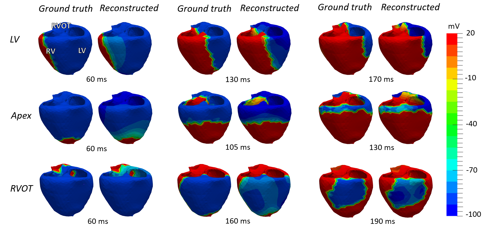
Figure 1. The ground truth transmembrane potential and the reconstructed transmembrane potentials recomputed by the extracellular potential under the isotropic assumptions. LV, the left ventricle; RV, the right ventricle; RVOT the right ventricle outflow tract.

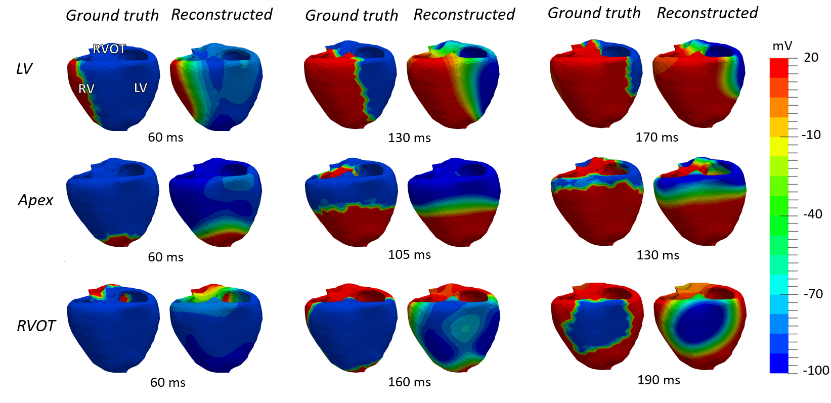
Figure 2. The ground truth transmembrane potential and the reconstructed transmembrane potentials recomputed by the electrical potential on the body surface under the isotropic assumptions. LV, the left ventricle; RV, the right ventricle; RVOT the right ventricle outflow tract.

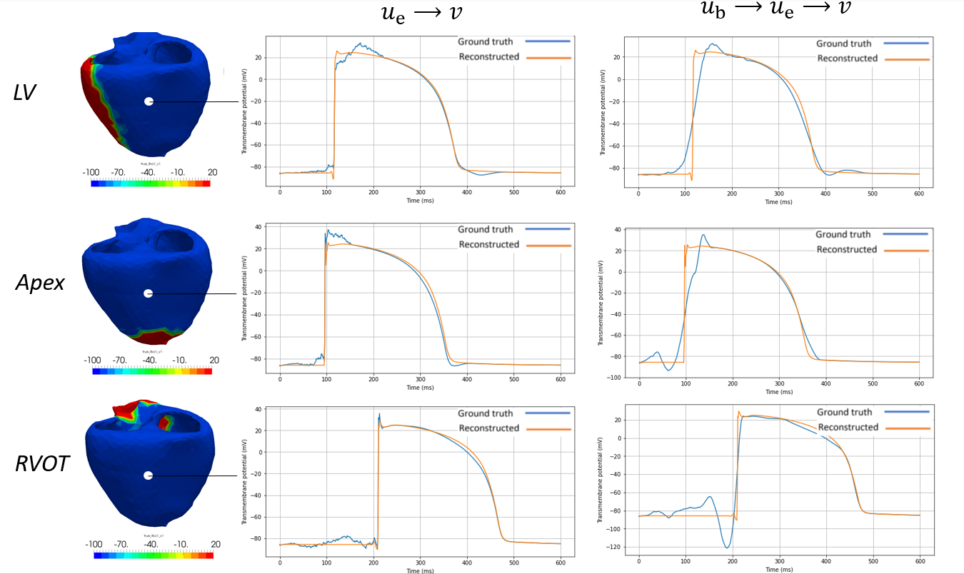
Figure 3. Examples of the ground truth and reconstructed transmembrane potential signals in a point in the center of the posterior-lower region of the ventricles of the heart.

This results shows the possibility of a sufficiently accurate reconstruction of the transmembrane potential based on the extracellular potential on the cardiac surface under the assumption of isotropic intracellular and extracellular electrical conductivity. The maximum reconstruction errors were observed in the vicinity of the spike of the transmembrane potential signal, while the up-stroke of the signal was reconstructed with high accuracy. Probably the precision of the reconstruction can be improved by using more optimal values for $m_{i}$ and $m_{e}$.

Results of the second evaluation protocol are presented in Tble 1 and shown in Figures 2 and 3. As expected, the accuracy of the reconstruction of the transmembrane potential was less than in the previous case. At the same time, the reconstructed transmebrane potential correctly conveys the sequence of the myocardial activation and the basic shape of the exact transmembrane potential signals.

The main component of the solution distorsion was the smoothness of the activation front and, accordingly, the upstroke of the transmembrane signals. Such pattern of the reconstructed solution is typical for the Tikhonov regularization. This fact suggests that the application of more advanced regularization algorithms. For investigation of the regularisation methods a theory of bases with double orthogonality in the Cauchy problem for elliptic operators (see [52]) can be useful.

5. Discussion and conclusion

Currently, methods for computational reconstruction of electrical activity of the heart inside the myocardium are being intensively developed based on the numerical solution of inverse problems for the bidomain model in various statements. This raises an important question about the theoretical limit of researchers’ endeavors in this direction. In particular, the established uniqueness theorems for the inverse problems are very important because it provides the basis for numerical computations. In contrast to the “forward” initial-boundary value problem for the bidomain equations the uniqueness of the solution of inverse problems has not been sufficiently studied. In this work, we aimed to eliminate this gap and provide some mathematical background for both the facts that are well adopted in the engineering community and some new ideas providing a substantial progress in computations.

The non-uniqueness of the solution of the inverse problem of reconstruction of the transmembrane potential inside the myocardium for the second-order elliptic equation of the bidomain model were shown in several previous works [42],[11],[25]. In this paper, we generalized these results by presenting a complete description of the null-space of the problem for the case of anisotropic electrical conductivity (Proposition 2.2). As a consequence, we also showed the uniqueness of the reconstruction of the action potential on the surface of the myocardium from the known electrical potential on the surface of the body.

Note that the electrical activity of the heart, even on its surface, provides valuable electrophysiological information about the patterns of cardiac excitation and the mechanisms of cardiac arrhythmias. In contrast to the electrical potential, the transmembrane potential more accurately characterizes the local electrical activity of the myocardium, especially the processes of myocardial repolarization. Therefore, the reconstruction of the transmembrane potential on the surface of the heart, the feasibility of which was justified in this article, can be useful for medical applications.

We illustrated the method for reconstruction of the transmembrane potential on the myocardial surface by the numerical experiments using the data of personalised modelling of electrical activity of the human heart ventricles. The reconstruction method were robust with respect to the model error associated with the ”isotropic” approximation of tensors of the extracellular and intracellular electrical conductivity.

From mathematical point of view, Proposition 2.2 states that the steady part of the bidomain model has too many degrees of freedom. This means that some of the necessary information about the desired solution is missing. Some approaches to complete this information were proposed in [42],[11], [2].

In this paper we considered two other possible ways to ensure the uniqueness of the solution of the problem. The first way consists of introducing the additional fourth order strongly elliptic equation. We gave an example to show a fact that the forth order elliptic equation can be obtained by applying the continuity equation in electromagnetism to the bidomain equations. The second way is to consider the original evolutionary form of the bidomain model.

The consideration were performed under very restrictive assumptions. Namely, we used the ”monodomain” assumption about of the proportionality of the electrical conductivity tensors and we utilized a linear version of the activation function of the bidomain model.

These simplifications are significant limitations of this study. However, some positive results on the uniqueness of the solution obtained for this highly simplified model show the prospects for further research in this direction.

Acknowledgments  The second author was supported by the Russian Science Foundation, grant N 20-11-20117.

References

- [1] Aliev, R.R., Panfilov, A.V., A simple two-variable model of Cardiac Excitation, Chaos, Solitons and Fractals, V. 7:3 (1996), 293–301.
- [2] Ainseba A., Bendahmane M., Lopez A. On 3D Numerical Inverse Problems for the Bidomain Model in Electrocardiology. Computers and Mathematics with Applications. 2015; 69 (4): 255–274.
- [3] Ainseba, B., Bendahmane, M., He, Y. Stability of conductivities in an inverse problem in the reaction-diffusion system in electrocardiology. Netw. Heterog. Media. 2015; 10: 369–385.
- [4] Bayer JD, Blake RC, Plank G, Trayanova NA. A novel rule-based algorithm for assigning myocardial fiber orientation to computational heart models. Annals of biomedical engineering. 2012;40(10):2243–2254.
- [5] Bendahmane M., Karlsen H.K. Analysis of a class of degenerate reaction–diffusion systems and the bidomain model of cardiac tissue. Netw. Heterog. Media. 2006; 1: 185–218.
- [6] Bendahmane M., Mroué F., Saad M., Talhouk R. Unfolding homogenization method applied to physiological and phenomenological bidomain models in electrocardiology. Nonlinear Analysis: Real World Applications.2019; 50: 413–447.
- [7] Beheshti M, Umapathy K, Krishnan S. Electrophysiological Cardiac Modeling: A Review. Crit Rev Biomed Eng. 2016; 44(1–2):99–122.
- [8] Borsuk, M. Transmission problem for Elliptic second-order Equations in non-smooth domains, Birkhäuser, Berlin, 2010.
- [9] Boulakia M, Cazeau S, Fernández MA, Gerbeau JF, Zemzemi N. Mathematical modeling of electrocardiograms: a numerical study., Annals of biomedical engineering. 2010;38(3):1071–1097.
- [10] Bourgault Y., Coudière Y., Pierre C. Existence and uniqueness of the solution for the bidomain model used in cardiac electrophysiology. Nonlinear Analysis: Real World Appl. 2009; 10(1), 458–482.
- [11] Burger, M., Mardal, K.A., Nielsen, B.F., Stability analysis of the inverse transmembrane potential problem in electrocardiography, Inverse Problems, 26(2010), 10, 105012
- [12] R.H. Clayton, O. Bernus, E.M. Cherry, at al. Models of cardiac tissue electrophysiology: Progress, challenges and open questions. Progress in Biophysics and Molecular Biology. 2011; 104(1–3):22–48.
- [13] Cluitmans M., Brooks D., MacLeod R., et al. Validation and Opportunities of Electrocardiographic Imaging: From Technical Achievements to Clinical Applications, Frontier in Physiology. 2018; 9: 1305.
- [14] Collin A., Imperiale S. Mathematical analysis and 2–scale convergence of an heterogeneous microscopic bidomain model. Math. Models Meth. Appl. Sci. 2018; (5)28:979–1035.
- [15] Colli-Franzone P., Savaré G. Degenerate evolution systems modeling the cardiac electric field at micro- and macroscopic level. In: Lorenzi A., Ruf B. (eds) Evolution Equations, Semigroups and Functional Analysis. Progress in Nonlinear Differential Equations and Their Applications, vol. 50. Birkhäuser, Basel, 2002.
- [16] Eidel’man, S.D., Parabolic equations, Partial differential equations – 6, Itogi Nauki i Tekhniki. Ser. Sovrem. Probl. Mat. Fund. Napr., 63, VINITI, Moscow, 1990, 201–313.
- [17] Fedchenko D.P., Shlapunov A.A., On the Cauchy problem for the elliptic complexes in spaces of distributions. Complex Variables and Elliptic Equations, V. 59, N. 5, 2014, 651-679.
- [18] Friedman, A., Partial differential equations of parabolic type, Englewood Cliffs, NJ, Prentice-Hall, Inc., 1964.
- [19] Geselowitz, D.B., Miller, V., A bidomain model for isotropic cardiac muscle, Ann. Biomed. Eng., 1983; 11 (3-4), 191-206.
- [20] Gilbarg, D., Trudinger, N., Elliptic Partial Differential Equations of second order, Berlin, Springer-Verlag, 1983.
- [21] Grandelius E., Karlsen K.H. The cardiac bidomain model and homogenization. Networks and Heterogeneous Media. 2019; 14(1): 173–204.
- [22] Hand P.E., Griffith B.E., Peskin C.S. Deriving macroscopic myocardial conductivities by homogenization of microscopic models. Bull Math Biol. 2009; 71(7):1707-26.
- [23] Hedberg, L.I., Wolff, T.H., Thin sets in nonlinear potential theory, Ann. Inst. Fourier (Grenoble) 33 (1983), no. 4, 161–187.
- [24] He, B., Li, G., and Zhang, X. Noninvasive imaging of cardiac transmembrane potentials within three-dimensional myocardium by means of a realistic geometry anisotropic heart model. IEEE Trans. Biomed. Eng. 2003; 50(10): 1190–1202.
- [25] Kalinin, V., Kalinin A., Schulze W.H.W., Potyagaylo D., Shlapunov, A., On the correctness of the transmembrane potential based inverse problem of ECG, Computing in Cardiology, 2017, 1–4.
- [26] Kalinin A., Potyagaylo D., Kalinin V., Solving the Inverse Problem of Electrocardiography on the Endocardium Using a Single Layer Source. Front Physiol. 2019; 10: 58.
- [27] Keller DU, Weiss DL, Dossel O, Seemann G. textit Influence of Heterogeneities on the Genesis of the T-wave: A Computational Evaluation. IEEE Transactions on Biomedical Engineering. 2012;59(2):311–322.
- [28] Kozlov, V.A., Maz’ya V.G., and Fomin, A.V., An iterative method for solving the Cauchy problem for elliptic equations, USSR Computational Mathematics and Mathematical Physics, 1991, 31:1, 45–52
- [29] Krassowska W., Neu J.C. Effective boundary conditions for syncytial tissues. IEEE Trans Biomed Eng. 1994; 41(2):143–50.
- [30] Kunisch K., Wagner M. Optimal control of the bidomain system (II): uniqueness and regularity theorems for weak solutions. Annali di Matematica Pura ed Applicata. 2013; 192: 951–986.
- [31] Kunisch K., Wagner M. Optimal control of the bidomain system. III: Existence of minimizers and first-order optimality conditions. ESAIM: Mathematical Modelling and Numerical Analysis. 2013; 47(4): 1077–1106.
- [32] Kurilenko, I.A., Shlapunov, A.A., On Carleman-type Formulas for Solutions to the Heat Equation, Journal of Siberian Federal University, Math. and Phys., 12:4 (2019), 421–433.
- [33] Ladyzhenskaya, O.A., Solonnikov V.A., Ural’tseva, N.N. Linear and Quasilinear Equations of Parabolic Type, Moscow, Nauka, 1967.
- [34] Lavrent’ev, M.M., On the Cauchy problem for linear elliptic equations of the second order, Dokl. AN SSSR, 112:2 (1957), 195–197.
- [35] Lions, J.-L., Quelques méthodes de résolution des problèmes aux limites non linéare, Dunod/Gauthier-Villars, Paris, 1969, 588 pp.
- [36] Lions, J. L., and Magenes, E., Non-Homogeneous Boundary Value Problems und Applications. Vol. 1, Springer-Verlag, Berlin et al., 1972.
- [37] Liu Z, Liu C, He B. Noninvasive reconstruction of three–dimensional ventricular activation sequence from the inverse solution of distributed equivalent current density. IEEE Trans Med Imaging. 2006; 25(10): 1307–18.
- [38] Maz’ya, V.G. and Havin, V.P. On the solutions of the Cauchy problem for Laplace’s equation (uniqueness, normality, approximation), Transactions of the Moscow Math. Soc., Vol 30 (1974), 65–118.
- [39] McLean, W., Strongly Elliptic Systems and Boundary Integral Equations, Cambridge Univ. Press, Cambridge, 2000.
- [40] Mikhailov, V.P., Partial differential equations, Nauka, Moscow, 1976.
- [41] Miller W.T, Geselowitz D.B. A bidomain model for anisotropic cardiac muscle. Ann Biomed. Eng. 1983; 11:191-–206.
- [42] Nielsen B.F., Cai X., Lysaker M. On the possibility for computing the transmembrane potential in the heart with a one-shot method: an inverse problem. Mathematical Biosciences. 2007; 210(2):523–553.
- [43] Neu J., Krassowska W. Homogenization of syncitial tissues. Crit. Rev. Biomed. Eng. 1993; 21(2): 137–199.
- [44] Pargaei, M., Rathish Kumar, B.V. On the existence–uniqueness and computation of solution of a class of cardiac electric activity models. Int J Adv Eng Sci Appl Math. 2019; 11: 198–216
- [45] Pennacchio M, Savaré G, Franzone PC. Multiscale modeling for the bioelectric activity of the heart. SIAM J. Math. Anal. 2005; (4)37:1333–1370.
- [46] Potse M. Scalable and Accurate ECG Simulation for Reaction-Diffusion Models of the Human Heart. Front Physiol. 2018; 9:370.
- [47] Puzyrev, R.E., Shlapunov, A.A. On a mixed problem for the parabolic Lamé type operator. J. Inv. Ill-posed Problems, V. 23:6 (2015), 555–570.
- [48] Quarteroni A., Lassila T., Rossi S., Ruiz-Baier R. Integrated heart–coupling multiscale and multiphysics models for the simulation of the cardiac function. Comput. Methods Appl. Mech. Eng. 2017; 314: 345–407.
- [49] Rjasanov S.,Steinbach O. The Fast Solution of Boundary Integral Equations. New-York: Springer-Verlag, 2007; 296 p.
- [50] Roitberg, Ya., Elliptic Boundary Value Problems in Spaces of Distributions, Kluwer Academic Publishers, Dordrecht, NL, 1996.
- [51] Roth BJ. Electrical conductivity values used with the bidomain model ofcardiac tissue. IEEE Transactions on Biomedical Engineering. 1997;44(4):326–328.
- [52] Shlapunov A.A., Tarkhanov, N.N., Bases with double orthogonality in the Cauchy problem for systems with injective symbols, Proceedings LMS, 3(1995), 1, 1–52.
- [53] Shefer, Yu.L., On a Transmission Problem Related to Models of Electrocardiology, Journal of Siberian federal university. Math. and Physics, 13(2020), 5, 596–607.
- [54] Schmidt, O. Biological information processing using the concept of interpenetrating domains,In: Leibovic K.N. (eds) Information Processing in The Nervous System. Springer, Berlin, Heidelberg, 1969.
- [55] Simanca, S., Mixed Elliptic Boundary Value Problems, Comm. in PDE, 12(1987), 123–200.
- [56] Smale, S., An infnite dimensional version of Sard’s theorem, Amer. J. Math. 87 (1965), no. 4, 861–866.
- [57] Sundnes, J.,Lines, G.T.,Cai, X., Nielsen, B.F., Mardal, K.A., Tveito, A., Computing the Electrical Activity in the Heart, Springer-Verlag, 2006.
- [58] Slobodetskii, L. N., Generalised spaces of S.L. Sobolev and their applications to boundary problems for partial differential equations, Science Notes of Leningr. Pedag. Institute 197 (1958), 54–112.
- [59] Sveshnikov, A.G., Bogolyubov, A.N., Kravtsov, V.V., Lectures on mathematical physics, M., Nauka, 2004.
- [60] Tarkhanov, N., Complexes of Differential Operators, Kluwer Academic Publishers, Dordrecht, NL, 1995.
- [61] Tarkhanov, N., The Analysis of solutions of Elliptic Equations, Kluwer Academic Publishers, Dordrecht, NL, 1997.
- [62] Tarkhanov, N., The Cauchy Problem for Solutions of Elliptic Equations, Akademie-Verlag, Berlin, 1995.
- [63] Ten Tusscher KH, Panfilov AV. Alternans and spiral breakup in a human ventricular tissue model. American Journal of Physiology-Heart and Circulatory Physiology. 2006;291(3):H1088–H1100.
- [64] Tikhonov, A.N., Arsenin, V.Ya., Methods of Solving Ill-posed Problems, Nauka, Moscow,1986.
- [65] Trayanova N.A. Whole–heart modeling: applications to cardiac electrophysiology and electromechanics. Circ Res. 2011; 108(1): 113–28.
- [66] Tung, L. A bi-domain model for describing ischemic myocardial D-C potentials. Ph.D. dissertation, Massachusetts Inst. Technol., Cambridge, MA, 1978.
- [67] Ushenin K., Kalinin V., Gitinova S., et al. Parameter variations in personalized electrophysiological models of human heart ventricles. PLOS ONE. 2021; 16(4):e0249062.
- [68] Veneroni M. Reaction-diffusion systems for the macroscopic bidomain model of the cardiac electric field. Nonlinear Analysis: Real World Appli. 2009; 10(2): 849–868.
- [69] Wang L., Zhang H., Wong K., Liu, H., Shi, P. Physiological–model–constrained noninvasive reconstruction of volumetric myocardial transmembrane potentials. IEEE Trans. Biomed. Eng. 2010; 57(2): 296–315.
- [70] Wu, B., Yan, L., Gao, Y. et al. Carleman estimate for a linearized bidomain model in electrocardiology and its applications. Nonlinear Differ. Equ. Appl. 25, 4 (2018).
- [71] Yu L., Zhou Z., He B. Temporal Sparse Promoting Three Dimensional Imaging of Cardiac Activation. IEEE Trans Med Imaging. 2015; 34(11):2309–2319.
- [72] Cooper F.R., Baker R.E., et al. Chaste: cancer, heart and soft tissue environment. Journal of Open Source Software; 5(47): 1848.