A new baseline for retinal vessel segmentation: Numerical identification and correction of methodological inconsistencies affecting 100+ papers
Abstract
In the last 15 years, the segmentation of vessels in retinal images has become an intensively researched problem in medical imaging, with hundreds of algorithms published. One of the de facto benchmarking data sets of vessel segmentation techniques is the DRIVE data set. Since DRIVE contains a predefined split of training and test images, the published performance results of the various segmentation techniques should provide a reliable ranking of the algorithms. Including more than 100 papers in the study, we performed a detailed numerical analysis of the coherence of the published performance scores. We found inconsistencies in the reported scores related to the use of the field of view (FoV), which has a significant impact on the performance scores. We attempted to eliminate the biases using numerical techniques to provide a more realistic picture of the state of the art. Based on the results, we have formulated several findings, most notably: despite the well-defined test set of DRIVE, most rankings in published papers are based on non-comparable figures; in contrast to the near-perfect accuracy scores reported in the literature, the highest accuracy score achieved to date is 0.9582 in the FoV region, which is 1% higher than that of human annotators. The methods we have developed for identifying and eliminating the evaluation biases can be easily applied to other domains where similar problems may arise.
keywords:
vessel segmentation, numerical analysis, accuracy, retina1 Introduction
Retinal images provide a noninvasive way to detect and monitor various conditions and diseases of the eye and body, such as diabetes-related retinopathies, macular degeneration, glaucoma and hypertension (Abramoff et al., 2010). Consequently, the computer-aided (semi-)automatic analysis and screening of retinal images has become a highly popular field of study in medical imaging, with thousands of papers and algorithms focusing on various anatomical parts and degenerations observable in retinal images (Abramoff et al., 2010; Trucco et al., 2019). The popularity of the field can be illustrated by the numerous challenges on the segmentation and grading of retinal images in recent years, organized by data science competition platforms (such as the Diabetic Retinopathy Challenge on Kaggle111https://www.kaggle.com/c/diabetic-retinopathy-detection), and as special tracks of corresponding conferences (like ”IDRiD: Diabetic Retinopathy – Segmentation and Grading Challenge” (Porwal et al., 2020)).
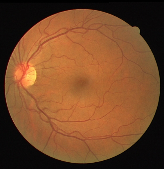
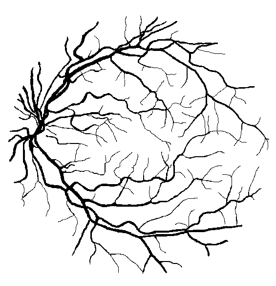
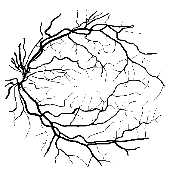

A particularly popular problem in retinal image analysis is the segmentation of retinal vessels (illustrated in Figure 1). The importance of the problem is threefold. On the one hand, the characteristics of the vasculature can aid the early detection of diseases like hypertension (lui Cheung et al., 2012). On the other hand, the removal of vessels usually precedes the detection of other anatomical parts. For example, the high curvature and junction points of thin vessels have similar visual features to microaneurysms (Long et al., 2020), consequently, the segmentation of the vasculature can indirectly aid the detection of mycroaneurysms. Finally, the segmented vasculature may serve as a guide for locating other anatomical parts, such as the macula (Yu et al., 2014).
In competitive research fields, where the primary goal is to find the most accurate solution to a problem, the proper comparison of algorithms is crucial. Comparability requires the coordination of evaluation data sets and methodologies that fit the purpose of the problem. As pointed out recently (Maier-Hein et al., 2018), even the grand challenges of recent years tend not to produce robust and reliable rankings. Therefore, the study of evaluations in active research areas such as retinal vessel segmentation is desirable to understand the state of the art.
In a self-organised fashion, three data sets have emerged as the de facto standard for the evaluation of vessel segmentation: DRIVE (Niemeijer et al., 2004), STARE (Hoover et al., 2000) and HRF (Budai et al., 2013). Of these, HRF is relatively new, and many classical algorithms have not yet been evaluated on it. STARE is not split into training and test sets, and the ambiguities of cross-validation lead to uncertain and hardly comparable results. In contrast, DRIVE eliminates many ambiguities of the evaluation by providing a predefined split of training and test images. Because of their long history, DRIVE and STARE continue to be the primary data sets for evaluation in recent work (Jin et al., 2019; Xiuqin et al., 2019), and due to predefined test set in DRIVE, the results obtained on DRIVE are generally accepted as comparable, which is reflected in the numerous rankings in the papers showing the merits of the newly proposed algorithms. The most commonly reported performance measures are the accuracy, sensitivity and specificity of the segmentation.
In a previous paper of ours (Kovács and Hajdu, 2016), we briefly pointed out that despite the predefined training and test sets in DRIVE, there is a potential methodological flaw in the evaluations, invalidating many rankings and comparisons in the literature. Namely, textual evidence suggests that some authors compute the performance scores in the field-of-view (FoV) region (Figure 1(d)), while others compute the scores for all pixels of the images (the entire rectangular area including the black surroundings of the FoV in Figure 1(d)). This minor difference affects the accuracy and specificity scores enormously. Due to the continued interest in this topic, we found it worthwhile to investigate the evaluation methodologies and their impact on comparability in detail. In this paper, we carry out a detailed numerical analysis of the phenomenon including more than 100 papers from the literature. In order to work with a sufficiently large population and eliminate the ambiguity of cross-validation, we investigate the accuracy, sensitivity and specificity scores reported for the test set of DRIVE. Our main contributions to the field can be summarized as follows:
-
1.
We introduce numerical approaches to uncover some details of the evaluation methodologies used in 100 relevant papers. The results provide inevitable evidence for two main types of methodologies with non-comparable performance scores: evaluation under the FoV mask and evaluation using all pixels.
-
2.
We attempt to eliminate the biases using numerical techniques to produce a more realistic ranking of algorithms.
-
3.
Our results confirm that most rankings in the literature are based on non-comparable figures, the state of the art performance cannot be deduced without the numerical inference and categorization of evaluation methodologies and adjustments of published figures.
-
4.
The techniques we introduce can be transferred to other areas where the identified methodological flaw is potentially present.
-
5.
According to our best knowledge, this is the first study investigating the coherence of a subfield of medical image analysis by numerical techniques.
-
6.
For complete reproducibility, the raw data, the implementation of the analysis and the results are shared in the GitHub repository https://github.com/gykovacs/retina_vessel_segmentation.
The paper is organized as follows. In Section 2, we describe the details of the data set DRIVE and formulate the problem we address by providing textual evidence for its existence. In Section 3, we introduce the numerical methods and present the raw results. Based on the findings of the numerical analysis, we discuss the state of the art in Section 4. Finally, we summarize the paper and draw conclusions in Section 5.
2 Problem formulation
In this section, we describe the main characteristics of the data set DRIVE, the performance scores, and we also discuss and illustrate the root cause of the problem we address.
2.1 The DRIVE data set
The Digital Retinal Images for Vessel Extraction (DRIVE) data set (Niemeijer et al., 2004) contains 20 training and 20 test entries. Images were captured with a Canon CR5 non-mydriatic 3CCD camera with a 45 degree field of view and cropped to 584565 pixels. Each training entry consists of a retinal image, a binary annotation of vessels (by annotator #1), and a binary mask of the Field of View (FoV) indicating the useful image content. The FoV masks cover 69% of the rectangular images. Each test entry includes an additional manual segmentation by annotator #2, enabling the evaluation of human annotators as a baseline. A complete entry from the test set is visualized in Figure 1.
2.2 Performance metrics
There are numerous metrics in the literature to characterize the performance of image segmentation algorithms. In retinal vessel segmentation, most authors report some metrics of binary classification performance at the pixel level. Particularly, a segmentation is compared to the ground truth image to determine the number of
-
•
true positives () - correctly identified vessel pixels;
-
•
true negatives () - correctly identified non-vessel pixels;
-
•
false positives () - non-vessel pixels identified as vessel;
-
•
false negatives () - vessel pixels identified as non-vessel;
and introducing and for the total number of vessel and non-vessel pixels, respectively, the scores
-
•
accuracy () - the proportion of all correctly identified pixels to all pixels;
-
•
sensitivity () - the proportion of correctly identified vessel pixels to all vessel pixels;
-
•
specificity () - the proportion of correctly identified non-vessel pixels to all non-vessel pixels
are reported at the image level or averaged on all test images. Some authors report the complements of the and scores known as false negative (1 - ) and false positive (1 - ) rates, respectively. We highlight that vessel segmentation as a binary classification problem is highly imbalanced, i.e., the number of vessel pixels in the FoV region is 15% of the number of non-vessel pixels, leading to high absolute accuracy and specificity scores: a 0.1% improvement in accuracy implies the correct segmentation of about 250 additional pixels, which is 1% of the size of the vasculature.
Since the goal is usually to maximize both sensitivity and specificity (and thus maximize accuracy), some authors report other composite measures of sensitivity and specificity, such as the F1-score (the harmonic mean of and ) or the AUC score (Hanley and Mcneil, 1982), however, these scores are reported too infrequently to rely a comprehensive analysis on them. Therefore, in the remainder of the paper, we focus on the , and scores.
2.3 The source of ambiguity
Although DRIVE specifies dedicated training and test sets, there is some ambiguity regarding the comparability of published performance scores. For example, one of the earliest papers (Staal et al., 2004) explicitly states: {quoting} ”Since the dark background outside the FOV is easily extracted, in this paper all experiments are done on the FOV only.” On the other hand, (Villalobos-Castaldi et al., 2010) says: {quoting} ”Based on a total of 329,960 pixels contained in a fundus image of size 565 584 pixels, it is possible to obtain the TP, TN, FP, and FN quantities of the segmented image.” Finally, the authors of (Yu et al., 2012) explicitly state that {quoting} ”It is mentionable that the accuracy and FPR [false positive rate] measures in Jiang (Jiang and Mojon, 2003), Martinez-Perez (Martinez-Perez et al., 2007), and Miri’s (Miri and Mahloojifar, 2010) methods were calculated in the complete image instead of the FOV.”
Even this handful of quotations suggests that some authors evaluate performance only in the area covered by the FoV mask, while others use all pixels of the images. The pixels outside the FoV are usually non-vessel pixels accounting for about 31% of all pixels in the images. If they are treated as true negatives, the accuracy and specificity increases tremendously. To illustrate the magnitude of this effect, we evaluate the segmentation of annotator #2 against annotation #1 (as ground truth) under the FoV mask and including all pixels of the images. With the FoV mask, , and , but using all pixels, , and . Omitting the FoV mask increased the and values by more than % and , respectively. The slight change in sensitivity is due to an average of 15 vessel pixels in the annotations #1 being outside the FoV. Since many authors report 0.1% improvements in accuracy, the variation in the region used for evaluation can cause an enormous bias when algorithms are compared and ranked.
In the rest of the paper, we develop numerical techniques to test the consistency of the published figures with the hypotheses that the authors either evaluated under the FoV mask or used all pixels of the images.
2.4 The need for the numerical analysis
We attempt to investigate the evaluation methodology of dozens of complex image processing pipelines. Collecting original implementations covering 15 years of technological development seems to be unmanagable. On the other hand, reimplementations of the algorithms are unlikely to reproduce the exact figures shared by the authors as all details of complex image processing pipelines are rarely shared due to length limitations. To avoid further bias and to treat all papers similarly and equally, we decided to base the study only on the shared performance scores. In order to draw conclusions without statistical uncertainties, we decided to rely on numerical analysis to reveal some details of the evaluation methodologies used by the authors.
3 Methods and raw results
In this section, the steps of the numerical analysis are described and the corresponding results are reported. The raw results are turned into insights and discussed in detail in Section 4. We introduce two special notations: The mean of a set of figures is denoted by an overline (such as standing for the mean of a set of accuracy scores), and asterisk indicates exact values with no uncertainty (such as standing for the exact number of true positives) that can either be extracted from the publicly available data set or denote unknown but exact values extracted by the authors to calculate the performance scores they reported.
3.1 The papers and algorithms involved
To select a sufficiently large, influential and comprehensive population of algorithms and reported performance scores without subjective bias, we applied the following strategy. We searched for the term retinal vessel segmentation in three of the largest scientific publication databases (Elsevier ScienceDirect, IEEE Xplore and ACM Digital Library) and recursively added the most cited ones with all algorithms referenced in them until we reached 90 papers. Finally, 10 recent papers, mainly based on deep learning have been added to represent the latest trends. To maintain quality and achieve the goals of our study, papers that met any of the following exclusion criteria were omitted in the selection process:
-
•
not sharing , and scores for DRIVE;
-
•
early papers of authors with multiple papers in the field;
-
•
being published only on preprint servers;
-
•
not reporting performance scores to at least 3 decimal places (rounding of the scores to 2 decimal places introduces larger uncertainty than the size of the bias we investigate).
|
Rank |
Key |
Num. image level |
Num. aggregated |
Annotator #2 acc. |
Region of eval. |
Decimal places |
Citations |
Rank |
Key |
Num. image level |
Num. aggregated |
Annotator #2 acc. |
Region of eval. |
Decimal places |
Citations |
||
| 1 | Jebaseeli et al. (2019) | .9898 | 1 | F | 4 | 6 | 51 | Meng et al. (2015) | .9529 | 20 | 1 | .9470 | F | 4 | 13 | ||
| 2 | Hassanien (2018) | .9793 | 20 | 1 | 4 | 24 | 52 | Li et al. (2016) | .9527 | 2 | 3 | .9472 | 4 | 306 | |||
| 3 | Wang et al. (2015) | .9767 | 20 | 9 | .9464 | F | 4 | 274 | 53 | Imani et al. (2015) | .9523 | 20 | 5 | .9473 | 4 | 84 | |
| 4 | Villalobos-Castaldi et al. (2010) | .9759 | 1 | .9473 | a | 4 | 70 | 54 | Singh and Srivastava (2016) | .9522 | 20 | 1 | a | 4 | 75 | ||
| 5 | Memari et al. (2017) | .9722 | 3 | .9464 | 4 | 23 | 55 | Mo and Zhang (2017) | .9521 | 2 | 3 | 4 | 68 | ||||
| 6 | Park et al. (2020) | .9706 | 1 | 4 | 2 | 56 | Isavand Rahmani et al. (2020) | .9521 | 1 | 4 | 0 | ||||||
| 7 | Jiang et al. (2019) | .9706 | 9 | .9637 | 4 | 9 | 57 | Dash et al. (2020) | .952 | 20 | 1 | 3 | 0 | ||||
| 8 | Atli and Gedik (2021) | .9689 | 2 | .9637 | 4 | 3 | 58 | Chalakkal and Abdulla (2017) | .9518 | 1 | 4 | 12 | |||||
| 9 | Moghimirad et al. (2011) | .9659 | 4 | 1 | .9473 | F | 4 | 44 | 59 | Singh and Srivastava (2017) | .9513 | 20 | 1 | a | 4 | 3 | |
| 10 | Xiuqin et al. (2019) | .9650 | 1 | 4 | 12 | 60 | Mapayi et al. (2015) | .9511 | 6 | .9473 | 4 | 50 | |||||
| 11 | Escorcia-Gutierrez et al. (2020) | .964 | 20 | 1 | 3 | 0 | 61 | Zhang and Chung (2018) | .9504 | 1 | .9472 | 4 | 53 | ||||
| 12 | Sreejini and Govindan (2015) | .9633 | 1 | .9470 | 4 | 47 | 62 | Bharkad (2017) | .9503 | 20 | 1 | 4 | 3 | ||||
| 13 | Saleh et al. (2011) | .9630 | 2 | .9473 | 4 | 68 | 63 | Barkana et al. (2017) | .9502 | 4 | 4 | .9470 | F | 4 | 72 | ||
| 14 | Kumar et al. (2016) | .9626 | 1 | 4 | 28 | 64 | Khan et al. (2016) | .9501 | 20 | 1 | .9473 | 4 | 18 | ||||
| 15 | Wankhede and Khanchandani (2015) | .9626 | 1 | .9473 | a | 4 | 19 | 65 | Song and Lee (2017) | .9499 | 1 | .9473 | 4 | 12 | |||
| 16 | Pandey et al. (2017) | .9623 | 1 | 4 | 24 | 66 | Kovács and Hajdu (2016) | .9494 | 5 | .9473 | F | 4 | 36 | ||||
| 17 | Narkthewan and Maneerat (2019) | .9617 | 20 | 1 | 4 | 2 | 67 | Roychowdhury et al. (2015) | .9494 | 1 | 4 | 153 | |||||
| 18 | Waheed et al. (2015) | .9616 | 20 | 1 | 4 | 23 | 68 | Brancati et al. (2018) | .949 | 5 | .947 | F | 3 | 0 | |||
| 19 | Xiang et al. (2014) | .9613 | 1 | .9612 | 4 | 7 | 69 | Nazari and Pourghassem (2013) | .9481 | 2 | .9470 | 4 | 12 | ||||
| 20 | Alom et al. (2019) | .9613 | 5 | 4 | 46 | 70 | Kaur and Mittal (2017) | .9480 | 1 | 4 | 12 | ||||||
| 21 | Tang et al. (2017) | .9611 | 20 | 1 | .9470 | 4 | 6 | 71 | Palanivel et al. (2020) | .9480 | 4 | .9470 | 4 | 1 | |||
| 22 | Samuel and Veeramalai (2019) | .9609 | 4 | .9470 | 4 | 14 | 72 | Fraz et al. (2012c) | .9480 | 2 | 3 | .9464 | F | 4 | 493 | ||
| 23 | Tamim et al. (2020) | .9607 | 20 | 1 | 4 | 1 | 73 | Shah et al. (2017) | .9479 | 1 | .9473 | 4 | 18 | ||||
| 24 | Zhu et al. (2017) | .9607 | 20 | 9 | 4 | 92 | 74 | Zhang et al. (2016) | .9476 | 2 | .9472 | F | 4 | 171 | |||
| 25 | Thangaraj et al. (2018) | .9606 | 20 | 1 | 4 | 16 | 75 | Shukla et al. (2020) | .9476 | 1 | .9473 | 4 | 3 | ||||
| 26 | Lupascu and Tegolo (2016) | .9606 | 40 | 2 | .9473 | 4 | 1 | 76 | Cheng et al. (2014) | .9474 | 6 | .9470 | 4 | 80 | |||
| 27 | Fan et al. (2017) | .960 | 2 | 3 | 7 | 77 | Zhou et al. (2017) | .9469 | 5 | .9473 | F | 4 | 33 | ||||
| 28 | Lupaşcu et al. (2010) | .9597 | 7 | 1 | .9473 | 4 | 329 | 78 | Melinscak et al. (2015) | .9466 | 1 | 4 | 118 | ||||
| 29 | Ricci and Perfetti (2007) | .9595 | 2 | 1 | .9473 | F | 4 | 769 | 79 | Mendonca and Campilho (2006) | .9463 | 2 | .9473 | F | 4 | 983 | |
| 30 | Wu et al. (2020) | .9582 | 3 | 4 | 9 | 80 | Rezaee et al. (2017) | .9463 | 1 | .9473 | 4 | 34 | |||||
| 31 | Fathi and Naghsh-Nilchi (2013) | .9581 | 20 | 1 | 4 | 95 | 81 | Rahebi and Hardalaç (2014) | .9461 | 20 | 1 | 4 | 38 | ||||
| 32 | Dash and Bhoi (2018) | .957 | 20 | 1 | 3 | 14 | 82 | Miri and Mahloojifar (2010) | .9458 | 1 | 4 | 291 | |||||
| 33 | Budai et al. (2013) | .957 | 1 | .947 | 3 | 207 | 83 | Strisciuglio et al. (2016) | .9454 | 5 | 4 | 64 | |||||
| 34 | Noh et al. (2019) | .9569 | 1 | .9472 | 4 | 18 | 84 | Marin et al. (2011) | .9452 | 20 | 1 | F | 4 | 906 | |||
| 35 | Soomro et al. (2019) | .956 | 1 | 3 | 17 | 85 | Adapa et al. (2020) | .9450 | 20 | 1 | 4 | 4 | |||||
| 36 | Frucci et al. (2017) | .956 | 1 | 3 | 3 | 86 | Javidi et al. (2017) | .9450 | 1 | .9473 | F | 4 | 46 | ||||
| 37 | Frucci et al. (2016) | .955 | 20 | 1 | 3 | 27 | 87 | Azzopardi et al. (2015) | .9442 | 3 | 4 | 445 | |||||
| 38 | Saroj et al. (2020) | .9544 | 20 | 1 | 4 | 1 | 88 | Strisciuglio et al. (2015) | .9442 | 1 | 4 | 25 | |||||
| 39 | Yan et al. (2018) | .9542 | 2 | .9472 | 4 | 92 | 89 | Staal et al. (2004) | .9441 | 1 | .9473 | F | 4 | 2830 | |||
| 40 | Zhao et al. (2015b) | .954 | 5 | .947 | 3 | 246 | 90 | You et al. (2011) | .9434 | 1 | .9473 | F | 4 | 325 | |||
| 41 | Na et al. (2018) | .954 | 1 | .947 | 3 | 6 | 91 | Soomro et al. (2017) | .9432 | 1 | 4 | 21 | |||||
| 42 | Panda et al. (2016) | .9539 | 4 | .9470 | a | 4 | 32 | 92 | Kumar et al. (2020) | .9432 | 20 | 1 | .9473 | F | 4 | 0 | |
| 43 | GeethaRamani and Bal/an (2016) | .9536 | 20 | 1 | .9470 | 4 | 77 | 93 | Fraz et al. (2012a) | .9430 | 2 | 11 | .9473 | F | 4 | 294 | |
| 44 | Liskowski and Krawiec (2016) | .9535 | 12 | .9473 | F | 4 | 492 | 94 | Dai et al. (2015) | .9418 | 1 | 4 | 41 | ||||
| 45 | Soomro et al. (2018) | .9534 | 4 | 4 | 45 | 95 | Anzalone et al. (2008) | .9418 | 1 | .9473 | F | 4 | 57 | ||||
| 46 | Dasgupta and Singh (2017) | .9533 | 1 | 4 | 133 | 96 | Dizdaroglu et al. (2012) | .9412 | 2 | 4 | 25 | ||||||
| 47 | Ngo and Han (2017) | .9533 | 1 | 4 | 19 | 97 | Salazar et al. (2014) | .9412 | 1 | .9473 | F | 4 | 222 | ||||
| 48 | Hu et al. (2018) | .9533 | 4 | .9470 | F | 4 | 87 | 98 | Emary et al. (2014) | .939 | 20 | 1 | 3 | 26 | |||
| 49 | Yang et al. (2020) | .9532 | 4 | 4 | 0 | 99 | Zhang et al. (2010) | .9382 | 1 | .9473 | F | 4 | 530 | ||||
| 50 | Zhao et al. (2015a) | .953 | 10 | .947 | 3 | 91 | 100 | Odstrcilik et al. (2013) | .9340 | 20 | 1 | .9473 | a | 4 | 266 |
A summary of the papers in Table 1 shows some interesting insights into the evaluation methodologies. Authors rarely phrase explicitly the region they use for evaluation, and when it is shared, a mixture of the two edge cases can be observed: the use of the FoV, and evaluation on all pixels. When the region of evaluation is not shared, one can still observe the two accuracy scores 0.9473 and 0.9637 for annotator #2 (the scores we calculated in subsection 2.3 under the FoV and using all pixels, repsectively). Finally, a slight variation can be observed in the scores being close to the one computed under the FoV (0.9473). This suggests that custom adjustments to the FoV may also have occured, but there is no textual evidence or indication of the nature of these adjustments.
3.2 Overview of the numerical analysis
The analysis is based on the interdependence of the scores , and . Particularly, these scores cannot take arbitrary values: they are linear functions of the four unknowns , , and , which need to sum up to the number of positive (vessel) and negative (non-vessel) pixels, while needs to match the size of the FoV mask or the size of the image. Consequently, the reported values of a triplet of , and together with the exact number of positive and negative pixels in the images must satisfy certain conditions. In the rest of the section, this idea is developed further to deal with the numerical uncertainties of rounding and averaging, and to allow inferences to be made about the evaluation methodologies.
3.3 Image level analysis
Some authors have reported the , and scores at the image level. In this subsection, we develop a consistency test to decide whether the image level scores were computed in the FoV region or using all pixels of the images.
3.3.1 The image level consistency test
For each image, the true positives () and true negatives () calculated by the authors must satisfy the following inequalities by definition:
| (1) | ||||
| (2) | ||||
| (3) | ||||
| (4) |
where the total number of positive (vessel) and negative (non-vessel) pixels can be determined given the publicly available images, and denotes the numerical uncertainty of the reported figures. The setting is the maximum numerical uncertainty when the figures reported to decimal places are subject to rounding, and is the maximum uncertainty when truncation or ceiling to decimal places is assumed.
Eliminating and from the inequalities gives 6 conditions that must hold for a given triplet of , and scores, regardless of the actual values of and :
| (5) |
The conditions (5) allow us to test the consistency of a certain triplet of , and reported for an image with positives and negatives, with numerical uncertainty. Since we are concerned about two cases (evaluation using the FoV mask or all pixels), one can extract the total number of positives and negatives with and without the FoV and test whether the conditions for either hypothesis are satisfied. For example, treating annotation #1 as ground truth and annotation #2 as a segmentation for the test image in Figure 1, the rounded performance scores with the FoV mask are , , . In the FoV region, and , and substituting these figures into the inequalities (5), all conditions are satisfied. On the other hand, including all pixels of the images, and , and with this substitution the conditions fail.
The conditions (5) are sharp in the sense that if the assumptions on and are correct, then the conditions must hold; if the assumptions on and are sufficiently far the figures used to compute the scores , and , then the test fails. However, due to the numerical uncertainty, scores computed in regions slightly different from the assumptions might also satisfy the conditions (5). This phenomenon is examined in the next subsection.
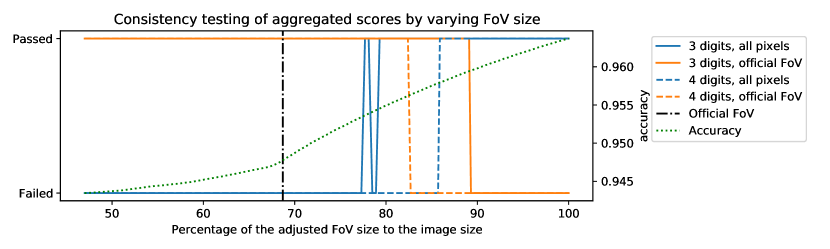
3.3.2 Sensitivity of the image level consistency test
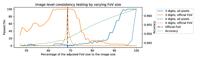
To quantitatively characterize the sensitivity of the test to changes in the region of evaluation, we carried out a simulation treating annotation #1 as ground truth and annotation #2 as segmentation for all 20 images in the DRIVE test set. The FoV masks were gradually dilated to cover the images; for each mask size, the performance scores were calculated and rounded to 3 and 4 digits; and the tests derived in subsection 3.3.1 were applied to the scores to check whether they were computed under the original FoV masks or using all pixels of the images. The percentages of image level scores passing the tests at certain mask sizes are plotted in Figure 2 along with the average accuracy to illustrate the bias caused by the adjustment of evaluation region. The first thing to observe is that varying the size of the evaluation region has a remarkable effect on the accuracy scores. However, when the performance scores are rounded to 4 digits, a deviation as little as 1% from the assumed region makes the test fail on more than 50% of the 20 test images, as can be seen by the steep drop in the corresponding dashed lines around the size of the official FoVs (69% of the image size) and at 100% of the image size. The increased uncertainty of rounding to 3 digits widens the acceptance window (solid lines) and about 50% of the scores pass despite a 15% change in the size of the evaluation region. However, the passing rate drops to about 5% at the opposite assumptions, indicating that the two edge cases can still be distinguished by the test. The analysis suggests that the consistency test is able to distinguish the cases where the official (or slightly differing) FoV masks were used from those cases when all (or almost all) pixels of the images were included in the evaluation.
| Key |
Decimal places |
Num. image level fig. |
% passed assum. FoV |
% passed assum. all pixels |
Decision | |||
|---|---|---|---|---|---|---|---|---|
| Hassanien (2018) | .9793 | .8981 | .9883 | 4 | 20 | 0 | 5 | outlier |
| Wang et al. (2015) | .9767 | .8173 | .9733 | 4 | 20 | 0 | 0 | outlier |
| Moghimirad et al. (2011) | .9659 | .7852 | .9935 | 4 | 4 | 25 | 25 | outlier |
| Escorcia-Gutierrez et al. (2020) | .9640 | .6170 | .9980 | 3 | 20 | 0 | 0 | outlier |
| Narkthewan and Maneerat (2019) | .9617 | .6392 | .9920 | 4 | 20 | 0 | 5 | outlier |
| Waheed et al. (2015) | .9616 | .7937 | .9779 | 4 | 20 | 0 | 90 | all pixels |
| Tang et al. (2017) | .9611 | .8174 | .9747 | 4 | 20 | 0 | 10 | outlier |
| Tamim et al. (2020) | .9607 | .7542 | .9843 | 4 | 20 | 0 | 0 | outlier |
| Zhu et al. (2017) | .9607 | .7140 | .9868 | 4 | 20 | 0 | 0 | outlier |
| Thangaraj et al. (2018) | .9606 | .8014 | .9753 | 4 | 20 | 0 | 10 | outlier |
| Lupascu and Tegolo (2016) | .9606 | .7006 | .9857 | 4 | 40 | 0 | 82 | all pixels |
| Lupaşcu et al. (2010) | .9597 | .6728 | .9874 | 4 | 7 | 0 | 57 | all pixels |
| Ricci and Perfetti (2007) | .9595 | .7283 | .9832 | 4 | 2 | 0 | 50 | outlier |
| Fathi and Naghsh-Nilchi (2013) | .9581 | .7768 | .9759 | 4 | 20 | 0 | 100 | all pixels |
| Dash and Bhoi (2018) | .9570 | .7410 | .9860 | 3 | 20 | 15 | 10 | outlier |
| Frucci et al. (2016) | .9550 | .6400 | .9850 | 3 | 20 | 0 | 100 | all pixels |
| Saroj et al. (2020) | .9544 | .7307 | .9761 | 4 | 20 | 0 | 100 | all pixels |
| GeethaRamani and Bal/an (2016) | .9536 | .7079 | .9778 | 4 | 20 | 0 | 85 | all pixels |
| Meng et al. (2015) | .9529 | .7489 | .9818 | 4 | 20 | 5 | 0 | outlier |
| Li et al. (2016) | .9527 | .7569 | .9816 | 4 | 2 | 100 | 0 | FoV |
| Imani et al. (2015) | .9523 | .7524 | .9753 | 4 | 20 | 0 | 0 | outlier |
| Singh and Srivastava (2016) | .9522 | .7594 | .9708 | 4 | 20 | 0 | 100 | all pixels |
| Mo and Zhang (2017) | .9521 | .7760 | .9779 | 4 | 2 | 100 | 0 | FoV |
| Dash et al. (2020) | .9520 | .7560 | .9810 | 3 | 20 | 25 | 15 | outlier |
| Singh and Srivastava (2017) | .9513 | .7171 | .9739 | 4 | 20 | 0 | 100 | all pixels |
| Bharkad (2017) | .9503 | .7278 | .9718 | 4 | 20 | 0 | 100 | all pixels |
| Barkana et al. (2017) | .9502 | .7224 | .9840 | 4 | 4 | 0 | 0 | outlier |
| Khan et al. (2016) | .9501 | .7373 | .9670 | 4 | 20 | 0 | 5 | outlier |
| Fraz et al. (2012c) | .9480 | .7406 | .9807 | 4 | 2 | 0 | 0 | outlier |
| Rahebi and Hardalaç (2014) | .9461 | .7365 | .9707 | 4 | 20 | 5 | 0 | outlier |
| Marin et al. (2011) | .9452 | .7067 | .9801 | 4 | 20 | 100 | 0 | FoV |
| Adapa et al. (2020) | .9450 | .6994 | .9811 | 4 | 20 | 100 | 0 | FoV |
| Kumar et al. (2020) | .9432 | .7503 | .9717 | 4 | 20 | 100 | 0 | FoV |
| Fraz et al. (2012a) | .9430 | .7152 | .9769 | 4 | 2 | 50 | 0 | outlier |
| Emary et al. (2014) | .9390 | .7210 | .9710 | 3 | 20 | 100 | 0 | FoV |
| Odstrcilik et al. (2013) | .9340 | .7060 | .9693 | 4 | 20 | 0 | 0 | outlier |
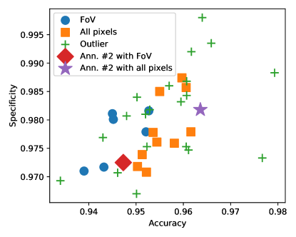
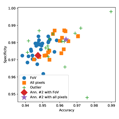
3.3.3 Image level results
The image level consistency test was applied to all image level figures shared by 36 authors. To tolerate possible typos in the published figures and minor deviations from the exact assumptions, the image level results are aggregated according to the following permissive rule. If the use of the FoV (all pixels) is confirmed by the majority of the image level scores shared in a paper, the published scores are accepted to be calculated under the FoV (all pixels). If none of the assumptions are confirmed by the majority of the image level scores passing, all results of the paper are marked as outliers in terms of evaluation: in these cases we can state with certainty that the authors evaluated in an unknown way.
The results are summarized in Table 2 and plotted in Figure 3 in the accuracy-specificity plane. Surprisingly, 20 out of the 36 papers with image level scores turned out to be outliers. The ranking in Table 2 shows that almost all papers where the use of all pixels was accepted outperform those evaluating under the FoV mask, clearly showing the expected skew in the evaluations. A similar pattern can be seen in Figure 3: the scores where the use of the FoV mask was accepted tend to have lower accuracy and specificity scores than those where the use of all pixels was confirmed.
3.4 The analysis of aggregated figures
Most authors report only the averages of image level performance scores. In this subsection, we develop consistency tests to take into consideration the numerical uncertainty caused by the averaging.
3.4.1 The consistency test for aggregated figures
The concept of the consistency test for the average scores is similar to that of the image level test. Given the exact number of positive (vessel) and negative (non-vessel) pixels for each image in the DRIVE test set, one can formulate conditions that must be satisfied if the evaluation was performed according to the assumptions about the region of evaluation. Let denote the number of positive and negative pixels in the manual annotation of the th image under a particular assumption (the use of the FoV or all pixels). If the assumption is true, the following conditions must be satisfiable for some , , unknown integers:
| (6) | |||
| (7) | |||
| (8) | |||
| (9) |
All these conditions are linear functions of the unknowns, thus, (6)-(9) can be interpreted as the condition set of a linear integer programming problem. In order to check if these conditions can be fulfilled, one can exploit any linear integer programming solver with a dummy objective function, and an empty feasibility set returned by the solver indicates that the conditions cannot be satisfied, thus, the aggregated performance scores are not consistent with the test images of DRIVE under the hypothesis (using the FoV or all pixels) which led to the and numbers.
| Key |
Decimal places |
Num. agg. figures |
Passed assum. FoV |
Passed assum. all pixels |
Decision | |||
|---|---|---|---|---|---|---|---|---|
| Jebaseeli et al. (2019) | .9898 | .8027 | .9980 | 4 | 1 | outlier | ||
| Villalobos-Castaldi et al. (2010) | .9759 | .9649 | .9480 | 4 | 1 | outlier | ||
| Memari et al. (2017) | .9722 | .8726 | .9884 | 4 | 1 | outlier | ||
| Park et al. (2020) | .9706 | .8346 | .9836 | 4 | 1 | + | all pixels | |
| Jiang et al. (2019) | .9706 | .8325 | .9838 | 4 | 1 | + | all pixels | |
| Atli and Gedik (2021) | .9689 | .7987 | .9854 | 4 | 1 | outlier | ||
| Xiuqin et al. (2019) | .9650 | .8150 | .9808 | 4 | 1 | + | all pixels | |
| Sreejini and Govindan (2015) | .9633 | .7132 | .9866 | 4 | 1 | + | all pixels | |
| Saleh et al. (2011) | .9630 | .8423 | .9658 | 4 | 1 | outlier | ||
| Kumar et al. (2016) | .9626 | .7006 | .9871 | 4 | 1 | + | all pixels | |
| Wankhede and Khanchandani (2015) | .9626 | .7261 | .9806 | 4 | 1 | outlier | ||
| Pandey et al. (2017) | .9623 | .8106 | .9761 | 4 | 1 | + | all pixels | |
| Alom et al. (2019) | .9613 | .7661 | .9807 | 4 | 1 | outlier | ||
| Xiang et al. (2014) | .9613 | .7538 | .9828 | 4 | 1 | + | all pixels | |
| Samuel and Veeramalai (2019) | .9609 | .8282 | .9738 | 4 | 1 | + | all pixels | |
| Fan et al. (2017) | .9600 | .7360 | .9810 | 3 | 1 | + | all pixels | |
| Wu et al. (2020) | .9582 | .7996 | .9813 | 4 | 1 | + | FoV | |
| Budai et al. (2013) | .9570 | .6440 | .9870 | 3 | 1 | + | all pixels | |
| Noh et al. (2019) | .9569 | .8354 | .9746 | 4 | 1 | + | FoV | |
| Soomro et al. (2019) | .9560 | .8700 | .9850 | 3 | 1 | outlier | ||
| Frucci et al. (2017) | .9560 | .6600 | .9850 | 3 | 1 | + | all pixels | |
| Yan et al. (2018) | .9542 | .7653 | .9818 | 4 | 1 | + | FoV | |
| Na et al. (2018) | .9540 | .7680 | .9700 | 3 | 1 | + | all pixels | |
| Zhao et al. (2015b) | .9540 | .7420 | .9820 | 3 | 1 | outlier | ||
| Panda et al. (2016) | .9539 | .7328 | .9752 | 4 | 1 | + | all pixels | |
| Liskowski and Krawiec (2016) | .9535 | .7811 | .9807 | 4 | 1 | + | FoV | |
| Soomro et al. (2018) | .9534 | .7592 | .9763 | 4 | 1 | outlier | ||
| Dasgupta and Singh (2017) | .9533 | .7691 | .9801 | 4 | 1 | + | FoV | |
| Hu et al. (2018) | .9533 | .7796 | .9717 | 4 | 1 | outlier | ||
| Ngo and Han (2017) | .9533 | .7464 | .9836 | 4 | 1 | + | FoV | |
| Yang et al. (2020) | .9532 | .7349 | .9743 | 4 | 1 | + | all pixels | |
| Zhao et al. (2015a) | .9530 | .7440 | .9780 | 3 | 1 | outlier | ||
| Isavand Rahmani et al. (2020) | .9521 | .7400 | .9726 | 4 | 1 | + | all pixels | |
| Chalakkal and Abdulla (2017) | .9518 | .7386 | .9769 | 4 | 1 | outlier | ||
| Mapayi et al. (2015) | .9511 | .7313 | .9724 | 4 | 1 | + | all pixels | |
| Zhang and Chung (2018) | .9504 | .8723 | .9618 | 4 | 1 | + | FoV | |
| Song and Lee (2017) | .9499 | .7501 | .9795 | 4 | 1 | + | FoV | |
| Roychowdhury et al. (2015) | .9494 | .7395 | .9782 | 4 | 1 | + | FoV | |
| Kovács and Hajdu (2016) | .9494 | .7450 | .9793 | 4 | 1 | + | FoV | |
| Brancati et al. (2018) | .9490 | .7820 | .9760 | 3 | 1 | + | FoV | |
| Nazari and Pourghassem (2013) | .9481 | .7112 | .9716 | 4 | 1 | + | all pixels | |
| Kaur and Mittal (2017) | .9480 | .8730 | .9869 | 4 | 1 | outlier | ||
| Palanivel et al. (2020) | .9480 | .7375 | .9788 | 4 | 1 | + | FoV | |
| Shah et al. (2017) | .9479 | .7205 | .9814 | 4 | 1 | + | FoV | |
| Zhang et al. (2016) | .9476 | .7743 | .9725 | 4 | 1 | + | FoV | |
| Shukla et al. (2020) | .9476 | .7015 | .9836 | 4 | 1 | + | FoV | |
| Cheng et al. (2014) | .9474 | .7252 | .9798 | 4 | 1 | + | FoV | |
| Zhou et al. (2017) | .9469 | .8078 | .9674 | 4 | 1 | + | FoV | |
| Melinscak et al. (2015) | .9466 | .7276 | .9785 | 4 | 1 | + | FoV | |
| Rezaee et al. (2017) | .9463 | .7189 | .9793 | 4 | 1 | + | FoV | |
| Mendonca and Campilho (2006) | .9463 | .7315 | .9781 | 4 | 1 | + | FoV | |
| Miri and Mahloojifar (2010) | .9458 | .7352 | .9795 | 4 | 1 | + | FoV | |
| Strisciuglio et al. (2016) | .9454 | .7777 | .9702 | 4 | 1 | + | FoV | |
| Javidi et al. (2017) | .9450 | .7201 | .9702 | 4 | 1 | + | all pixels | |
| Strisciuglio et al. (2015) | .9442 | .7655 | .9704 | 4 | 1 | + | FoV | |
| Azzopardi et al. (2015) | .9442 | .7655 | .9704 | 4 | 1 | + | FoV | |
| Staal et al. (2004) | .9441 | .7750 | .9725 | 4 | 1 | + | FoV | |
| You et al. (2011) | .9434 | .7410 | .9751 | 4 | 1 | + | FoV | |
| Soomro et al. (2017) | .9432 | .7523 | .9760 | 4 | 1 | + | FoV | |
| Dai et al. (2015) | .9418 | .7359 | .9720 | 4 | 1 | + | FoV | |
| Anzalone et al. (2008) | .9418 | .7286 | .9810 | 4 | 1 | outlier | ||
| Dizdaroglu et al. (2012) | .9412 | .7181 | .9743 | 4 | 1 | outlier | ||
| Salazar et al. (2014) | .9412 | .7512 | .9684 | 4 | 1 | + | FoV | |
| Zhang et al. (2010) | .9382 | .7120 | .9724 | 4 | 1 | + | FoV |
3.4.2 Sensitivity of the consistency test for aggregated figures
Similarly to the image level analysis, the aggregated figures must pass the test if the assumptions are met. However, due to the increased numerical uncertainty, it is questionable whether the sensitivity of the test is high enough to distinguish the two corner cases we are concerned with. As before, a quantitative characterization of sensitivity can be obtained by varying the size of the evaluation region, but this time checking whether the aggregated figures pass the test with the , , numbers extracted according to the hypotheses. According to the results shown in Figure 4, a 15% deviation in size from the hypothesised region causes the test to fail when the scores are reported to 4 digits. With rounding to 3 digits, the two corner cases are still distinguished by the test. However, if the region of evaluation is between 77%-87% of the image size, the scores can pass the test with either assumption.
3.4.3 The results on aggregated figures
In some papers (such as (Wu et al., 2020)), multiple triplets of aggregated scores are reported to illustrate the effects of the various steps of the proposed methods. Similarly to the image level analysis, the majority rule is applied to make clear decisions about the region of evaluation used by the authors. The results are summarized in Table 3 and plotted in Figure 5. Again, we assigned 3 labels to the papers, in 30 cases the use of the FoV was accepted, in 18 cases the use of all pixels was accepted, and 16 papers were classified as outliers (the scores do not pass the test with either of the hypothesised regions). As before, the ranking in Table 3 and the illustration in Figure 5 confirm the expected bias in the evaluations: the algorithms evaluated on all pixels tend to have higher accuracy and specificity scores, in general.
To assess the sensitivity of the aggregated consistency test compared to the image level test, we compared the categorization based on image level and aggregated figures and found that the aggregated consistency test gave the same result in all cases where the use of the FoV mask or all pixels was confirmed at the image level. However, from the total of 20 outliers identified at the image level, in 15 cases the aggregated scores passed the consistency test with one of the assumptions. This suggests that there can be further outliers among the papers in which only aggregated scores are reported and the consistency test confirmed one of the hypotheses.
3.5 An improved ranking
In this section, we attempt to derive a more realistic ranking of the algorithms by eliminating the bias caused by the differing regions of evaluation. The goal of the method we develop is to map the scores calculated on all pixels into the domain of evaluation with the FoV mask.
The idea is analogous to that of the consistency tests. Let the subscripts and refer to figures computed under the FoV mask and using all pixels, respectively, and let denote the difference. Given a particular triplet of image level scores , and reported by the authors with numerical uncertainty, we would like to infer on , and . Substituting the unknowns and into (1)-(4), one gets the conditions
| (10) |
which must hold for some integer unknowns and . The constants and are known from the publicly available test set. Focusing on the accuracy score first, we are interested in a lower and upper bound on the values it can take under the conditions (10). Recognizing that the conditions (10) with the objective function form a linear integer programming problem of the free integer variables and , one can determine the minimum () and maximum () values the objective function can take by exploiting any linear programming solver. These extrema provide a sharp interval estimate for the accuracy score evaluated under the FoV: . The adjusted accuracy score is defined as the mid-point of the interval and the error of the adjustment is estimated as the half-width of the interval:
| (11) |
The adjusted image level and scores and corresponding error estimates are determined analogously.
In practice, we found that the formulation (10) leads to wide intervals due to mathematical solutions that are not aligned with the problem. In the formulation (10), the number of true negatives outside the FoV () can be zero, that is, the linear programming solver considers variable configurations corresponding to segmentations where all pixels outside the FoV are segmented as vessels, which is unlikely. In order to tighten the intervals, the configuration space is reduced by making the natural assumption that no more negative pixels than 1% of the vasculature are segmented as vessels outside the FoV: . With this constraint, the worst-case error of the adjustment when applied to all image level figures reduces to with the average of 0.001, which we found sufficiently tight for further analysis.
Similarly to the image level adjustment, for the averaged scores, one can substitute and , into the conditions (6) - (9) leading to a set of linear integer constraints. Then, minimizing and maximizing the objective function
| (12) |
in the free integer variables , , one gets a sharp interval estimate for . The adjusted aggregated score is determined as the mid-point of the interval and the corresponding error term as the half-width of the interval. The adjusted and scores are determined analogously.
For illustration, the adjustment was applied to the scores calculated on all pixels and reported in our earlier paper (Kovács and Hajdu, 2016). The adjusted scores , , are well aligned with the true scores , , calculated in the FoV area, the error of the adjustment is not higher than for any of the figures.
The adjustment was applied to the reported scores of all methods we identified to be evaluated using all pixels. The worst case of the adjustment is with the average of . As the errors are an order of magnitude smaller than the bias, we believe that the ranking based on the adjusted scores in Table 4 is a more reliable baseline for the field than the original ranking in Table 1.
| Key |
Rank |
Original rank |
Rank diff. |
Adjusted acc. |
Published acc. |
Category | Operation |
|---|---|---|---|---|---|---|---|
| Wu et al. (2020) | 1 | 30 | 29 | .9582 | .9582 | FoV | deep learning |
| Park et al. (2020) | 2 | 6 | 4 | .9578 | .9706 | all pixels | deep learning |
| Jiang et al. (2019) | 3 | 7 | 4 | .9578 | .9706 | all pixels | deep learning |
| Noh et al. (2019) | 4 | 34 | 30 | .9569 | .9569 | FoV | deep learning |
| Yan et al. (2018) | 5 | 39 | 34 | .9542 | .9542 | FoV | deep learning |
| Liskowski and Krawiec (2016) | 6 | 44 | 38 | .9535 | .9535 | FoV | deep learning |
| Ngo and Han (2017) | 7 | 47 | 40 | .9533 | .9533 | FoV | deep learning |
| Dasgupta and Singh (2017) | 8 | 46 | 38 | .9533 | .9533 | FoV | deep learning |
| Li et al. (2016) | 9 | 52 | 43 | .9527 | .9527 | FoV | deep learning |
| Mo and Zhang (2017) | 10 | 55 | 45 | .9521 | .9521 | FoV | deep learning |
| Xiuqin et al. (2019) | 11 | 10 | -1 | .9505 | .9650 | all pixels | deep learning |
| Zhang and Chung (2018) | 12 | 61 | 49 | .9504 | .9504 | FoV | deep learning |
| Song and Lee (2017) | 13 | 65 | 52 | .9499 | .9499 | FoV | deep learning |
| Roychowdhury et al. (2015) | 14 | 67 | 53 | .9494 | .9494 | FoV | classical |
| Kovács and Hajdu (2016) | 15 | 66 | 51 | .9494 | .9494 | FoV | classical |
| Brancati et al. (2018) | 16 | 68 | 52 | .9490 | .9490 | FoV | deep learning |
| Palanivel et al. (2020) | 17 | 71 | 54 | .9480 | .9480 | FoV | supervised |
| Shah et al. (2017) | 18 | 73 | 55 | .9479 | .9479 | FoV | supervised |
| Zhang et al. (2016) | 19 | 74 | 55 | .9476 | .9476 | FoV | classical |
| Shukla et al. (2020) | 20 | 75 | 55 | .9476 | .9476 | FoV | classical |
| Cheng et al. (2014) | 21 | 76 | 55 | .9474 | .9474 | FoV | supervised |
| Sreejini and Govindan (2015) | 22 | 12 | -10 | .9471 | .9633 | all pixels | classical |
| Zhou et al. (2017) | 23 | 77 | 54 | .9469 | .9469 | FoV | other |
| Melinscak et al. (2015) | 24 | 78 | 54 | .9466 | .9466 | FoV | deep learning |
| Rezaee et al. (2017) | 25 | 80 | 55 | .9463 | .9463 | FoV | classical |
| Mendonca and Campilho (2006) | 26 | 79 | 53 | .9463 | .9463 | FoV | classical |
| Kumar et al. (2016) | 27 | 14 | -13 | .9463 | .9626 | all pixels | classical |
| Miri and Mahloojifar (2010) | 28 | 82 | 54 | .9458 | .9458 | FoV | classical |
| Pandey et al. (2017) | 29 | 16 | -13 | .9458 | .9623 | all pixels | classical |
| Strisciuglio et al. (2016) | 30 | 83 | 53 | .9454 | .9454 | FoV | supervised |
| Xiang et al. (2014) | 31 | 19 | -12 | .9452 | .9613 | all pixels | classical |
| Marin et al. (2011) | 32 | 84 | 52 | .9452 | .9452 | FoV | supervised |
| Adapa et al. (2020) | 33 | 85 | 52 | .9450 | .9450 | FoV | supervised |
| Waheed et al. (2015) | 34 | 18 | -16 | .9447 | .9616 | all pixels | supervised |
| Azzopardi et al. (2015) | 35 | 87 | 52 | .9442 | .9442 | FoV | classical |
| Strisciuglio et al. (2015) | 36 | 88 | 52 | .9442 | .9442 | FoV | classical |
| Staal et al. (2004) | 37 | 89 | 52 | .9441 | .9441 | FoV | supervised |
| Samuel and Veeramalai (2019) | 38 | 22 | -16 | .9437 | .9609 | all pixels | deep learning |
| You et al. (2011) | 39 | 90 | 51 | .9434 | .9434 | FoV | supervised |
| Lupascu and Tegolo (2016) | 40 | 26 | -14 | .9433 | .9606 | all pixels | other |
| Soomro et al. (2017) | 41 | 91 | 50 | .9432 | .9432 | FoV | classical |
| Kumar et al. (2020) | 42 | 92 | 50 | .9432 | .9432 | FoV | classical |
| Fan et al. (2017) | 43 | 27 | -16 | .9421 | .9600 | all pixels | classical |
| Lupaşcu et al. (2010) | 44 | 28 | -16 | .9421 | .9597 | all pixels | supervised |
| Dai et al. (2015) | 45 | 94 | 49 | .9418 | .9418 | FoV | classical |
| Salazar et al. (2014) | 46 | 97 | 51 | .9412 | .9412 | FoV | other |
| Fathi and Naghsh-Nilchi (2013) | 47 | 31 | -16 | .9397 | .9581 | all pixels | classical |
| Emary et al. (2014) | 48 | 98 | 50 | .9390 | .9390 | FoV | classical |
| Zhang et al. (2010) | 49 | 99 | 50 | .9382 | .9382 | FoV | classical |
| Budai et al. (2013) | 50 | 33 | -17 | .9381 | .9570 | all pixels | classical |
| Frucci et al. (2017) | 51 | 36 | -15 | .9366 | .9560 | all pixels | classical |
| Frucci et al. (2016) | 52 | 37 | -15 | .9348 | .9550 | all pixels | classical |
| Saroj et al. (2020) | 53 | 38 | -15 | .9344 | .9544 | all pixels | classical |
| Panda et al. (2016) | 54 | 42 | -12 | .9336 | .9539 | all pixels | classical |
| GeethaRamani and Bal/an (2016) | 55 | 43 | -12 | .9330 | .9536 | all pixels | supervised |
| Yang et al. (2020) | 56 | 49 | -7 | .9325 | .9532 | all pixels | classical |
| Na et al. (2018) | 57 | 41 | -16 | .9325 | .9540 | all pixels | classical |
| Singh and Srivastava (2016) | 58 | 54 | -4 | .9311 | .9522 | all pixels | classical |
| Isavand Rahmani et al. (2020) | 59 | 56 | -3 | .9309 | .9521 | all pixels | classical |
| Singh and Srivastava (2017) | 60 | 59 | -1 | .9298 | .9513 | all pixels | classical |
| Mapayi et al. (2015) | 61 | 60 | -1 | .9295 | .9511 | all pixels | classical |
| Bharkad (2017) | 62 | 62 | 0 | .9284 | .9503 | all pixels | classical |
| Nazari and Pourghassem (2013) | 63 | 69 | 6 | .9250 | .9481 | all pixels | classical |
| Javidi et al. (2017) | 64 | 86 | 22 | .9231 | .9450 | all pixels | supervised |
4 Insights
Based on the raw results and the adjusted scores, in this section, we provide some detailful insights into the field.
4.1 Insights from the consistency testing
Overall, the use of the FoV mask was accepted in 36 cases, and the scores reported in 28 papers were consistent with the use of all pixels for evaluation. 36 papers were found to be outliers with undoubtful evidence that the evaluation was carried out in an unknown third way. Binomial hypothesis testing at the usual significance levels fails to reject the null hypothesis that the authors have no preference in the choice of the evaluation methodology (p-value: 0.19). Consequently, we can state that neither of the two evaluation methodologies we investigated can be treated as a standard in the field.
Explicit phrasing of the region of evaluation was found only in 29 papers. Out of them, only in 15 cases were the reported scores consistent with the claims of the authors. These inconsistencies indicate that the most reliable source for the region of evaluation is the triplet of performance scores the authors shared.
The results of the consistency tests can be used to verify that the rankings in the papers are valid: if at least two algorithms evaluated in different regions are included in a ranking, it contains non-comparable figures. This phenomenon was confirmed in 91 of the 100 papers. Together with the 10 reviews (Almotiri et al., 2018; Moccia et al., 2018; Mookiah et al., 2021; Besenczi et al., 2016; Khan et al., 2018; Cetinkaya and Duran, 2020; Srinidhi et al., 2017; Singh et al., 2020; Fraz et al., 2012b; Fu et al., 2018) which only recite published figures, the statement in the title of this paper is confirmed: rankings are based on non-comparable figures in 100+ papers. As recent papers are also affected, we can conclude that ranking algorithms based on non-comparable figures is an existing and ongoing problem in the field.
4.2 Insights from the new ranking
The correlation coefficient between the original and the adjusted rankings is 0.18, indicating that the adjustment of scores leads to a substantial change in the recognition of efficient vessel segmentation techniques.
The reported scores show that the accuracy of annotator #2 was outperformed by 1% in 2007, and at the time of writing, near-perfect techniques are available with accuracy of 0.98-0.99. In contrast, the adjusted scores show that the accuracy of annotator #2 was only reached in 2014, and the highest accuracy to date is only 1% above it (evaluated under the FoV mask). This phenomenon shows similarities with the field of electrohysterogram classification: the near perfect accuracy scores reported in the literature were caused by a methodological flaw in the evaluations (Vandewiele et al., 2021).
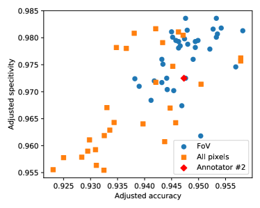
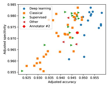
In Figure 6 we have plotted the distribution of algorithms and evaluation methodologies in the adjusted accuracy-specificity plane. The plot shows that after eliminating the bias, the algorithms evaluated with all pixels have lower accuracy and specificity scores than those evaluated with the FoV mask. The independent two-sample t-test shows that the difference is statistically significant with a p-value of . The reason for this surprising phenomenon is that using all pixels to evaluate less effective techniques results in performance scores comparable to or even higher than those of more effective techniques evaluated under the FoV mask, and this brings publicity to less effective approaches.
Finally, we compare the performances of the methods by their operating principles. We have introduced 4 categories: deep learning, classical (thresholding, filtering, morphology, region growing), supervised (feature extraction and supervised machine learning, but not deep learning), and others (dominantly graph-cut based segmentation techniques). The results presented in Figure 6 show that deep learning techniques increase the accuracy by almost 1% compared to the best performing classical and supervised techniques.
4.3 A remark on the evaluation of deep learning techniques
From a development perspective, there is an important difference between heuristic image processing pipelines and highly flexible deep learning solutions that calls into question the suitability of current evaluation methodologies in the field. Unlike the heuristic improvement of conventional image processing pipelines, the tuning of hyperparameters in deep neural networks is relatively straightforward (automated in many cases), which increases the risk of overfitting when the performance scores measured on the test set drive the tuning of the network.
Although this could be prevented by using the training images of DRIVE for both training the weights in the network and tuning the network structure, we found evidence that some results are clearly overfitted to the test set: Both (Li et al., 2016) and (Liskowski and Krawiec, 2016) optimize the network size and hyperparameters on the test images. Despite the obvious overfitting, we did not discard these results for two reasons. First, all other papers using deep learning declare the network structures and the hyperparameters. None of the authors describe how the network was derived from the training data, which risks the overfitting of the network structure to the test images. On the other hand, there is no doubt that deep learning techniques achieve better results than classical approaches. Although some papers may have reported too optimistic scores due to overfitting to the test images, they clearly dominate the field.
Consequently, the development and evaluation of deep learning solutions for retinal vessel segmentation should follow the standards of the deep learning literature by using 3 sets of images (Larochelle et al., 2009): one to train the weights in the network, another to tune the network structure and a final one to test the performance of the optimised network. However, since DRIVE specifies only 2 subsets and further splitting of the training set (20 images) would lead to a nearly insufficient number of images for deep learning, a larger set of images should become the standard in this field.
4.4 Limitations
The analysis we carried out has numerous limitations. Despite the systematic search for influential papers, the selected group may provide a biassed representation of the field and the results of the selection process may change over time as the number of citations changes.
The consistency tests for aggregated figures tolerate greater deviation from the hypotheses than do the image level tests. This inherent imbalance in the rigour of the tests implies that some papers that passed the consistency test with aggregated scores might have failed if the authors had reported image level scores.
The adjusted scores have some numerical uncertainty. Although the estimated errors are small, the improved ranking is also uncertain to this degree.
We have focused primarily on the comparability of the reported performance scores. However, higher performance is not the only goal in science. If some methods are easier to understand, maintain, adapt, or are more efficient in terms of runtime, they are still valuable contributions to science. Therefore, the improved ranking does not devalue the contributions of any paper, as all papers provide insights into the capabilities of the implemented approaches.
5 Summary and Conclusions
In this study, we investigated the coherence of reported performance scores in the segmentation of vessels in retinal images. We collected 100 influential papers reporting accuracy, sensitivity, and specificity for the publicly available data set DRIVE. Based on textual references to two corner cases of evaluation methodologies (evaluation under the FoV mask or using all pixels of the images), we developed numerical methods to test the consistency of the reported scores with the two assumed corner cases (subsections 3.3.1, 3.4.1). Based on results of consistency tests, we attempted to remove bias and make the scores comparable to create a new baseline ranking (Section 3.5). Section 4 summarizes various findings and insights and also discusses the limitations of our analysis. The insights clearly show that there is no consensus in the field on the evaluation methodology. However, in most of the papers, including reviews of the field, the rankings and the objective evaluation of operating principles are biassed by the direct comparison of non-comparable figures. Based on the papers we selected and the adjustment we implemented, the current state of the art accuracy is 0.9582 (evaluated in the FoV region), which is about 1.1% higher than the performance of annotator #2. Despite the limitations of our method, we believe that the adjusted ranking in Table 4 provides a more realistic view of the state of the art than any ranking based on the direct comparison of reported figures.
The findings have numerous implications regarding the suitability and potential improvements of data sets, evaluation methodologies and reporting standards in the field:
-
•
A novel data set that takes into account the changing requirements of the field is desirable - potentially, this could emerge as a curated fusion of existing vessel segmentation data sets that provides predefined training, test and validation subsets for the reliable evaluation of deep learning techniques, and the sizes of the subsets should be based on well-established principles (Guyon et al., 1998).
-
•
The published average scores on DRIVE usually differ in the 3th-4th digits. Since these are the averages of only 20 image level scores, one can assume a relatively large variance, which makes the rankings ambigious. To investigate whether there were statistically significant improvements, the authors should provide image level figures at least as supplementary material and explicitly report more details about the evaluation methodology (e.g., the region they use to calculate the scores).
-
•
Authors should report the Dice score (Eelbode et al., 2020), , which is a commonly accepted measure of segmentation performance. Since is inherently free of the number of true negatives, the bias we study in this paper is naturally eliminated. Treating retinal vessel segmentation as a pixelwise binary classification problem, the AUC score (the standard performance measure for binary classification in machine learning) provides good insight into the trade-off between the sensitivity and specificity of segmentation algorithms - if applicable (the segmentation is based on pixelwise vesselness probabilities), authors should report AUC scores.
-
•
Maximizing some pixelwise performance measures of segmentation does not necessarily improve clinical applications. For example, an algorithm that provides an average accuracy of 0.95 with a small standard deviation may lead to a more reliable grading of disease severity than an algorithm with an average accuracy of 0.96 and a huge standard deviation, which means that it fails under certain conditions. Consequently, the evaluation of vessel segmentation methods should be more closely linked to clinical applications.
The numerical techniques we have developed can be easily adapted to other problems where similar methodological flaws may arise. To allow full reproducibility and further analysis, all raw data, the implementation of the analysis and all results are shared in the GitHub repository www.github.com/gykovacs/retinal_vessel_segmentation.
Acknowledgments
György Kovács would like to thank the support of the initiative 1LU-51P-4E. On behalf of Attila Fazekas, this work was supported by the construction EFOP-3.6.3-VEKOP-16-2017-00002. The project was supported by the European Union, co-financed by the European Social Fund.
References
- Abramoff et al. (2010) Abramoff, M., Garvin, M., Sonka, M., 2010. Retinal imaging and image analysis. Biomedical Engineering, IEEE Reviews in 3, 169 – 208. doi:10.1109/RBME.2010.2084567.
- Adapa et al. (2020) Adapa, D., Joseph Raj, A.N., Alisetti, S.N., Zhuang, Z., K., G., Naik, G., 2020. A supervised blood vessel segmentation technique for digital fundus images using zernike moment based features. PLOS ONE 15, 1–23. doi:10.1371/journal.pone.0229831.
- Almotiri et al. (2018) Almotiri, J., Elleithy, K., Elleithy, A., 2018. Retinal vessels segmentation techniques and algorithms: A survey. Applied Sciences 8. doi:10.3390/app8020155.
- Alom et al. (2019) Alom, M.Z., Yakopcic, C., Hasan, M., Taha, T., Asari, V., 2019. Recurrent residual u-net for medical image segmentation. Journal of Medical Imaging 6. doi:10.1117/1.JMI.6.1.014006.
- Anzalone et al. (2008) Anzalone, A., Bizzarri, F., Parodi, M., Storace, M., 2008. A modular supervised algorithm for vessel segmentation in red-free retinal images. Comput. Biol. Med. 38, 913–922. doi:10.1016/j.compbiomed.2008.05.006.
- Atli and Gedik (2021) Atli, I., Gedik, O.S., 2021. Sine-net: A fully convolutional deep learning architecture for retinal blood vessel segmentation. Engineering Science and Technology, an International Journal 24, 271–283. doi:https://doi.org/10.1016/j.jestch.2020.07.008.
- Azzopardi et al. (2015) Azzopardi, G., Strisciuglio, N., Vento, M., Petkov, N., 2015. Trainable cosfire filters for vessel delineation with application to retinal images. Medical Image Analysis 19, 46–57. doi:https://doi.org/10.1016/j.media.2014.08.002.
- Barkana et al. (2017) Barkana, B., Saricicek, I., Yildirim, B., 2017. Performance analysis of descriptive statistical features in retinal vessel segmentation via fuzzy logic, ann, svm, and classifier fusion. Knowledge-Based Systems 118. doi:10.1016/j.knosys.2016.11.022.
- Besenczi et al. (2016) Besenczi, R., Tóth, J., Hajdu, A., 2016. A review on automatic analysis techniques for color fundus photographs. Computational and Structural Biotechnology Journal 14, 371–384. doi:10.1016/j.csbj.2016.10.001.
- Bharkad (2017) Bharkad, S., 2017. Automatic segmentation of blood vessels in retinal image using morphological filters, in: Proceedings of the 6th International Conference on Software and Computer Applications - ICSCA17, ACM Press. doi:10.1145/3056662.3056710.
- Brancati et al. (2018) Brancati, N., Frucci, M., Gragnaniello, D., Riccio, D., 2018. Retinal Vessels Segmentation Based on a Convolutional Neural Network. pp. 119–126. doi:10.1007/978-3-319-75193-1_15.
- Budai et al. (2013) Budai, A., Bock, R., Maier, A., Hornegger, J., Michelson, G., 2013. Robust vessel segmentation in fundus images. International Journal of Biomedical Imaging 2013.
- Cetinkaya and Duran (2020) Cetinkaya, M.B., Duran, H., 2020. A detailed and comparative work for retinal vessel segmentation based on the most effective heuristic approaches. Biomedical Engineering / Biomedizinische Technik 0. doi:10.1515/bmt-2020-0089.
- Chalakkal and Abdulla (2017) Chalakkal, R.J., Abdulla, W., 2017. Automatic segmentation of retinal vasculature, in: 2017 IEEE International Conference on Acoustics, Speech and Signal Processing (ICASSP), pp. 886–890. doi:10.1109/ICASSP.2017.7952283.
- Cheng et al. (2014) Cheng, E., Du, L., Wu, Y., Zhu, Y., Megalooikonomou, V., Ling, H., 2014. Discriminative vessel segmentation in retinal images by fusing context-aware hybrid features. Machine Vision and Applications 25, 1779–1792. doi:10.1007/s00138-014-0638-x.
- lui Cheung et al. (2012) lui Cheung, C.Y., Ikram, M.K., Sabanayagam, C., Wong, T.Y., 2012. Retinal microvasculature as a model to study the manifestations of hypertension. Hypertension 60, 1094–1103. doi:10.1161/hypertensionaha.111.189142.
- Dai et al. (2015) Dai, P., Luo, H., Sheng, H., Zhao, Y., Li, L., Wu, J., Zhao, Y., Suzuki, K., 2015. A new approach to segment both main and peripheral retinal vessels based on gray-voting and gaussian mixture model. PLOS ONE 10, 1–22. doi:10.1371/journal.pone.0127748.
- Dasgupta and Singh (2017) Dasgupta, A., Singh, S., 2017. A fully convolutional neural network based structured prediction approach towards the retinal vessel segmentation, in: 2017 IEEE 14th International Symposium on Biomedical Imaging (ISBI 2017), pp. 248–251. doi:10.1109/ISBI.2017.7950512.
- Dash and Bhoi (2018) Dash, J., Bhoi, N., 2018. An unsupervised approach for extraction of blood vessels from fundus images. Journal of Digital Imaging 31, 857–868.
- Dash et al. (2020) Dash, J., Priyadarsan, P., Nilamani, B., 2020. Retinal blood vessel extraction from fundus images using enhancement filtering and clustering. ELCVIA: electronic letters on computer vision and image analysis 19, 38–52.
- Dizdaroglu et al. (2012) Dizdaroglu, B., Cansizoglu, E., Kalpathy-Cramer, J., Keck, K., Chiang, M., Erdoğmuş, D., 2012. Level sets for retinal vasculature segmentation using seeds from ridges and edges from phase maps. 2012 IEEE International Workshop on Machine Learning for Signal Processing , 1–6.
- Eelbode et al. (2020) Eelbode, T., Bertels, J., Berman, M., Vandermeulen, D., Maes, F., Bisschops, R., Blaschko, M.B., 2020. Optimization for medical image segmentation: Theory and practice when evaluating with dice score or jaccard index. IEEE Transactions on Medical Imaging 39, 3679–3690. doi:10.1109/TMI.2020.3002417.
- Emary et al. (2014) Emary, E., Zawbaa, H., Hassanien, A.E., Schaefer, G., Azar, A., 2014. Retinal blood vessel segmentation using bee colony optimisation and pattern search. doi:10.1109/IJCNN.2014.6889856.
- Escorcia-Gutierrez et al. (2020) Escorcia-Gutierrez, J., Torrents-Barrena, J., Gamarra, M., Romero-Aroca, P., Valls, A., Puig, D., 2020. Convexity shape constraints for retinal blood vessel segmentation and foveal avascular zone detection. Computers in Biology and Medicine 127, 104049. doi:https://doi.org/10.1016/j.compbiomed.2020.104049.
- Fan et al. (2017) Fan, Z., Lu, J., Li, W., Wei, C., Huang, H., Cai, X., Chen, X., 2017. A hierarchical image matting model for blood vessel segmentation in fundus images. arXiv:1701.00892.
- Fathi and Naghsh-Nilchi (2013) Fathi, A., Naghsh-Nilchi, A.R., 2013. Automatic wavelet-based retinal blood vessels segmentation and vessel diameter estimation. Biomedical Signal Processing and Control 8, 71 -- 80. doi:https://doi.org/10.1016/j.bspc.2012.05.005.
- Fraz et al. (2012a) Fraz, M., Barman, S., Remagnino, P., Hoppe, A., Basit, A., Uyyanonvara, B., Rudnicka, A., Owen, C., 2012a. An approach to localize the retinal blood vessels using bit planes and centerline detection. Computer Methods and Programs in Biomedicine 108, 600 -- 616. doi:https://doi.org/10.1016/j.cmpb.2011.08.009.
- Fraz et al. (2012b) Fraz, M., Remagnino, P., Hoppe, A., Uyyanonvara, B., Rudnicka, A., Owen, C., Barman, S., 2012b. Blood vessel segmentation methodologies in retinal images - a survey. Computer methods and programs in biomedicine 108, 407--33. doi:10.1016/j.cmpb.2012.03.009.
- Fraz et al. (2012c) Fraz, M.M., Remagnino, P., Hoppe, A., Uyyanonvara, B., Rudnicka, A.R., Owen, C.G., Barman, S.A., 2012c. An ensemble classification-based approach applied to retinal blood vessel segmentation. IEEE transactions on bio-medical engineering 59, 2538—2548. doi:10.1109/tbme.2012.2205687.
- Frucci et al. (2017) Frucci, M., Riccio, D., Sanniti di Baja, G., Serino, L., 2017. Direction-based segmentation of retinal blood vessels, in: Beltrán-Castañón, C., Nyström, I., Famili, F. (Eds.), Progress in Pattern Recognition, Image Analysis, Computer Vision, and Applications, Springer International Publishing, Cham. pp. 1--9.
- Frucci et al. (2016) Frucci, M., Riccio, D., di Baja, G.S., Serino, L., 2016. Severe: Segmenting vessels in retina images. Pattern Recognition Letters 82, 162--169. doi:10.1016/j.patrec.2015.07.002.
- Fu et al. (2018) Fu, D., Liu, Y., Huang, Z., 2018. A review of retinal vessel segmentation and artery/vein classification, in: Jia, Y., Du, J., Zhang, W. (Eds.), Proceedings of 2017 Chinese Intelligent Systems Conference, Springer Singapore, Singapore. pp. 727--737.
- GeethaRamani and Bal/an (2016) GeethaRamani, R., Bal/an, L., 2016. Retinal blood vessel segmentation employing image processing and data mining techniques for computerized retinal image analysis. Biocybernetics and Biomedical Engineering 36, 102 -- 118. doi:https://doi.org/10.1016/j.bbe.2015.06.004.
- Guyon et al. (1998) Guyon, I., Makhoul, J., Schwartz, R.M., Vapnik, V., 1998. What size test set gives good error rate estimates?. IEEE Trans. Pattern Anal. Mach. Intell. 20, 52--64. URL: http://dblp.uni-trier.de/db/journals/pami/pami20.html#GuyonMSV98.
- Hanley and Mcneil (1982) Hanley, J., Mcneil, B., 1982. The meaning and use of the area under a receiver operating characteristic (roc) curve. Radiology 143, 29--36. doi:10.1148/radiology.143.1.7063747.
- Hassanien (2018) Hassanien, A.E., 2018. Retinal fundus vasculature multilevel-segmentation using whale optimization algorithm. Signal, Image and Video Processing 12. doi:10.1007/s11760-017-1154-z.
- Hoover et al. (2000) Hoover, A.D., Kouznetsova, V., Goldbaum, M., 2000. Locating blood vessels in retinal images by piecewise threshold probing of a matched filter response. IEEE Transactions on Medical Imaging 19, 203--210. doi:10.1109/42.845178.
- Hu et al. (2018) Hu, K., Zhang, Z., Niu, X., Zhang, Y., Cao, C., Xiao, F., Gao, X., 2018. Retinal vessel segmentation of color fundus images using multiscale convolutional neural network with an improved cross-entropy loss function. Neurocomputing 309, 179 -- 191. doi:https://doi.org/10.1016/j.neucom.2018.05.011.
- Imani et al. (2015) Imani, E., Javidi, M., Pourreza, H.R., 2015. Improvement of retinal blood vessel detection using morphological component analysis. Computer Methods and Programs in Biomedicine 118, 263 -- 279. doi:https://doi.org/10.1016/j.cmpb.2015.01.004.
- Isavand Rahmani et al. (2020) Isavand Rahmani, A., Akbari, H., Saraf Esmaili, S., 2020. Retinal blood vessel segmentation using gabor filter and morphological reconstruction. Signal Processing and Renewable Energy 4, 77--88.
- Javidi et al. (2017) Javidi, M., Pourreza, H.R., Harati, A., 2017. Vessel segmentation and microaneurysm detection using discriminative dictionary learning and sparse representation. Computer Methods and Programs in Biomedicine 139, 93--108. doi:https://doi.org/10.1016/j.cmpb.2016.10.015.
- Jebaseeli et al. (2019) Jebaseeli, T., Chelladurai, A., Peter, J., 2019. Retinal blood vessel segmentation from diabetic retinopathy images using tandem pcnn model and deep learning based svm. Optik 199, 163328. doi:10.1016/j.ijleo.2019.163328.
- Jiang and Mojon (2003) Jiang, X., Mojon, D., 2003. Adaptive local thresholding by verification-based multithreshold probing with application to vessel detection in retinal images. IEEE Trans. Pattern Anal. Mach. Intell. 25, 131–137. doi:10.1109/TPAMI.2003.1159954.
- Jiang et al. (2019) Jiang, Y., Zhang, H., Tan, N., Chen, L., 2019. Automatic retinal blood vessel segmentation based on fully convolutional neural networks. Symmetry 11, 1112. doi:10.3390/sym11091112.
- Jin et al. (2019) Jin, Q., Meng, Z.P., Pham, T., Chen, Q., Wei, L., Su, R., 2019. Dunet: A deformable network for retinal vessel segmentation. Knowl. Based Syst. 178, 149--162.
- Kaur and Mittal (2017) Kaur, J., Mittal, D., 2017. A generalized method for the detection of vascular structure in pathological retinal images. Biocybernetics and Biomedical Engineering 37. doi:10.1016/j.bbe.2016.09.002.
- Khan et al. (2018) Khan, K.B., Khaliq, A.A., Jalil, A., Iftikhar, M.A., Ullah, N., Aziz, M.W., Ullah, K., Shahid, M., 2018. A review of retinal blood vessels extraction techniques: challenges, taxonomy, and future trends. Pattern Analysis and Applications 22, 767--802. doi:10.1007/s10044-018-0754-8.
- Khan et al. (2016) Khan, M., Soomro, T., Khan, T., Bailey, D., Gao, J., Mir, N., 2016. Automatic retinal vessel extraction algorithm based on contrast-sensitive schemes, pp. 1--5. doi:10.1109/IVCNZ.2016.7804441.
- Kovács and Hajdu (2016) Kovács, G., Hajdu, A., 2016. A self-calibrating approach for the segmentation of retinal vessels by template matching and contour reconstruction. Medical Image Analysis 29(4), 24--46. doi:10.1016/j.media.2015.12.003.
- Kumar et al. (2016) Kumar, D., Pramanik, A., Kar, S.S., Maity, S.P., 2016. Retinal blood vessel segmentation using matched filter and laplacian of gaussian, in: 2016 International Conference on Signal Processing and Communications (SPCOM), pp. 1--5. doi:10.1109/SPCOM.2016.7746666.
- Kumar et al. (2020) Kumar, K., Samal, D., Suraj, 2020. Automated retinal vessel segmentation based on morphological preprocessing and 2d-gabor wavelets, in: Pati, B., Panigrahi, C.R., Buyya, R., Li, K.C. (Eds.), Advanced Computing and Intelligent Engineering, Springer Singapore, Singapore. pp. 411--423.
- Larochelle et al. (2009) Larochelle, H., Bengio, Y., Louradour, J., Lamblin, P., 2009. Exploring strategies for training deep neural networks. Journal of Machine Learning Research 10, 1--40.
- Li et al. (2016) Li, Q., Feng, B., Xie, L., Liang, P., Zhang, H., Wang, T., 2016. A cross-modality learning approach for vessel segmentation in retinal images. IEEE Transactions on Medical Imaging 35, 109--118. doi:10.1109/TMI.2015.2457891.
- Liskowski and Krawiec (2016) Liskowski, P., Krawiec, K., 2016. Segmenting retinal blood vessels with deep neural networks. IEEE Transactions on Medical Imaging 35, 2369--2380. doi:10.1109/TMI.2016.2546227.
- Long et al. (2020) Long, S., Chen, J., Hu, A., Liu, H., Chen, Z., Zheng, D., 2020. Microaneurysms detection in color fundus images using machine learning based on directional local contrast. BioMedical Engineering OnLine 19. doi:10.1186/s12938-020-00766-3.
- Lupaşcu et al. (2010) Lupaşcu, C.A., Tegolo, D., Trucco, E., 2010. Fabc: Retinal vessel segmentation using adaboost. Trans. Info. Tech. Biomed. 14, 1267–1274. doi:10.1109/TITB.2010.2052282.
- Lupascu and Tegolo (2016) Lupascu, C.A., Tegolo, D., 2016. A multiscale approach to automatic and unsupervised retinal vessel segmentation using self-organizing maps, in: Proceedings of the 17th International Conference on Computer Systems and Technologies 2016, ACM. doi:10.1145/2983468.2983478.
- Maier-Hein et al. (2018) Maier-Hein, L., Eisenmann, M., Reinke, A., Onogur, S., Stankovic, M., Scholz, P., Arbel, T., Bogunovic, H., Bradley, A.P., Carass, A., Feldmann, C., Frangi, A.F., Full, P.M., van Ginneken, B., Hanbury, A., Honauer, K., Kozubek, M., Landman, B.A., März, K., Maier, O., Maier-Hein, K., Menze, B.H., Müller, H., Neher, P.F., Niessen, W., Rajpoot, N., Sharp, G.C., Sirinukunwattana, K., Speidel, S., Stock, C., Stoyanov, D., Taha, A.A., van der Sommen, F., Wang, C.W., Weber, M.A., Zheng, G., Jannin, P., Kopp-Schneider, A., 2018. Why rankings of biomedical image analysis competitions should be interpreted with care. Nature Communications 9. URL: https://doi.org/10.1038/s41467-018-07619-7, doi:10.1038/s41467-018-07619-7.
- Mapayi et al. (2015) Mapayi, T., Viriri, S., Tapamo, J.R., 2015. Adaptive thresholding technique for retinal vessel segmentation based on glcm-energy information. Comput. Math. Methods Medicine 2015, 597475:1--597475:11.
- Marin et al. (2011) Marin, D., Aquino, A., Gegúndez-Arias, M.E., Bravo, J.M., 2011. A new supervised method for blood vessel segmentation in retinal images by using gray-level and moment invariants-based features. IEEE Transactions on Medical Imaging 30, 146--158.
- Martinez-Perez et al. (2007) Martinez-Perez, M.E., Hughes, A.D., Thom, S.A., Bharath, A.A., Parker, K.H., 2007. Segmentation of blood vessels from red-free and fluorescein retinal images. Medical image analysis 11, 47—61. doi:10.1016/j.media.2006.11.004.
- Melinscak et al. (2015) Melinscak, M., Prentasic, P., Loncaric, S., 2015. Retinal vessel segmentation using deep neural networks. VISAPP 2015 - 10th International Conference on Computer Vision Theory and Applications; VISIGRAPP, Proceedings 1, 577--582. doi:10.5220/0005313005770582.
- Memari et al. (2017) Memari, N., Ramli, A.R., Bin Saripan, M.I., Mashohor, S., Moghbel, M., 2017. Supervised retinal vessel segmentation from color fundus images based on matched filtering and adaboost classifier. PLOS ONE 12, 1--35. doi:10.1371/journal.pone.0188939.
- Mendonca and Campilho (2006) Mendonca, A.M., Campilho, A.C., 2006. Segmentation of retinal blood vessels by combining the detection of centerlines and morphological reconstruction. IEEE Trans. Med. Imaging 25, 1200--1213.
- Meng et al. (2015) Meng, X., Yin, Y., Yang, G., Han, Z., Yan, X., 2015. A framework for retinal vasculature segmentation based on matched filters. Biomedical engineering online 14, 94. doi:10.1186/s12938-015-0089-2.
- Miri and Mahloojifar (2010) Miri, M.S., Mahloojifar, A., 2010. Retinal image analysis using curvelet transform and multistructure elements morphology by reconstruction. IEEE transactions on bio-medical engineering 58, 1183--92. doi:10.1109/TBME.2010.2097599.
- Mo and Zhang (2017) Mo, J., Zhang, L., 2017. Multi-level deep supervised networks for retinal vessel segmentation. International journal of computer assisted radiology and surgery 12. doi:10.1007/s11548-017-1619-0.
- Moccia et al. (2018) Moccia, S., De Momi, E., El Hadji, S., Mattos, L.S., 2018. Blood vessel segmentation algorithms — review of methods, datasets and evaluation metrics. Computer Methods and Programs in Biomedicine 158, 71--91. doi:https://doi.org/10.1016/j.cmpb.2018.02.001.
- Moghimirad et al. (2011) Moghimirad, E., Rezatofighi, H., Soltanian-Zadeh, H., 2011. Retinal vessel segmentation using a multi-scale medialness function. Computers in biology and medicine 42, 50--60. doi:10.1016/j.compbiomed.2011.10.008.
- Mookiah et al. (2021) Mookiah, M.R.K., Hogg, S., MacGillivray, T.J., Prathiba, V., Pradeepa, R., Mohan, V., Anjana, R.M., Doney, A.S., Palmer, C.N., Trucco, E., 2021. A review of machine learning methods for retinal blood vessel segmentation and artery/vein classification. Medical Image Analysis 68, 101905. doi:https://doi.org/10.1016/j.media.2020.101905.
- Na et al. (2018) Na, T., Xie, J., Zhao, Y., Zhao, Y., Liu, Y., Wang, Y., Liu, J., 2018. Retinal vascular segmentation using superpixel-based line operator and its application to vascular topology estimation. Medical Physics 45, 3132--3146. doi:10.1002/mp.12953.
- Narkthewan and Maneerat (2019) Narkthewan, A., Maneerat, N., 2019. Retina blood vessel detection for diabetic retinopathy diagnosis, in: Proceedings of the 2019 9th International Conference on Biomedical Engineering and Technology, Association for Computing Machinery, New York, NY, USA. p. 149–152. URL: https://doi.org/10.1145/3326172.3326203.
- Nazari and Pourghassem (2013) Nazari, P., Pourghassem, H., 2013. An automated vessel segmentation algorithm in retinal images using 2d gabor wavelet, in: 2013 8th Iranian Conference on Machine Vision and Image Processing (MVIP), IEEE. doi:10.1109/iranianmvip.2013.6779967.
- Ngo and Han (2017) Ngo, L., Han, J.., 2017. Multi-level deep neural network for efficient segmentation of blood vessels in fundus images. Electronics Letters 53, 1096--1098. doi:10.1049/el.2017.2066.
- Niemeijer et al. (2004) Niemeijer, M., Staal, J., van Ginneken, B., Loog, M., Abramoff, M.D., 2004. Comparative study of retinal vessel segmentation methods on a new publicly available database, in: Fitzpatrick, J.M., Sonka, M. (Eds.), Medical Imaging 2004: Image Processing, International Society for Optics and Photonics. SPIE. pp. 648 -- 656. doi:10.1117/12.535349.
- Noh et al. (2019) Noh, K.J., Park, S.J., Lee, S., 2019. Scale-space approximated convolutional neural networks for retinal vessel segmentation. Computer Methods and Programs in Biomedicine 178, 237--246. doi:https://doi.org/10.1016/j.cmpb.2019.06.030.
- Odstrcilik et al. (2013) Odstrcilik, J., Kolar, R., Budai, A., Hornegger, J., Jan, J., Gazarek, J., Kubena, T., Cernosek, P., Svoboda, O., Angelopoulou, E., 2013. Retinal vessel segmentation by improved matched filtering: evaluation on a new high-resolution fundus image database. IET Image Processing 7, 373--383. doi:10.1049/iet-ipr.2012.0455.
- Palanivel et al. (2020) Palanivel, D.A., Natarajan, S., Gopalakrishnan, S., 2020. Retinal vessel segmentation using multifractal characterization. Applied Soft Computing 94, 106439. doi:https://doi.org/10.1016/j.asoc.2020.106439.
- Panda et al. (2016) Panda, R., Puhan, N.B., Panda, G., 2016. New binary hausdorff symmetry measure based seeded region growing for retinal vessel segmentation. Biocybernetics and Biomedical Engineering 36, 119--129.
- Pandey et al. (2017) Pandey, D., Yin, X., Wang, H., Zhang, Y., 2017. Accurate vessel segmentation using maximum entropy incorporating line detection and phase-preserving denoising. Computer Vision and Image Understanding 155, 162 -- 172. doi:https://doi.org/10.1016/j.cviu.2016.12.005.
- Park et al. (2020) Park, K.B., Choi, S.H., Lee, J.Y., 2020. M-gan: Retinal blood vessel segmentation by balancing losses through stacked deep fully convolutional networks. IEEE Access 8, 146308--146322. doi:10.1109/ACCESS.2020.3015108.
- Porwal et al. (2020) Porwal, P., Pachade, S., Kokare, M., Deshmukh, G., et al., 2020. IDRiD: Diabetic retinopathy – segmentation and grading challenge. Medical Image Analysis 59, 101561. URL: https://doi.org/10.1016/j.media.2019.101561, doi:10.1016/j.media.2019.101561.
- Rahebi and Hardalaç (2014) Rahebi, J., Hardalaç, F., 2014. Retinal blood vessel segmentation with neural network by using gray-level co-occurrence matrix-based features. Journal of medical systems 38, 85. doi:10.1007/s10916-014-0085-2.
- Rezaee et al. (2017) Rezaee, K., Haddadnia, J., Tashk, A., 2017. Optimized clinical segmentation of retinal blood vessels by using combination of adaptive filtering, fuzzy entropy and skeletonization. Applied Soft Computing 52, 937 -- 951. doi:https://doi.org/10.1016/j.asoc.2016.09.033.
- Ricci and Perfetti (2007) Ricci, E., Perfetti, R., 2007. Retinal blood vessel segmentation using line operators and support vector classification. IEEE Transactions on Medical Imaging 26, 1357--1365.
- Roychowdhury et al. (2015) Roychowdhury, S., Koozekanani, D.D., Parhi, K.K., 2015. Iterative vessel segmentation of fundus images. IEEE Transactions on Biomedical Engineering 62, 1738--1749. doi:10.1109/TBME.2015.2403295.
- Salazar et al. (2014) Salazar, A., Kaba, D., Li, Y., Liu, X., 2014. Segmentation of blood vessels and optic disc in retinal images. IEEE journal of biomedical and health informatics 18. doi:10.1109/JBHI.2014.2302749.
- Saleh et al. (2011) Saleh, D., Eswaran, C., Mueen, A., 2011. An automated blood vessel segmentation algorithm using histogram equalization and automatic threshold selection. Journal of digital imaging : the official journal of the Society for Computer Applications in Radiology 24, 564--72. doi:10.1007/s10278-010-9302-9.
- Samuel and Veeramalai (2019) Samuel, P.M., Veeramalai, T., 2019. Multilevel and multiscale deep neural network for retinal blood vessel segmentation. Symmetry 11, 946.
- Saroj et al. (2020) Saroj, S.K., Kumar, R., Singh, N.P., 2020. Fréchet pdf based matched filter approach for retinal blood vessels segmentation. Computer methods and programs in biomedicine 194, 105490. doi:10.1016/j.cmpb.2020.105490.
- Shah et al. (2017) Shah, S., Tang, T.B., Faye, I., Laude, A., 2017. Blood vessel segmentation in color fundus images based on regional and hessian features. Graefe’s Archive for Clinical and Experimental Ophthalmology 255. doi:10.1007/s00417-017-3677-y.
- Shukla et al. (2020) Shukla, A.K., Pandey, R.K., Pachori, R.B., 2020. A fractional filter based efficient algorithm for retinal blood vessel segmentation. Biomedical Signal Processing and Control 59, 101883. doi:https://doi.org/10.1016/j.bspc.2020.101883.
- Singh et al. (2020) Singh, N., Bansal, D., Nagpal, D., 2020. Deep learning based retinal vessel segmentation: a review. Advances in Mathematics: Scientific Journal 9, 3827--3837. doi:10.37418/amsj.9.6.62.
- Singh and Srivastava (2016) Singh, N.P., Srivastava, R., 2016. Retinal blood vessels segmentation by using gumbel probability distribution function based matched filter. Computer Methods and Programs in Biomedicine 129, 40 -- 50. doi:https://doi.org/10.1016/j.cmpb.2016.03.001.
- Singh and Srivastava (2017) Singh, N.P., Srivastava, R., 2017. Weibull probability distribution function-based matched filter approach for retinal blood vessels segmentation, in: Sahana, S.K., Saha, S.K. (Eds.), Advances in Computational Intelligence, Springer Singapore, Singapore. pp. 427--437.
- Song and Lee (2017) Song, J., Lee, B., 2017. Development of automatic retinal vessel segmentation method in fundus images via convolutional neural networks, in: 2017 39th Annual International Conference of the IEEE Engineering in Medicine and Biology Society (EMBC), pp. 681--684. doi:10.1109/EMBC.2017.8036916.
- Soomro et al. (2017) Soomro, T., Khan, M., Gao, J., Khan, T., Khan, M., Paul, M., 2017. Contrast normalization steps for increased sensitivity of a retinal image segmentation method. Signal Image and Video Processing doi:10.1007/s11760-017-1114-7.
- Soomro et al. (2018) Soomro, T., Khan, T., Khan, M., Gao, J., Paul, M., Zheng, L., 2018. Impact of ica-based image enhancement technique on retinal blood vessels segmentation. IEEE Access PP. doi:10.1109/ACCESS.2018.2794463.
- Soomro et al. (2019) Soomro, T.A., Afifi, A.J., Gao, J., Hellwich, O., Zheng, L., Paul, M., 2019. Strided fully convolutional neural network for boosting the sensitivity of retinal blood vessels segmentation. Expert Systems with Applications 134, 36 -- 52. doi:https://doi.org/10.1016/j.eswa.2019.05.029.
- Sreejini and Govindan (2015) Sreejini, K., Govindan, V., 2015. Improved multiscale matched filter for retina vessel segmentation using pso algorithm. Egyptian Informatics Journal 16, 253--260. doi:https://doi.org/10.1016/j.eij.2015.06.004.
- Srinidhi et al. (2017) Srinidhi, C.L., Aparna, P., Rajan, J., 2017. Recent advancements in retinal vessel segmentation. Journal of Medical Systems 41. doi:10.1007/s10916-017-0719-2.
- Staal et al. (2004) Staal, J., Abramoff, M., Niemeijer, M., Viergever, M., Ginneken, B., 2004. Ridge-based vessel segmentation in color images of the retina. IEEE transactions on medical imaging 23, 501--9. doi:10.1109/TMI.2004.825627.
- Strisciuglio et al. (2015) Strisciuglio, N., Azzopardi, G., Vento, M., Petkov, N., 2015. Unsupervised delineation of the vessel tree in retinal fundus images. doi:10.1201/b19241-26.
- Strisciuglio et al. (2016) Strisciuglio, N., Azzopardi, G., Vento, M., Petkov, N., 2016. Supervised vessel delineation in retinal fundus images with the automatic selection of b-COSFIRE filters. Machine Vision and Applications 27, 1137--1149. doi:10.1007/s00138-016-0781-7.
- Tamim et al. (2020) Tamim, N., Elshrkawey, M., Abdel Azim, G., Nassar, H., 2020. Retinal blood vessel segmentation using hybrid features and multi-layer perceptron neural networks. Symmetry 12. doi:10.3390/sym12060894.
- Tang et al. (2017) Tang, Z., Zhang, J., Gui, W., 2017. Selective search and intensity context based retina vessel image segmentation. Journal of Medical Systems 41. doi:10.1007/s10916-017-0696-5.
- Thangaraj et al. (2018) Thangaraj, S., Periyasamy, V., Balaji, R., 2018. Retinal vessel segmentation using neural network. IET Image Processing 12, 669--678. doi:10.1049/iet-ipr.2017.0284.
- Trucco et al. (2019) Trucco, E., MacGillivray, T., Xu, Y. (Eds.), 2019. Computational Retinal Image Analysis. Elsevier. doi:10.1016/c2018-0-00865-8.
- Vandewiele et al. (2021) Vandewiele, G., Dehaene, I., Kovács, G., Sterckx, L., Janssens, O., Ongenae, F., De Backere, F., De Turck, F., Roelens, K., Decruyenaere, J., Van Hoecke, S., Demeester, T., 2021. Overly optimistic prediction results on imbalanced data: a case study of flaws and benefits when applying over-sampling. Artificial Intelligence in Medicine 111, 101987. doi:10.1016/j.artmed.2020.101987.
- Villalobos-Castaldi et al. (2010) Villalobos-Castaldi, F.M., Riverón, E.M.F., Fernández, L., 2010. A fast, efficient and automated method to extract vessels from fundus images. Journal of Visualization 13, 263--270.
- Waheed et al. (2015) Waheed, A., Akram, M., Khalid, S., Waheed, Z., Khan, M., Shaukat, A., 2015. Hybrid features and mediods classification based robust segmentation of blood vessels. Journal of Medical Systems 39. doi:10.1007/s10916-015-0316-1.
- Wang et al. (2015) Wang, S., Yin, Y., Cao, G., Wei, B., Zheng, Y., Yang, G., 2015. Hierarchical retinal blood vessel segmentation based on feature and ensemble learning. Neurocomputing 149, 708 -- 717. doi:https://doi.org/10.1016/j.neucom.2014.07.059.
- Wankhede and Khanchandani (2015) Wankhede, P.R., Khanchandani, K.B., 2015. Retinal blood vessel segmentation using graph cut analysis, in: 2015 International Conference on Industrial Instrumentation and Control (ICIC), pp. 1429--1432. doi:10.1109/IIC.2015.7150973.
- Wu et al. (2020) Wu, Y., Xia, Y., Song, Y., Zhang, Y., Cai, W., 2020. Nfn+: A novel network followed network for retinal vessel segmentation. Neural Networks 126. doi:10.1016/j.neunet.2020.02.018.
- Xiang et al. (2014) Xiang, Y., Gao, X., Zou, B., Zhu, C., Qiu, C., Li, X., 2014. Segmentation of retinal blood vessels based on divergence and bot-hat transform, in: 2014 IEEE International Conference on Progress in Informatics and Computing, pp. 316--320. doi:10.1109/PIC.2014.6972349.
- Xiuqin et al. (2019) Xiuqin, P., Zhang, Q., Zhang, H., Li, S., 2019. A fundus retinal vessels segmentation scheme based on the improved deep learning u-net model. IEEE Access 7, 122634--122643. doi:10.1109/ACCESS.2019.2935138.
- Yan et al. (2018) Yan, Z., Yang, X., Cheng, K.T., 2018. Joint segment-level and pixel-wise losses for deep learning based retinal vessel segmentation. IEEE Transactions on Biomedical Engineering 65, 1912--1923. doi:10.1109/TBME.2018.2828137.
- Yang et al. (2020) Yang, J., Huang, M., Fu, J., Lou, C., Feng, C., 2020. Frangi based multi-scale level sets for retinal vascular segmentation. Computer Methods and Programs in Biomedicine 197, 105752. doi:10.1016/j.cmpb.2020.105752.
- You et al. (2011) You, X., Peng, Q., Yuan, Y., Cheung, Y.m., Lei, J., 2011. Segmentation of retinal blood vessels using the radial projection and semi-supervised approach. Pattern Recognition 44, 2314--2324. doi:10.1016/j.patcog.2011.01.007.
- Yu et al. (2014) Yu, C.Y., Liu, C.C., Yu, S.S., 2014. A fovea localization scheme using vessel origin-based parabolic model. Algorithms 7, 456--470. doi:10.3390/a7030456.
- Yu et al. (2012) Yu, H., Barriga, S., Agurto, C., Zamora, G., Bauman, W., Soliz, P., 2012. Fast vessel segmentation in retinal images using multiscale enhancement and second-order local entropy. Proceedings of SPIE - The International Society for Optical Engineering , 45--doi:10.1117/12.911547.
- Zhang et al. (2010) Zhang, B., Zhang, L., Zhang, L., Karray, F., 2010. Retinal vessel extraction by matched filter with first-order derivative of gaussian. Computers in Biology and Medicine 40, 438--445. doi:10.1016/j.compbiomed.2010.02.008.
- Zhang et al. (2016) Zhang, J., Dashtbozorg, B., Bekkers, E., Pluim, J.P.W., Duits, R., ter Haar Romeny, B.M., 2016. Robust retinal vessel segmentation via locally adaptive derivative frames in orientation scores. IEEE Transactions on Medical Imaging 35, 2631--2644. doi:10.1109/tmi.2016.2587062.
- Zhang and Chung (2018) Zhang, Y., Chung, A.C.S., 2018. Deep supervision with additional labels for retinal vessel segmentation task, in: Medical Image Computing and Computer Assisted Intervention MICCAI 2018. Springer International Publishing, pp. 83--91. doi:10.1007/978-3-030-00934-2_10.
- Zhao et al. (2015a) Zhao, Y., Liu, Y., Wu, X., Harding, S.P., Zheng, Y., 2015a. Retinal vessel segmentation: An efficient graph cut approach with retinex and local phase. PLOS ONE 10, e0122332. doi:10.1371/journal.pone.0122332.
- Zhao et al. (2015b) Zhao, Y., Rada, L., Chen, K., Harding, S., Zheng, Y., 2015b. Automated vessel segmentation using infinite perimeter active contour model with hybrid region information with application to retinal images. IEEE Transactions on Medical Imaging 34, 1797--1807.
- Zhou et al. (2017) Zhou, L., Yu, Q., Xu, X., Gu, Y., Yang, J., 2017. Improving dense conditional random field for retinal vessel segmentation by discriminative feature learning and thin-vessel enhancement. Computer Methods and Programs in Biomedicine 148, 13--25. doi:10.1016/j.cmpb.2017.06.016.
- Zhu et al. (2017) Zhu, C., Zou, B., Zhao, R., Cui, J., Duan, X., Chen, Z., Liang, Y., 2017. Retinal vessel segmentation in colour fundus images using extreme learning machine. Computerized Medical Imaging and Graphics 55, 68 -- 77. doi:https://doi.org/10.1016/j.compmedimag.2016.05.004. special Issue on Ophthalmic Medical Image Analysis.