Metric Distributional Discrepancy in Metric Space

Abstract

Independence analysis is an indispensable step before regression analysis to find out the essential factors that influence the objects. With many applications in machine Learning, medical Learning and a variety of disciplines, statistical methods of measuring the relationship between random variables have been well studied in vector spaces. However, there are few methods developed to verify the relation between random elements in metric spaces. In this paper, we present a novel index called metric distributional discrepancy (MDD) to measure the dependence between a random element $X$ and a categorical variable $Y$, which is applicable to the medical image and related variables. The metric distributional discrepancy statistics can be considered as the distance between the conditional distribution of $X$ given each class of $Y$ and the unconditional distribution of $X$. MDD enjoys some significant merits compared to other dependence-measures. For instance, MDD is zero if and only if $X$ and $Y$ are independent. MDD test is a distribution-free test since there is no assumption on the distribution of random elements. Furthermore, MDD test is robust to the data with heavy-tailed distribution and potential outliers. We demonstrate the validity of our theory and the property of the MDD test by several numerical experiments and real data analysis.

, ,t1These authors contributed equally to this work , and t2Corresponding author.

1 Introduction

In view of the ever-growing and complex data in today’s scientific world, there is an increasing need for a generic method to deal with these datasets in diverse application scenarios. Non-Euclidean data, such as brain imaging, computational biology, computer graphics and computational social sciences and among many others Kong et al. (2017); Kendall et al. (1999); Bookstein (1996); Müller (2016); Balasundaram, Butenko and Hicks (2011); Marron and Alonso (2014), arises in many domains. For instance, images and time-varying data can be presented as functional data that are in the form of functions Şentürk and Nguyen (2011); Şentürk and Müller (2010); Horváth and Kokoszka (2012). The sphere, Matrix groups, Positive-Definite Tensors and shape spaces are also included as manifold examples Rahman et al. (2005); Shi et al. (2009); Lin et al. (2017). It is of great interest to discover the associations in those data. Nevertheless, many traditional analysis methods that cope with data in Euclidean spaces become invalid since non-Euclidean spaces are inherently nonlinear space without inner product. The analysis of these Non-Euclidean data presents many mathematical and computational challenges.

One major goal of statistical analysis is to understand the relationship among random vectors, such as measuring a linear/ nonlinear association between data, which is also a fundamental step for further statistical analysis (e.g., regression modeling). Correlation is viewed as a technique for measuring associations between random variables. A variety of classical methods has been developed to detect the correlation between data. For instance, Pearson’s correlation and canonical correlation analysis (CCA) are powerful tools for capturing the degree of linear association between two sets of multi-variate random variables Benesty et al. (2009); Fukumizu, Bach and Gretton (2005); Kim et al. (2014a). In contrast to Pearson’s correlation, Spearman’s rank correlation coefficient, as a non-parametric measure of rank correlation, can be applied in non-linear conditions Sedgwick (2014).

However, statistical methods for measuring the association between complex structures of Non-Euclidean data have not been fully accounted in the methods above. In metric space, Fréchet (1948) proposed a generalized mean in metric spaces and a corresponding variance that may be used to quantify the spread of the distribution of metric spaces valued random elements. However, in order to guarantee the existence and uniqueness of Fréchet mean, it requires the space should be with negative sectional curvature. While in a positive sectional curvature space, the extra conditions such as bound on the support and radial distribution are required Charlier (2013). Following this, more nonparametric methods for manifold-valued data was developed. For instance, A Riemannian CCA model was proposed by Kim et al. (2014a), measuring an intrinsically linear association between two manifold-valued objects. Recently, Szekely, Rizzo and Bakirov (2008) proposed distance correlation to measure the association between random vectors. After that, Szekely and Rizzo (2010) introduced Brownian covariance and showed it to be the same as distance covariance and Lyons (2013) extended the distance covariance to metric space under the condition that the space should be of strong negative type. Pan et.al Pan et al. (2018, 2019) introduced the notions of ball divergence and ball covariance for Banach-valued random vectors. These two notions can also be extended to metric spaces but by a less direct approach. Note that a metric space is endowed with a distance, it is worth studying the behaviors of distance-based statistical procedures in metric spaces.

In this paper, we extend the method in (Cui and Zhong, 2018) and propose a novel statistics in metric spaces based on Wang et al. (2021), called metric distributional discrepancy (MDD), which considers a closed ball with the defined center and radius. We perform a powerful independence test which is applicable between a random vector $X$ and a categorical variable $Y$ based on MDD. The MDD statistics can be regarded as the weighted average of Cramér-von Mises distance between the conditional distribution of $X$ given each class of $Y$ and the unconditional distribution of $X$. Our proposed method has the following major advantages, (i) $X$ is a random element in metric spaces. (ii) MDD is zero if and only if $X$ and $Y$ are statistically independent. (iii) It works well when the data is in heavy-tailed distribution or extreme value since it does not require any moment assumption. Compared to distance correlation, MDD as an alternative dependence measure can be applied in the metric space which is not of strong negative type. Unlike ball correlation, MDD gets rid of unnecessary ball set calculation of $Y$ and has higher test power, which is shown in the simulation and real data analysis.

The organization of the rest of this paper is as follows. In section 2, we give the definition and theoretical properties of MDD, and present results of monte carlo simulations in section 3 and experiments on two real data analysis in section 4. Finally, we draw a conclusion in section 5.

2 Metric distributional discrepancy

2.1 Metric distributional discrepancy statistics

For convenience, we first list some notations in the metric space. The order pair $(\mathcal{M},d)$ denotes a $metric$ $space$ if $\mathcal{M}$ is a set and $d$ is a $metric$ or $distance$ on $\mathcal{M}$. Given a metric space $(\mathcal{M},d)$, let $\bar{B}(x,y)=\{v:d(x,v)\leq r\}$ be a closed ball with the center $x$ and the radius $r=d(x,y)$.

Next, we define and illustrate the metric distributional discrepancy (MDD) statistics for a random element and a categorical one. Let $X$ be a random element and $Y$ be a categorical random variable with $R$ classes where $Y=\{y_{1},y_{2},\ldots,y_{R}\}$. Then, we let $X^{\prime\prime}$ be a copy of random element $X$, $F(x,x^{\prime})=P_{X^{\prime\prime}}\{X^{\prime\prime}\in\bar{B}(x,x^{\prime})\}$ be the unconditional distribution function of $X$, and $F_{r}(x,x^{\prime})=P_{X^{\prime\prime}}\{X^{\prime\prime}\in\bar{B}(x,x^{\prime})|Y=y_{r}\}$ be the conditional distribution function of $X$ given $Y=y_{r}$. The $MDD(X|Y)$ can be represented as the following quadratic form between $F(x,x^{\prime})$ and $F_{r}(x,x^{\prime})$,

$$MDD(X|Y)=\sum_{r=1}^{R}p_{r}\int[F_{r}(x,x^{\prime})-F(x,x^{\prime})]^{2}d\nu(x)d\nu(x^{\prime}),$$ (1)

where $p_{r}=P(Y=y_{r})>0$ for $r=1,\ldots,R$.

We now provide a consistent estimator for $MDD(X|Y)$. Suppose that $\{(X_{i},Y_{i}):i=1,\ldots,n\}$ with the sample size $n$ are $i.i.d.$ samples randomly drawn from the population distribution of $(X,Y)$. $n_{r}=\sum_{i=1}^{n}I(Y_{i}=y_{r})$ denotes the sample size of the rth class and $\hat{p}_{r}=n_{r}/n$ denotes the sample proportion of the rth class, where $I(\cdot)$ represents the indicator function. Let $\hat{F_{r}}(x,x^{\prime})=\frac{1}{n_{r}}\sum_{k=1}^{n}I(X_{k}\in\bar{B}(x,x^{\prime}),Y_{k}=y_{r}),$ and $\hat{F}(x,x^{\prime})=\frac{1}{n}\sum_{k=1}^{n}I(X_{k}\in\bar{B}(x,x^{\prime}))$. The estimator of $MDD(X|Y)$ can be obtained by the following statistics

$$\widehat{MDD}(X|Y) =\frac{1}{n^{2}}\sum_{r=1}^{R}\sum_{i=1}^{n}\sum_{j=1}^{n}\hat{p}_{r}[\hat{F}_{r}(X_{i},X_{j})-\hat{F}(X_{i},X_{j})]^{2}.$$ (2)

2.2 Theoretical properties

In this subsection, we discuss some sufficient conditions for the metric distributional discrepancy and its theoretical properties in Polish space, which is a separable completely metric space. First, to obtain the property of $X$ and $Y$ are independent if and only if $MDD(X\mid Y)=0$, we introduce an important concept named directionally $(\epsilon,\eta,L)$-limited Federer (2014).

Definition 1

A metric $d$ is called directionally $(\epsilon,\eta,L)$-limited at the subset $\mathcal{A}$ of $\mathcal{M}$, if $\mathcal{A}\subseteq\mathcal{M}$, $\epsilon>0,0<\eta\leq 1/3$, $L$ is a positive integer and the following condition holds: if for each $a\in A$, $D\subseteq A\cap\bar{B}(a,\epsilon)$ such that $d(x,c)\geq\eta d(a,c)$ whenever $b,c\in D(b\neq c),x\in M$ with

$$d(a,x)=d(a,c),d(x,b)=d(a,b)-d(a,x),$$

then the cardinality of $D$ is no larger than $L$.

There are many metric spaces satisfying directionally $(\epsilon,\eta,L)$-limited, such as a finite dimensional Banach space, a Riemannian manifold of class $\geq 2$. However, not all metric spaces satisfy Definition 1, such as an infinite orthonormal set in a separable Hilbert space $H$, which is verified in Wang et al. (2021).

Theorem 1

Given a probability measure $\nu$ with its support $supp\{\nu\}$ on $(\mathcal{M},d)$. Let $X$ be a random element with probability measure $\nu$ on $\mathcal{M}$ and $Y$ be a categorical random variable with $R$ classes $\{y_{1},y_{2},\dots,y_{R}\}$. Then $X$ and $Y$ are independent if and only if $MDD(X\mid Y)=0$ if the metric $d$ is directionally $(\epsilon,\eta,L)$-limited at $supp\{\nu\}$.

Theorem 1 introduces the necessary and sufficient conditions for $MDD(X|Y)=0$ when the metric is directionally $(\epsilon,\eta,L)$-limited at the support set of the probability measure. Next, we extend this theorem and introduce Corollary 1, which presents reasonable conditions on the measure or on the metric.

Corollary 1

(a) Measure Condition: For $\forall~{}\epsilon>0$, there exists $\mathcal{U}\subset\mathcal{M}$ such that $\nu(\mathcal{U})\geq 1-\epsilon$ and the metric $d$ is directionally $(\epsilon,\eta,L)$-limited at $\mathcal{U}$. Then $X$ and $Y$ are independent if and only if $MDD(X\mid Y)=0$.
(b) Metric Condition: Given a point $x\in\mathcal{M}$, we define a projection on $\mathcal{M}_{k}$, $\pi_{k}(\cdot):\mathcal{M}\to\mathcal{M}_{k}$ and $\pi_{k}(x)=x_{k}$. For a set $A\subset\mathcal{M}$, define $\pi_{k}(A)=\bigcup\limits_{x\in A}\{\pi_{k}(x)\}$. There exist $\{(\mathcal{M}_{l},d)\}^{\infty}_{l=1}$ which are the increasing subsets of $\mathcal{M}$, where each $\mathcal{M}_{l}$ is a Polish space satisfying the directionally-limited condition and their closure $\overline{\bigcup^{\infty}_{l=1}\mathcal{M}_{l}}=\mathcal{M}$. For every $x\in\mathcal{M}$, $\pi_{k}(x)$ is unique such that $d(x,\pi_{l}(x))=\inf_{z\in\mathcal{M}_{l}}d(x,z)$ and $\pi_{l}|_{\mathcal{M}_{l^{\prime}}}\circ\pi_{l^{\prime}}=\pi_{l}$ if $l^{\prime}>l$. Then $X$ and $Y$ are independent if and only if $MDD(X\mid Y)=0$.

Theorem 2

$\widehat{MDD}(X|Y)$ almost surely converges to $MDD(X|Y)$.

Theorem 2 demonstrates the consistency of proposed estimator for $MDD(X\mid Y)$. Hence, $\widehat{MDD}(X|Y)$ is consistent to the metric distributional discrepancy index. Due to the property, we propose an independence test between $X$ and $Y$ based on the MDD index. We consider the following hypothesis testing:

$$H_{0}:X\text{ and }Y\text{ are statistically independent.}$$

$$vs H_{1}:X\text{ and }Y\text{ are not statistically independent.}$$

Theorem 3

Under the null hypothesis $H_{0}$,

$$n\widehat{MDD}(X|Y)\stackrel{{\scriptstyle d}}{{\rightarrow}}\sum_{j=1}^{\infty}\lambda_{j}\mathcal{X}_{j}^{2}(1),$$

where $\mathcal{X}_{j}^{2}(1)$’s, $j=1,2,\ldots$, are independently and identically chi-square distribution with $1$ degrees of freedom, and $\stackrel{{\scriptstyle d}}{{\rightarrow}}$ denotes the convergence in distribution.

Remark 1

In practical application, we can estimate the null distribution of MDD by the permutation when the sample sizes are small, and by the Gram matrix spectrum in Gretton et al. (2009) when the sample sizes are large.

Theorem 4

Under the alternative hypothesis $H_{1}$,

$$n\widehat{MDD}(X|Y)\stackrel{{\scriptstyle a.s.}}{{\longrightarrow}}\infty,$$

where $\stackrel{{\scriptstyle a.s.}}{{\longrightarrow}}$ denotes the almost sure convergence.

Theorem 5

Under the alternative hypothesis $H_{1}$,

$$\sqrt{n}[\widehat{MDD}(X|Y)-MDD(X|Y)]\stackrel{{\scriptstyle d}}{{\rightarrow}}N(0,\sigma^{2}),$$

where $\sigma^{2}$ is given in the appendix.

3 Numerical Studies

3.1 Monte Carlo Simulation

In this section, we perform four simulations to evaluate the finite sample performance of MDD test by comparing with other existing tests: The distance covariance test (DC) Szekely, Rizzo and Bakirov (2008) and the HHG test based on pairwise distances Heller, Heller and Gorfine (2012). We consider the directional data on the unit sphere $R^{p}$, which is denoted by $S^{p-1}=\{x\in R^{p}:||x||_{2}=1\}$ for $x$ and n-dimensional data independently from Normal distribution. For all of methods, we use the permutation test to obtain p-value for a fair comparison and run simulations to compute the empirical Type-I error rate in the significance level of $\alpha=0.05$. All numerical experiments are implemented by R language. The DC test and the HHG test are conducted respectively by R package $energy$ Rizzo and Szekely (2019) and R package $HHG$ Kaufman, based in part on an earlier implementation by Ruth Heller and Heller. (2019).

Table 1: Empirical Type-I error rates at the significance level 0.05 in Simulation 1

		$X=(1,\theta,\phi)$	$X\sim M_{3}(\mu,k)$	$X=(X_{1},X_{2},X_{3})$
R	n	MDD    DC    HHG	MDD    DC    HHG	MDD    DC    HHG
	40	0.080 0.085 0.070	0.040 0.050 0.030	0.060 0.060 0.030
	60	0.025 0.035 0.030	0.075 0.085 0.065	0.070 0.045 0.045
2	80	0.030 0.045 0.065	0.035 0.035 0.030	0.035 0.035 0.045
	120	0.040 0.050 0.050	0.055 0.050 0.055	0.025 0.025 0.025
	160	0.035 0.035 0.055	0.045 0.040 0.050	0.050 0.075 0.065
	40	0.015 0.025 0.045	0.050 0.045 0.050	0.050 0.060 0.055
	60	0.045 0.025 0.025	0.050 0.030 0.035	0.050 0.050 0.070
5	80	0.035 0.030 0.050	0.060 0.070 0.060	0.060 0.066 0.065
	120	0.040 0.040 0.035	0.050 0.050 0.050	0.045 0.030 0.070
	160	0.030 0.065 0.045	0.050 0.060 0.040	0.050 0.035 0.035

Simulation 1 In this simulation, we test independence between a high-dimensional variable and a categorical one. We randomly generate three different types of data $X$ listed in three columns in Table 1. For the first type in column 1, we set $p=3$ and consider coordinate of $S^{2}$, denoted as $(r,\theta,\phi)$ where $r=1$ as radial distance, $\theta$ and $\phi$ were simulated from the Uniform distribution $U(-\pi,\pi)$. For the second type in column $2$, we generate three-dimensional variable from von Mises-Fisher distribution $M_{3}(\mu,k)$ where $\mu=(0,0,0)$ and $k=1$. For the third type in column 3, each dimension of $X$ is independently formed from $N(0,1)$ where $X=(X_{1},X_{2},X_{3}),X_{i}\sim N(0,1)$. We generate the categorical random variable $Y$ from $R$ classes ${1,2,\dots,R}$ with the unbalanced proportion $p_{r}=P(Y=r)=2[1+(r-1)/(R-1)]/3R,\ r=1,2,\dots,R$. For instance, when $Y$ is binary, $p_{1}=1/3$ and $p_{2}=2/3$ and when $R=5,Y={1,2,3,4,5}$. Simulation times is set to 200. The sample size $n$ are chosen to be 40, 60, 80, 120, 160. The results summarized in Table 1 show that all three tests perform well in independence testing since empirical Type-I error rates are close to the nominal significance level even in the condition of small sample size.

Table 2: Empirical powers at the significance level 0.05 in Simulation 2

		$X=(1,\theta,\phi)$	$X\sim M_{3}(\mu,k)$	$X=(X_{1},X_{2},X_{3})$
R	n	MDD    DC    HHG	MDD    DC    HHG	MDD    DC    HHG
	40	0.385 0.240 0.380	0.595 0.575 0.590	0.535 0.685 0.375
	60	0.530 0.385 0.475	0.765 0.745 0.650	0.730 0.810 0.590
2	80	0.715 0.535 0.735	0.890 0.880 0.775	0.865 0.930 0.755
	120	0.875 0.740 0.915	0.965 0.955 0.905	0.970 0.990 0.925
	160	0.965 0.845 0.995	1.000 1.000 0.985	0.995 0.995 0.980
	40	0.925 0.240 0.940	0.410 0.230 0.185	0.840 0.825 0.360
	60	0.995 0.350 0.995	0.720 0.460 0.330	0.965 0.995 0.625
5	80	1.000 0.450 1.000	0.860 0.615 0.540	0.995 0.990 0.850
	120	1.000 0.595 1.000	0.990 0.880 0.820	1.000 0.995 0.990
	160	1.000 0.595 1.000	0.995 0.975 0.955	1.000 1.000 1.000

Simulation 2 In this simulation, we test the dependence between a high-dimensional variable and a categorical random variable when $R=2$ or $5$ with the proportion proposed in simulation 1. In column 1, we generate $X$ and $Y$ representing radial data as follows:

(1) $$Y=\{1,2\},(a)\ X=(1,\theta,\phi_{1}+\epsilon),$$

$$\theta\sim U(-\pi,\pi),\ \phi_{1}\sim U(-\pi,\pi),\epsilon=0,$$

$$(b)\ X=(1,\theta,\phi_{2}+\epsilon),$$

$$\theta\sim U(-\pi,\pi),\phi_{2}\sim U(1/5\pi,4/5\pi),\epsilon\sim t(0,1).$$

(2) $$Y=\{1,2,3,4,5\},X=(1,\theta,\phi_{r}+\epsilon),$$

$$\phi_{r}\sim U([-1+2(r-1)/5]\pi,(-1+2r/5)\pi),$$

$$r=1,2,3,4,5.\ \ \theta\sim U(-\pi,\pi),\ \epsilon\sim t(0,1).$$

For column 2, we consider von Mises-Fisher distribution. Then we set $n=3$ and $k=1$, and the simulated data sets are generated as follows:

$$(1)R=2,\mu=(\mu_{1},\mu_{2})=(1,2),$$

$$(2)R=5,\mu=\{\mu_{1},\mu_{2},\mu_{3},\mu_{4},\mu_{5}\}=\{4,3,1,5,2\}.$$

For column 3, $X$ in each dimension was separately generated from normal distribution $N(\mu,1)$ to represent data in the Euclidean space. There are two choices of $R$:

$$(1)R=2,\mu=(\mu_{1},\mu_{2})=(0,0.6),$$

$$(2)R=5,\mu=\{\mu_{1},\mu_{2},\mu_{3},\mu_{4},\mu_{5}\}=\{4,3,1,5,2\}/3.$$

Table 2 based on 200 simulations shows that the MDD test performs well in most settings with Type-I error rate approximating 1 especially when the sample size exceeds 80. When data contains extreme value, the Type-I error rate of DC deteriorate quickly while the MDD test performs more stable. Moreover, the MDD test performs better than both DC test and HHG test in spherical space, especially when the number of class $R$ increases.

Simulation 3 In this simulation, we set $X$ with different dimensions, with the range of $\{3,6,8,10,12\}$, to test independence and dependence between a high-dimensional random variable and a categorical random variable. Respectively, I represents independence test, and II represents dependence one. We use empirical type-I error rates for I, empirical powers for II. We let sample size $n=60$ and classes $R=2$. Three types of data are shown in Table 3 for three columns.
In column 1:

$$X_{dim} =(1,\theta,\phi_{1}+\epsilon,\dots,\phi_{d}+\epsilon),$$

$$d=1,4,6,8,10,\theta\sim U(-\pi,\pi)$$

For $\phi_{i}$ of two classes,

$$(a)\phi_{i}\sim U(-\pi,\pi),\epsilon=0,$$

$$(b)\phi_{i}\sim U(-1/5\pi,4/5\pi),\epsilon\sim t(0,1),$$

In column 2,

$$X\sim M_{d}(\mu,k),d=3,6,8,10,12,\mu\in\{0,2\},$$

where $k=1$.
In column 3, we set

$$X_{i}=(x_{i1},x_{i2},\dots,x_{id}),d=3,6,8,10,12\text{ and }x_{id}\sim N(\mu,1),$$

where $\mu\in\{0,\frac{3}{5}\}$ in dependence test. Table 3 based on 300 simulations at $\alpha=0.05$ shows that the DC test performs well in normal distribution but is conservative for testing the dependence between a radial spherical vector and a categorical variable. The HHG test works well for extreme value but is conservative when it comes to von Mises-Fisher distribution and normal distribution. It also can be observed that MDD test performs well in circumstance of high dimension.

Table 3: Empirical Type-I error rates / Empirical powers at the significance level 0.05 in Simulation 3

		$X_{dim}=(1,\theta,\phi_{d})$	$X\sim M_{dim}(\mu,k)$	$X=(x_{1},x_{2},\dots,x_{dim})$
	dim	MDD    DC    HHG	MDD    DC    HHG	MDD    DC    HHG
	3	0.047 0.067 0.050	0.047 0.047 0.053	0.047 0.060 0.033
	6	0.053 0.050 0.050	0.050 0.053 0.037	0.047 0.050 0.030
I	8	0.037 0.040 0.050	0.037 0.047 0.050	0.040 0.037 0.030
	10	0.050 0.053 0.040	0.050 0.056 0.033	0.037 0.050 0.060
	12	0.020 0.070 0.050	0.053 0.047 0.047	0.040 0.067 0.043
	3	0.550 0.417 0.530	0.967 0.950 0.923	0.740 0.830 0.577
	6	1.000 0.583 0.997	0.983 0.957 0.927	0.947 0.963 0.773
II	8	1.000 0.573 1.000	0.967 0.950 0.920	0.977 0.990 0.907
	10	1.000 0.597 1.000	0.977 0.950 0.887	0.990 0.993 0.913
	12	1.000 0.590 1.000	0.957 0.940 0.843	0.997 1.000 0.963

Table 4: Empirical powers at the significance level 0.05 in Simulation 4

		landmark =20	landmark =50	landmark =70
	$corr$	MDD    DC    HHG	MDD    DC    HHG	MDD    DC    HHG
	0	0.050 0.050 0.063	0.047 0.047 0.050	0.040 0.050 0.050
	0.05	0.090 0.080 0.057	0.097 0.073 0.087	0.093 0.067 0.467
	0.10	0.393 0.330 0.300	0.347 0.310 0.237	0.350 0.303 0.183
	0.15	0.997 0.957 0.997	0.993 0.943 0.970	0.993 0.917 0.967
	0.20	1.000 1.000 1.000	1.000 1.000 1.000	1.000 1.000 1.000

Simulation 4 In this simulation, we use the $(\cos(\theta+d/2)+\epsilon/10,\cos(\theta-d/2)+\epsilon/10)$ parametrization of an ellipse where $\theta\in(0,2\pi)$ to run our experiment, let $X$ be an ellipse shape and $Y$ be a categorical variable. The $\cos(d)$ is the parameter of correlation, which means when $\cos(d)=0$, the shape is a unit circle and when $\cos(d)=1$, the shape is a straight line. We set the noise $\epsilon\sim t(2)$ and $R=2$ where $y_{1}=1$ represents that shape $X$ is a circle with $\cos(d)=0$ and $y_{2}=2$ represent that shape $X$ is an ellipse with correlation $corr=\cos(d)$. It is intuitive that, when $corr=0$, the MDD statistics should be zero. In our experiment, we set corr = 0,0.05,0.1,0.15,0.2 and let the number of landmark comes from $\{20,50,70\}$. Sample size is set to 60 and R package $shapes$ Dryden (2019) is used to calculate the distance between shapes. Table 4 summarizes the empirical Type-I error based on 300 simulations at $\alpha=0.05$. It shows that the DC test and HHG test are conservative for testing the dependence between an ellipse shape and a categorical variable while the MDD test works well in different number of landmarks.

4 A Real-data Analysis

4.1 The Hippocampus Data Analysis

Alzheimer’s disease (AD) is a disabling neurological disorder that afflicts about $11\%$ of the population over age 65 in United States. It is an aggressive brain disease that cause dementia – a continuous decline in thinking, behavioral and social skill that disrupts a person’s ability to function independently. As the disease progresses, a person with Alzheimer’s disease will develop severe memory impairment and lost ability to carry out the simplest tasks. There is no treatment that cure Alzheimer’s diseases or alter the disease process in the brain.

The hippocampus, a complex brain structure, plays an important role in the consolidation of information from short-term memory to long-term memory. Humans have two hippocampi, each side of the brain. It is a vulnerable structure that gets affected in a variety of neurological and psychiatric disorders Anand and Dhikav (2012). In Alzheimer’s disease, the hippocampus is one of the first regions of the brain to suffer damage Dubois et al. (2016). The relationship between hippocampus and AD has been well studied for several years, including volume loss of hippocampus (Nobis et al., 2019a; Zarow et al., 2011), pathology in its atrophy Halliday (2017) and genetic covariates Telenti et al. (2018). For instance, shape changes Tang et al. (2015); Li et al. (2007); Manning et al. (2015) in hippocampus are served as a critical event in the course of AD in recent years.

We consider the radical distances of hippocampal 30000 surface points on the left and right hippocampus surfaces. In geometry, radical distance, denoted $r$, is a coordinate in polar coordinate systems $(r,\theta)$. Basically, it is the scalar Euclidean distance between a point and the origin of the system of coordinates. In our data, the radical distance is the distance between medial core of the hippocampus and the corresponding vertex on the surface. The dataset obtained from the ADNI (The Alzheimer’s Disease Neuroimaging Initiative) contains 373 observations (162 MCI individuals transformed to AD and the 212 MCI individuals who are not converted to AD) where Mild Cognitive Impairment (MCI) is a transitional stage between normal aging and the development of AD Petersen (2004) and 8 covariates in our dataset. Considering the large dimension of original functional data, we firstly use SVD (Singular value decomposition) to extract top 30 important features that can explains 85% of the total variance.

We first apply the MDD test to detect the significant variables associated with two sides of hippocampus separately at significance level $\alpha=0.05$. Since 8 hypotheses are simultaneously tested, the Benjamini–Hochberg (BH) correction method is used to control false discover rate at 0.05, which ranks the p-value from the lowest to the highest. The statistics in (2) is used to do dependence test between hippocampus functional data and categorical variables. The categorical variables include Gender (1=Male; 2=Female), Conversion (1=converted, 0=not converted), Handedness (1=Right; 2=Left), Retirement (1=Yes; 0=No). Then, we apply DC test and HHG test for the dataset. Note that the p-value obtained in the three methods all used permutation test with 500 times. Table 5 summarizes the results that the MDD test, compared to other methods, are able to detect the significance on both side of hippocampus, which agrees with the current studies Nobis et al. (2019b); Li et al. (2007); Manning et al. (2015) that conversion and age are critical elements to AD disease. Then, we expanded our method to continuous variables, the Age and the ADAS-Cog score, which are both important to diagnosing AD disease Nobis et al. (2019b); Kong et al. (2017). We discretize age and ADAS-Cog score into categorical ones by using the quartile. For instance, the factor level labels of Age are constructed as ”$(54,71],(71,75],(75,80],(80,90]$”, labelled as $1,2,3,4$. The result of p-values in Table 5 agrees with the current research.

Next, we step forward to expand our method to genetic variables to further check the efficiency of MDD test. Some genes in hippocampus are found to be critical to cause AD, such as The apolipoprotein E gene (APOE). The three major human alleles (ApoE2, ApoE3, ApoE4) are the by-product of non-synonymous mutations which lead to changes in functionality and are implicated in AD. Among these alleles, ApoE4, named $\epsilon_{4}$, is accepted as a factor that affect the event of AD O’Dwyer et al. (2012); Kim et al. (2014b); Shi et al. (2014). In our second experiment, we test the correlation between ApoE2($\epsilon_{2}$), ApoE3($\epsilon_{3}$), ApoE4($\epsilon_{4}$) and hippocampus. The result in the Table 6 agrees with the idea that $\epsilon_{4}$ is a significant variable to hippocampus shape. Besides, due to hippocampal asymmetry, the $\epsilon_{4}$ is more influential to the left side one. The MDD test performs better than DC test and HHG test for both sides of hippocampus.

From the two experiments above, we can conclude that our method can be used in Eu variables, such as age, gender. It can also be useful and even better than other popular methods when it comes to genetic covariates. The correlation between genes and shape data(high dimensional data) is an interesting field that hasn’t been well studied so far. There are much work to be done in the future.

Finally, we apply logistic regression to the hippocampus dataset by taking the conversion to AD as the response variable and the gender, age, hippocampus shape as predict variables. The result of regression shows that the age and hippocampus shape are significant and we present the coefficients of hippocampus shape in Figure 1 where a blue color indicates positive regions.

Table 5: The p-values for correlating hippocampi data and covariates after BH correction.

	left	right
covariates	MDD DC HHG	MDD DC HHG
Gender	0.032 0.014 0.106	0.248 0.036 0.338
Conversion to AD	0.012 0.006 0.009	0.008 0.006 0.009
Handedness	0.600 0.722 0.457	0.144 0.554 0.045
Retirement	0.373 0.198 0.457	0.648 0.267 0.800
Age	0.012 0.006 0.009	0.009 0.006 0.009
ADAS-Cog Score	0.012 0.006 0.012	0.012 0.006 0.012

Table 6: The p-values for correlating hippocampi data and APOE covariates after BH correction.

	left	right
APOE	MDD DC HHG	MDD DC HHG
$\epsilon_{2}$	0.567 0.488 0.223	0.144 0.696 0.310
$\epsilon_{3}$	0.357 0.198 0.449	0.157 0.460 0.338
$\epsilon_{4}$	0.022 0.206 0.036	0.072 0.083 0.354

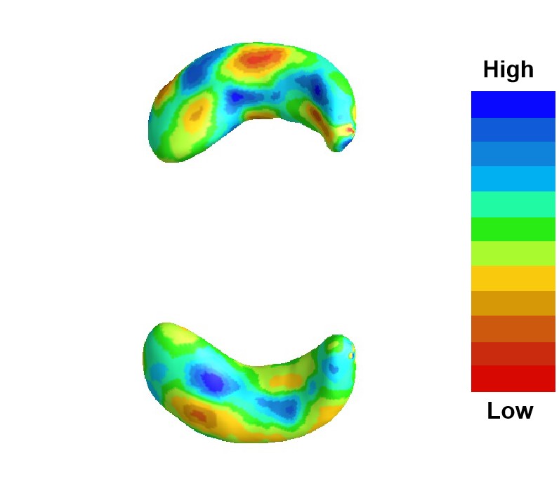
Figure 1: The Hippocampus 3D Shape Surface with coefficients

4.2 The corpus callosum Data Analysis

We consider another real data, the corpus callosum (CC), which is the largest white matter structure in the brain. CC has been a structure of high interest in many neuroimaging studies of neuro-developmental pathology. It helps the hemispheres share information, but it also contributes to the spread of seizure impulses from one side of the brain to the other. Recent research Raz et al. (2010); Witelson (1989) has investigated the individual differences in CC and their possible implications regarding interhemispheric connectivity for several years.

We consider the CC contour data obtained from the ADNI study to test the dependence between a high-dimensional variable and a random variable. In the ADNI dataset, the segmentation of the T1-weighted MRI and the calculation of the intracranial volume were done by using $FreeSurfer$ package created by Dale, Fischl and Sereno (1999), whereas the midsagittal CC area was calculated by using CCseg package. The CC data set includes 409 subjects with 223 healthy controls and 186 AD patients at baseline of the ADNI database. Each subject has a CC planar contour $Y_{j}$ with 50 landmarks and five covariates. We treat the CC planar contour $Y_{j}$ as a manifold-valued response in the Kendall planar shape space and all covariates in the Euclidean space. The Riemannian shape distance was calculated by R package $shapes$ Dryden (2019).

It is of interest to detect the significant variable associated with CC contour data. We applied the MDD test for dependence between five categorical covariates, gender, handedness, marital status, retirement and diagnosis at the significance level $\alpha=0.05.$ We also applied DC test and HHG test for the CC data. The result is summarized in Table 7. It reveals that the shape of CC planar contour are highly dependent on gender, AD diagnosis. It may indicate that gender and AD diagnosis are significant variables, which agree with Witelson (1989); Pan et al. (2017). This result also demonstrated that the MMD test performs better to test the significance of variable gender than HHG test.

We plot the mean trajectories of healthy controls (HC) and Alzheimer’s disease (AD). The similar process is conducted on the Male and Female. Both of the results are shown in Figure 2. It can be observed that there is an obvious difference of the shape between the AD disease and healthy controls. Compared to healthy controls, the spleen of AD patients seems to be less thinner and the isthmus is more rounded. Moreover, the splenium can be observed that it is thinner in male groups than in female groups. This could be an intuitive evidence to agree with the correlation between gender and the AD disease.

Table 7: The p-values for correlating CC contour data and five categorical covariates after BH correction.

covariates	MDD	DC	HHG
Gender	0.015	0.018	0.222
Handedness	0.482	0.499	0.461
Marital Status	0.482	0.744	0.773
Retirement	0.482	0.482	0.461
Diagnosis	0.015	0.018	0.045

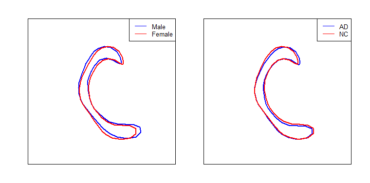
Figure 2: The corpus callosum Data Surface

5 Conclusion

In this paper, we propose the MDD statistics of correlation analysis for Non-Euclidean data in metric spaces and give some conditions for constructing the statistics. Then, we proved the mathematical preliminaries needed in our analysis. The proposed method is robust to outliers or heavy tails of the high dimensional variables. Depending on the results of simulations and real data analysis in hippocampus dataset from the ADNI, we demonstrate its usefulness for detecting correlations between the high dimensional variable and different types of variables (including genetic variables). We also demonstrate its usefulness in another manifold-valued data, CC contour data. We plan to explore our method to variable selection methods and other regression models.

Appendix: Technical details

Proof 5.1 (Proof of Theorem 1).

It is obvious that if $X$ and $Y$ are independent, $F_{r}(x,x^{\prime})=F(x,x^{\prime})$ for $\forall x,x^{\prime}\in\mathcal{M}$, then $MDD(X\mid Y)=0$. Next, we need to prove that if $MDD(X\mid Y)=0$, then $X$ and $Y$ are independent.

According to the definition of $MDD$, $MDD(X\mid Y)=\sum_{r=1}^{R}p_{r}\int[F_{r}(u,v)-F(u,v)]^{2}d\nu(u)d\nu(v)$. It is obvious that $MDD(X\mid Y)\geq 0$, so if $MDD(X\mid Y)=0$, we have $F_{r}(u,v)=F(u,v)$, $a.s.$ $\nu\otimes\nu$.

Given $Y=y_{r}$, define $\phi_{r}$ is a Borel probability measure of $X\mid Y=y_{r}$, and we have

$$\phi_{r}[\bar{B}(u,d(u,v))]:=F_{r}(u,v)=P(X\in\bar{B}(u,v)\mid Y=y_{r}).$$

Because $(\mathcal{M},d)$ is a Polish space that $d$ is directionally $(\epsilon,\eta,L)$-limited and we have $F_{r}(u,v)=F(u,v)$, $a.s.$ $\nu\otimes\nu$. Next, we can apply Theorem 1 in Wang et al. (2021) to get the conclusion that $\nu=\phi_{r}$ for $r=1,\ldots,R$.

Therefore, we have $F_{r}(x,x^{\prime})=F(x,x^{\prime})$ for $\forall x,x^{\prime}\in\mathbb{R}$. That is, for every $x$, $x^{\prime}$ and every $r$, we have

$$P(X\in\bar{B}(x,x^{\prime})\mid Y=y_{r})=P(X\in\bar{B}(x,x^{\prime})),$$

$i.e.$ $X$ and $Y$ are independent.

Proof 5.2 (Proof of Corollary 1).

(a) We have $\nu(\mathcal{U})\geq 1-\epsilon$ and the metric $d$ is directionally $(\epsilon,\eta,L)$-limited at $\mathcal{U}$, we can obtain the result of independence according to Theorem 1 and Corollary 1(a) in Wang et al. (2021).

(b) Similarly, we know that each $\mathcal{M}_{l}$ is a Polish space satisfying the directionally-limited condition, we also can obtain the result of independence according to Corollary 1(b) in Wang et al. (2021).

Proof 5.3 (Proof of Theorem 2).

Consider

$$\widehat{MDD}(X|Y)=\frac{1}{n^{2}}\sum_{r=1}^{R}\sum_{i=1}^{n}\sum_{j=1}^{n}\hat{p}_{r}[\hat{F}_{r}(X_{i},X_{j})-\hat{F}(X_{i},X_{j})]^{2}$$

$$= \frac{1}{n^{2}}\sum_{r=1}^{R}\sum_{i=1}^{n}\sum_{j=1}^{n}\hat{p}_{r}[\frac{1}{n}\sum_{k=1}^{n}\frac{I(X_{k}\in\bar{B}(X_{i},X_{j}),Y_{k}=y_{r})}{\hat{p}_{r}}$$

$$\quad\quad\quad\quad\quad\quad\quad-\frac{1}{n}\sum_{k=1}^{n}I(X_{k}\in\bar{B}(X_{i},X_{j})]^{2}$$

$$= \sum_{r=1}^{R}\Big{[}\frac{1}{n^{4}\hat{p}_{r}}\sum_{i,j,k,k^{\prime}=1}^{n}I(X_{k}\in\bar{B}(X_{i},X_{j}),Y_{k}=y_{r})$$

$$\quad\quad\quad\quad\quad\quad\quad\quad\quad I(X_{k^{\prime}}\in\bar{B}(X_{i},X_{j}),Y_{k^{\prime}}=y_{r})$$

$$+\frac{\hat{p}_{r}}{n^{4}}\sum_{i,j,k,k^{\prime}=1}^{n}I(X_{k}\in\bar{B}(X_{i},X_{j}))I(X_{k^{\prime}}\in\bar{B}(X_{i},X_{j}))$$

$$-\frac{1}{n^{4}}\sum_{i,j,k,k^{\prime}=1}[I(X_{k}\in\bar{B}(X_{i},X_{j}),Y_{k}=y_{r})I(X_{k^{\prime}}\in\bar{B}(X_{i},X_{j}))$$

$$-\frac{1}{n^{4}}\sum_{i,j,k,k^{\prime}=1}I(X_{k^{\prime}}\in\bar{B}(X_{i},X_{j}),Y_{k^{\prime}}=y_{r})I(X_{k}\in\bar{B}(X_{i},X_{j}))\Big{]}$$

$$= :Q_{1}+Q_{2}+Q_{3}.$$

For $Q_{1}$, $\frac{1}{n^{4}}\sum_{i,j,k,k^{\prime}=1}^{n}I(X_{k}\in\bar{B}(X_{i},X_{j}),Y_{k}=y_{r})I(X_{k^{\prime}}\in\bar{B}(X_{i},X_{j}),Y_{k^{\prime}}=y_{r})$ is a V-statistic of order 4. We can verify that

$$E[I(X_{k}\in\bar{B}(X_{i},X_{j}),Y_{k}=y_{r})I(X_{k^{\prime}}\in\bar{B}(X_{i},X_{j}),Y_{k^{\prime}}=y_{r})]$$

$$= E[E[I(X_{k}\in\bar{B}(X_{i},X_{j}),Y_{k}=y_{r})|X_{i},X_{j}]$$

$$\times E[I(X_{k^{\prime}}\in\bar{B}(X_{i},X_{j}),Y_{k^{\prime}}=y_{r})|X_{i},X_{j}]]$$

$$= E[E^{2}[I(X_{k}\in\bar{B}(X_{i},X_{j}),Y_{k}=y_{r})|X_{i},X_{j}]]$$

$$= p_{r}^{2}E[\frac{1}{p_{r}^{2}}E^{2}[I(X_{k}\in\bar{B}(X_{i},X_{j}),Y_{k}=y_{r})|X_{i},X_{j}]]$$

$$= p_{r}^{2}E[F_{r}^{2}(X_{i},X_{j})].$$

Since $E|I(X_{k}\in\bar{B}(X_{i},X_{j}),Y_{k}=y_{r})I(X_{k^{\prime}}\in\bar{B}(X_{i},X_{j}),Y_{k^{\prime}}=y_{r})|\leq 1<\infty$, according to Theorem 3 of Lee (2019), $\frac{1}{n^{4}}\sum_{i,j,k,k^{\prime}=1}^{n}I(X_{k}\in\bar{B}(X_{i},X_{j}),Y_{k}=y_{r})I(X_{k^{\prime}}\in\bar{B}(X_{i},X_{j}),Y_{k^{\prime}}=y_{r})$ almost surely converges to $p_{r}^{2}E[F_{r}^{2}(X_{i},X_{j})]$. And we have $p_{r}\to\hat{p}_{r}$, and we can draw conclusion that $Q_{1}\stackrel{{\scriptstyle a.s.}}{{\longrightarrow}}\sum_{r=1}^{R}p_{r}E[F_{r}^{2}(X_{i},X_{j})]$, as $n\to\infty$.

Similarly, we also have $Q_{2}\stackrel{{\scriptstyle a.s.}}{{\longrightarrow}}\sum_{r=1}^{R}p_{r}E[F^{2}(X_{i},X_{j})]$ and $Q_{3}\stackrel{{\scriptstyle a.s.}}{{\longrightarrow}}-2\sum_{r=1}^{R}p_{r}E[F_{r}(X_{i},X_{j})F(X_{i},X_{j})]$, as $n\to\infty$.

Because $MDD(X|Y)=E[\sum_{r=1}^{R}p_{r}(F_{r}(X_{i},X_{j})-F(X_{i},X_{j}))^{2}]$, we have

$$\widehat{MDD}(X|Y)\stackrel{{\scriptstyle a.s.}}{{\longrightarrow}}MDD(X|Y),~{}n\to\infty.$$

Before we prove Theorem 3, we give an lemma and some notations as follows Lee (2019).

Lemma 5.4.

Let $V_{n}$ be a V-statistic of order m, where $V_{n}=n^{-m}\sum_{i_{1}=1}^{n}\cdots\sum_{i_{m}=1}^{n}h(X_{i_{1}},\ldots,X_{i_{m}})$ and $h(X_{i_{1}},\ldots,X_{i_{m}})$ is the kernel of $V_{n}$. For all $1\leq i_{1}\leq\cdots\leq i_{m}\leq m$, $E[h(X_{i_{1}},\ldots,X_{i_{m}})]^{2}<\infty$. We have the following conclusions.

(i) If $\zeta_{1}=\mathrm{Var}(h_{1}(X_{1}))>0$, then

$$\sqrt{n}(V_{n}-E(h(X_{1},\ldots,X_{m})))\stackrel{{\scriptstyle d}}{{\rightarrow}}N(0,m^{2}\zeta_{1}),$$

where $\zeta_{k}=\mathrm{Var}(h_{k}(X_{1},\ldots,X_{K}))$ and

$$h_{k}(X_{1},\ldots,X_{K})= E[h(X_{1},\ldots,X_{m})|X_{1}=x_{1},\ldots,X_{k}=x_{k}]$$

$$= E[h(x_{1},\ldots,x_{k},X_{k+1},\ldots,X_{m})].$$

(ii) If $\zeta_{1}=0$ but $\zeta_{2}=\mathrm{Var}(h_{2}(X_{1},X_{2}))>0$, then $n(V_{n}-E(h(X_{1},\ldots,X_{m})))\stackrel{{\scriptstyle d}}{{\rightarrow}}\frac{m(m-1)}{2}\sum_{j=1}^{\infty}\lambda_{j}\mathcal{X}_{j}^{2}(1)$, where $\mathcal{X}_{j}^{2}(1)$’s, $j=1,2,\ldots$, are independently and identically distributed $\mathcal{X}^{2}$ random variables with $1$ degree of freedom and $\lambda_{j}$’s meet the condition $\sum_{j=1}^{\infty}\lambda_{j}^{2}=\zeta_{2}$.

Proof 5.5 (Proof of Theorem 3).

Denote $Z_{i}=(X_{i},Y_{i})$, $Z_{j}=(X_{j},Y_{j})$, $Z_{k}=(X_{k},Y_{k})$, $Z_{k^{\prime}}=(X_{k^{\prime}}$, $Y_{k^{\prime}})$. We consider the statistic with the known parameter $p_{r}$

$$I_{n}= \frac{1}{n^{2}}\sum_{r=1}^{R}\sum_{i=1}^{n}\sum_{j=1}^{n}p_{r}[\frac{1}{n}\sum_{k=1}^{n}\frac{I(X_{k}\in\bar{B}(X_{i},X_{j}),Y_{k}=y_{r})}{p_{r}}$$

$$\quad\quad\quad\quad\quad\quad\quad-\frac{1}{n}\sum_{k=1}^{n}I(X_{k}\in\bar{B}(X_{i},X_{j})]^{2}$$

$$= \frac{1}{n^{4}}\sum_{r=1}^{R}\sum_{i=1}^{n}\sum_{j=1}^{n}\sum_{k,k^{\prime}=1}^{n}[\frac{1}{p_{r}}I(X_{k}\in\bar{B}(X_{i},X_{j}),Y_{k}=y_{r})$$

$$\quad\quad\quad\quad\quad\quad\quad\quad\quad\times I(X_{k^{\prime}}\in\bar{B}(X_{i},X_{j}),Y_{k^{\prime}}=y_{r})$$

$$+p_{r}I(X_{k}\in\bar{B}(X_{i},X_{j}))I(X_{k^{\prime}}\in\bar{B}(X_{i},X_{j}))$$

$$-I(X_{k}\in\bar{B}(X_{i},X_{j}),Y_{k}=y_{r})I(X_{k^{\prime}}\in\bar{B}(X_{i},X_{j}))$$

$$-I(X_{k^{\prime}}\in\bar{B}(X_{i},X_{j}),Y_{k^{\prime}}=y_{r})I(X_{k}\in\bar{B}(X_{i},X_{j}))].$$

Let $V_{n}^{p_{r}}=\frac{1}{n^{4}}\sum_{i,j,k,k^{\prime}=1}^{n}\Psi^{(r)}(Z_{i},Z_{j},Z_{k},Z_{k^{\prime}})$ and

$$\Psi^{(r)}(Z_{i},Z_{j},Z_{k},Z_{k^{\prime}})$$

$$= \frac{1}{p_{r}}I(X_{k}\in\bar{B}(X_{i},X_{j}),Y_{k}=y_{r})I(X_{k^{\prime}}\in\bar{B}(X_{i},X_{j}),Y_{k^{\prime}}=y_{r})$$

$$+p_{r}I(X_{k}\in\bar{B}(X_{i},X_{j}))I(X_{k^{\prime}}\in\bar{B}(X_{i},X_{j}))$$

$$-I(X_{k}\in\bar{B}(X_{i},X_{j}),Y_{k}=y_{r})I(X_{k^{\prime}}\in\bar{B}(X_{i},X_{j}))$$

$$-I(X_{k^{\prime}}\in\bar{B}(X_{i},X_{j}),Y_{k^{\prime}}=y_{r})I(X_{k}\in\bar{B}(X_{i},X_{j})),$$

then we have

$$I_{n}= \sum_{r=1}^{R}V_{n}^{(p_{r})}$$

$$= \sum_{r=1}^{R}\frac{1}{n^{4}}\sum_{i,j,k,k^{\prime}=1}^{n}\Psi^{(r)}(Z_{i},Z_{j},Z_{k},Z_{k^{\prime}}).$$

We would like to use V statistic to obatain the asymptotic properties of $\widehat{MDD}(X|Y)$. We symmetrize the kernel $\Psi^{(r)}(Z_{i},Z_{j},Z_{k},Z_{k^{\prime}})$ and denote

$$\Psi^{(r)}_{S}(Z_{i},Z_{j},Z_{k},Z_{k^{\prime}})$$

$$= \frac{1}{4!}\sum_{\tau\in\pi(i,j,k,k^{\prime})}\Psi^{(r)}(Z_{\tau(1)},Z_{\tau(2)},Z_{\tau(3)},Z_{\tau(4)}),$$

where $\pi(i,j,k,k^{\prime})$ are the permutations of $\{i,j,k,k^{\prime}\}$. Now, the kernel $\Psi^{(r)}_{S}(Z_{i},Z_{j},Z_{k},Z_{k^{\prime}})$ is symmetric, and $\frac{1}{n^{4}}\sum_{i,j,k,k^{\prime}=1}^{n}\Psi^{(r)}_{S}(Z_{i},Z_{j},Z_{k},Z_{k^{\prime}})$ should be a V-statistic. By using the denotation of Lemma 5.4, we should consider $E[\Psi^{(r)}_{S}(z_{i},Z_{j},Z_{k},Z_{k^{\prime}})]$, that is, the case where only one random variable fixed its value. And, we have to consider $E[\Psi^{(r)}(z_{i},Z_{j},Z_{k},Z_{k^{\prime}})]$, $E[\Psi^{(r)}(Z_{i},z_{j},Z_{k},Z_{k^{\prime}})]$, $E[\Psi^{(r)}(Z_{i},Z_{j},z_{k},Z_{k^{\prime}})]$ and $E[\Psi^{(r)}(Z_{i},Z_{j},Z_{k},z_{k^{\prime}})]$.

We consider

$$E[\Psi^{(r)}(z_{i},Z_{j},Z_{k},Z_{k^{\prime}})]$$

$$= \frac{1}{p_{r}}E[I(X_{k}\in\bar{B}(x_{i},X_{j}),Y_{k}=y_{r})$$

$$\quad\quad I(X_{k^{\prime}}\in\bar{B}(x_{i},X_{j}),Y_{k^{\prime}}=y_{r})]$$

$$+p_{r}E[I(X_{k}\in\bar{B}(x_{i},X_{j}))I(X_{k^{\prime}}\in\bar{B}(x_{i},X_{j}))]$$

$$-E[I(X_{k}\in\bar{B}(x_{i},X_{j}),Y_{k}=y_{r})I(X_{k^{\prime}}\in\bar{B}(x_{i},X_{j}))]$$

$$-E[I(X_{k^{\prime}}\in\bar{B}(x_{i},X_{j}),Y_{k^{\prime}}=y_{r})I(X_{k}\in\bar{B}(x_{i},X_{j}))]$$

$$= \frac{1}{p_{r}}P_{j,k,k^{\prime}}[X_{k},X_{k^{\prime}}\in\bar{B}(x_{i},X_{j}),Y_{k}=Y_{k^{\prime}}=y_{r})]$$

$$+p_{r}P_{j,k,k^{\prime}}[X_{k},X_{k^{\prime}}\in\bar{B}(x_{i},X_{j})]$$

$$-P_{j,k,k^{\prime}}[X_{k},X_{k^{\prime}}\in\bar{B}(x_{i},X_{j}),Y_{k}=y_{r}]$$

$$-P_{j,k,k^{\prime}}[X_{k},X_{k^{\prime}}\in\bar{B}(x_{i},X_{j}),Y_{k^{\prime}}=y_{r}],$$

where $P_{j,k,k^{\prime}}$ means the probability of $Z_{j}$, $Z_{k}$ and $Z_{k^{\prime}}$.

Under the null hypothesis $H_{0}$, $X$ and $Y$ are independent. Then we have

$$\frac{1}{p_{r}}P_{j,k,k^{\prime}}[X_{k},X_{k^{\prime}}\in\bar{B}(x_{i},X_{j}),Y_{k}=Y_{k^{\prime}}=y_{r}]$$

$$= \frac{1}{p_{r}}P_{j,k,k^{\prime}}[X_{k},X_{k^{\prime}}\in\bar{B}(x_{i},X_{j}),Y_{k}=y_{r}]P_{k^{\prime}}[Y_{k^{\prime}}=y_{r}]$$

$$= P_{j,k,k^{\prime}}[X_{k},X_{k^{\prime}}\in\bar{B}(x_{i},X_{j}),Y_{k}=y_{r}],$$

and

$$p_{r}P_{j,k,k^{\prime}}[X_{k},X_{k^{\prime}}\in\bar{B}(x_{i},X_{j})]$$

$$= P_{j,k,k^{\prime}}[X_{k},X_{k^{\prime}}\in\bar{B}(x_{i},X_{j}),Y_{k^{\prime}}=y_{r}],$$

Thus, $E[\Psi^{(r)}(z_{i},Z_{j},Z_{k},Z_{k^{\prime}})]=0$.

Similarly, we have $E[\Psi^{(r)}(Z_{i},z_{j},Z_{k},Z_{k^{\prime}})]=0$, $E[\Psi^{(r)}(Z_{i},Z_{j},z_{k},Z_{k^{\prime}})]=0$ and $E[\Psi^{(r)}(Z_{i},Z_{j},Z_{k},z_{k^{\prime}})]=0$ because of the independence of $X$ and $Y$ under the null hypothesis $H_{0}$.

Next, we consider the case when two random elements are fixed.

$$E[\Psi^{(r)}(Z_{i},Z_{j},z_{k},z_{k^{\prime}})]$$

$$= \frac{1}{p_{r}}E[I(x_{k}\in\bar{B}(X_{i},X_{j}),y_{k}=y_{r})$$

$$\quad\quad\times I(x_{k^{\prime}}\in\bar{B}(X_{i},X_{j}),y_{k^{\prime}}=y_{r})]$$

$$+p_{r}E[I(x_{k}\in\bar{B}(X_{i},X_{j}))I(x_{k^{\prime}}\in\bar{B}(X_{i},X_{j}))]$$

$$-E[I(x_{k}\in\bar{B}(X_{i},X_{j}),y_{k}=y_{r})I(x_{k^{\prime}}\in\bar{B}(X_{i},X_{j}))]$$

$$-E[I(x_{k^{\prime}}\in\bar{B}(X_{i},X_{j}),y_{k^{\prime}}=y_{r})I(x_{k}\in\bar{B}(X_{i},X_{j}))]$$

$$= \frac{1}{p_{r}}P_{i,j}[x_{k},x_{k^{\prime}}\in\bar{B}(X_{i},X_{j}),y_{k}=y_{k^{\prime}}=y_{r})]$$

$$+p_{r}P_{i,j}[x_{k},x_{k^{\prime}}\in\bar{B}(X_{i},X_{j})]$$

$$-P_{i,j}[x_{k},x_{k^{\prime}}\in\bar{B}(X_{i},X_{j}),y_{k}=y_{r}]$$

$$-P_{i,j}[x_{k},x_{k^{\prime}}\in\bar{B}(X_{i},X_{j}),y_{k^{\prime}}=y_{r}],$$

$E[\Psi^{(r)}(Z_{i},Z_{j},z_{k},z_{k^{\prime}})]$ is a non-constant function related to $z_{k},z_{k^{\prime}}$.

In addition, we know

$$E[\Psi^{(r)}(Z_{i},Z_{j},Z_{k},Z_{k^{\prime}})]$$

$$= \frac{1}{p_{r}}E[I(X_{k}\in\bar{B}(X_{i},X_{j}),Y_{k}=y_{r})$$

$$\quad\quad\times I(X_{k^{\prime}}\in\bar{B}(X_{i},X_{j}),Y_{k^{\prime}}=y_{r})]$$

$$+p_{r}E[I(X_{k}\in\bar{B}(X_{i},X_{j}))I(X_{k^{\prime}}\in\bar{B}(X_{i},X_{j}))]$$

$$-E[I(X_{k}\in\bar{B}(X_{i},X_{j}),Y_{k}=y_{r})I(X_{k^{\prime}}\in\bar{B}(X_{i},X_{j}))]$$

$$-E[I(X_{k^{\prime}}\in\bar{B}(X_{i},X_{j}),Y_{k^{\prime}}=y_{r})I(X_{k}\in\bar{B}(X_{i},X_{j}))]$$

$$= \frac{1}{p_{r}}P_{i,j,k,k^{\prime}}[X_{k},X_{k^{\prime}}\in\bar{B}(X_{i},X_{j}),Y_{k}=Y_{k^{\prime}}=y_{r})]$$

$$+p_{r}P_{i,j,k,k^{\prime}}[X_{k},X_{k^{\prime}}\in\bar{B}(X_{i},X_{j})]$$

$$-P_{i,j,k,k^{\prime}}[X_{k},X_{k^{\prime}}\in\bar{B}(X_{i},X_{j}),Y_{k}=y_{r}]$$

$$-P_{i,j,k,k^{\prime}}[X_{k},X_{k^{\prime}}\in\bar{B}(X_{i},X_{j}),Y_{k^{\prime}}=y_{r}]=0,$$

The last equation is derived from the independence of $X$ and $Y$. By Lemma 5.4 $(ii)$, $V_{n}^{(p_{r})}$ is a limiting $\chi^{2}$-type V statistic.

Now, we consider $V_{n}^{(\hat{p}_{r})}$. Let $t=(t_{1},t_{2})$. In showing the conditions of Theorem 2.16 in de Wet and Randles (1987) hold, we use

$$h(z_{1},z_{2};p_{r})=p_{r}\int g(z_{1},t;p_{r})g(z_{2},t;p_{r})dM(t),$$

where $g(z,t;\gamma)=\sqrt{p_{r}}(I(z\in\bar{B}(t_{1},t_{2}),y_{1}=y_{r})/\gamma-I(z\in\bar{B}(t_{1},t_{2})))$ and $=\nu\otimes\nu$ is the product measure of $\nu$ with respect to $X$.

Thus,

$$\mu(t;\gamma)= Eg(Z,t;\gamma)$$

$$= \sqrt{\gamma}(P(X\in\bar{B}(t_{1},t_{2}))p_{r}/\gamma-P(X\in\bar{B}(t_{1},t_{2})))$$

and

$$\mathbf{d}_{1}\mu(t;p_{r})=p_{r}^{-\frac{1}{2}}P(X\in\bar{B}(t_{1},t_{2})).$$

The condition of Theorem 2.16 in de Wet and Randles (1987) can be shown to hold in this case using

$$h_{*} (Z_{1},Z_{2})$$

$$=\int [g(Z_{1},t;p_{r})+\mathbf{d}_{1}\mu(t;p_{r})(I(Y_{1}=y_{r})-p_{r})]$$

$$[g(Z_{2},t;p_{r})+\mathbf{d}_{1}\mu(t;p_{r})(I(Y_{2}=y_{r})-p_{r})]dM(t).$$

Let $\{\lambda_{i}\}$ denote the eigenvalues of the operator $A$ defined by

$$Aq(x)=\int h_{*}(z_{1},z_{2})q(y)d\nu(x_{2})dP(y_{2}),$$

then

$$nV_{n}^{(\hat{p}_{r})}\stackrel{{\scriptstyle d}}{{\rightarrow}}\sum_{j=1}^{\infty}\lambda_{j}^{(r)}\mathcal{X}_{j}^{2}(1),$$

where $\mathcal{X}_{j}^{2}(1)^{\prime}s$, $j=1,2,\ldots$, are independently and identically distributed chi-square distribution with 1 degree of freedom.

Notice that $\widehat{MDD}(X|Y)=\sum_{r=1}^{R}V_{n}^{(r)}$, according to the independence of the sample and the additivity of chi-square distribution,

$$n\widehat{MDD}(X|Y)\stackrel{{\scriptstyle d}}{{\rightarrow}}\sum_{j=1}^{\infty}\lambda_{j}\mathcal{X}_{j}^{2}(1),$$

where $\lambda_{j}=\sum_{r=1}^{R}\lambda_{j}^{(r)}$.

Proof 5.6 (Proof of Theorem 4).

Under the alternative hypothesis $H_{1}$, $\widehat{MDD}(X|Y)\stackrel{{\scriptstyle a.s.}}{{\longrightarrow}}MDD(X|Y)>0$, as $n\rightarrow\infty$. Thus, we have $n\widehat{MDD}(X|Y)\stackrel{{\scriptstyle a.s.}}{{\longrightarrow}}\infty$, as $n\rightarrow\infty$.

Proof 5.7 (Proof of Theorem 5).

We consider

$$\widehat{MDD}(X|Y)=I_{n}+J_{n},$$

where

$$I_{n}= \sum_{r=1}^{R}\frac{1}{n^{4}}\sum_{i,j,k,k^{\prime}=1}^{n}\frac{1}{p_{r}}I(X_{k}\in\bar{B}(X_{i},X_{j}),Y_{k}=y_{r})$$

$$\quad\quad\quad\quad\quad\quad\quad\times I(X_{k^{\prime}}\in\bar{B}(X_{i},X_{j}),Y_{k^{\prime}}=y_{r})$$

$$+ \sum_{r=1}^{R}\frac{1}{n^{4}}\sum_{i,j,k,k^{\prime}=1}^{n}p_{r}I(X_{k}\in\bar{B}(X_{i},X_{j}))I(X_{k^{\prime}}\in\bar{B}(X_{i},X_{j}))$$

$$- \sum_{r=1}^{R}\frac{1}{n^{4}}\sum_{i,j,k,k^{\prime}=1}^{n}I(X_{k}\in\bar{B}(X_{i},X_{j}),Y_{k}=y_{r})$$

$$\quad\quad\quad\quad\quad\quad\quad\times I(X_{k^{\prime}}\in\bar{B}(X_{i},X_{j}))$$

$$- \sum_{r=1}^{R}\frac{1}{n^{4}}\sum_{i,j,k,k^{\prime}=1}^{n}I(X_{k^{\prime}}\in\bar{B}(X_{i},X_{j}),Y_{k^{\prime}}=y_{r})$$

$$\quad\quad\quad\quad\quad\quad\quad\times I(X_{k}\in\bar{B}(X_{i},X_{j}))$$

and

$$J_{n}= \sum_{r=1}^{R}(\frac{1}{\hat{p}_{r}}-\frac{1}{p_{r}})\frac{1}{n^{4}}\sum_{i,j,k,k^{\prime}=1}^{n}I(X_{k}\in\bar{B}(X_{i},X_{j}),Y_{k}=y_{r})$$

$$\quad\quad\quad\quad\quad\quad\quad\times I(X_{k^{\prime}}\in\bar{B}(X_{i},X_{j}),Y_{k^{\prime}}=y_{r})$$

$$+ \sum_{r=1}^{R}(\hat{p}_{r}-p_{r})\frac{1}{n^{4}}\sum_{i,j,k,k^{\prime}=1}^{n}I(X_{k}\in\bar{B}(X_{i},X_{j}))$$

$$\quad\quad\quad\quad\quad\quad\quad\times I(X_{k^{\prime}}\in\bar{B}(X_{i},X_{j})).$$

We consider $E[\Psi^{(r)}(z_{i},Z_{j},Z_{k},Z_{k^{\prime}})]$ in the proof of Theorem 3,

$$E[\Psi^{(r)}(z_{i},Z_{j},Z_{k},Z_{k^{\prime}})]$$

$$= \frac{1}{p_{r}}P_{j,k,k^{\prime}}[X_{k},X_{k^{\prime}}\in\bar{B}(x_{i},X_{j}),Y_{k}=Y_{k^{\prime}}=y_{r})]$$

$$+p_{r}P_{j,k,k^{\prime}}[X_{k},X_{k^{\prime}}\in\bar{B}(x_{i},X_{j})]$$

$$-P_{j,k,k^{\prime}}[X_{k},X_{k^{\prime}}\in\bar{B}(x_{i},X_{j}),Y_{k}=y_{r}]$$

$$-P_{j,k,k^{\prime}}[X_{k},X_{k^{\prime}}\in\bar{B}(x_{i},X_{j}),Y_{k^{\prime}}=y_{r}].$$

Under the alternative hypothesis $H_{1}$, $X$ and $Y$ is not independent of each other, i.e.

$$\frac{1}{p_{r}}P_{j,k,k^{\prime}}[X_{k},X_{k^{\prime}}\in\bar{B}(x_{i},X_{j}),Y_{k}=Y_{k^{\prime}}=y_{r}]$$

$$\neq P_{j,k,k^{\prime}}[X_{k},X_{k^{\prime}}\in\bar{B}(x_{i},X_{j}),Y_{k}=y_{r}],$$

and

$$p_{r}P_{j,k,k^{\prime}}[X_{k},X_{k^{\prime}}\in\bar{B}(x_{i},X_{j})]$$

$$\neq P_{j,k,k^{\prime}}[X_{k},X_{k^{\prime}}\in\bar{B}(x_{i},X_{j}),Y_{k^{\prime}}=y_{r}],$$

so $E[\Psi^{(r)}(z_{i},Z_{j},Z_{k},Z_{k^{\prime}})]$ is a non-constant function related to $z_{i}$, and we know $h_{1}^{(r)}(Z_{1})=\frac{1}{4}[E[\Psi^{(r)}(z_{i},Z_{j},Z_{k},Z_{k^{\prime}})]+E[\Psi^{(r)}(Z_{i},z_{j},Z_{k},Z_{k^{\prime}})]+E[\Psi^{(r)}(Z_{i},Z_{j},z_{k},Z_{k^{\prime}})]+E[\Psi^{(r)}(Z_{i},Z_{j},Z_{k},z_{k^{\prime}})]]$, then we have $\mathrm{Var}[h_{1}^{(r)}(Z_{1})]>0$. We apply Lemma 5.4 $(i)$, we have

$$\sqrt{n}[V_{n}^{(p_{r})}-E[\Psi^{(r)}(Z_{i},Z_{j},Z_{k},Z_{k^{\prime}})]]\stackrel{{\scriptstyle d}}{{\rightarrow}}N(0,16\mathrm{Var}[h_{1}^{(r)}(Z_{1})]),$$

Because $I_{n}=\sum_{r=1}^{R}V_{n}^{(p_{r})}$, $MDD(X|Y)=E[\sum_{r=1}^{R}p_{r}(F_{r}(X_{i},X_{j})-F(X_{i},X_{j}))^{2}]$ and

$$E[\Psi^{(r)}(Z_{i},Z_{j},Z_{k},Z_{k^{\prime}})]$$

$$= E[E[\Psi^{(r)}(Z_{i},Z_{j},Z_{k},Z_{k^{\prime}})|Z_{i},Z_{j}]]$$

$$= \frac{1}{p_{r}}E[E[I(X_{k}\in\bar{B}(X_{i},X_{j}),Y_{k}=y_{r})|Z_{i},Z_{j}]$$

$$\quad\quad E[I(X_{k^{\prime}}\in\bar{B}(X_{i},X_{j}),Y_{k^{\prime}}=y_{r})|Z_{i},Z_{j}]]$$

$$+p_{r}E[E[I(X_{k}\in\bar{B}(X_{i},X_{j}))|Z_{i},Z_{j}]$$

$$\quad\quad E[I(X_{k^{\prime}}\in\bar{B}(X_{i},X_{j}))|Z_{i},Z_{j}]]$$

$$-E[E[I(X_{k}\in\bar{B}(X_{i},X_{j}),Y_{k}=y_{r})|Z_{i},Z_{j}]$$

$$\quad\quad\quad E[I(X_{k^{\prime}}\in\bar{B}(X_{i},X_{j}))|Z_{i},Z_{j}]]$$

$$-E[E[I(X_{k^{\prime}}\in\bar{B}(X_{i},X_{j}),Y_{k^{\prime}}=y_{r})|Z_{i},Z_{j}]$$

$$\quad\quad E[I(X_{k}\in\bar{B}(X_{i},X_{j}))|Z_{i},Z_{j}]]$$

$$= \frac{1}{p_{r}}E[E^{2}[I(X_{k}\in\bar{B}(X_{i},X_{j}),Y_{k}=y_{r})|Z_{i},Z_{j}]]$$

$$+p_{r}E[E^{2}[I(X_{k}\in\bar{B}(X_{i},X_{j}))|Z_{i},Z_{j}]]$$

$$-2E[E[I(X_{k}\in\bar{B}(X_{i},X_{j}),Y_{k}=y_{r})|Z_{i},Z_{j}]$$

$$\quad\quad\quad E[I(X_{k}\in\bar{B}(X_{i},X_{j}))|Z_{i},Z_{j}]]$$

$$= p_{r}E[(\frac{1}{p_{r}}E[I(X_{k}\in\bar{B}(X_{i},X_{j}),Y_{k}=y_{r})|Z_{i},Z_{j}]$$

$$-E[I(X_{k}\in\bar{B}(X_{i},X_{j}))|Z_{i},Z_{j}])^{2}]$$

$$= E[p_{r}(F_{r}(X_{i},X_{j})-F(X_{i},X_{j}))^{2}],$$

we have

$$E[\Psi^{(r)}(Z_{i},Z_{j},Z_{k},Z_{k^{\prime}})]]=\sum_{r=1}^{R}MDD(X|Y)$$

and

$$\sqrt{n}[I_{n}-MDD(X|Y)]\stackrel{{\scriptstyle d}}{{\rightarrow}}N(0,\sigma_{I}^{2}),$$

where $\sigma_{I}^{2}=\sum_{r=1}^{R}16\mathrm{Var}[h_{1}^{(r)}(Z_{i})]+2n\sum_{i<j}Cov(V_{n}^{(i)},V_{n}^{(j)})$. We explain here that $Cov(V_{n}^{(i)},V_{n}^{(j)})$ is the covariance of V-statistic $V_{n}^{(i)}$ and $V_{n}^{(j)}$ of order 4, which can be written as $Cov(V_{n}^{(i)},V_{n}^{(j)})=\frac{1}{n^{4}}\sum_{c=1}^{4}\binom{4}{c}(n-4)^{4-c}\sigma_{c,c}^{2}$, where $\sigma_{c,c}^{2}=Cov(h_{c}^{(p)}(Z_{1},\ldots,Z_{c}),h_{c}^{(q)}(Z_{1},\ldots,Z_{c}))$ and $h_{c}^{(p)}(Z_{1},\ldots,Z_{c})$ represents $h_{c}(Z_{1},\ldots,Z_{c})$ of Lemma 5.4 when $r=p$.

Next, we would like to know the asymptotic distribution of $\sqrt{n}[\widehat{MDD}(X|Y)-MDD(X|Y)]$, we need to consider the asymptotic distribution of $\sqrt{n}J_{n}$ as follows

$$\sqrt{n}[\widehat{MDD}(X|Y)-MDD(X|Y)]$$

$$= \sqrt{n}[I_{n}+J_{n}-MDD(X|Y)].$$

Then, we consider $J_{n}$. Denote $V_{1}^{(r)}=\frac{1}{n^{4}}\sum_{i,j,k,k^{\prime}=1}^{n}I(X_{k}\in\bar{B}(X_{i},X_{j}),Y_{k}=y_{r})I(X_{k^{\prime}}\in\bar{B}(X_{i},X_{j}),Y_{k^{\prime}}=y_{r})$ and $V_{2}=\frac{1}{n^{4}}\sum_{i,j,k,{k^{\prime}}=1}^{n}I(X_{k}\in\bar{B}(X_{i},X_{j}))I(X_{k^{\prime}}\in\bar{B}(X_{i},X_{j}))$, we have

$$J_{n}=\sum_{r=1}^{R}(\hat{p}_{r}-p_{r})(V_{2}-\frac{1}{\hat{p}_{r}p_{r}}V_{1}^{(r)}).$$

The asymptotic distribution of $V_{2}-\frac{1}{\hat{p}_{r}p_{r}}V_{1}^{(r)}$ is a constant, because we know $E[V_{1}^{(r)}]=E[I(X_{k}\in\bar{B}(X_{i},X_{j}),Y_{k}=y_{r})I(X_{k^{\prime}}\in\bar{B}(X_{i},X_{j}),Y_{k^{\prime}}=y_{r})]=p_{r}^{2}E[F_{r}^{2}(X_{i},X_{j})]$, $E[V_{2}]=E[I(X_{k}\in\bar{B}(X_{i},X_{j})I(X_{k^{\prime}}\in\bar{B}(X_{i},X_{j})]=E[F^{2}(X_{i},X_{j})]$ and $\hat{p}_{r}\rightarrow p_{r}$. Then

$$V_{2}-\frac{1}{\hat{p}_{r}p_{r}}V_{1}^{(r)}\rightarrow E[F^{2}(X_{i},X_{j})]-E[F_{r}^{2}(X_{i},X_{j})].$$

According to the Central Limit Theorem (CLT), for arbitrary $r=1,\ldots,R$, we have

$$\sqrt{n}(\hat{p}_{r}-p_{r})(V_{2}-\frac{1}{\hat{p}_{r}p_{r}}V_{1}^{(r)})\rightarrow N(0,\sigma_{r}^{2}),$$

where $\sigma_{r}^{2}=p_{r}(1-p_{r})(E[F^{2}(X_{i},X_{j})]-E[F_{r}^{2}(X_{i},X_{j})])$.

Let $\mathbf{\hat{p}}^{(i)}=(I(Y_{i}=y_{1}),I(Y_{i}=y_{2}),\ldots,I(Y_{i}=y_{R}))^{T}$, where $\mathbf{\hat{p}}^{(i)}$ is a $R$-dimensional random variable and $\mathbf{\hat{p}}^{(1)},\mathbf{\hat{p}}^{(2)},\ldots,\mathbf{\hat{p}}^{(n)}$ is dependent of each other. Therefore, according to multidimensional CLT, $\sqrt{n}(\frac{1}{n}\sum_{i=1}^{n}\mathbf{\hat{p}}^{(i)}-E[\mathbf{\hat{p}}^{(i)}])=(\sqrt{n}(\hat{p}_{1}-p_{1}),\ldots,\sqrt{n}(\hat{p}_{R}-p_{R}))^{T}$ asymptotically obey the $R$-dimensional normal distribution. In this way we get the condition of the additivity of the normal distribution, then we have

$$\sqrt{n}J_{n}\rightarrow N(0,\sigma_{J}^{2}),$$

where $\sigma_{J}^{2}=\sum_{r=1}^{R}\sigma_{r}^{2}+2\sum_{i<j}Cov(\hat{p}_{i},\hat{p}_{j})=\sum_{r=1}^{R}\sigma_{r}^{2}-\frac{2}{n}\sum_{i<j}p_{i}p_{j}=\sum_{r=1}^{R}p_{r}(1-p_{r})(E[F^{2}(X_{i},X_{j})]-E[F_{r}^{2}(X_{i},X_{j})])-\frac{2}{n}\sum_{i<j}p_{i}p_{j}$.

Similarly, we can use multidimensional CLT to prove $\sqrt{n}J_{n}$ and $\sqrt{n}[I_{n}-MV(X|Y)]$ are bivariate normal distribution. Then, we make a conclusion,

$$\sqrt{n}[\widehat{MDD}(X|Y)-MDD(X|Y)]\stackrel{{\scriptstyle d}}{{\rightarrow}}N(0,\sigma^{2}),$$

where $\sigma^{2}=\sigma_{I}^{2}+\sigma_{J}^{2}+2nCov(I_{n},J_{n})\sigma_{I}\sigma_{J}$. We explain here that $Cov(I_{n},J_{n})$ is the covariance of V-statistic $I_{n}$ of order 4 and $J_{n}$ of order 1, which can be written as $Cov(I_{n},J_{n})=Cov(\sum_{r=1}^{R}V_{n}^{(r)},\sum_{r=1}^{R}(\hat{p}_{r}-p_{r})(V_{2}-\frac{1}{\hat{p}_{r}p_{r}}V_{1}^{(r)}))=\sum_{r=1}^{R}\sum_{r^{\prime}=1}^{R}Cov(V_{n}^{(r)},(\hat{p}_{r^{\prime}}-p_{r^{\prime}})(V_{2}-\frac{1}{\hat{p}_{r^{\prime}}p_{r^{\prime}}}V_{1}^{(r)}))=\sum_{r=1}^{R}\sum_{r^{\prime}=1}^{R}\frac{1}{n}\binom{4}{1}(n-4)^{3}Cov(h_{1}^{(r)}(Z_{1}),I(Y_{k}=y_{r^{\prime}}))(E[F^{2}(X_{i},X_{j})]-E[F_{r}^{2}(X_{i},X_{j})])$.

References

• Anand and Dhikav (2012) {barticle}[author] \bauthor\bsnmAnand, \bfnmKuljeet\binitsK. and \bauthor\bsnmDhikav, \bfnmVikas\binitsV. (\byear2012). \btitleHippocampus in health and disease: An overview. \bjournalAnnals of Indian Academy of Neurology \bvolume15 \bpages239-46. \bdoi10.4103/0972-2327.104323 \endbibitem
• Balasundaram, Butenko and Hicks (2011) {barticle}[author] \bauthor\bsnmBalasundaram, \bfnmBalabhaskar\binitsB., \bauthor\bsnmButenko, \bfnmSergiy\binitsS. and \bauthor\bsnmHicks, \bfnmIllya V\binitsI. V. (\byear2011). \btitleClique Relaxations in Social Network Analysis: The Maximum k-Plex Problem. \bjournalOperations Research \bvolume59 \bpages133–142. \endbibitem
• Benesty et al. (2009) {bincollection}[author] \bauthor\bsnmBenesty, \bfnmJacob\binitsJ., \bauthor\bsnmChen, \bfnmJingdong\binitsJ., \bauthor\bsnmHuang, \bfnmYiteng\binitsY. and \bauthor\bsnmCohen, \bfnmIsrael\binitsI. (\byear2009). \btitlePearson correlation coefficient. In \bbooktitleNoise reduction in speech processing \bpages1–4. \bpublisherSpringer. \endbibitem
• Bookstein (1996) {barticle}[author] \bauthor\bsnmBookstein, \bfnmFred L\binitsF. L. (\byear1996). \btitleBiometrics, biomathematics and the morphometric synthesis. \bjournalBulletin of Mathematical Biology \bvolume58 \bpages313–365. \endbibitem
• Charlier (2013) {barticle}[author] \bauthor\bsnmCharlier, \bfnmBenjamin\binitsB. (\byear2013). \btitleNecessary and sufficient condition for the existence of a Fréchet mean on the circle. \bjournalESAIM: Probability and Statistics \bvolume17 \bpages635–649. \endbibitem
• Şentürk and Müller (2010) {barticle}[author] \bauthor\bsnmŞentürk, \bfnmDamla\binitsD. and \bauthor\bsnmMüller, \bfnmHans-Georg\binitsH.-G. (\byear2010). \btitleFunctional varying coefficient models for longitudinal data. \bjournalJournal of the American Statistical Association \bvolume105 \bpages1256–1264. \endbibitem
• Şentürk and Nguyen (2011) {barticle}[author] \bauthor\bsnmŞentürk, \bfnmDamla\binitsD. and \bauthor\bsnmNguyen, \bfnmDanh V\binitsD. V. (\byear2011). \btitleVarying coefficient models for sparse noise-contaminated longitudinal data. \bjournalStatistica Sinica \bvolume21 \bpages1831. \endbibitem
• Cui and Zhong (2018) {barticle}[author] \bauthor\bsnmCui, \bfnmHengjian\binitsH. and \bauthor\bsnmZhong, \bfnmWei\binitsW. (\byear2018). \btitleA Distribution-Free Test of Independence and Its Application to Variable Selection. \bjournalarXiv: Methodology. \endbibitem
• Dale, Fischl and Sereno (1999) {barticle}[author] \bauthor\bsnmDale, \bfnmAnders M\binitsA. M., \bauthor\bsnmFischl, \bfnmBruce\binitsB. and \bauthor\bsnmSereno, \bfnmMartin I\binitsM. I. (\byear1999). \btitleCortical Surface-Based Analysis: I. Segmentation and Surface Reconstruction. \bjournalNeuroImage \bvolume9 \bpages179–194. \endbibitem
• de Wet and Randles (1987) {barticle}[author] \bauthor\bparticlede \bsnmWet, \bfnmTertius\binitsT. and \bauthor\bsnmRandles, \bfnmRonald H\binitsR. H. (\byear1987). \btitleOn the Effect of Substituting Parameter Estimators in Limiting $\chi^{2}U$ and $V$ Statistics. \bjournalThe Annals of Statistics \bvolume15 \bpages398–412. \endbibitem
• Dryden (2019) {bmanual}[author] \bauthor\bsnmDryden, \bfnmIan L.\binitsI. L. (\byear2019). \btitleshapes: Statistical Shape Analysis \bnoteR package version 1.2.5. \endbibitem
• Dubois et al. (2016) {barticle}[author] \bauthor\bsnmDubois, \bfnmBruno\binitsB., \bauthor\bsnmHampel, \bfnmHarald\binitsH., \bauthor\bsnmFeldman, \bfnmHoward\binitsH., \bauthor\bsnmScheltens, \bfnmPh\binitsP., \bauthor\bsnmAisen, \bfnmPaul\binitsP., \bauthor\bsnmAndrieu, \bfnmSandrine\binitsS., \bauthor\bsnmBakardjian, \bfnmHovagim\binitsH., \bauthor\bsnmBenali, \bfnmHabib\binitsH., \bauthor\bsnmBertram, \bfnmLars\binitsL., \bauthor\bsnmBlennow, \bfnmKaj\binitsK., \bauthor\bsnmBroich, \bfnmKarl\binitsK., \bauthor\bsnmCavedo, \bfnmEnrica\binitsE., \bauthor\bsnmCrutch, \bfnmSebastian\binitsS., \bauthor\bsnmDartigues, \bfnmJean-François\binitsJ.-F., \bauthor\bsnmDuyckaerts, \bfnmCharles\binitsC., \bauthor\bsnmEpelbaum, \bfnmStéphane\binitsS., \bauthor\bsnmFrisoni, \bfnmGiovanni\binitsG., \bauthor\bsnmGauthier, \bfnmSerge\binitsS., \bauthor\bsnmGenthon, \bfnmRemy\binitsR. and \bauthor\bsnmJack, \bfnmClifford\binitsC. (\byear2016). \btitlePreclinical Alzheimer’s disease: Definition, natural history, and diagnostic criteria. \bjournalAlzheimer’s and Dementia \bvolume12 \bpages292-323. \bdoi10.1016/j.jalz.2016.02.002 \endbibitem
• Federer (2014) {bbook}[author] \bauthor\bsnmFederer, \bfnmHerbert\binitsH. (\byear2014). \btitleGeometric measure theory. \bpublisherSpringer. \endbibitem
• Fréchet (1948) {barticle}[author] \bauthor\bsnmFréchet, \bfnmM.\binitsM. (\byear1948). \btitleLes éléments Aléatoires de Nature Quelconque dans une Espace Distancié. \bjournalAnn. Inst. H. Poincaré \bvolume10 \bpages215-310. \endbibitem
• Fukumizu, Bach and Gretton (2005) {barticle}[author] \bauthor\bsnmFukumizu, \bfnmKenji\binitsK., \bauthor\bsnmBach, \bfnmF\binitsF. and \bauthor\bsnmGretton, \bfnmArthur\binitsA. (\byear2005). \btitleConsistency of kernel canonical correlation analysis. \endbibitem
• Gretton et al. (2009) {barticle}[author] \bauthor\bsnmGretton, \bfnmArthur\binitsA., \bauthor\bsnmFukumizu, \bfnmKenji\binitsK., \bauthor\bsnmHarchaoui, \bfnmZaid\binitsZ. and \bauthor\bsnmSriperumbudur, \bfnmBharath K\binitsB. K. (\byear2009). \btitleA fast, consistent kernel two-sample test. \bjournalAdvances in neural information processing systems \bvolume22. \endbibitem
• Halliday (2017) {barticle}[author] \bauthor\bsnmHalliday, \bfnmGlenda\binitsG. (\byear2017). \btitlePathology and hippocampal atrophy in Alzheimer’s disease. \bjournalThe Lancet Neurology \bvolume16 \bpages862-864. \bdoi10.1016/S1474-4422(17)30343-5 \endbibitem
• Heller, Heller and Gorfine (2012) {barticle}[author] \bauthor\bsnmHeller, \bfnmRuth\binitsR., \bauthor\bsnmHeller, \bfnmYair\binitsY. and \bauthor\bsnmGorfine, \bfnmMalka\binitsM. (\byear2012). \btitleA consistent multivariate test of association based on ranks of distances. \bjournalBiometrika \bvolume100. \bdoi10.1093/biomet/ass070 \endbibitem
• Horváth and Kokoszka (2012) {bbook}[author] \bauthor\bsnmHorváth, \bfnmLajos\binitsL. and \bauthor\bsnmKokoszka, \bfnmPiotr\binitsP. (\byear2012). \btitleInference for functional data with applications \bvolume200. \bpublisherSpringer Science & Business Media. \endbibitem
• Kaufman, based in part on an earlier implementation by Ruth Heller and Heller. (2019) {bmanual}[author] \bauthor\bsnmKaufman, \bfnmBarak Brill & Shachar\binitsB. B. . S., \bauthor\bparticlebased in part on an earlier implementation by \bsnmRuth Heller and \bauthor\bsnmHeller., \bfnmYair\binitsY. (\byear2019). \btitleHHG: Heller-Heller-Gorfine Tests of Independence and Equality of Distributions \bnoteR package version 2.3.2. \endbibitem
• Kendall et al. (1999) {barticle}[author] \bauthor\bsnmKendall, \bfnmD.\binitsD., \bauthor\bsnmBarden, \bfnmDennis\binitsD., \bauthor\bsnmCarne, \bfnmThomas\binitsT. and \bauthor\bsnmLe, \bfnmH.\binitsH. (\byear1999). \btitleShape and Shape Theory. \bdoi10.1002/9780470317006 \endbibitem
• Kim et al. (2014a) {binproceedings}[author] \bauthor\bsnmKim, \bfnmHyunwoo J\binitsH. J., \bauthor\bsnmAdluru, \bfnmNagesh\binitsN., \bauthor\bsnmBendlin, \bfnmBarbara B\binitsB. B., \bauthor\bsnmJohnson, \bfnmSterling C\binitsS. C., \bauthor\bsnmVemuri, \bfnmBaba C\binitsB. C. and \bauthor\bsnmSingh, \bfnmVikas\binitsV. (\byear2014a). \btitleCanonical correlation analysis on riemannian manifolds and its applications. In \bbooktitleEuropean Conference on Computer Vision \bpages251–267. \bpublisherSpringer. \endbibitem
• Kim et al. (2014b) {barticle}[author] \bauthor\bsnmKim, \bfnmYeo\binitsY., \bauthor\bsnmCho, \bfnmHanna\binitsH., \bauthor\bsnmKim, \bfnmYun\binitsY., \bauthor\bsnmKi, \bfnmChang-Seok\binitsC.-S., \bauthor\bsnmChung, \bfnmSun\binitsS., \bauthor\bsnmYe, \bfnmByoung Seok\binitsB. S., \bauthor\bsnmKim, \bfnmJung-Hyun\binitsJ.-H., \bauthor\bsnmKim, \bfnmSung Tae\binitsS. T., \bauthor\bsnmLee, \bfnmKyung\binitsK., \bauthor\bsnmJeon, \bfnmSeun\binitsS., \bauthor\bsnmLee, \bfnmJung\binitsJ., \bauthor\bsnmChin, \bfnmJuhee\binitsJ., \bauthor\bsnmKim, \bfnmJeonghun\binitsJ., \bauthor\bsnmNa, \bfnmDuk\binitsD., \bauthor\bsnmSeong, \bfnmJoon-Kyung\binitsJ.-K. and \bauthor\bsnmSeo, \bfnmSang\binitsS. (\byear2014b). \btitleApolipoprotein E4 Affects Topographical Changes in Hippocampal and Cortical Atrophy in Alzheimer’s Disease Dementia: A Five-Year Longitudinal Study. \bjournalJournal of Alzheimer’s disease : JAD \bvolume44. \bdoi10.3233/JAD-141773 \endbibitem
• Kong et al. (2017) {barticle}[author] \bauthor\bsnmKong, \bfnmDehan\binitsD., \bauthor\bsnmIbrahim, \bfnmJoseph\binitsJ., \bauthor\bsnmLee, \bfnmEunjee\binitsE. and \bauthor\bsnmZhu, \bfnmHongtu\binitsH. (\byear2017). \btitleFLCRM: Functional linear cox regression model: Functional Linear Cox Regression Model. \bjournalBiometrics \bvolume74. \bdoi10.1111/biom.12748 \endbibitem
• Lee (2019) {bbook}[author] \bauthor\bsnmLee, \bfnmA J\binitsA. J. (\byear2019). \btitleU-statistics: Theory and Practice. \bpublisherRoutledge. \endbibitem
• Li et al. (2007) {barticle}[author] \bauthor\bsnmLi, \bfnmShihong\binitsS., \bauthor\bsnmShi, \bfnmFeng\binitsF., \bauthor\bsnmPu, \bfnmF\binitsF., \bauthor\bsnmLi, \bfnmXiaobo\binitsX., \bauthor\bsnmJiang, \bfnmTianzi\binitsT., \bauthor\bsnmXie, \bfnmSheng\binitsS. and \bauthor\bsnmWang, \bfnmY\binitsY. (\byear2007). \btitleHippocampal Shape Analysis of Alzheimer Disease Based on Machine Learning Methods. \bjournalAJNR. American journal of neuroradiology \bvolume28 \bpages1339-45. \bdoi10.3174/ajnr.A0620 \endbibitem
• Lin et al. (2017) {barticle}[author] \bauthor\bsnmLin, \bfnmLizhen\binitsL., \bauthor\bsnmSt. Thomas, \bfnmBrian\binitsB., \bauthor\bsnmZhu, \bfnmHongtu\binitsH. and \bauthor\bsnmDunson, \bfnmDavid B\binitsD. B. (\byear2017). \btitleExtrinsic local regression on manifold-valued data. \bjournalJournal of the American Statistical Association \bvolume112 \bpages1261–1273. \endbibitem
• Lyons (2013) {barticle}[author] \bauthor\bsnmLyons, \bfnmRussell\binitsR. (\byear2013). \btitleDistance covariance in metric spaces. \bjournalThe Annals of Probability \bvolume41 \bpages3284–3305. \endbibitem
• Manning et al. (2015) {barticle}[author] \bauthor\bsnmManning, \bfnmEmily\binitsE., \bauthor\bsnmMacdonald, \bfnmKate\binitsK., \bauthor\bsnmLeung, \bfnmKelvin\binitsK., \bauthor\bsnmYoung, \bfnmJonathan\binitsJ., \bauthor\bsnmPepple, \bfnmTracey\binitsT., \bauthor\bsnmLehmann, \bfnmManja\binitsM., \bauthor\bsnmZuluaga, \bfnmMaria\binitsM., \bauthor\bsnmCardoso, \bfnmManuel Jorge\binitsM. J., \bauthor\bsnmSchott, \bfnmJonathan\binitsJ., \bauthor\bsnmOurselin, \bfnmSebastien\binitsS., \bauthor\bsnmCrutch, \bfnmSebastian\binitsS., \bauthor\bsnmFox, \bfnmNick\binitsN. and \bauthor\bsnmBarnes, \bfnmJosephine\binitsJ. (\byear2015). \btitleDifferential hippocampal shapes in posterior cortical atrophy patients: A comparison with control and typical AD subjects. \bjournalHuman Brain Mapping \bpagesn/a-n/a. \bdoi10.1002/hbm.22999 \endbibitem
• Marron and Alonso (2014) {barticle}[author] \bauthor\bsnmMarron, \bfnmJ\binitsJ. and \bauthor\bsnmAlonso, \bfnmAndres\binitsA. (\byear2014). \btitleOverview of object oriented data analysis. \bjournalBiometrical journal. Biometrische Zeitschrift \bvolume56. \bdoi10.1002/bimj.201300072 \endbibitem
• Müller (2016) {barticle}[author] \bauthor\bsnmMüller, \bfnmHans-Georg\binitsH.-G. (\byear2016). \btitlePeter Hall, functional data analysis and random objects. \bjournalThe Annals of Statistics \bvolume44 \bpages1867-1887. \bdoi10.1214/16-AOS1492 \endbibitem
• Nobis et al. (2019a) {barticle}[author] \bauthor\bsnmNobis, \bfnmLisa\binitsL., \bauthor\bsnmManohar, \bfnmSanjay\binitsS., \bauthor\bsnmSmith, \bfnmStephen\binitsS., \bauthor\bsnmAlfaro-Almagro, \bfnmFidel\binitsF., \bauthor\bsnmJenkinson, \bfnmMark\binitsM., \bauthor\bsnmMackay, \bfnmClare\binitsC. and \bauthor\bsnmHusain, \bfnmMasud\binitsM. (\byear2019a). \btitleHippocampal volume across age: Nomograms derived from over 19,700 people in UK Biobank. \bjournalNeuroImage: Clinical \bvolume23 \bpages101904. \bdoi10.1016/j.nicl.2019.101904 \endbibitem
• Nobis et al. (2019b) {barticle}[author] \bauthor\bsnmNobis, \bfnmLisa\binitsL., \bauthor\bsnmManohar, \bfnmSanjay\binitsS., \bauthor\bsnmSmith, \bfnmStephen\binitsS., \bauthor\bsnmAlfaro-Almagro, \bfnmFidel\binitsF., \bauthor\bsnmJenkinson, \bfnmMark\binitsM., \bauthor\bsnmMackay, \bfnmClare\binitsC. and \bauthor\bsnmHusain, \bfnmMasud\binitsM. (\byear2019b). \btitleHippocampal volume across age: Nomograms derived from over 19,700 people in UK Biobank. \bjournalNeuroImage: Clinical \bvolume23 \bpages101904. \bdoi10.1016/j.nicl.2019.101904 \endbibitem
• O’Dwyer et al. (2012) {barticle}[author] \bauthor\bsnmO’Dwyer, \bfnmLaurence\binitsL., \bauthor\bsnmLamberton, \bfnmFranck\binitsF., \bauthor\bsnmMatura, \bfnmSilke\binitsS., \bauthor\bsnmTanner, \bfnmColby\binitsC., \bauthor\bsnmScheibe, \bfnmMonika\binitsM., \bauthor\bsnmMiller, \bfnmJulia\binitsJ., \bauthor\bsnmRujescu, \bfnmDan\binitsD., \bauthor\bsnmPrvulovic, \bfnmDavid\binitsD. and \bauthor\bsnmHampel, \bfnmHarald\binitsH. (\byear2012). \btitleReduced Hippocampal Volume in Healthy Young ApoE4 Carriers: An MRI Study. \bjournalPloS one \bvolume7 \bpagese48895. \bdoi10.1371/journal.pone.0048895 \endbibitem
• Pan et al. (2017) {barticle}[author] \bauthor\bsnmPan, \bfnmWenliang\binitsW., \bauthor\bsnmWang, \bfnmXueqin\binitsX., \bauthor\bsnmWen, \bfnmCanhong\binitsC., \bauthor\bsnmStyner, \bfnmMartin\binitsM. and \bauthor\bsnmZhu, \bfnmHongtu\binitsH. (\byear2017). \btitleConditional Local Distance Correlation for Manifold-Valued Data. \bpages41–52. \endbibitem
• Pan et al. (2018) {barticle}[author] \bauthor\bsnmPan, \bfnmWenliang\binitsW., \bauthor\bsnmTian, \bfnmYuan\binitsY., \bauthor\bsnmWang, \bfnmXueqin\binitsX. and \bauthor\bsnmZhang, \bfnmHeping\binitsH. (\byear2018). \btitleBall divergence: nonparametric two sample test. \bjournalAnnals of statistics \bvolume46 \bpages1109. \endbibitem
• Pan et al. (2019) {barticle}[author] \bauthor\bsnmPan, \bfnmWenliang\binitsW., \bauthor\bsnmWang, \bfnmXueqin\binitsX., \bauthor\bsnmZhang, \bfnmHeping\binitsH., \bauthor\bsnmZhu, \bfnmHongtu\binitsH. and \bauthor\bsnmZhu, \bfnmJin\binitsJ. (\byear2019). \btitleBall covariance: A generic measure of dependence in banach space. \bjournalJournal of the American Statistical Association. \endbibitem
• Petersen (2004) {barticle}[author] \bauthor\bsnmPetersen, \bfnmRonald\binitsR. (\byear2004). \btitleMild cognitive impairment as a diagnostic entity. \bjournalJournal of internal medicine \bvolume256 \bpages183-94. \bdoi10.1111/j.1365-2796.2004.01388.x \endbibitem
• Rahman et al. (2005) {barticle}[author] \bauthor\bsnmRahman, \bfnmInam Ur\binitsI. U., \bauthor\bsnmDrori, \bfnmIddo\binitsI., \bauthor\bsnmStodden, \bfnmVictoria C\binitsV. C., \bauthor\bsnmDonoho, \bfnmDavid L\binitsD. L. and \bauthor\bsnmSchröder, \bfnmPeter\binitsP. (\byear2005). \btitleMultiscale representations for manifold-valued data. \bjournalMultiscale Modeling & Simulation \bvolume4 \bpages1201–1232. \endbibitem
• Raz et al. (2010) {barticle}[author] \bauthor\bsnmRaz, \bfnmNaftali\binitsN., \bauthor\bsnmGhisletta, \bfnmPaolo\binitsP., \bauthor\bsnmRodrigue, \bfnmKaren M\binitsK. M., \bauthor\bsnmKennedy, \bfnmKristen M\binitsK. M. and \bauthor\bsnmLindenberger, \bfnmUlman\binitsU. (\byear2010). \btitleTrajectories of brain aging in middle-aged and older adults: regional and individual differences. \bjournalNeuroImage \bvolume51 \bpages501–511. \endbibitem
• Rizzo and Szekely (2019) {bmanual}[author] \bauthor\bsnmRizzo, \bfnmMaria\binitsM. and \bauthor\bsnmSzekely, \bfnmGabor\binitsG. (\byear2019). \btitleenergy: E-Statistics: Multivariate Inference via the Energy of Data \bnoteR package version 1.7-7. \endbibitem
• Sedgwick (2014) {barticle}[author] \bauthor\bsnmSedgwick, \bfnmPhilip\binitsP. (\byear2014). \btitleSpearman’s rank correlation coefficient. \bjournalBmj \bvolume349. \endbibitem
• Shi et al. (2009) {binproceedings}[author] \bauthor\bsnmShi, \bfnmXiaoyan\binitsX., \bauthor\bsnmStyner, \bfnmMartin\binitsM., \bauthor\bsnmLieberman, \bfnmJeffrey\binitsJ., \bauthor\bsnmIbrahim, \bfnmJoseph G\binitsJ. G., \bauthor\bsnmLin, \bfnmWeili\binitsW. and \bauthor\bsnmZhu, \bfnmHongtu\binitsH. (\byear2009). \btitleIntrinsic regression models for manifold-valued data. In \bbooktitleInternational Conference on Medical Image Computing and Computer-Assisted Intervention \bpages192–199. \bpublisherSpringer. \endbibitem
• Shi et al. (2014) {barticle}[author] \bauthor\bsnmShi, \bfnmJie\binitsJ., \bauthor\bsnmLepore, \bfnmNatasha\binitsN., \bauthor\bsnmGutman, \bfnmBoris\binitsB., \bauthor\bsnmThompson, \bfnmPaul\binitsP., \bauthor\bsnmBaxter, \bfnmLeslie\binitsL. and \bauthor\bsnmCaselli, \bfnmRichard\binitsR. (\byear2014). \btitleGenetic Influence of Apolipoprotein E4 Genotype on Hippocampal Morphometry: An N=725 Surface-Based Alzheimer’s Disease Neuroimaging Initiative Study. \bjournalHuman Brain Mapping \bvolume35. \bdoi10.1002/hbm.22447 \endbibitem
• Szekely, Rizzo and Bakirov (2008) {barticle}[author] \bauthor\bsnmSzekely, \bfnmGabor\binitsG., \bauthor\bsnmRizzo, \bfnmMaria\binitsM. and \bauthor\bsnmBakirov, \bfnmNail\binitsN. (\byear2008). \btitleMeasuring and Testing Dependence by Correlation of Distances. \bjournalThe Annals of Statistics \bvolume35. \bdoi10.1214/009053607000000505 \endbibitem
• Szekely and Rizzo (2010) {barticle}[author] \bauthor\bsnmSzekely, \bfnmGabor\binitsG. and \bauthor\bsnmRizzo, \bfnmMaria\binitsM. (\byear2010). \btitleBrownian Distance Covariance. \bjournalThe Annals of Applied Statistics \bvolume3. \bdoi10.1214/09-AOAS312 \endbibitem
• Tang et al. (2015) {barticle}[author] \bauthor\bsnmTang, \bfnmXiaoying\binitsX., \bauthor\bsnmHolland, \bfnmDominic\binitsD., \bauthor\bsnmDale, \bfnmAnders\binitsA., \bauthor\bsnmYounes, \bfnmLaurent\binitsL. and \bauthor\bsnmMiller, \bfnmMichael\binitsM. (\byear2015). \btitleThe diffeomorphometry of regional shape change rates and its relevance to cognitive deterioration in mild cognitive impairment and Alzheimer’s disease: Diffeomorphometry of Regional Shape Change Rates. \bjournalHuman Brain Mapping \bvolume36. \bdoi10.1002/hbm.22758 \endbibitem
• Telenti et al. (2018) {barticle}[author] \bauthor\bsnmTelenti, \bfnmAmalio\binitsA., \bauthor\bsnmLippert, \bfnmChristoph\binitsC., \bauthor\bsnmChang, \bfnmPi-Chuan\binitsP.-C. and \bauthor\bsnmDePristo, \bfnmMark\binitsM. (\byear2018). \btitleDeep Learning of Genomic Variation and Regulatory Network Data. \bjournalHuman molecular genetics \bvolume27. \bdoi10.1093/hmg/ddy115 \endbibitem
• Wang et al. (2021) {barticle}[author] \bauthor\bsnmWang, \bfnmXueqin\binitsX., \bauthor\bsnmZhu, \bfnmJin\binitsJ., \bauthor\bsnmPan, \bfnmWenliang\binitsW., \bauthor\bsnmZhu, \bfnmJunhao\binitsJ. and \bauthor\bsnmZhang, \bfnmHeping\binitsH. (\byear2021). \btitleNonparametric Statistical Inference via Metric Distribution Function in Metric Spaces. \bjournalarXiv preprint arXiv:2107.07317. \endbibitem
• Witelson (1989) {barticle}[author] \bauthor\bsnmWitelson, \bfnmSandra F\binitsS. F. (\byear1989). \btitleHand and sex differences in the isthmus and genu of the human corpus callosum: a postmortem morphological study. \bjournalBrain \bvolume112 \bpages799–835. \endbibitem
• Zarow et al. (2011) {barticle}[author] \bauthor\bsnmZarow, \bfnmChris\binitsC., \bauthor\bsnmWang, \bfnmLei\binitsL., \bauthor\bsnmChui, \bfnmHelena\binitsH., \bauthor\bsnmWeiner, \bfnmMichael\binitsM. and \bauthor\bsnmCsernansky, \bfnmJ\binitsJ. (\byear2011). \btitleMRI Shows More Severe Hippocampal Atrophy and Shape Deformation in Hippocampal Sclerosis Than in Alzheimer’s Disease. \bjournalInternational journal of Alzheimer’s disease \bvolume2011 \bpages483972. \bdoi10.4061/2011/483972 \endbibitem