Holographic Superconductors in a Non-minimally Coupled Einstein-Maxwell-scalar Model

Abstract

In this paper, we investigate holographic superconductors dual to asymptotically anti-de Sitter black holes in an Einstein-Maxwell-scalar model with a non-minimal coupling between the scalar and Maxwell fields. In the probe limit, it shows that the scalar condensate occurs below the critical temperature $T_{c}$, and decreases with the increase of the coupling constant $\alpha$. On the other hand, the the critical temperature $T_{c}$ increases as the coupling constant $\alpha$ grows. We also calculate the optical conductivity of the holographic superconductor, and observe that a gap forms below $T_{c}$. Interestingly, the non-minimal coupling can lead to a spike occurring in the gap at a low temperature.

I Introduction

Since superconductivity was first discovered in 1911 by Heike Kamerlingh Onnes [1], people have paid great attention to the research of superconducting theory and superconducting materials. In 1950, Landau and Ginzburg proposed a theory to describe the superconductivity by a second order phase transition, which is the famous Ginzburg–Landau theory [2]. Seven years later, a more complete microscopic theory of superconductivity was proposed by Bardeen, Cooper and Schrieffer, which is known as BCS theory [3, 4]. Meanwhile, superconducting materials have also been developing rapidly. For example, a room-temperature superconductor was made at 267 GPa in 2020 [5]. However, the present theories are not complete enough to describe the high temperature superconductivity since our understanding of strong correlation physics is still superficial.

A remarkable conjecture of string theory was discovered at the end of last century, i.e., the AdS/CFT correspondence, which states that a string theory on $AdS_{5}$ is equivalent to a $\mathcal{N}=4$ super-Yang-Mills theory in 4-dimensional spacetime [6]. The conjecture was soon extended to the gauge/gravity correspondence and holographic principle. One of the most powerful feature of the AdS/CFT correspondence is that it describes a strong-weak duality, which provides a tool to understand a strongly interacting gauge theory by studying a dual weakly interacting gravitational theory. Therefore, it is natural to study the superconductivity by the AdS/CFT correspondence. Inspired by the observation that the spontaneous $U(1)$ symmetry breaking of the order parameter in the Ginzburg–Landau theory leads to the superconductivity, interestingly, a similar mechanism acting on the scalar field in the bulk was proposed in [7], which results in the scalarization of black holes. In particular, a theoretical model of holographic superconductors was built by the authors of [8], which describes a (2+1)-dimensional s-wave superconductor. Specifically, they considered the Abelian-Higgs model in the probe limit and found that the superconducting phase transition is dual to the second order phase transition in the bulk. To be more realistic, the backreactions of the scalar and electromagnetic fields were considered [9], and the (2+1)-dimensional superconductor model was generalized to (3+1)-dimensional spacetime [10, 11]. One can also construct p-wave and d-wave holographic superconductors by introducing more matter fields [12, 13, 14, 15, 16, 17]. Moreover, many interesting works have been done in the past decade, for instance, the holographic superconductor models in present of the dynamical gauge field [18, 19, 20], the nonlinear electrodynamics [21, 22, 23, 24, 25, 26], the Gauss-Bonnet corrections [27, 28, 29, 13], the external magnetic field [30, 31]. Besides, the related contents have been extensively investigated, e.g., the flavor [32, 33, 34], the vortex [35, 36], the hydrodynamics [37], the entanglement entropy [38], the zero temperature limit [39, 40, 41], the Lifshitz scaling [42, 43] and the Josephson Junctions [44, 45, 46].

On the other hand, the phenomenon of spontaneous scalarization has attracted great attention since it was first discovered for neutron stars in scalar-tensor models. Later, this phenomenon was extended to black holes [47, 48, 49]. Recently, scalarized black holes solutions have been found in the extended Scalar-Tensor-Gauss-Bonnet (eSTGB) gravity, in which the scalar field non-minimally couples to the Ricci scalar and the Gauss-Bonnet term [50, 51, 52, 53, 54, 55]. The non-minimal coupling can provide an effective mass for the scalar field and lead to the spontaneous scalarization, which can be interpreted as the holographic phase transition [56]. To have a better understanding of the evolution of spontaneous scalarization, it is convenient to study simpler Einstein-Maxwell-scalar (EMS) models with a non-minimal coupling between the scalar and Maxwell fields [57]. Various non-minimal coupling functions and properties of the EMS models have been studied in [58, 59, 60, 61, 62, 63, 64, 65, 66, 67, 68, 69, 70, 71, 72, 73, 74, 75, 76, 77, 78, 79, 80, 81, 82, 76, 83, 84] . Therefore, it is of great interest to investigate the holography for asymptotically anti-de Sitter black holes in the EMS model.

The rest of the paper is organized as follows. In section II, we briefly introduce the EMS models with a non-minimal coupling between the scalar and Maxwell fields in the asymptotically AdS spacetime, and discuss the correspondence between asymptotic forms of bulk fields and physical quantities of dual CFT in the probe limit. In section III, we present and discuss the numerical results of the condensates and the optical conductivity. Finally, we conclude with a brief discuss in section IV.

II Holography in EMS Model

In this section, we study the EMS model coupled to a charged scalar field in the asymptotically AdS spacetime. The action of the EMS model in the 4-dimensional spacetime is

$$S_{\text{bulk}}=\frac{1}{16\pi G_{N}}\int d^{4}x\sqrt{-g}\left[R+\frac{6}{L^{2}}-\left|\nabla\Psi^{2}-iqA\Psi\right|^{2}-m^{2}\left|\Psi\right|^{2}-\frac{h\left(\Psi\right)}{4}F_{\mu\nu}F^{\mu\nu}\right],$$ (1)

where we take the Newton’s constant $G_{N}=1$ for simplicity throughout this paper. In the action $\left(\ref{eq:action}\right)$, the complex scalar field $\Psi$ has mass $m$ and non-minimally coupled to the gauge field $A_{\mu}$ with charge $q$, $F_{\mu\nu}=\partial_{\mu}A_{\nu}-\partial_{\nu}A_{\mu}$ is the electromagnetic field strength tensor, $h\left(\Psi\right)$ is the non-minimal coupling function of the scalar and the gauge fields, and $L$ is the curvature radius of AdS spacetime. In this paper, we focus on the coupling function $h\left(\Psi\right)=e^{\alpha\Psi^{2}}$ with $\alpha\geq 0$.

If one rescales $A_{\mu}=\widetilde{A}_{\mu}/q$, $\Psi=\widetilde{\Psi}/q$ and $\alpha=\widetilde{\alpha}q^{2}$, the matter part of the action $\left(\ref{eq:action}\right)$ has a factor $1/q^{2}$. Holding $\widetilde{A}_{\mu}$, $\widetilde{\Psi}$ and $\widetilde{\alpha}$ fixed with $q\rightarrow\infty$ gives the probe limit. In the probe limit, the rescaled scalar and electromagnetic fields do not backreact the background while the interactions between the scalar and electromagnetic fields are still retained. For simplicity, we do not mark tilde on rescaled quantities in what fallows. We now consider the probe scalar field $\Psi$ and the electromagnetic field $A_{\mu}$ in the background of a planar Schwarzschild-AdS black hole solution with the metric,

$$ds^{2}=-f\left(r\right)dt^{2}+\frac{1}{f\left(r\right)}dr^{2}+r^{2}\left(dx^{2}+dy^{2}\right),$$ (2)

where the metric function $f\left(r\right)$ is

$$f\left(r\right)=\frac{r^{2}}{L^{2}}-\frac{M}{r},$$ (3)

and $M$ is the black hole mass. The Schwarzschild-AdS black hole has the event horizon at $r_{0}=M^{\frac{1}{3}}L^{\frac{2}{3}}$, and its temperature is $T=\frac{3M^{1/3}}{4\pi L^{4/3}}$.

II.1 Condensates of the scalar field

Varying the action $\left(\ref{eq:action}\right)$ with respect to the scalar field $\Psi$ and the gauge field $A_{\mu}$, one obtains the equations of motion,

$$\nabla_{\mu}\nabla^{\mu}\Psi-\left(A_{\mu}A^{\mu}+m^{2}\right)\Psi-\frac{\alpha}{4}e^{\alpha\Psi^{2}}F^{2} =0,$$

$$2\Psi^{2}A_{\mu}-\nabla^{\nu}\left(e^{\alpha\Psi^{2}}F_{\nu\mu}\right) =0.$$ (4)

In the following, we consider a planer symmetric ansatz for the scalar field and the gauge field,

$$\Psi=\Psi\left(r\right)\text{ and }A_{\mu}dx^{\mu}=\phi\left(r\right)dt.$$ (5)

Plugging the above ansatz into the equations of motion $\left(\ref{eq:EOMs}\right)$ yields

$$\Psi^{\prime\prime}+\left(\frac{f^{\prime}}{f}+\frac{2}{r}\right)\Psi^{\prime}+\frac{q^{2}\phi^{2}}{f^{2}}\Psi-\frac{m^{2}}{f}\Psi+\frac{\alpha\phi^{\prime 2}}{2f}e^{\alpha\Psi^{2}}\Psi =0,$$

$$\phi^{\prime\prime}+\left(2\alpha\Psi\Psi^{\prime}+\frac{2}{r}\right)\phi^{\prime}-\frac{2q^{2}\Psi^{2}e^{-\alpha\Psi^{2}}}{f}\phi =0,$$ (6)

where primes denote the derivatives with respect to the radial coordinate $r$.

Solving the equations of motion $\left(\ref{eq:ansatz's EOM}\right)$ at the infinite boundary $r\rightarrow\infty$, these solutions behave as

$$\Psi =\frac{\Psi^{-}}{r^{\Delta_{-}}}+\frac{\Psi^{+}}{r^{\Delta_{+}}}+\cdots,$$

$$\phi =\mu-\frac{\rho}{r}+\cdots,$$ (7)

where $\Delta_{\pm}=\frac{3\pm\sqrt{9+4m^{2}L^{2}}}{2}$, $\mu$ is the chemical potential and $\rho$ is the charge density in the boundary theory. In this paper, we take $m^{2}=-\frac{2}{L^{2}}$, which is commonly used in the $AdS_{4}/CFT_{3}$ correspondence. Therefore, the asymptotic expansions $\left(\ref{eq:asymptotic form}\right)$ reduce to

$$\Psi=\frac{\Psi^{(1)}}{r^{1}}+\frac{\Psi^{(2)}}{r^{2}}+\cdots.$$ (8)

According to the $AdS_{4}/CFT_{3}$ correspondence, one can choose a falloff solution with $\Psi^{(1)}=0$ or $\Psi^{(2)}=0$, which means the condensate turns on without being sourced. The remainder nonzero $\Psi^{(i)}$ can be read as the expectation value of the dual operator $\mathcal{O}_{1}$ or $\mathcal{O}_{2}$ in the dual CFT, which is given by

$$\left\langle\mathcal{O}_{i}\right\rangle=\sqrt{2}\Psi^{(i)},\epsilon_{ij}\Psi^{(i)}=0,i=1,2.$$ (9)

Here, the factor $\sqrt{2}$ is a convenient normalization. In short, the condensate $\left\langle\mathcal{O}_{i}\right\rangle$, the chemical potential $\mu$ and the charge density $\rho$ can be determined by solving the equations of motion $\left(\ref{eq:ansatz's EOM}\right)$ with a proper boundary condition.

II.2 Conductivity

Based on solutions of the equations $\left(\ref{eq:ansatz's EOM}\right)$, one can compute the conductivity in the dual CFT by solving the fluctuations of the vector potential $A_{x}$ in the bulk. The fluctuation $A_{x}$ with a time dependent form $e^{-i\omega t}$ obeys the zero spatial momentum electromagnetic equation

$$A_{x}^{\prime\prime}+\left(2\alpha\psi\psi^{\prime}+\frac{f^{\prime}}{f}\right)A_{x}^{\prime}+\left(\frac{\omega^{2}}{f^{2}}-\frac{2\psi^{2}e^{-\alpha\psi^{2}}}{f}\right)A_{x}=0.$$ (10)

To solve this perturbed equation, we impose the ingoing wave boundary condition at the horizon for causal propagation on the boundary, i.e., $A_{x}\propto f^{-i\omega/3r_{0}}|_{r\rightarrow r_{0}}$. On the other hand, the asymptotic behavior of the fluctuation at a large radius is given by

$$A_{x}=A_{x}^{(0)}+\frac{A_{x}^{(1)}}{r}+\cdots.$$ (11)

According to the AdS/CFT dictionary, the dual source and expectation value for the electric field are given by

$$E_{x}=-\dot{A}_{x}^{(0)}=i\omega A_{x}^{(0)},\left\langle J_{x}\right\rangle=A_{x}^{(1)},$$ (12)

respectively. Then we can obtain the conductivity by Ohm’s law

$$\sigma\left(\omega\right)=-\frac{iA_{x}^{(1)}}{\omega A_{x}^{(0)}}.$$ (13)

III Numerical Results

In this section, we present the numerical results, e.g., the condensate as a function of temperature and the properties of the optical conductivity. When performing numerical calculations, one can set $L=1$ and $r_{0}=1$ by using two scaling symmetries of the equations of motion [7, 9],

$$\begin{array}[c]{ccc}r\rightarrow ar,&t\rightarrow at,&L\rightarrow aL,\end{array}$$ (14)

and

$$\begin{array}[c]{ccc}r\rightarrow ar,&\left(t,x,y\right)\rightarrow\left(t,x,y\right)/a,&\phi\rightarrow a\phi.\end{array}$$ (15)

Note that the temperature $T$ has mass dimension one, the chemical potential $\mu$ has mass dimension one, the charge density $\rho$ has mass dimension two, and the condensates $\left\langle\mathcal{O}_{1}\right\rangle$ and $\left\langle\mathcal{O}_{2}\right\rangle$ have mass dimension one and two, respectively. Usually, one can rescale quantities of interest with the chemical potential $\mu$ in a grand canonical ensemble or the charge density $\rho$ in a canonical ensemble. In this paper, we consider a canonical ensemble and hence introduce the following rescaled quantities

$$\widetilde{\left\langle\mathcal{O}_{1}\right\rangle}=\frac{\left\langle\mathcal{O}_{1}\right\rangle}{\sqrt{\rho}},\widetilde{\left\langle\mathcal{O}_{2}\right\rangle}=\frac{\sqrt{\left\langle\mathcal{O}_{2}\right\rangle}}{\sqrt{\rho}},\tilde{T}=\frac{T}{\sqrt{\rho}},\tilde{T}_{c}=\frac{T_{c}}{\sqrt{\rho_{c}}}.$$ (16)

For simplicity we will omit the tilde notation for the above quantities in the remainder of the section.

III.1 Condensate

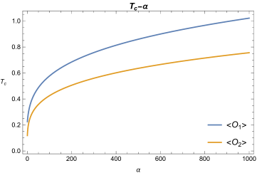
Figure 1: The critical temperature $T_{c}$ as a function of the coupling $\alpha$ for the condensates $\left\langle\mathcal{O}_{1}\right\rangle$ and $\left\langle\mathcal{O}_{2}\right\rangle$.

In this subsection, we numerically solve the equations $(\ref{eq:ansatz's EOM})$ with the boundary conditions discussed in Section II. We find that there exists a critical temperature $T_{c}$ associated with the holographic superconducting phase transition in the dual CFT. Above the critical temperature the condensate is zero while below the temperature the condensate occurs and the superconducting state in the boundary forms. We plot the critical temperature $T_{c}$ as a function of the coupling $\alpha$ in Fig. 1 and show that $T_{c}$ increases as $\alpha$ increases, which means that the non-minimal coupling of the scalar and the electromagnetic fields make the occurrence of the condensate easier. In other words, holographic superconductors have a higher superconducting transition temperature in the model with a larger coupling $\alpha$.

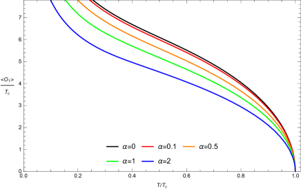
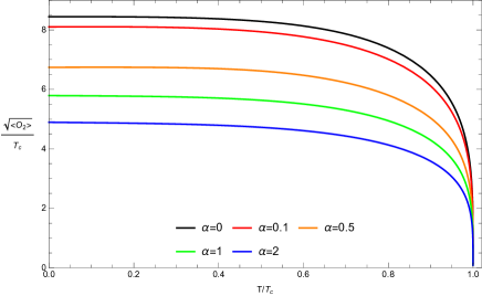
Figure 2: The condensates of the scalar field as a function of the temperature $T/T_{c}$ for various couplings $\alpha=0,0.1,0.5,1$ and $2$. Left Panel: The condensate of the operator $\mathcal{O}_{1}$. Right panel: The condensate of the operator $\mathcal{O}_{2}$.

$\alpha$	0	0.1	0.5	1	2	5	10
$2\times gap/T_{c}$	8.44	8.10	6.74	5.78	4.88	3.88	3.25

Table 1: The gaps of condensates $\left\langle\mathcal{O}_{2}\right\rangle$, which become smaller as $\alpha$ becomes larger.

In Fig. 2, we plot the condensates $\left\langle\mathcal{O}_{1}\right\rangle$ and $\left\langle\mathcal{O}_{2}\right\rangle$ as a function of the temperature $T$ for various couplings $\alpha$ in the left and right panels, respectively. It is obvious that the condensates only occur below the critical temperature $T_{c}$, and the curves with $\alpha=0$ recover the results in [8]. The condensates of different couplings $\alpha$ have similar increasing trends with the decrease of temperature in the both $\left\langle\mathcal{O}_{1}\right\rangle$ and $\left\langle\mathcal{O}_{2}\right\rangle$ cases. Moreover, the condensate is smaller for a larger $\alpha$, which implies that a stronger nonlinear coupling between the scalar and electromagnetic fields makes the scalar hair easier to be developed. Fitting the curves near the critical temperature $T_{c}$ for $\left\langle\mathcal{O}_{1}\right\rangle$ and $\left\langle\mathcal{O}_{2}\right\rangle$, we find that the condensates behave as $\left\langle\mathcal{O}_{i}\right\rangle\sim\left(1-T/T_{c}\right)^{1/2}$ for all values of $\alpha$. It is noteworthy that the condensate $\left\langle\mathcal{O}_{1}\right\rangle$ diverges as $T\rightarrow 0$, which means strong backreactions on the background metric. Therefore, at extremely low temperature, the probe limit is not a good approximation, and one may need to solve the full Einstein equation with backreactions [9]. Unlike $\left\langle\mathcal{O}_{1}\right\rangle$, the condensate $\left\langle\mathcal{O}_{2}\right\rangle$ approaches a constant as $T\rightarrow 0$. Actually, one can interpret the value of $\left\langle\mathcal{O}_{2}\right\rangle$ at $T=0$ as twice the superconducting gap, which is predicted to be $2\times$gap $=3.5T_{c}$ in BCS theory [4]. We list the superconducting gaps for various couplings $\alpha$ in Table 1, which shows that the superconducting gap becomes smaller as the coupling $\alpha$ becomes larger, and the range of the gaps recovers that of the high $T_{c}$ superconductors.

III.2 Conductivity

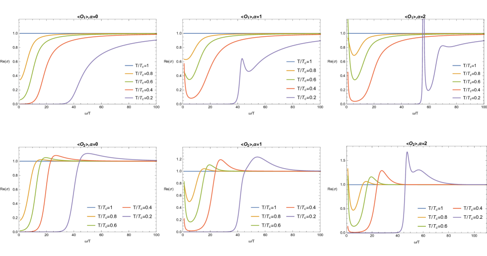
Figure 3: The real part of the conductivity $\operatorname{Re}\left(\sigma\right)$ as a function of $\omega/T$ for various $T/T_{c}$ with $\alpha=0$, $1$ and $2$. Upper row: Condensating $\mathcal{O}_{1}$. Bottom row: Condensating $\mathcal{O}_{2}$.

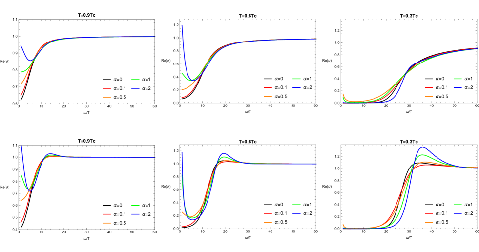
Figure 4: The real part of the conductivity $\operatorname{Re}\left(\sigma\right)$ as a function of $\omega/T$ for $\alpha=0,0.1,0.5,1$ and $2$ with a fixed temperature. The upper and bottom rows depict $\operatorname{Re}\left(\sigma\right)$ for condensating $\mathcal{O}_{1}$ and $\mathcal{O}_{2}$, respectively. The temperatures from the left column to the right one are $0.9T_{c}$, $0.6T_{c}$ and $0.3T_{c}$, respectively.

In this subsection, we investigate the optical conductivity in the dual CFT by solving equation $\left(\ref{eq:fluctuations' eq}\right)$. In Fig. 3, we plot the real part of the conductivity $\operatorname{Re}\left(\sigma\right)$ versus the frequency of fluctuations with $\alpha=0$, $1$ and $2$ in the both $\left\langle\mathcal{O}_{1}\right\rangle$ and $\left\langle\mathcal{O}_{2}\right\rangle$ cases. Note that the left column shows the $\alpha=0$ profiles, which recovers the results of [8]. The upper row of Fig. 3 displays the conductivity for condensating $\mathcal{O}_{1}$, while the bottom one presents the conductivity for condensating $\mathcal{O}_{2}$. The horizontal blue lines correspond to the frequency-independent conductivity at the critical temperature, which means that there is no condensate, and the system is dual to a metal-like matter in the boundary. As one lowers the temperature below $T_{c}$, a gap opens up and gets deeper. It is noteworthy that a spike appears inside the gap at a low enough temperature. Particularly in the $\alpha=2$ case of condensating $\mathcal{O}_{1}$, the spike behaves like a delta function, which will be discussed later. To better illustrate the effect of the coupling $\alpha$ on the conductivity, we plot $\operatorname{Re}\left(\sigma\right)$ as a function of $\omega/T$ for a given $T/T_{c}$ in Fig. 4. In the upper/bottom row of Fig. 4, the real part of the conductivity is plotted for condensating $\mathcal{O}_{1}$/$\mathcal{O}_{2}$. When the temperature is close to the critical temperature, e.g., $T=0.9T_{c}$, the gap is shallower for a larger $\alpha$, indicating a larger $\operatorname{Re}\left(\sigma\right)$. However, at a lower enough temperature, the gap becomes significantly deep regardless of the values of $\alpha$.

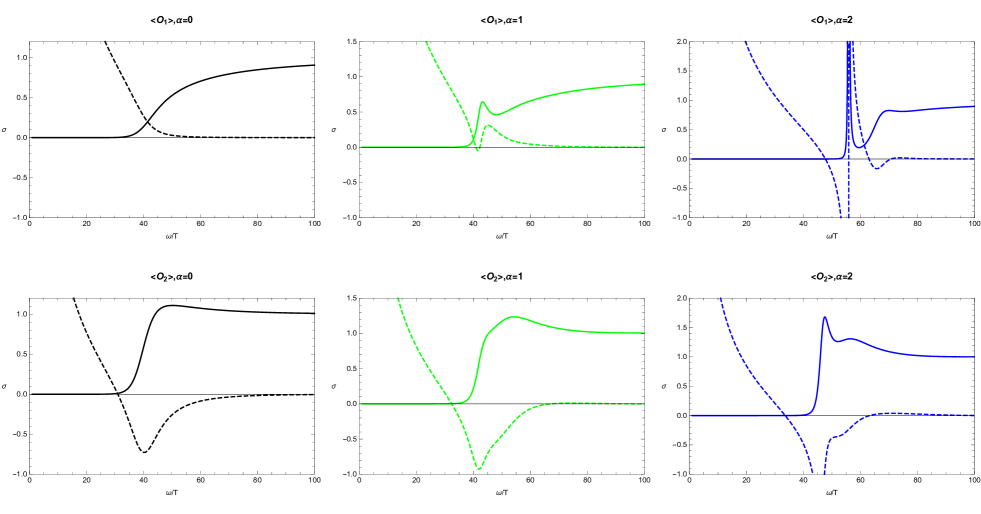
Figure 5: The real and imaginary parts of the conductivity for $\alpha=0,1,2$ at the temperature $T=0.2T_{c}$. The solid and the dashed lines represent the real and imaginary parts of the conductivity $\sigma(\omega)$, respectively.

It is well-known that $\operatorname{Re}\left(\sigma\right)$ has a delta function at $\omega=0$, which is not plotted in the above figures. Although the delta function can not be obtained directly from the numerical solution of $\operatorname{Re}\left(\sigma\right)$, it can be verified from $\operatorname{Im}\left(\sigma\right)$ according to the Kramers-Kronig relation

$$\operatorname{Im}\left[\sigma\left(\omega\right)\right]=-\frac{1}{\pi}\mathcal{P}\int_{-\infty}^{\infty}\frac{\operatorname{Re}\left[\sigma\left(\omega^{\prime}\right)\right]}{\omega^{\prime}-\omega}d\omega^{\prime}.$$ (17)

The real part of the conductivity has the form $\operatorname{Re}\left[\sigma\left(\omega\right)\right]\sim\pi n_{s}\delta\left(\omega\right)$, if the imaginary part of the conductivity has a pole, $\operatorname{Im}\left[\sigma\left(\omega\right)\right]\sim n_{s}/\omega$, where the coefficient $n_{s}$ is the superfluid density. Therefore, one can roughly observe the poles by examining the numerical results of the imaginary part of the conductivity as shown in Fig. 5. In Fig. 5, we plot the real and imaginary parts of the conductivity at a low temperature $T=0.2T_{c}$ by solid and dashed lines, respectively. The real part of the conductivity all shows a deep gap, which can be characterized by a gap frequency $\omega_{g}$, defined as the minimum point of the imaginary part of the conductivity. In the unit of the critical temperature $T_{c}$, the range of $\omega_{g}/T_{c}$ is approximately $8$ to $11$ for the three cases in Fig. 5. We also find that the gap frequency $\omega_{g}/T_{c}$ is getting larger as the coupling $\alpha$ increases. Note that the spike occurs in the case with the $\left\langle\mathcal{O}_{1}\right\rangle$ condensation and $\alpha=2$. This spike behaves like a delta function and is dictated by a pole of the imaginary part of conductivity. The occurrence of the spike corresponds to the interference of reflected and incident waves when the potential is high enough [10, 85]. Similar spikes are also observed in other models [28, 29].

IV Conclusions

In this paper, we investigated the holographic superconductor which is dual to the EMS model coupled with a charged scalar field in the asymptotically AdS spacetime. We focused on a non-minimal coupling function $h\left(\Psi\right)=e^{\alpha\Psi^{2}}$, which can lead to the spontaneous scalarization of black holes. The properties of scalarized black holes have been studied in [86, 87]. For simplicity, we studied the holographic superconductor in the probe limit, which means the matter fields do not backreact the background metric, but remains most of the interesting physics.

We first numerically solved the condensates of the scalar fields for the operators $\mathcal{O}_{1}$ and $\mathcal{O}_{2}$, which are due to the choice of the fall off $\Psi^{(1)}=0$ and $\Psi^{(2)}=0$, respectively. It showed that the operators only condense when the temperature is below the critical value $T_{c}$. By computing the critical temperatures $T_{c}$ of different couplings $\alpha$, we found that the critical temperature $T_{c}$ grows with the increase of $\alpha$. This result indicates that the effect of non-minimal coupling can raise the critical temperature of the holographic superconductor, which may provide an inspiration for high temperature superconductivity. We next discussed the optical conductivity of the superconductor. The real part of the conductivity is a constant when the temperature is above the critical value $T_{c}$, which behaves like a metal in the normal phase. As the temperature is lowered below the critical temperature, a gap is developed. One can characterize the gap by the gap frequency $\omega_{g}/T_{c}$, which gets larger as the coupling $\alpha$ increase. Interestingly, some spikes were shown to occur in the gap for some large coupling $\alpha$ at a low temperature. These spikes are associated with the interference of the reflected wave and the incident wave when the potential is high enough. Moreover, we found that the non-minimal coupling tends to make the spike occur since the spike is observed at a higher temperature at a larger coupling $\alpha$. Although the qualitative properties of holographic superconductors can be obtained in the probe limit, it is always desirable to investigate backreactions on the background metric. We leave this for future work.

- [1] Dirk van Delft and Peter Kes. The discovery of superconductivity. Physics Today, 63(9):38–43, sep 2010. doi:10.1063/1.3490499.
- [2] V. L. Ginzburg and L. D. Landau. On the Theory of superconductivity. Zh. Eksp. Teor. Fiz., 20:1064–1082, 1950.
- [3] J. Bardeen, L. N. Cooper, and J. R. Schrieffer. Microscopic theory of superconductivity. Physical Review, 106(1):162–164, apr 1957. doi:10.1103/physrev.106.162.
- [4] J. Bardeen, L. N. Cooper, and J. R. Schrieffer. Theory of superconductivity. Physical Review, 108(5):1175–1204, dec 1957. doi:10.1103/physrev.108.1175.
- [5] Elliot Snider, Nathan Dasenbrock-Gammon, Raymond McBride, Mathew Debessai, Hiranya Vindana, Kevin Vencatasamy, Keith V. Lawler, Ashkan Salamat, and Ranga P. Dias. Room-temperature superconductivity in a carbonaceous sulfur hydride. Nature, 586(7829):373–377, oct 2020. doi:10.1038/s41586-020-2801-z.
- [6] Juan Martin Maldacena. The Large N limit of superconformal field theories and supergravity. Int. J. Theor. Phys., 38:1113–1133, 1999. arXiv:hep-th/9711200, doi:10.1023/A:1026654312961.
- [7] Steven S. Gubser. Breaking an Abelian gauge symmetry near a black hole horizon. Phys. Rev. D, 78:065034, 2008. arXiv:0801.2977, doi:10.1103/PhysRevD.78.065034.
- [8] Sean A. Hartnoll, Christopher P. Herzog, and Gary T. Horowitz. Building a Holographic Superconductor. Phys. Rev. Lett., 101:031601, 2008. arXiv:0803.3295, doi:10.1103/PhysRevLett.101.031601.
- [9] Sean A. Hartnoll, Christopher P. Herzog, and Gary T. Horowitz. Holographic Superconductors. JHEP, 12:015, 2008. arXiv:0810.1563, doi:10.1088/1126-6708/2008/12/015.
- [10] Gary T. Horowitz and Matthew M. Roberts. Holographic Superconductors with Various Condensates. Phys. Rev. D, 78:126008, 2008. arXiv:0810.1077, doi:10.1103/PhysRevD.78.126008.
- [11] Yves Brihaye and Betti Hartmann. Holographic Superconductors in 3+1 dimensions away from the probe limit. Phys. Rev. D, 81:126008, 2010. arXiv:1003.5130, doi:10.1103/PhysRevD.81.126008.
- [12] Steven S Gubser and Silviu S Pufu. The gravity dual of a p-wave superconductor. Journal of High Energy Physics, 2008(11):033–033, nov 2008. doi:10.1088/1126-6708/2008/11/033.
- [13] Rong-Gen Cai, Zhang-Yu Nie, and Hai-Qing Zhang. Holographic p-wave superconductors from Gauss-Bonnet gravity. Phys. Rev. D, 82:066007, 2010. arXiv:1007.3321, doi:10.1103/PhysRevD.82.066007.
- [14] Jiunn-Wei Chen, Ying-Jer Kao, Debaprasad Maity, Wen-Yu Wen, and Chen-Pin Yeh. Towards A Holographic Model of D-Wave Superconductors. Phys. Rev. D, 81:106008, 2010. arXiv:1003.2991, doi:10.1103/PhysRevD.81.106008.
- [15] Francesco Benini, Christopher P. Herzog, Rakibur Rahman, and Amos Yarom. Gauge gravity duality for d-wave superconductors: prospects and challenges. JHEP, 11:137, 2010. arXiv:1007.1981, doi:10.1007/JHEP11(2010)137.
- [16] Keun-Young Kim and Marika Taylor. Holographic d-wave superconductors. JHEP, 08:112, 2013. arXiv:1304.6729, doi:10.1007/JHEP08(2013)112.
- [17] Rong-Gen Cai, Li Li, and Li-Fang Li. A Holographic P-wave Superconductor Model. JHEP, 01:032, 2014. arXiv:1309.4877, doi:10.1007/JHEP01(2014)032.
- [18] Oriol Domenech, Marc Montull, Alex Pomarol, Alberto Salvio, and Pedro J. Silva. Emergent Gauge Fields in Holographic Superconductors. JHEP, 08:033, 2010. arXiv:1005.1776, doi:10.1007/JHEP08(2010)033.
- [19] Marc Montull, Oriol Pujolas, Alberto Salvio, and Pedro J. Silva. Magnetic Response in the Holographic Insulator/Superconductor Transition. JHEP, 04:135, 2012. arXiv:1202.0006, doi:10.1007/JHEP04(2012)135.
- [20] Alberto Salvio. Holographic superfluids and superconductors in dilaton-gravity. Journal of High Energy Physics, 2012(9), sep 2012. doi:10.1007/jhep09(2012)134.
- [21] Jiliang Jing and Songbai Chen. Holographic superconductors in the Born-Infeld electrodynamics. Phys. Lett. B, 686:68–71, 2010. arXiv:1001.4227, doi:10.1016/j.physletb.2010.02.022.
- [22] Jiliang Jing, Qiyuan Pan, and Songbai Chen. Holographic Superconductors with Power-Maxwell field. JHEP, 11:045, 2011. arXiv:1106.5181, doi:10.1007/JHEP11(2011)045.
- [23] Sunandan Gangopadhyay and Dibakar Roychowdhury. Analytic study of properties of holographic superconductors in Born-Infeld electrodynamics. JHEP, 05:002, 2012. arXiv:1201.6520, doi:10.1007/JHEP05(2012)002.
- [24] Sunandan Gangopadhyay and Dibakar Roychowdhury. Analytic study of Gauss-Bonnet holographic superconductors in Born-Infeld electrodynamics. JHEP, 05:156, 2012. arXiv:1204.0673, doi:10.1007/JHEP05(2012)156.
- [25] Benrong Mu, Peng Wang, and Haitang Yang. Holographic DC Conductivity for a Power-law Maxwell Field. Eur. Phys. J. C, 78(12):1005, 2018. arXiv:1711.06569, doi:10.1140/epjc/s10052-018-6491-8.
- [26] Peng Wang, Houwen Wu, and Haitang Yang. Holographic DC Conductivity for Backreacted Nonlinear Electrodynamics with Momentum Dissipation. Eur. Phys. J. C, 79(1):6, 2019. arXiv:1805.07913, doi:10.1140/epjc/s10052-018-6503-8.
- [27] Ruth Gregory, Sugumi Kanno, and Jiro Soda. Holographic Superconductors with Higher Curvature Corrections. JHEP, 10:010, 2009. arXiv:0907.3203, doi:10.1088/1126-6708/2009/10/010.
- [28] Qiyuan Pan, Bin Wang, Eleftherios Papantonopoulos, J. Oliveira, and A. B. Pavan. Holographic Superconductors with various condensates in Einstein-Gauss-Bonnet gravity. Phys. Rev. D, 81:106007, 2010. arXiv:0912.2475, doi:10.1103/PhysRevD.81.106007.
- [29] Qiyuan Pan and Bin Wang. General holographic superconductor models with Gauss-Bonnet corrections. Phys. Lett. B, 693:159–165, 2010. arXiv:1005.4743, doi:10.1016/j.physletb.2010.08.017.
- [30] Tameem Albash and Clifford V. Johnson. A Holographic Superconductor in an External Magnetic Field. JHEP, 09:121, 2008. arXiv:0804.3466, doi:10.1088/1126-6708/2008/09/121.
- [31] Xian-Hui Ge, Bin Wang, Shao-Feng Wu, and Guo-Hong Yang. Analytical study on holographic superconductors in external magnetic field. JHEP, 08:108, 2010. arXiv:1002.4901, doi:10.1007/JHEP08(2010)108.
- [32] Martin Ammon, Johanna Erdmenger, Matthias Kaminski, and Patrick Kerner. Superconductivity from gauge/gravity duality with flavor. Phys. Lett. B, 680:516–520, 2009. arXiv:0810.2316, doi:10.1016/j.physletb.2009.09.029.
- [33] Martin Ammon, Johanna Erdmenger, Matthias Kaminski, and Patrick Kerner. Flavor Superconductivity from Gauge/Gravity Duality. JHEP, 10:067, 2009. arXiv:0903.1864, doi:10.1088/1126-6708/2009/10/067.
- [34] Matthias Kaminski. Flavor Superconductivity & Superfluidity. Lect. Notes Phys., 828:349–393, 2011. arXiv:1002.4886, doi:10.1007/978-3-642-04864-7_11.
- [35] Tameem Albash and Clifford V. Johnson. Vortex and Droplet Engineering in Holographic Superconductors. Phys. Rev. D, 80:126009, 2009. arXiv:0906.1795, doi:10.1103/PhysRevD.80.126009.
- [36] Óscar J. C. Dias, Gary T. Horowitz, Nabil Iqbal, and Jorge E. Santos. Vortices in holographic superfluids and superconductors as conformal defects. JHEP, 04:096, 2014. arXiv:1311.3673, doi:10.1007/JHEP04(2014)096.
- [37] Irene Amado, Matthias Kaminski, and Karl Landsteiner. Hydrodynamics of Holographic Superconductors. JHEP, 05:021, 2009. arXiv:0903.2209, doi:10.1088/1126-6708/2009/05/021.
- [38] Tameem Albash and Clifford V. Johnson. Holographic Studies of Entanglement Entropy in Superconductors. JHEP, 05:079, 2012. arXiv:1202.2605, doi:10.1007/JHEP05(2012)079.
- [39] Gary T. Horowitz and Matthew M. Roberts. Zero Temperature Limit of Holographic Superconductors. JHEP, 11:015, 2009. arXiv:0908.3677, doi:10.1088/1126-6708/2009/11/015.
- [40] Tatsuma Nishioka, Shinsei Ryu, and Tadashi Takayanagi. Holographic Superconductor/Insulator Transition at Zero Temperature. JHEP, 03:131, 2010. arXiv:0911.0962, doi:10.1007/JHEP03(2010)131.
- [41] R. A. Konoplya and A. Zhidenko. Holographic conductivity of zero temperature superconductors. Phys. Lett. B, 686:199–206, 2010. arXiv:0909.2138, doi:10.1016/j.physletb.2010.02.048.
- [42] E. J. Brynjolfsson, U. H. Danielsson, L. Thorlacius, and T. Zingg. Holographic Superconductors with Lifshitz Scaling. J. Phys. A, 43:065401, 2010. arXiv:0908.2611, doi:10.1088/1751-8113/43/6/065401.
- [43] Jun-Wang Lu, Ya-Bo Wu, Peng Qian, Yue-Yue Zhao, and Xue Zhang. Lifshitz Scaling Effects on Holographic Superconductors. Nucl. Phys. B, 887:112–135, 2014. arXiv:1311.2699, doi:10.1016/j.nuclphysb.2014.08.001.
- [44] Gary T. Horowitz, Jorge E. Santos, and Benson Way. A Holographic Josephson Junction. Phys. Rev. Lett., 106:221601, 2011. arXiv:1101.3326, doi:10.1103/PhysRevLett.106.221601.
- [45] Yong-Qiang Wang, Yu-Xiao Liu, Rong-Gen Cai, Shingo Takeuchi, and Hai-Qing Zhang. Holographic SIS Josephson Junction. JHEP, 09:058, 2012. arXiv:1205.4406, doi:10.1007/JHEP09(2012)058.
- [46] Ya-Peng Hu, Huai-Fan Li, Hua-Bi Zeng, and Hai-Qing Zhang. Holographic Josephson Junction from Massive Gravity. Phys. Rev. D, 93(10):104009, 2016. arXiv:1512.07035, doi:10.1103/PhysRevD.93.104009.
- [47] Thibault Damour and Gilles Esposito-Farese. Nonperturbative strong field effects in tensor - scalar theories of gravitation. Phys. Rev. Lett., 70:2220–2223, 1993. doi:10.1103/PhysRevLett.70.2220.
- [48] Vitor Cardoso, Isabella P. Carucci, Paolo Pani, and Thomas P. Sotiriou. Matter around Kerr black holes in scalar-tensor theories: scalarization and superradiant instability. Phys. Rev. D, 88:044056, 2013. arXiv:1305.6936, doi:10.1103/PhysRevD.88.044056.
- [49] Vitor Cardoso, Isabella P. Carucci, Paolo Pani, and Thomas P. Sotiriou. Black holes with surrounding matter in scalar-tensor theories. Phys. Rev. Lett., 111:111101, 2013. arXiv:1308.6587, doi:10.1103/PhysRevLett.111.111101.
- [50] Daniela D. Doneva and Stoytcho S. Yazadjiev. New Gauss-Bonnet Black Holes with Curvature-Induced Scalarization in Extended Scalar-Tensor Theories. Phys. Rev. Lett., 120(13):131103, 2018. arXiv:1711.01187, doi:10.1103/PhysRevLett.120.131103.
- [51] Hector O. Silva, Jeremy Sakstein, Leonardo Gualtieri, Thomas P. Sotiriou, and Emanuele Berti. Spontaneous scalarization of black holes and compact stars from a Gauss-Bonnet coupling. Phys. Rev. Lett., 120(13):131104, 2018. arXiv:1711.02080, doi:10.1103/PhysRevLett.120.131104.
- [52] G. Antoniou, A. Bakopoulos, and P. Kanti. Evasion of No-Hair Theorems and Novel Black-Hole Solutions in Gauss-Bonnet Theories. Phys. Rev. Lett., 120(13):131102, 2018. arXiv:1711.03390, doi:10.1103/PhysRevLett.120.131102.
- [53] Pedro V.P. Cunha, Carlos A.R. Herdeiro, and Eugen Radu. Spontaneously Scalarized Kerr Black Holes in Extended Scalar-Tensor–Gauss-Bonnet Gravity. Phys. Rev. Lett., 123(1):011101, 2019. arXiv:1904.09997, doi:10.1103/PhysRevLett.123.011101.
- [54] Carlos A. R. Herdeiro, Eugen Radu, Hector O. Silva, Thomas P. Sotiriou, and Nicolás Yunes. Spin-induced scalarized black holes. Phys. Rev. Lett., 126(1):011103, 2021. arXiv:2009.03904, doi:10.1103/PhysRevLett.126.011103.
- [55] Emanuele Berti, Lucas G. Collodel, Burkhard Kleihaus, and Jutta Kunz. Spin-induced black-hole scalarization in Einstein-scalar-Gauss-Bonnet theory. Phys. Rev. Lett., 126(1):011104, 2021. arXiv:2009.03905, doi:10.1103/PhysRevLett.126.011104.
- [56] Yves Brihaye, Betti Hartmann, Nathália Pio Aprile, and Jon Urrestilla. Scalarization of asymptotically anti–de Sitter black holes with applications to holographic phase transitions. Phys. Rev. D, 101(12):124016, 2020. arXiv:1911.01950, doi:10.1103/PhysRevD.101.124016.
- [57] Carlos A.R. Herdeiro, Eugen Radu, Nicolas Sanchis-Gual, and José A. Font. Spontaneous Scalarization of Charged Black Holes. Phys. Rev. Lett., 121(10):101102, 2018. arXiv:1806.05190, doi:10.1103/PhysRevLett.121.101102.
- [58] Pedro G. S. Fernandes, Carlos A. R. Herdeiro, Alexandre M. Pombo, Eugen Radu, and Nicolas Sanchis-Gual. Spontaneous Scalarisation of Charged Black Holes: Coupling Dependence and Dynamical Features. Class. Quant. Grav., 36(13):134002, 2019. [Erratum: Class.Quant.Grav. 37, 049501 (2020)]. arXiv:1902.05079, doi:10.1088/1361-6382/ab23a1.
- [59] Jose Luis Blázquez-Salcedo, Carlos A.R. Herdeiro, Jutta Kunz, Alexandre M. Pombo, and Eugen Radu. Einstein-Maxwell-scalar black holes: the hot, the cold and the bald. Phys. Lett. B, 806:135493, 2020. arXiv:2002.00963, doi:10.1016/j.physletb.2020.135493.
- [60] D. Astefanesei, C. Herdeiro, A. Pombo, and E. Radu. Einstein-Maxwell-scalar black holes: classes of solutions, dyons and extremality. JHEP, 10:078, 2019. arXiv:1905.08304, doi:10.1007/JHEP10(2019)078.
- [61] Pedro G.S. Fernandes, Carlos A.R. Herdeiro, Alexandre M. Pombo, Eugen Radu, and Nicolas Sanchis-Gual. Charged black holes with axionic-type couplings: Classes of solutions and dynamical scalarization. Phys. Rev. D, 100(8):084045, 2019. arXiv:1908.00037, doi:10.1103/PhysRevD.100.084045.
- [62] De-Cheng Zou and Yun Soo Myung. Scalarized charged black holes with scalar mass term. Phys. Rev. D, 100(12):124055, 2019. arXiv:1909.11859, doi:10.1103/PhysRevD.100.124055.
- [63] Pedro G.S. Fernandes. Einstein-Maxwell-scalar black holes with massive and self-interacting scalar hair. Phys. Dark Univ., 30:100716, 2020. arXiv:2003.01045, doi:10.1016/j.dark.2020.100716.
- [64] Yan Peng. Scalarization of horizonless reflecting stars: neutral scalar fields non-minimally coupled to Maxwell fields. Phys. Lett. B, 804:135372, 2020. arXiv:1912.11989, doi:10.1016/j.physletb.2020.135372.
- [65] Yun Soo Myung and De-Cheng Zou. Instability of Reissner–Nordström black hole in Einstein-Maxwell-scalar theory. Eur. Phys. J. C, 79(3):273, 2019. arXiv:1808.02609, doi:10.1140/epjc/s10052-019-6792-6.
- [66] Yun Soo Myung and De-Cheng Zou. Stability of scalarized charged black holes in the Einstein–Maxwell–Scalar theory. Eur. Phys. J. C, 79(8):641, 2019. arXiv:1904.09864, doi:10.1140/epjc/s10052-019-7176-7.
- [67] De-Cheng Zou and Yun Soo Myung. Radial perturbations of the scalarized black holes in Einstein-Maxwell-conformally coupled scalar theory. Phys. Rev. D, 102(6):064011, 2020. arXiv:2005.06677, doi:10.1103/PhysRevD.102.064011.
- [68] Yun Soo Myung and De-Cheng Zou. Onset of rotating scalarized black holes in Einstein-Chern-Simons-Scalar theory. Phys. Lett. B, 814:136081, 2021. arXiv:2012.02375, doi:10.1016/j.physletb.2021.136081.
- [69] Zhan-Feng Mai and Run-Qiu Yang. Stability analysis on charged black hole with non-linear complex scalar. 12 2020. arXiv:2101.00026.
- [70] Dumitru Astefanesei, Carlos Herdeiro, João Oliveira, and Eugen Radu. Higher dimensional black hole scalarization. JHEP, 09:186, 2020. arXiv:2007.04153, doi:10.1007/JHEP09(2020)186.
- [71] Yun Soo Myung and De-Cheng Zou. Quasinormal modes of scalarized black holes in the Einstein–Maxwell–Scalar theory. Phys. Lett. B, 790:400–407, 2019. arXiv:1812.03604, doi:10.1016/j.physletb.2019.01.046.
- [72] Jose Luis Blázquez-Salcedo, Carlos A.R. Herdeiro, Sarah Kahlen, Jutta Kunz, Alexandre M. Pombo, and Eugen Radu. Quasinormal modes of hot, cold and bald Einstein-Maxwell-scalar black holes. 8 2020. arXiv:2008.11744.
- [73] Yun Soo Myung and De-Cheng Zou. Scalarized charged black holes in the Einstein-Maxwell-Scalar theory with two U(1) fields. Phys. Lett. B, 811:135905, 2020. arXiv:2009.05193, doi:10.1016/j.physletb.2020.135905.
- [74] Yun Soo Myung and De-Cheng Zou. Scalarized black holes in the Einstein-Maxwell-scalar theory with a quasitopological term. Phys. Rev. D, 103(2):024010, 2021. arXiv:2011.09665, doi:10.1103/PhysRevD.103.024010.
- [75] Hong Guo, Xiao-Mei Kuang, Eleftherios Papantonopoulos, and Bin Wang. Topology and spacetime structure influences on black hole scalarization. 12 2020. arXiv:2012.11844.
- [76] Peng Wang, Houwen Wu, and Haitang Yang. Scalarized Einstein-Born-Infeld-scalar Black Holes. 12 2020. arXiv:2012.01066.
- [77] R. A. Konoplya and A. Zhidenko. Analytical representation for metrics of scalarized Einstein-Maxwell black holes and their shadows. Phys. Rev. D, 100(4):044015, 2019. arXiv:1907.05551, doi:10.1103/PhysRevD.100.044015.
- [78] Yves Brihaye, Carlos Herdeiro, and Eugen Radu. Black Hole Spontaneous Scalarisation with a Positive Cosmological Constant. Phys. Lett. B, 802:135269, 2020. arXiv:1910.05286, doi:10.1016/j.physletb.2020.135269.
- [79] Shahar Hod. Spontaneous scalarization of charged Reissner-Nordstr\”om black holes: Analytic treatment along the existence line. Phys. Lett. B, 798:135025, 2019. arXiv:2002.01948.
- [80] Shahar Hod. Reissner-Nordström black holes supporting nonminimally coupled massive scalar field configurations. Phys. Rev. D, 101(10):104025, 2020. arXiv:2005.10268, doi:10.1103/PhysRevD.101.104025.
- [81] Shahar Hod. Analytic treatment of near-extremal charged black holes supporting non-minimally coupled massless scalar clouds. Eur. Phys. J. C, 80(12):1150, 2020. doi:10.1140/epjc/s10052-020-08723-z.
- [82] Subhash Mahapatra, Supragyan Priyadarshinee, Gosala Narasimha Reddy, and Bhaskar Shukla. Exact topological charged hairy black holes in AdS Space in -dimensions. Phys. Rev. D, 102(2):024042, 2020. arXiv:2004.00921, doi:10.1103/PhysRevD.102.024042.
- [83] Qingyu Gan, Peng Wang, Houwen Wu, and Haitang Yang. Photon ring and observational appearance of a hairy black hole. Phys. Rev. D, 104(4):044049, 2021. arXiv:2105.11770, doi:10.1103/PhysRevD.104.044049.
- [84] Qingyu Gan, Peng Wang, Houwen Wu, and Haitang Yang. Photon spheres and spherical accretion image of a hairy black hole. Phys. Rev. D, 104(2):024003, 2021. arXiv:2104.08703, doi:10.1103/PhysRevD.104.024003.
- [85] Gary T. Horowitz. Introduction to Holographic Superconductors. Lect. Notes Phys., 828:313–347, 2011. arXiv:1002.1722, doi:10.1007/978-3-642-04864-7_10.
- [86] Guangzhou Guo, Peng Wang, Houwen Wu, and Haitang Yang. Scalarized Einstein–Maxwell-scalar black holes in anti-de Sitter spacetime. Eur. Phys. J. C, 81(10):864, 2021. arXiv:2102.04015, doi:10.1140/epjc/s10052-021-09614-7.
- [87] Guangzhou Guo, Peng Wang, Houwen Wu, and Haitang Yang. Thermodynamics and Phase Structure of an Einstein-Maxwell-scalar Model in Extended Phase Space. 7 2021. arXiv:2107.04467.