Experimental demonstration of coherence flow in $\mathcal{PT}$- and anti-$\mathcal{PT}$-symmetric systems

Abstract

Abstract

Non-Hermitian parity-time ($\mathcal{PT}$) and anti-parity-time ($\mathcal{APT}$)-symmetric systems exhibit novel quantum properties and have attracted increasing interest. Although many counterintuitive phenomena in $\mathcal{PT}$- and $\mathcal{APT}$-symmetric systems were previously studied, coherence flow has been rarely investigated. Here, we experimentally demonstrate single-qubit coherence flow in $\mathcal{PT}$- and $\mathcal{APT}$-symmetric systems using an optical setup. In the symmetry unbroken regime, we observe different periodic oscillations of coherence. Particularly, we observe two complete coherence backflows in one period in the $\mathcal{PT}$-symmetric system, while only one backflow in the $\mathcal{APT}$-symmetric system. Moreover, in the symmetry broken regime, we observe the phenomenon of stable value of coherence flow. We derive the analytic proofs of these phenomena and show that most experimental data agree with theoretical results within one standard deviation. This work opens avenues for future study on the dynamics of coherence in $\mathcal{PT}$- and $\mathcal{APT}$-symmetric systems.

I Introduction

Non-Hermitian Hamiltonians, satisfying parity-time ($\mathcal{PT}$) symmetry, can have real eigenvalues in the symmetry unbroken zone cm ; Konotop ; Ganainy . A $\mathcal{PT}$-symmetric Hamiltonian satisfies $[\hat{H},\hat{\mathcal{P}}\hat{\mathcal{T}}]=0$, with the joint parity-time operator ($\hat{\mathcal{P}}\hat{\mathcal{T}}$). $\mathcal{PT}$-symmetric non-Hermitian Hamiltonians feature unconventional properties in numerous systems ranging from classical jsa040101 ; fk041805 ; YDchong ; ar167 ; LFeng ; BPengS ; HJS ; LeeYC ; cyju062118 ; bpsk394 ; iia053806 ; qjj1160 to quantum systems chgx083604 ; ZhangJ ; Ozdemir ; LiJ ; TangJS ; WangYT ; XiaoL2 ; FQU ; ZHBL2 ; iiaaf ; kka . When the Hamiltonian parameters cross the exceptional point (EP), $\mathcal{PT}$ symmetry is broken, leading to a symmetry-breaking transition. This has inspired a number of studies on many counterintuitive phenomena emerging in such systems.

Previous experiments demonstrated single-mode lasing or anti-lasing lfeng972 ; hhodaei975 , bistable lasing svsa18 , loss-induced transparency or lasing aguo103 ; BPengS , EP-enhanced sensing ZPL ; wchen192 ; hhodaei187 , and $\mathcal{PT}$ symmetry breaking Ozdemir ; aguo103 ; LiJ ; CER ; YangW . Moreover, recent experiments have observed: information flow in $\mathcal{PT}$-symmetric systems XiaoL2 , protection of quantum coherence in a $\mathcal{PT}$-broken superconducting circuit mnaghiloo1232 , EP-enhanced coherence and oscillation of coherence in a single ion $\mathcal{PT}$-symmetry system Chenpx , entanglement restoration in a $\mathcal{PT}$-symmetric system using a universal circuit LongGL1 , and dynamical features of a triple-qubit system in which one qubit evolves under a local $\mathcal{PT}$-symmetric Hamiltonian LongGL2 .

Another important counterpart, anti-$\mathcal{PT}$ ($\mathcal{APT}$) symmetry, has recently attracted considerable interest. $\mathcal{APT}$ symmetry means that the system Hamiltonian is anti-commutative with the joint $\mathcal{PT}$ operator, i.e., $\{\hat{H},\hat{\mathcal{P}}\hat{\mathcal{T}}\}=0$. $\mathcal{APT}$-symmetric systems exhibit noteworthy effects, such as balanced positive and negative index GeL , coherent switch VVKDA , and constant refraction YangF . Some relevant experimental demonstrations have been realized in optics VVKDA ; LiQ , atoms jhw033811 ; ppengwx1139 ; ylchuang21969 ; yjy193604 , electrical circuit resonators Choi , magnon-cavity hybrid systems jz014053 , and diffusive systems LiY . In addition, experiments have demonstrated $\mathcal{APT}$ symmetry breaking LiY ; HLZR , simulated $\mathcal{APT}$-symmetric Lorentz dynamics LiQ , and observed $\mathcal{APT}$ exceptional points Choi . Moreover, information flow in an $\mathcal{APT}$-symmetric system with nuclear spins has been observed in recent experiments Wen .

Although many counterintuitive phenomena in $\mathcal{PT}$- or $\mathcal{APT}$-symmetric systems were previously studied, the flow of coherence in $\mathcal{PT}$-symmetric systems has not been fully and thoroughly investigated. Moreover, the coherence flow in $\mathcal{APT}$-symmetric systems has not been studied either theoretically or experimentally. The study of coherence flow is interesting and meaningful because it can discover various phenomena different from Hermitian quantum mechanics and reveal the relationship between non-Hermitian systems and their environment.

In Hermitian quantum systems isolated from their environment, the coherence flow between the subsystems generally oscillates periodically over time, and the oscillation period depends on the coupling strength between the subsystems. Different from Hermitian quantum systems, most non-Hermitian physical systems typically involve gain and loss induced by the environment. In this case, the behavior of coherence flow in non-Hermitian physical systems is generally quite different from that of the coherence flow in Hermitian physical systems.

For example, the dissipative coupling between the system and the environment may disturb and even wash out quantum coherence. On the other hand, due to the gain effect, the coherence originally lost into the environment may return to the system, and thus oscillates periodically over time. By investigating the coherence flow between the system and its environment, one can obtain some important information, such as the coupling strength between systems and their environment, the type of environment (i.e., Markov or non-Markov environment), the presence of memory effects in the open quantum dynamics, etc..

In this study, we experimentally demonstrate the coherence flow of a single qubit in $\mathcal{PT}$- and $\mathcal{APT}$-symmetric systems using a simple optical setup. In the symmetry unbroken regime, we observe different periodic oscillations of coherence in both $\mathcal{PT}$- and $\mathcal{APT}$-symmetric systems. Double touch of coherence (DTC) (i.e., complete coherence backflow happening twice in one period) is revealed in the $\mathcal{PT}$-symmetric system, while only one backflow exists in the $\mathcal{APT}$-symmetric system. In addition, we observe the phenomenon of stable value (PSV) of coherence in the symmetry broken regime, which is independent of its initial state. Concretely, the coherence tends to a stable value $1/a$ in the $\mathcal{PT}$-symmetric system, but it approaches 1 in the $\mathcal{APT}$-symmetric system. We also provide the theoretical analytic proofs of these phenomena (see Supplementary Notes 1-4) and compare with previous relevant works. Our results imply that the coherence backflow and PSV are quite different for these two kinds of symmetric systems.

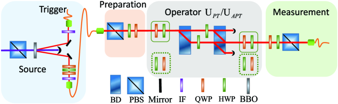
Fig.  1: Experimental setup. Blue area to the left: Pairs of 808 $\rm{nm}$ single photons are generated by passing a 404 $\rm{nm}$ laser light through a type-I spontaneous parametric down conversion, and using a nonlinear-barium-borate (BBO) crystal. Orange area: After photons pass through the $3$ $\rm{nm}$ interference filter (IF), one photon serves as a trigger and the other signal photon is prepared in an arbitrary linear polarization state. Grey area: Two sets of beam displacers (BDs), together with half-wave plates (HWPs) and quarter-wave plates (QWPs), are used to construct the operators $\boldsymbol{U}_{\mathcal{PT}}$ and $\boldsymbol{U}_{\mathcal{APT}}$. In the measurement part, the density matrix is constructed via quantum state tomography. PBS: polarization beam splitter.

II Results

Principle and setup of the experiment. A non-trivial general $\mathcal{PT}$-symmetric Hamiltonian for a single qubit takes the form LeeYC ; TangJS

$$\hat{H}_{\mathcal{PT}}=\left(\begin{array}[]{ll}i\gamma&s\\ s&-i\gamma\end{array}\right)=s(\hat{\sigma}_{x}+ia\hat{\sigma}_{z}).$$ (1)

While a generic $\mathcal{APT}$-symmetric Hamiltonian of a single qubit can be expressed as Wen ; LiY

$$\hat{H}_{\mathcal{APT}}=\left(\begin{array}[]{ll}\gamma&is\\ is&-\gamma\end{array}\right)=s(i\hat{\sigma}_{x}+a\hat{\sigma}_{z}).$$ (2)

Here, the parameter $s>0$ is an energy scale, $a=\gamma/s>0$ is a coefficient representing the degree of non-Hermiticity, $\hat{\sigma}_{x}$ and $\hat{\sigma}_{z}$ are the standard Pauli operators. In the $\mathcal{PT}$-symmetric system, the eigenvalue of $\hat{H}_{\mathcal{PT}}$ is

$$\lambda_{\mathcal{PT}}=\pm s\sqrt{1-a^{2}},$$ (3)

which is an imaginary number for $a>1$ (the $\mathcal{PT}$ symmetry broken regime), while a real number for $0<a<1$ (the $\mathcal{PT}$ symmetry unbroken regime). However, in the $\mathcal{APT}$-symmetric system, the eigenvalue of $\hat{H}_{\mathcal{APT}}$ is

$$\lambda_{\mathcal{APT}}=\pm s\sqrt{a^{2}-1},$$ (4)

which is an imaginary number for $0<a<1$ (the $\mathcal{APT}$ symmetry broken regime), while a real number for $a\!\!>\!\!1$ (the $\mathcal{APT}$ symmetry unbroken regime). Note that the eigenvalues of both Hamiltonians $\hat{H}_{\mathcal{PT}}$ and $\hat{H}_{\mathcal{APT}}$ are zero for $a=1$ (the exceptional point).
For different $s$, the time evolution of quantum states under the Hamiltonian $\hat{H}_{\mathcal{PT}}$ ($\hat{H}_{\mathcal{APT}}$) follows the same rules because $s$ is an energy scale. Therefore, without loss of generality, we consider $s=1$ for both $\hat{H}_{\mathcal{PT}}$ and $\hat{H}_{\mathcal{APT}}$ WangYT ; XiaoL2 . In our experiment, the non-unitary operators $\boldsymbol{U}_{\mathcal{PT}}=\mathrm{exp}(-i\hat{H}_{\mathcal{PT}}t)$ and $\boldsymbol{U}_{\mathcal{APT}}=\mathrm{exp}(-i\hat{H}_{\mathcal{APT}}t)$ are realized by XiaoL2 ; Stewart

$$\boldsymbol{U}_{\mathcal{PT}}= R_{\mathrm{HWP}}\left(\theta_{1}\right)R_{\mathrm{QWP}}\left(2\theta_{1}\right)L\left(\xi_{1},\xi_{2}\right)$$ (5)

$$R_{\mathrm{HWP}}\left(-\theta_{1}+\pi/4\right)R_{\mathrm{QWP}}\left(0\right),$$

$$\boldsymbol{U}_{\mathcal{APT}}= R_{\mathrm{QWP}}\left(0\right)R_{\mathrm{HWP}}\left(\pi/4\right)L\left(\xi_{3},\xi_{3}\right)$$ (6)

$$R_{\mathrm{QWP}}\left(\varphi_{1}\right)R_{\mathrm{HWP}}\left(\varphi_{2}\right),$$

where the loss-dependent operator

$$L\left(\xi_{i},\xi_{j}\right)=\left(\begin{array}[]{ll}0&\mathrm{sin}2\xi_{i}\\ \mathrm{sin}2\xi_{j}&0\end{array}\right)$$ (7)

is realized by a combination of two beam displacers (BDs) and two half-wave plates (HWPs) with setting angles $\xi_{i}$ and $\xi_{j}$ (see Supplementary Note 5) XiaoL2 . Above, $R_{\textrm{HWP}}$ and $R_{\textrm{QWP}}$ are the rotation operators of HWP and QWP (quarter wave plate), respectively. Here, the setting angles $(\theta_{1},\varphi_{1},\varphi_{2},\xi_{1},\xi_{2},\xi_{3})$ depend on the initial state and are determined numerically by reversal design for each given time $t$, according to the time-evolution operators $\boldsymbol{U}_{\mathcal{PT}}$ and $\boldsymbol{U}_{\mathcal{APT}}$.
The dynamical evolution of the quantum states in the $\mathcal{PT}$- or $\mathcal{APT}$-symmetric system is given by kka ; XiaoL2 ; Brody

$$\boldsymbol{\rho}(t)=\frac{\boldsymbol{U}(t)\boldsymbol{\rho}(0)\boldsymbol{U}^{\dagger}(t)}{\rm Tr\left[\boldsymbol{U}(t)\boldsymbol{\rho}(0)\boldsymbol{U}^{\dagger}(t)\right]},$$ (8)

where $\boldsymbol{U}(t)=\boldsymbol{U}_{\mathcal{PT}}(t)$ or $\boldsymbol{U}_{\mathcal{APT}}(t)$, $\boldsymbol{\rho}(0)$ is the initial density matrix, and $\boldsymbol{\rho}(t)$ is the density matrix at any given time $t$. Here, we use the $l_{1}$ norm of coherence Baumgratz ; Mani to quantify the coherence of $\boldsymbol{\rho}(t)$, i.e.,

$$C_{l_{1}}\left(\boldsymbol{\rho}(t)\right)=\sum_{i\neq j}\left|\boldsymbol{\rho}(t)_{i,j}\right|,$$ (9)

where $\boldsymbol{\rho}(t)_{i,j}$ denotes the matrix element obtained from $\boldsymbol{\rho}(t)$ by deleting all diagonal elements. In the single-qubit case, Eq. (9) is simplified as

$$C_{l_{1}}(\boldsymbol{\rho}(t))=\left|\boldsymbol{\rho}(t)_{1,2}\right|+\left|\boldsymbol{\rho}(t)_{2,1}\right|.$$ (10)

Here, $\boldsymbol{\rho}(t)_{1,2}$ and $\boldsymbol{\rho}(t)_{2,1}$ are the two off-diagonal elements of the single-qubit density matrix.

As shown in Fig. 1, our experimental setup consists of four parts (photon source, state preparation, implementation of the operator $\boldsymbol{U}_{\mathcal{PT}}$ or $\boldsymbol{U}_{\mathcal{APT}}$, and measurement). In the photon-source part, we generate heralded single photons via type-I spontaneous parametric down-conversion, with one photon serving as a trigger and the other as a signal photon (blue area). Because of the disturbance of the single-mode fiber to polarization, the signal photon needs to pass through the sandwich structure (QWP-HWP-QWP) to eliminate this influence, and then goes through various optical elements. In the orange area, we finish preparing the single-qubit arbitrary quantum state $\alpha|H\rangle+\beta e^{i\varphi}|V\rangle$ ($|\alpha|^{2}+|\beta|^{2}=1$, $\alpha,\beta\in R$) after the HWP and QWP. Before the signal photon enters the gray region, we separately prepare three initial quantum states $|H\rangle$, $\left(|H\rangle+|V\rangle\right)/\sqrt{2}$, and $\left(|H\rangle+\sqrt{3}|V\rangle\right)/2$, by appropriately choosing the rotation angles of the HWP and the QWP in the state preparation part.

The gray part has the function of simulating the $\boldsymbol{U}_{\mathcal{PT}}$ or $\boldsymbol{U}_{\mathcal{APT}}$. The loss operator $L$ can be implemented with two sets of BD and two HWPs between BDs. For the HWP along the up (bottom) path, the angle is $\xi_{1}$ $(\xi_{2})$. In order to simulate $\boldsymbol{U}_{\mathcal{PT}}$, we choose the plate combinations in the solid green wireframe. While the plates in the dotted green wireframe are used to simulate $\boldsymbol{U}_{\mathcal{APT}}$.

In the measurement part (green area), the density matrix at any given time $t$ can be constructed via quantum state tomography after the signal photon passes through the gray region. Essentially, we measure the probabilities of the photon in the bases $\{|H\rangle,|V\rangle,|R\rangle=(|H\rangle-i|V\rangle)/\sqrt{2},|D\rangle=(|H\rangle+|V\rangle)/\sqrt{2}\}$ through a combination of QWP, HWP, and PBS (polarization beam splitter), and then perform a maximum-likelihood estimation of the density matrix (tomography). The outputs are recorded in coincidence with trigger photons. The measurement of the photon source yields a maximum of 30,000 photon counts over 3 s after the 3 nm interference filter (IF).

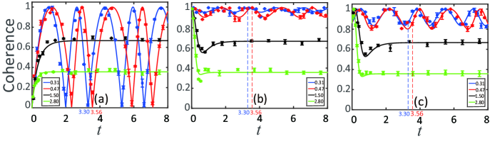
Fig.  2: The evolution of coherence for three initial quantum states in the $\mathcal{PT}$-symmetric system. (a) is for the initial state $|H\rangle$, (b) is for the initial state $(|H\rangle+|V\rangle)/\sqrt{2}$, (c) is for the inital state $(|H\rangle+\sqrt{3}|V\rangle)/2$. In (a, b, c), the periodic oscillation (coherence periodic backflow) happens when $a=0.31$ (blue curve) and $a=0.47$ (red curve) (the $\mathcal{PT}$ symmetry unbroken regime), while the phenomenon of stable value (PSV) of coherence occurs when $a=1.5$ (black curve) and $a=2.8$ (green curve) (the $\mathcal{PT}$ symmetry broken regime). In (a, b, c), $T=3.30$ for $a=0.31$, $T=3.56$ for $a=0.47$. In (a), $SV=0.67$ for $a=1.5$, $SV=0.36$ for $a=2.8$. In (b), $SV=0.67$ for $a=1.5$, $SV=0.36$ for $a=2.8$. In (c), $SV=0.67$ for $a=1.5$, $SV=0.36$ for $a=2.8$. “$SV$” means stable value. All curves are theoretical results while the dots are the experimental data. The experimental errors of one standard deviation (1 SD) are estimated from the statistical variation of photon counts, which satisfy the Poisson distribution.

Experimental results. Figure 2(a, b, c) demonstrate the time-evolution dynamics of the coherence of three initial quantum states $|H\rangle$, $(|H\rangle+|V\rangle)/\sqrt{2}$, and $(|H\rangle+\sqrt{3}|V\rangle)/2$ in the $\mathcal{PT}$-symmetric system. Coherence varies over time $t$ for: (i) $a=0.31$ (blue curve), $a=0.47$ (red curve) $(0<a<1)$; and (ii) $a=1.5$ (blue curve), $a=2.8$ (green curve) $(a>1)$. For $0<a<1$ (the $\mathcal{PT}$ symmetry unbroken regime), coherence oscillates (see blue and red curves) suggesting a coherence complete recovery and backflow. There are two complete backflows of coherence in one period, i.e., double touch of coherence (DTC), which is observed in our experiment and agrees with our theoretical results (see Supplementary Note 3). However, for $a>1$ (the $\mathcal{PT}$ symmetry broken regime), a PSV of coherence occurs (see dark and green curves). Extracted from the experimental data, the recurrence time fits the theoretical value given by

$$T_{\mathcal{PT}}=\frac{\pi}{\sqrt{1-a^{2}}},$$ (11)

and the stable value for the PSV agrees well with the theoretical value $1/a$ (see Supplementary Note 1).

For the same three initial quantum states in the $H_{\mathcal{APT}}$ case, the dynamical characteristics of coherence are shown in Fig. 3, where Figs. 3(a, b, c) are respectively for the initial states $|H\rangle$, $(|H\rangle+|V\rangle)/\sqrt{2}$ and $(|H\rangle+\sqrt{3}|V\rangle)/2$. In contrast to the $H_{\mathcal{PT}}$ case, coherence oscillations occur for $a>1$ (the $\mathcal{APT}$ symmetry unbroken regime), while PSV occurs for $0<a<1$ (the $\mathcal{APT}$ symmetry broken regime), as verified in Figs. 3(a, b, c). Different from the PSV in the $\mathcal{PT}$-symmetric system, the stable value for the PSV in the $\mathcal{APT}$-symmetric system is 1 (see blue and red curves). Figure 3(b) shows that the saturated coherence does not change over time $t$ for any value of $a$. As demonstrated in Figs. 3(a, c), there exits only a single backflow in one period (see dark and green curves), i.e. the DTC phenomenon does not occur in the $\mathcal{APT}$-symmetric system (the theoretical proof is in Supplementary Note 4).

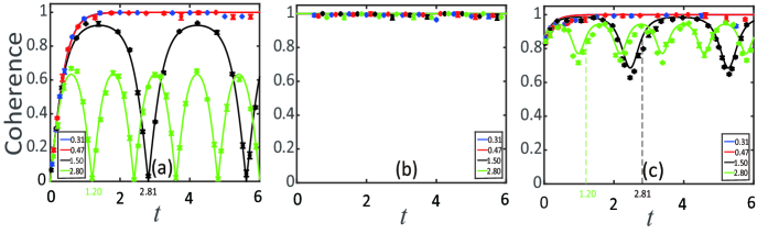
Fig.  3: The evolution of coherence for three initial quantum states in the $\mathcal{APT}$-symmetric system. (a) is for the initial state $|H\rangle$, (b) is for the initial state $(|H\rangle+|V\rangle)/\sqrt{2}$, while (c) is for the initial state $(|H\rangle+\sqrt{3}|V\rangle)/2$. In (a) and (c), the coherence evolution exhibits periodic backflow when $a=1.5$ (black curve) and $a=2.8$ (green curve) (the $\mathcal{APT}$ symmetry unbroken regime), while the PSV of coherence occurs when $a=0.31$ (blue curve) and $a=0.47$ (red curve) (the $\mathcal{APT}$ symmetry broken regime). In (b), coherence is conserved and does not change over time $t$, independent of $a$. In (a) and (c), $T=2.81$ for $a=1.5$, $T=1.20$ for $a=2.8$. All curves are theoretical results while the dots are the experimental data. The experimental errors of 1 SD are estimated from the statistical variation of photon counts, which satisfy the Poisson distribution.

The oscillating period observed in the experiment is consistent with the theoretical value given by

$$T_{\mathcal{APT}}=\frac{\pi}{\sqrt{a^{2}-1}},$$ (12)

and the stable value for the PSV observed in the experiment is in a good agreement with the theoretical value 1 (see Supplementary Note 2).

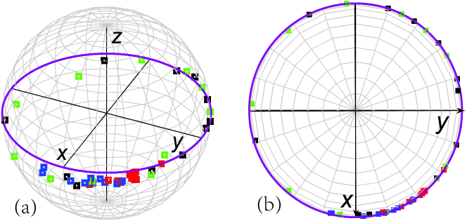
Fig.  4: The trajectory evolution of the initial quantum state $\left(|H\rangle+|V\rangle\right)/\sqrt{2}$ shown by a circle on the Bloch sphere in the $\mathcal{APT}$-symmetric system for different values of $a$. (a) 3D and (b) overhead views. All curves are theoretical results, while squares represent the measured quantum states in our experiment for different evolution times. Different-color squares represent different values of $a$ (blue square: $a=0.31$, red square: $a=0.47$, black square: $a=1.5$, green square: $a=2.8$). Note that the coherences of quantum states on the purple circle are the same. No error bar is plotted because it is difficult to show the error of a quantum state on the Bloch sphere.

To better understand Fig. 3(b), we plot Fig. 4, which shows the trajectory evolution of the initial quantum state $\left(|H\rangle+|V\rangle\right)/\sqrt{2}$ on the Bloch sphere in the $\mathcal{APT}$-symmetric system. Figure 4 shows that the evolved quantum state travels over time along the outer edge of the $XY$ plane, which is independent of $a$. Thus, it can intuitively reflect why the coherence of the quantum state [shown in Fig. 3(b)] remains unchanged during the time evolution.

III Discussion

Our setup provides a simple platform to investigate both $\mathcal{PT}$- and $\mathcal{APT}$-symmetric systems. First, the gain and loss, associated with dissipative coupling between the system and environment, can be readily simulated with optical elements. By selecting the appropriate combination of optical elements with adjustable angles, both $\mathcal{PT}$- and $\mathcal{APT}$-symmetric systems can be realized with this setup. Second, our setup can be used to demonstrate the dynamics of $\mathcal{PT}$- and $\mathcal{APT}$-symmetric systems for each given evolution time $t$, by performing the corresponding nonunitary gate operations on the initial states. The dynamics of $\mathcal{PT}$- and $\mathcal{APT}$-symmetric systems for each given evolution time $t$ is stable and the coherence time of photons is long enough, thus one can accurately extract the critical information from the nonunitary dynamics.

Let us briefly recall the difference between Rabi oscillations and coherence flow oscillations. In our work, we only consider a single qubit, with the usual two logical states $|0\rangle$ and $|1\rangle$. Rabi oscillations refer to the dynamical evolution of the population probability of the logical state $|0\rangle$ or $|1\rangle$ of the qubit. For example, this occurs when the qubit is placed inside a cavity and the cavity-qubit coupling is sufficiently strong, so there is an exchange of energy between the qubit and the photons bouncing back and forth many times inside the cavity. Also, Rabi oscillations occur when a classical driving field is applied to a qubit, where there is an exchange of energy between the qubit and the drive, and the Rabi frequency is proportional to the applied driving field amplitude. On the other hand, for a single qubit, the coherence of quantum states is defined as the sum of the two off-diagonal elements of the single-qubit density matrix, according to Eq. (9). Coherence flow oscillations refer to the oscillations of the coherence of quantum states. Different from Rabi oscillations, coherence flow oscillations do not require the qubit to exchange energy with photons located in a cavity or exchange energy with a classical pulse. Clearly, Rabi oscillations and coherence flow oscillations are completely different notions.

Now let us make a brief comparison with previous works XiaoL2 ; kka ; Chenpx ; Wen , which are most relevant to this work:

(i) A theoretical and experimental research on the dynamics of coherence under $\mathcal{PT}$-symmetric system has been recently presented by Wang et al. Chenpx in a single-ion system. There, the coherence evolution was discussed by the time average of the coherence and the diagonal element (e.g., $\rho_{00}$) of the quantum state density matrix Chenpx . In our work, we provide a simple platform to demonstrate $\mathcal{PT}$- and $\mathcal{APT}$-symmetric systems in experiments. We discuss the $l_{1}$ norm of the coherence (i.e., the summation of off-diagonal elements of the density matrix), which is quite different from the time average of the coherence. Furthermore, we theoretically predict some phenomena (the DTC and PSV phenomena) which were not reported by Wang et al. Chenpx , and give an experimental demonstration in a linear optical system.

(ii) In previous works on information flow kka ; XiaoL2 , the trace distance

$$D\left(\rho_{1}(t),~{}\rho_{2}(t)\right)=\frac{1}{2}\rm Tr|\rho_{1}(t)-\rho_{2}(t)|$$ (13)

was introduced to characterize the information flow; while in our work the $l_{1}$ norm of the coherence, described by Eq. (9), is introduced to characterize the coherence flow. The concept of coherence flow is different from information flow. Second, the trace distance $D\left(\rho_{1}(t),~{}\rho_{2}(t)\right)$ generally measures the distinguishability of two quantum states, while the $l_{1}$ norm of coherence quantifies the coherence of a quantum state. In this sense, the physical meaning of the coherence flow is different from that of the information flow. Third, the physical phenomena revealed by the coherence flow and the information flow are not exactly the same. For example, we found that in the $\mathcal{PT}$-symmetry unbroken regime, there are two complete coherence backflows in one period; while, the previous works kka ; XiaoL2 showed that in the $\mathcal{PT}$-symmetry unbroken regime, there exists only one information flow within one period. Last, quantum coherence is an intriguing property of quantum states, which is a key resource in quantum computing, quantum communication, and quantum metrology; and the $\mathcal{PT}$/$\mathcal{APT}$ systems have attracted considerable interest. Thus, we believe that it is significant to study the evolution of coherence of quantum states in $\mathcal{PT}$ and $\mathcal{APT}$ systems.

(iii) It is obvious that our work differs from the work by Wen et al. Wen . Their work studied the information flow in an $\mathcal{APT}$-symmetry system, which is different from the coherence flow; while, the present work focuses on the coherence flow.

IV Conclusions

In summary, we have experimentally demonstrated the coherence flow in both $\mathcal{PT}$- and $\mathcal{APT}$-symmetric systems by using a single-photon qubit. In this paper, the DTC phenomenon in one period in the $\mathcal{PT}$-symmetric unbroken regime has been demonstrated, which however does not occur in the $\mathcal{APT}$-symmetric system. Moreover, the PSV has been observed in the $\mathcal{PT}$/$\mathcal{APT}$-symmetric broken regime, which is independent of the initial state. As an extension of this work, we have numerically simulated the dynamics of coherence for two-qubit $\mathcal{PT}$/$\mathcal{APT}$ systems (for details, see Supplementary Note 6). The simulations show that for both two-qubit $\mathcal{PT}$/$\mathcal{APT}$ systems, there exist different periodic oscillations of coherence (including one coherence backflow, two coherence backflows, and multiple coherence backflows in one period) in the unbroken regime; while there exists PSV in the broken regime, which is independent of the initial state. Our work merits future study on the multi-qubit coherence flow in $\mathcal{PT}$-and $\mathcal{APT}$-symmetric systems, which is left as an open question.

V Methods

Device parameters. The photon-source system of the single-qubit, the pump laser power is 130 $\rm{mW}$. In the state preparation part, three initial quantum states $|H\rangle$, $\left(|H\rangle+|V\rangle\right)/\sqrt{2}$, and $\left(|H\rangle+\sqrt{3}|V\rangle\right)/2$ corresponding angles of HWP are $0^{\circ}$, $22.5^{\circ}$ and $30^{\circ}$, respectively. In the measure part, the four bases $\left\{|H\rangle,|V\rangle,|R\rangle=\left(|H\rangle-i|V\rangle\right)/\sqrt{2},|D\rangle=\left(|H\rangle+|V\rangle\right)/\sqrt{2}\right\}$ corresponding angles of QWP-HWP are $\left(0^{\circ},0^{\circ}\right)$, $\left(0^{\circ},45^{\circ}\right)$, $\left(0^{\circ},22.5^{\circ}\right)$ and $\left(45^{\circ},22.5^{\circ}\right)$, respectively.

Analysis of experimental imperfections. Due to the accuracy of the rotation angle, and the imperfection of the interference visibility between BDs, several points of experiment data do not fit well with our theoritical data. To solve this problem, we improve the extinction ratio of interference between BDs for a high interference visibility. Instead of manual adjustment, we use motorized precision rotation mount to ensure the higher accuracy of the plate rotation angle. Meanwhile, the experimental errors are estimated from the statistical variation of photon counts, which satisfy the Poisson distribution.

Data availability

The data that support the findings of this study are available from the corresponding authors upon reasonable request.

Code availability

The code used for simulations is available from the corresponding authors upon reasonable request.

Author contributions

Y.-L. F. performed the experiment and analyzed the data with the assistance of Y.Z., J.-L.Z and C.-P. Y., Y.Z. proposed the experiment and designed experimental scheme. J.-L. Z. provided the theoretical analytic proofs of our results. C.-P. Y. and F. N. directed the project. J.-L. Z, Y. Z. D.-X. C Y.-H. Z., Q.-C. W. C.-P Y. and F. N. provided theoretical support. Y.Z., J.-L.Z., Q.-C.W., C.-P.Y., and N.F. wrote the manuscript with feedback from all authors.

Competing interests

The authors declare no competing interests

References

Bender, C. M. & Boettcher, S. Real Spectra in Non-Hermitian Hamiltonians Having PT Symmetry. Phys. Rev. Lett. 80, 5243-5246 (1998).

Konotop, V. V., Yang, J. & Zezyulin, D. A. Nonlinear waves in PT-symmetric systems. Rev. Mod. Phys. 88, 035002 (2016).

El-Ganainy, R., Makris, K. G., Khajavikhan, M., Musslimani, Z. H., Rotter, S. & Christodoulides, D. N. Non-Hermitian physics and PT symmetry. Nat. Phys. 14, 11-19 (2018).

Schindler, J., Li, A., Zheng, M. C., Ellis, F. M. & Kottos, T. Experimental study of active LRC circuits with PT symmetries. Phys. Rev. A 84, 040101 (2011).

Abdullaev, F. K., Kartashov, Y. V., Konotop, V. V. & Zezyulin, D. A. Solitons in PT-symmetric nonlinear lattices. Phys. Rev. A 83, 041805 (2011).

Chong, Y. D., Ge, L. & Stone, A. D. PT-Symmetry Breaking and Laser-Absorber Modes in Optical Scattering Systems. Phys. Rev. Lett. 106, 093902 (2011).

Regensburger, A., Bersch, C., Miri, M. A., Onishchukov, G., Christodoulides, D. N. & Peschel, U. Parity-time synthetic photonic lattices. Nature 488, 167-171 (2012).

Feng, L., Xu, Y. L., Fegadolli, W. S., Lu, M. H., Oliveira, J. E. B., Almeida, V. R., Chen, Y. F. & Scherer, A. Experimental demonstration of a unidirectional reflection less parity-time metamaterial at optical frequencies. Nat. Mater. 12, 108-113 (2013).

Peng, B., Özdemir, S. K., Rotter, S., Yilmaz, H., Liertzer, M., Monifi, F., Bender, C. M., Nori, F. & Yang, L. Loss-induced suppression and revival of lasing. Science 346, 328-332 (2014).

Jing, H., Özdemir, S. K., Lu, X. Y., Zhang, J., Yang, L. & Nori, F. PT-Symmetric Phonon Laser. Phys. Rev. Lett. 113, 053604 (2014).

Lee, Y. C., Hsieh, M. H., Flammia, S. T. & Lee, R. K. Local PT symmetry violates the no-signaling principle. Phys. Rev. Lett. 112, 130404 (2014).

Peng, B., Özdemir, S. K., Lei, F., Monifi, F., Gianfreda, M., Long, G. L., Fan, S., Nori, F., Bender, C. M. & Yang, L. Parity-time-symmetric whispering-gallery microcavities. Nat. Phys. 10, 394-398 (2014).

Ju, C. Y. et al., Non-Hermitian Hamiltonians and no-go theorems in quantum information. Phys. Rev. A 100, 062118 (2019).

Arkhipov, I. I. et al., Scully-Lamb quantum laser model for parity-time-symmetric whispering-gallery microcavities: Gain saturation effects and nonreciprocity. Phys. Rev. A 99, 053806 (2019).

Song, Q. J., Hu, J. S., Dai, S. W., Zheng, C. X., Han, D. Z., Zi, J., Zhang, Z. Q. & Chan, C. T. Coexistence of a new type of bound state in the continuum and a lasing threshold mode induced by PT symmetry. Sci. Adv. 6, 1160 (2020).

Hang, C., Huang, G. X. & Konotop, V. V. PT symmetry with a system of three-level atoms. Phys. Rev. Lett. 110, 083604 (2013).

Tang, J. S., Wang, Y. T., Yu, S., He, D. Y., Xu, J. S., Liu, B. H., Chen, G., Sun, Y. N., Sun, K., Han, Y. J., Li, C. F. & Guo, G. C. Experimental investigation of the no-signalling principle in parity-time symmetric theory using an open quantum system. Nat. Photonics 10, 642-646 (2016).

Kawabata, K., Ashida, Y. & Ueda, M. Information retrieval and criticality in parity-time-symmetric systems. Phys. Rev. Lett. 119, 190401 (2017).

Zhang, J., Peng, B., Özdemir, S. K., Pichler, K., Krimer, D. O., Zhao, G., Nori, F., Liu, Y. X, Rotter, S. & Yang, L. A phonon laser operating at an exceptional point. Nat. Photonics 12, 479-484 (2018).

Quijandria, F., Naether, U., Özdemir, S. K., Nori, F. & Zueco, D. PT-symmetric circuit QED. Phys. Rev. A 97, 053846 (2018).

Özdemir, S. K., Rotter, S., Nori, F. & Yang, L. Parity-time symmetry and exceptional points in photonics. Nat. Mater. 18, 783-789 (2019).

Li, J., Harter, A. K., Liu, J., de Melo, L., Joglekar, Y. N. & Luo, L. Observation of parity-time symmetry breaking transitions in a dissipative Floquet system of ultracold atoms. Nat. Commun. 10, 855 (2019).

Xiao, L., Wang, K. K., Zhan, X., Bian, Z. H., Kawabata, K., Ueda, M., Yi, W. & Xue, P. Observation of Critical Phenomena in Parity-Time-Symmetric Quantum Dynamics. Phys. Rev. Lett. 123, 230401 (2019).

Wang, Y. T., Li, Z. P., Yu, S., Ke, Z. J., Liu, W., Meng, Y., Yang, Y. Z., Tang, J. S., Li, C. F. & Guo, G. C. Experimental Investigation of State Distinguishability in Parity-Time Symmetric Quantum Dynamics. Phys. Rev. Lett. 124, 230402 (2020).

Bian, Z. H., Xiao, L., Wang, K. K., Zhan, X., Onanga, F. A., Ruzicka, F., Yi, W., Joglekar, Y. N. & Xue, P. Conserved quantities in parity-time symmetric systems. Phys. Rev. Research 2, 022039 (2020).

Arkhipov, I. I. et al., Liouvillian exceptional points of any order in dissipative linear bosonic systems: Coherence functions and switching between PT and anti-PT symmetries. Phys. Rev. A 102, 033715 (2020).

Feng, L., Wong, Z. J., Ma, R.-M., Wang, Y. & Zhang, X. Single-mode laser by parity-time symmetry breaking. Science 346, 972-975 (2014).

Hodaei, H., Miri, M. A., Heinrich, M., Christodoulides, D. N. & Khajavikhan, M. Parity-Time-symmetric microring lasers. Science 346, 975-978 (2014).

Smirnov, S. V., Makarenko, M. O., Suchkov, S. V., Churkin, D. & Sukhorukov, A. A. Bistable lasing in parity-time symmetric coupled fiber rings. Photonics Res. 6, A18-A22 (2018).

Guo, A., Salamo, G. J., Duchesne, D., Morandotti, R., Volatier-Ravat, M., Aimez, V., Siviloglou, G. A. & Christodoulides, D. N. Observation of PT Symmetry Breaking in Complex Optical Potentials. Phys. Rev. Lett. 103, 093902 (2009).

Liu, Z. P. et al., Metrology with PT-Symmetric Cavities: Enhanced Sensitivity near the PT-Phase Transition. Phys. Rev. Lett. 117, 110802 (2016).

Chen, W., Özdemir, S. K., Zhao, G., Wiersig, J. & Yang, L. Exceptional points enhance sensing in an optical microcavity. Nature 548, 192-196 (2017).

Hodaei, H., Hassan, A. U., Wittek, S., Garcia-Gracia, H., El-Ganainy, R., Christodoulides, D. N. & Khajavikhan, M. Enhanced sensitivity at higher-order exceptional points. Nature 548, 187-191 (2017).

Rüter, C. E., Makris, K. G., El-Ganainy, R., Christodoulides, D. N., Segev, M. & Kip, D. Observation of parity-time symmetry in optics. Nat. Phys. 6, 192-195 (2010).

Wu, Y., Liu, W. Q., Geng, J. P., Song, X. R., Ye, X. Y., Duan, C. K., Rong, X. & Du, J. F. Observation of parity-time symmetry breaking in a single-spin system. Science 364, 878-880 (2019).

Naghiloo, M., Abbasi, M., Joglekar, Y. N. & Murch, K. W. Quantum state tomography across the exceptional point in a single dissipative qubit. Nat. Phys. 15, 1232-1236 (2019).

Wang, W. C. et al., Observation of PT -symmetric quantum coherence in a single-ion system. Phys. Rev. A 103, L020201 (2021).

Wen, J. W, Zheng, C., Kong, X. Y., Wei, S. J., Xin, T. & Long, G. L. Experimental demonstration of a digital quantum simulation of a general PT -symmetric system. Phys. Rev. A 99, 062122 (2019).

Wen, J. W, Zheng, C., Ye, Z. D., Xin, T. & Long, G. L. Stable states with nonzero entropy under broken PT symmetry. Phys. Rev. Research 3, 013256 (2021).

Ge, L. & Türeci, H. E. Antisymmetric PT photonic structures with balanced positive-and negative-index materials. Phys. Rev. A 88, 053810 (2013).

Knotop, V. V. & Zezyulin, D. A. Odd-Time Reversal PT Symmetry Induced by an Anti-PT-Symmetric Medium. Phys. Rev. Lett. 120, 123902 (2018).

Yang, F., Liu, Y. C. & You, L. Anti-PT symmetry in dissipatively coupled optical systems. Phys. Rev. A 96, 053845 (2017).

Li, Q. et al., Experimental simulation of anti-parity-time symmetric Lorentz dynamics. Optica 6, 67-71 (2019).

Wu, J. H., Artoni, M. & La Rocca, G. C. Parity-time-antisymmetric atomic lattices without gain. Phys. Rev. A 91, 033811 (2015).

Peng, P., Cao, W. X., Shen, C., Qu, W. Z., Wen, J. M., Jiang, L. & Xiao, Y. H. Anti-parity-time symmetry with flying atoms. Nat. Phys. 12, 1139-1145 (2016).

Chuang, Y.L., Ziauddin & Lee, R. K. Realization of simultaneously parity-time-symmetric and parity-time-antisymmetric susceptibilities along the longitudinal direction in atomic systems with all optical controls. Opt. Express 26, 21969-21978 (2018).

Jiang, Y., Mei, Y. F., Zuo, Y., Zhai, Y. H., Li, J. S., Wen, J. M. & Du, S. W. Anti-Parity-Time Symmetric Optical Four-Wave Mixing in Cold Atoms. Phys. Rev. Lett. 123, 193604 (2019).

Choi, Y., Hahn, C., Yoon, J. W. & Song, S. H. Observation of an anti-PT -symmetric exceptional point and energy-difference conserving dynamics in electrical circuit resonators. Nat. Commun. 9, 2182 (2018).

Zhao, J., Liu, Y. L., Wu, L. H., Duan, C. K., Liu, Y. X. & Du, J. F. Observation of Anti-PT-Symmetry Phase Transition in the Magnon-Cavity-Magnon Coupled System. Phys. Rev. Appl. 13, 014053 (2020).

Li, Y. et al., Anti-parity-time symmetry in diffusive systems. Science 364, 170-173 (2019).

Zhang, H. L. et al., Breaking Anti-PT Symmetry by Spinning a Resonator. Nano Letters 20, 7594 (2020).

Wen, J. W., Qin, G. Q., Zheng, C., Wei, S. J., Kong, X. Y., Xin, T. & Long, G. L. Observation of information flow in the anti-PT symmetric system with nuclear spins. npj Quantum Inf. 6, 28 (2020).

Stewart, G. W. Computing the CS decomposition of a partitioned orthonormal matrix. Numer. Math. 40, 297-306 (1982).

Brody, D. C. & Graefe, E. M. Mixed-State Evolution in the Presence of Gain and Loss. Phys. Rev. Lett. 109, 230405 (2012).

Baumgratz, T., Cramer, M. & Plenio, M. B. Quantifying coherence. Phys. Rev. Lett. 113,140401(2014).

Mani, A. & Karimipour, V. Cohering and decohering power of quantum channels. Phys. Rev. A 92, 032331(2015).

Supplementary Information for:
Experimental demonstration of coherence flow in $\mathcal{PT}$- and anti-$\mathcal{PT}$-symmetric systems

VI Phenomenon of stable value and the period of coherent evolution in $\mathcal{PT}$-symmetric systems

Let us first consider the $\mathcal{PT}$-symmetric non-Hermitian Hamiltonian shown in Eq. (1) of the main text. The evolution of quantum states in $\mathcal{PT}$-symmetric systems is described by the time-evolution operator $U_{\mathcal{PT}}=\exp(-i\hat{H}_{\mathcal{PT}}t)$:

$$\boldsymbol{U}_{\mathcal{PT}}(t) = \exp(-\emph{i}\hat{H}_{\mathcal{PT}}t)$$ (S3)

$$= \exp\left[-\emph{i}s(\sigma_{x}+\emph{i}a\sigma_{z})t\right]$$

$$= \exp\left[s\left(\begin{array}[]{cc}a&-\emph{i}\\ -\emph{i}&-a\end{array}\right)t\right]$$

$$= \left(\begin{array}[]{cc}A-B&-\emph{i}C\\ -\emph{i}C&A+B\end{array}\right).$$ (S6)

Here $A$, $B$ and $C$ are given by:

(i) for $0<a<1$,

$$A=\cos\left(\omega_{1}st\right),~{}~{}B=-\frac{a}{\omega_{1}}\sin\left(\omega_{1}st\right),~{}~{}C=\frac{1}{\omega_{1}}\sin\left(\omega_{1}st\right),$$ (S7)

where $\omega_{1}=\sqrt{1-a^{2}}>0$.

(ii) for $a>1$,

$$A=\cosh\left(\omega_{2}st\right),~{}~{}B=-\frac{a}{\omega_{2}}\sinh\left(\omega_{2}st\right),~{}~{}C=\frac{1}{\omega_{2}}\sinh\left(\omega_{2}st\right),$$ (S8)

where $\omega_{2}=\sqrt{a^{2}-1}>0$.

In general, the initial state is $|\phi\rangle=\alpha|H\rangle+\beta e^{i\varphi}|V\rangle$, where $\alpha,\beta\in\left[0,1\right]$, $\alpha^{2}+\beta^{2}=1$ and $\varphi\in\left[0,2\pi\right]$. The time-evolved state is expressed as:

$$|\phi(t)\rangle = \frac{\boldsymbol{U}_{\mathcal{PT}}|\phi\rangle}{\|\boldsymbol{U}_{\mathcal{PT}}|\phi\rangle\|}$$ (S11)

$$= \frac{1}{\sqrt{M}}\left(\begin{array}[]{c}\alpha(A-B)-iC\beta e^{i\varphi}\\ (A+B)\beta e^{i\varphi}-iC\alpha\end{array}\right),$$

where $\||\cdot\rangle\|=\sqrt{\operatorname{Tr}\left(|\cdot\rangle\langle\cdot|\right)}$ denotes the normalization coefficient, and

$$M=\||\cdot\rangle\|^{2}=A^{2}+B^{2}+C^{2}+2AB\left(\beta^{2}-\alpha^{2}\right)-4\alpha\beta BC\sin\varphi.$$ (S12)

Thus, the coherence of the state $|\phi(t)\rangle$ is given by:

$$C_{l_{1}}\left(|\phi(t)\rangle\right)=\frac{2\left\{\left[\alpha^{2}(A-B)^{2}+C^{2}\beta^{2}+2\alpha\beta(AC-BC)\sin\varphi\right]\left[C^{2}\alpha^{2}+(A+B)^{2}\beta^{2}-2\alpha\beta(AC+BC)\sin\varphi\right]\right\}^{1/2}}{A^{2}+B^{2}+C^{2}+2AB\left(\beta^{2}-\alpha^{2}\right)-4\alpha\beta BC\sin\varphi}.$$ (S13)

Let us first consider the case when $0<a<1$ (i.e., the $\mathcal{PT}$-symmetric-unbroken regime). In this case, $A$, $B$, and $C$ are given by Eq. (S7). After inserting Eq. (S7) into Eq. (S13), a simple calculation gives:

$$C_{l_{1}}\left(|\phi(t)\rangle\right)=\frac{2\sqrt{m_{1}}}{1+m_{1}},$$ (S14)

where $m_{1}=x_{1}/y_{1}$, with $x_{1}$ and $y_{1}$ given below:

$$x_{1}=\frac{1}{\omega_{1}^{2}}\left[\alpha^{2}\left(\omega_{1}^{2}\cos 2\theta_{1}+a\omega_{1}\sin 2\theta_{1}\right)+\frac{1-\cos 2\theta_{1}}{2}+\alpha\beta\sin\varphi\left(\omega_{1}\sin 2\theta_{1}+a(1-\cos 2\theta_{1})\right)\right],$$

$$y_{1}=\frac{1}{\omega_{1}^{2}}\left[\beta^{2}\left(\omega_{1}^{2}\cos 2\theta_{1}-a\omega_{1}\sin 2\theta_{1}\right)+\frac{1-\cos 2\theta_{1}}{2}-\alpha\beta\sin\varphi\left(\omega_{1}\sin 2\theta_{1}-a(1-\cos 2\theta_{1})\right)\right].$$ (S15)

Here $\theta_{1}=\omega_{1}st$. From Eq. (S14) and Eq. (S15), one can see that $C_{l_{1}}\left(|\phi(t)\rangle\right)$ is a function of $\sin 2\theta_{1}$ and $\cos 2\theta_{1}$. Thus, the period of $C_{l_{1}}\left(|\phi\rangle\right)$ is the same as that of $\sin 2\theta_{1}$ or $\cos 2\theta_{1}$. Note that $\sin 2\theta_{1}$ ($\cos 2\theta_{1}$) can be written as $\sin 2\omega_{1}st$ ($\cos 2\omega_{1}st$) with $\omega_{1}=\sqrt{1-a^{2}}$. Therefore, the period of coherent evolution in $\mathcal{PT}$-symmetric systems is:

$$T_{\mathcal{PT}}=\frac{2\pi}{2\omega_{1}s}=\frac{\pi}{s\sqrt{1-a^{2}}}.$$ (S16)

Now, let us consider the case $a>1$ (i.e., the $\mathcal{PT}$-symmetric-broken regime). In this situation, $A$, $B$, and $C$ are given by Eq. (S8). Substitution of Eq. (S8) into Eq. (S13) gives:

$$C_{l_{1}}\left(|\phi(t)\rangle\right)=\frac{2\sqrt{m_{2}}}{1+m_{2}},$$ (S17)

where $m_{2}=x_{2}/y_{2}$, with $x_{2}$ and $y_{2}$ given by

$$x_{2}=\alpha^{2}\left(\cosh\theta_{2}+\frac{a}{\omega_{2}}\sinh\theta_{2}\right)^{2}+\frac{1}{\omega_{2}^{2}}\beta^{2}\sinh^{2}\theta_{2}+2\alpha\beta\left(\frac{1}{\omega_{2}}\cosh\theta_{2}\sinh\theta_{2}+\frac{a}{\omega_{2}}\sinh^{2}\theta_{2}\right)\sin\varphi,$$

$$y_{2}=\beta^{2}\left(\cosh\theta_{2}-\frac{a}{\omega_{2}}\sinh\theta_{2}\right)^{2}+\frac{1}{\omega_{2}^{2}}\alpha^{2}\sinh^{2}\theta_{2}-2\alpha\beta\left(\frac{1}{\omega_{2}}\cosh\theta_{2}\sinh\theta_{2}-\frac{a}{\omega_{2}^{2}}\sinh^{2}\theta_{2}\right)\sin\varphi.$$ (S18)

Here $\theta_{2}=\omega_{2}st$. When $t\rightarrow\infty$, $\cosh\theta_{2}\thicksim\sinh\theta_{2}\rightarrow\infty$. Thus, it is straightfordward to find from Eqs. (S17) and (S18) that:

$$\lim_{t\rightarrow\infty}C_{l_{1}}\left(|\phi(t)\rangle\right) = \frac{2\left\{a^{2}+\omega_{2}^{2}(\alpha^{2}-\beta^{2})^{2}+2a\omega_{2}(\alpha^{2}-\beta^{2})+4\alpha\beta\sin\varphi\left[a+\omega_{2}(\alpha^{2}-\beta^{2})\right]+4\alpha^{2}\beta^{2}\sin^{2}\varphi\right\}^{1/2}}{2a^{2}+2a\omega_{2}\left(\alpha^{2}-\beta^{2}\right)+4a\alpha\beta\sin\varphi}$$ (S19)

$$= \frac{2\left[a+\omega_{2}(\alpha^{2}-\beta^{2})+2\alpha\beta\sin\varphi\right]}{2a^{2}+2a\omega_{2}\left(\alpha^{2}-\beta^{2}\right)+4a\alpha\beta\sin\varphi}$$

$$= \frac{1}{a}.$$

Equation (S19) shows that the phenomenon of stable value (PSV) of coherence occurs after a long time evolution; that is, the coherence tends to a stable value $1/a$, which is independent of the initial states.

VII Phenomenon of stable value and the period of coherent evolution in anti-$\mathcal{PT}$-symmetric systems

Let us now consider the anti-$\mathcal{PT}$($\mathcal{APT}$)-symmetric non-Hermitian Hamiltonian in Eq. (2) of the main text. The evolution of the quantum states in $\mathcal{APT}$-symmetric systems is governed by the operator $U_{\mathcal{APT}}=\exp(-i\hat{H}_{\mathcal{APT}}t)$:

$$\boldsymbol{U}_{\mathcal{APT}}(t) = \exp(-i\hat{H}_{\mathcal{APT}}t)$$ (S22)

$$= \exp\left[-is(i\sigma_{x}+a\sigma_{z})t\right]$$

$$= \exp\left[s\left(\begin{array}[]{cc}-ia&1\\ 1&ia\end{array}\right)t\right]$$

$$= \left(\begin{array}[]{cc}A+iB&C\\ C&A-iB\end{array}\right).$$ (S25)

Here $A$, $B$ and $C$ are given by:

(i) for $a>1$,

$$A=\cos\left(\omega_{3}st\right),~{}~{}B=-\frac{a}{\omega_{3}}\sin\left(\omega_{3}st\right)t,~{}~{}C=\frac{1}{\omega_{3}}\sin\left(\omega_{3}st\right),$$ (S26)

where $\omega_{3}=\sqrt{a^{2}-1}>0$.

(ii) for $0<a<1$,

$$A=\cosh\left(\omega_{4}st\right),~{}~{}B=-\frac{a}{\omega_{4}}\sinh\left(\omega_{4}st\right),~{}~{}C=\frac{1}{\omega_{4}}\sinh\left(\omega_{4}st\right),$$ (S27)

where $\omega_{4}=\sqrt{1-a^{2}}>0$.

In general, the initial state is $|\phi\rangle=\alpha|H\rangle+\beta e^{i\varphi}|V\rangle$. The time-evolved state is given by:

$$|\phi(t)\rangle = \frac{\boldsymbol{U}_{\mathcal{APT}}|\phi\rangle}{\|\boldsymbol{U}_{\mathcal{APT}}|\phi\rangle\rangle\|}$$ (S30)

$$= \frac{1}{\sqrt{M}}\left(\begin{array}[]{c}\alpha(A+Bi)+C\beta e^{i\varphi}\\ (A-Bi)\beta e^{i\varphi}+C\alpha\end{array}\right),$$

where $M=A^{2}+B^{2}+C^{2}+4C\left(A\cos\varphi+B\sin\varphi\right)\alpha\beta$. The coherence of $|\phi(t)\rangle$ is:

$$C_{l_{1}}\left(|\phi(t)\rangle\right)=\frac{2\left\{\left[(A\alpha+C\beta\cos\varphi)^{2}+(B\alpha+C\beta\sin\varphi)^{2}\right]\left[\left((A\cos\varphi+B\sin\varphi)\beta+C\alpha\right)^{2}+(A\sin\varphi-B\cos\varphi)^{2}\beta^{2}\right]\right\}^{1/2}}{A^{2}+B^{2}+C^{2}+4C\left(A\cos\varphi+B\sin\varphi\right)\alpha\beta}.$$ (S31)

Let us first consider the case $a>1$ (i.e., the $\mathcal{APT}$-symmetric-unbroken regime). In this case, $A$, $B$ and $C$ are given by Eq. (S26). After inserting Eq. (S26) into Eq. (S31), we obtain:

$$C_{l_{1}}\left(|\phi(t)\rangle\right)=\frac{2\sqrt{m_{3}}}{1+m_{3}},$$ (S32)

where $m_{3}=x_{3}/y_{3}$, with $x_{3}$ and $y_{3}$ given below:

$$x_{3}=\frac{1}{\omega_{3}^{2}}\left[\omega_{3}^{2}\alpha^{2}+\alpha\beta\omega_{3}\cos\varphi\sin 2\theta_{3}+\frac{1-\cos 2\theta_{3}}{2}\left(1-a\alpha\beta\sin\varphi\right)\right],$$

$$y_{3}=\frac{1}{\omega_{3}^{2}}\left[\omega_{3}^{2}\beta^{2}+\alpha\beta\omega_{3}\cos\varphi\sin 2\theta_{3}+\frac{1-\cos 2\theta_{3}}{2}\left(1-a\alpha\beta\sin\varphi\right)\right].$$ (S33)

Here $\theta_{3}=\omega_{3}st$. Based on Eq. (S32) and Eq. (S33), one sees that $C_{l_{1}}\left(|\phi(t)\rangle\right)$ is a function of $\sin 2\theta_{3}$ and $\cos 2\theta_{3}$; that is, $\sin 2\omega_{3}st$ and $\cos 2\omega_{3}st$. Hence, the period of coherent evolution in $\mathcal{APT}$-symmetric systems is:

$$T_{\mathcal{APT}}=\frac{2\pi}{2\omega_{3}s}=\frac{\pi}{s\sqrt{a^{2}-1}}.$$ (S34)

Let us now consider the case of $0<a<1$ (i.e., the $\mathcal{APT}$-symmetric-broken regime). In this situation, $A$, $B$ and $C$ are given by Eq. (S27). Substitution of Eq. (S27) into Eq. (S31) leads to:

$$C_{l_{1}}\left(|\phi(t)\rangle\right)=\frac{2\sqrt{m_{4}}}{1+m_{4}},$$ (S35)

where $m_{4}=x_{4}/y_{4}$, with $x_{4}$ and $y_{4}$ given below:

$$x_{4}=\frac{1}{\omega_{4}^{2}}\left[\left(\omega_{4}^{2}\cosh^{2}\theta_{4}+a^{2}\sinh^{2}\theta_{4}\right)\alpha^{2}+\beta^{2}\sinh^{2}\theta_{4}+2\alpha\beta\sinh\theta_{4}\left(\omega_{4}\cos\varphi\cosh\theta_{4}-a\sinh\theta_{4}\sin\varphi\right)\right],$$

$$y_{4}=\frac{1}{\omega_{4}^{2}}\left[\left(\omega_{4}^{2}\cosh^{2}\theta_{4}+a^{2}\sinh^{2}\theta_{4}\right)\beta^{2}+\alpha^{2}\sinh^{2}\theta_{4}+2\alpha\beta\sinh\theta_{4}\left(\omega_{4}\cos\varphi\cosh\theta_{4}-a\sinh\theta_{4}\sin\varphi\right)\right].$$ (S36)

Here $\theta_{4}=\omega_{4}st$. When $t\rightarrow\infty$, $\cosh\theta_{4}\thicksim\sinh\theta_{4}\rightarrow\infty$. Thus, it follows from Eq. (S36) that:

$$x_{4}\thicksim y_{4}\thicksim\frac{1+2\alpha\beta(\sqrt{1-a^{2}}\cos\varphi-a\sin\varphi)}{1-a^{2}}\sinh^{2}\theta_{4}.$$ (S37)

Accordingly, it follows from Eq. (S35) that:

$$\lim_{t\rightarrow\infty}C_{l_{1}}\left(|\phi(t)\rangle\right) = \lim_{t\rightarrow\infty}\frac{2\sqrt{x_{4}/y_{4}}}{1+x_{4}/y_{4}}$$ (S38)

$$= 1.$$

Equation (S38) shows that the phenomenon of stable value (PSV) of coherence occurs after a long time evolution; that is, the coherence tends to $1$, which is independent of the initial states.

VIII Proof for the characteristics of each backflow in the $\mathcal{PT}$-symmetric-unbroken regime

For an arbitrary initial state $|\phi\rangle=\alpha|H\rangle+\beta e^{i\varphi}|V\rangle$, the coherence of the evolved state $|\phi(t)\rangle$ in the $\mathcal{PT}$-symmetric unbroken regime is given by Eq. (S14). According to Eq. (S14), the derivative of $C_{l_{1}}\left(|\phi(t)\rangle\right)$ can be decomposed into

$$\frac{dC_{l_{1}}\left(|\phi(t)\rangle\right)}{dt}=\frac{dC_{l_{1}}\left(|\phi(t)\rangle\right)}{dm_{1}}\times\frac{dm_{1}}{d\theta_{1}}\times\frac{d\theta_{1}}{dt}.$$ (S39)

Because of $\frac{d\theta_{1}}{dt}=\omega_{1}s>0$, the condition for $\frac{dC_{l_{1}}\left(|\phi(t)\rangle\right)}{dt}=0$ turns into:

$$\frac{dC_{l_{1}}\left(|\phi(t)\rangle\right)}{dm_{1}}=0$$ (S40)

or

$$\frac{dm_{1}}{d\theta_{1}}=0.$$ (S41)

First, we consider the case of $\frac{dC_{l_{1}}\left(|\phi(t)\rangle\right)}{dm}=0$. According to Eq. (S14), we have

$$\frac{dC_{l_{1}}\left(|\phi(t)\rangle\right)}{dm_{1}}=\frac{1-m_{1}}{(1+m_{1})^{2}\sqrt{m_{1}}}=0.$$ (S42)

Because of $m_{1}=x_{1}/y_{1}$, it follows from Eq. (S15) that:

$$m_{1}=\frac{\alpha^{2}\left(\omega_{1}^{2}\cos 2\theta_{1}+a\omega_{1}\sin 2\theta_{1}\right)+\frac{1-\cos 2\theta_{1}}{2}+\alpha\beta\sin\varphi\left[\omega_{1}\sin 2\theta_{1}+a(1-\cos 2\theta_{1})\right]}{\beta^{2}\left(\omega_{1}^{2}\cos 2\theta_{1}-a\omega_{1}\sin 2\theta_{1}\right)+\frac{1-\cos 2\theta_{1}}{2}-\alpha\beta\sin\varphi\left[\omega_{1}\sin 2\theta_{1}-a(1-\cos 2\theta_{1})\right]}.$$ (S43)

After inserting Eq. (S43) into Eq. (S42), we obtain

$$\tan 2\theta_{1}=-\frac{\left(\alpha^{2}-\beta^{2}\right)\omega_{1}}{a+2\alpha\beta\sin\varphi}.$$ (S44)

Note that the period of $\tan 2\theta_{1}$ is $\frac{\pi}{2}$ with respect to $\theta_{1}$, while the period of $C_{l_{1}}\left(|\phi(t)\rangle\right)$ is $T_{\mathcal{PT}}$=$\pi/(\omega_{1}s)$ with respect to $t$. Because of $\theta_{1}$=$\omega_{1}st$, the period $T_{\mathcal{PT}}$=$\pi/(\omega_{1}s)$ can be expressed as $T_{\theta_{1}}$=$\pi$ with respect to $\theta_{1}$. Thus, one period of $C_{l_{1}}\left(|\phi(t)\rangle\right)$ includes two periods of $\tan 2\theta_{1}$; that is, there are two different values of $\theta_{1}$ (or $t$) satisfying Eq. (S44) or Eq. (S40) within one period of $C_{l_{1}}\left(|\phi(t)\rangle\right)$.

Now, we consider the case of $\frac{dm_{1}}{d\theta_{1}}=0$. Based on $m_{1}=x_{1}/y_{1}$, one has

$$\frac{dm_{1}}{d\theta_{1}}=\frac{x_{1}^{\prime}y_{1}-x_{1}y_{1}^{\prime}}{y_{1}^{2}},$$ (S45)

where $x_{1}^{\prime}=\frac{dx_{1}}{d\theta_{1}}$ and $y_{1}^{\prime}=\frac{dy_{1}}{d\theta_{1}}$. It follows from Eq. (S15) that:

$$x_{1}^{\prime}=\frac{1}{\omega_{1}^{2}}\left[\alpha^{2}\left(-2\omega_{1}^{2}\sin 2\theta_{1}+2a\omega_{1}\cos 2\theta_{1}\right)+\sin 2\theta_{1}+\alpha\beta\sin\varphi\left(2\omega_{1}\cos 2\theta_{1}+2a\sin 2\theta_{1}\right)\right],$$

$$y_{1}^{\prime}=\frac{1}{\omega_{1}^{2}}\left[\beta^{2}\left(-2\omega_{1}^{2}\sin 2\theta_{1}-2a\omega_{1}\cos 2\theta_{1}\right)+\sin 2\theta_{1}-\alpha\beta\sin\varphi\left(2\omega_{1}\cos 2\theta_{1}-2a\sin 2\theta_{1})\right)\right].$$ (S46)

Substituting Eq. (S15) and Eq. (S46) into Eq. (S45), one can easily find that the condition for $dm_{1}/d\theta_{1}=0$ is:

$$\left[2a\omega_{1}^{2}\alpha^{2}\beta^{2}-a(4\alpha^{2}\beta^{2}\sin^{2}\varphi+1)-\alpha\beta\sin\varphi(3a^{2}+1)\right]\tan^{2}\theta_{1}-\omega_{1}(1-2\beta^{2})(1-2a\alpha\beta\sin\varphi)\tan\theta_{1}$$

$$+2a\omega_{1}\alpha^{2}\beta^{2}+\alpha\beta\sin\varphi=0.$$ (S47)

Thus, the discriminant of Eq. (S47) is given by:

$$\Delta=g+4(p+q)r,$$ (S48)

with

$$g=\omega_{1}^{2}(\alpha^{2}-\beta^{2})^{2}(1-2a\alpha\beta\sin\varphi)^{2},$$

$$p=4a\alpha^{2}\beta^{2}\sin^{2}\varphi+\alpha\beta\sin\varphi(3a^{2}+1),$$

$$q=a\left[(\alpha^{2}-\beta^{2})^{2}+2(1+a^{2})\alpha^{2}\beta^{2}\right],$$

$$r=2a\omega_{1}^{2}\alpha^{2}\beta^{2}+\alpha\beta\sin\varphi.$$ (S49)

Here, $g\geq 0$ and $q>0$. Without loss of generality, we consider $\sin\varphi\geq 0$ and $\alpha,\beta\in\left(0,~{}1\right)$. In this case, $p\geq 0$ and $r>0$. Hence, we have $\Delta>0$, which implies that $\tan\theta_{1}$ has two different values to satisfy either Eq. (S47) or Eq. (S41). As mentioned above, the period $T_{\mathcal{PT}}$=$\frac{\pi}{s\sqrt{1-a^{2}}}$ of $C_{l_{1}}\left(|\phi(t)\rangle\right)$ can be expressed as $T_{\theta_{1}}$=$\pi$ with respect to $\theta_{1}$. Note that the period of $\tan\theta_{1}$ and the period of $C_{l_{1}}\left(|\phi(t)\rangle\right)$ are $\pi$ with respect to $\theta_{1}$, and $\tan\theta_{1}$ has two different values to satisfy Eq. (S41). Thus, there exist two different values $\theta_{1}$ (or $t$) to satisfy Eq. (S41) within one period of $C_{l_{1}}\left(|\phi(t)\rangle\right)$.

From the above discussion, one can conclude that for a wide rangle of initial states $\alpha|H\rangle+\beta e^{i\varphi}|V\rangle$, with $\alpha,\beta\in\left(0,~{}1\right)$ and $\sin\varphi\geq 0$, the $\frac{dC_{l_{1}}\left(|\phi(t)\rangle\right)}{dt}$ has four zero points in one period (i.e., $T$=$\frac{\pi}{s\sqrt{1-a^{2}}}$) of coherent evolution. Therefore, in the $\mathcal{PT}$-symmetric-unbroken regime, there indeed exists the phenomenon of two backflows of coherence in a period of coherent evolution (e.g., see Supplementary Figure 1).

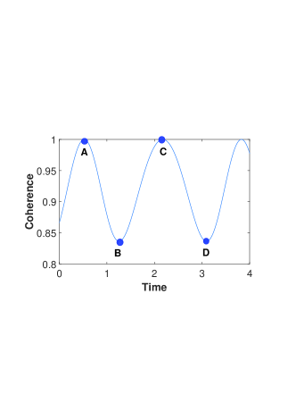
Supplementary Figure  1: The points $A$, $B$, $C$ and $D$ are four extreme points within one period. Note that in the $\mathcal{PT}$-symmetric-unbroken regime, there are two backflows of coherence inside a simple period of coherent evolution.

IX Proof for the characteristics of backflow in the $\mathcal{APT}$-symmetric-unbroken regime

For an arbitrary initial state $|\phi\rangle=\alpha|H\rangle+\beta e^{i\varphi}|V\rangle$, the coherence of the evolved state in the $\mathcal{APT}$-symmetric systems is given by Eq. (S31). In the $\mathcal{APT}$-symmetric-unbroken regime (i.e., $a>1$), $A$, $B$ and $C$ are given by Eq. (S26). In view of Eq. (S32), the derivative of $C_{l_{1}}\left(|\phi(t)\rangle\right)$ can be expressed as:

$$\frac{dC_{l_{1}}\left(|\phi(t)\rangle\right)}{dt}=\frac{dC_{l_{1}}\left(|\phi(t)\rangle\right)}{dm_{3}}\times\frac{dm_{3}}{d\theta_{3}}\times\frac{d\theta_{3}}{dt}.$$ (S50)

Note that $\frac{d\theta_{3}}{dt}=\omega_{3}s>0$. Thus, to meet $\frac{dC_{l_{1}}\left(|\phi(t)\rangle\right)}{dt}=0$, it follows from Eq. (S50):

$$\frac{dC_{l_{1}}\left(|\phi(t)\rangle\right)}{dm_{3}}=0,$$ (S51)

or

$$\frac{dm_{3}}{d\theta_{3}}=0.$$ (S52)

First, we consider the case when $\frac{dC_{l_{1}}\left(|\phi(t)\rangle\right)}{dm_{3}}=0$. According to Eq. (S32), we have

$$\frac{dC_{l_{1}}\left(|\phi(t)\rangle\right)}{dm_{3}}=\frac{1-m_{3}}{(1+m_{3})^{2}\sqrt{m_{3}}}=0.$$ (S53)

Because of $m_{3}=x_{3}/y_{3}$ and according to Eq. (S33), we have

$$m_{3}=\frac{\left[\omega_{3}^{2}\alpha^{2}+\alpha\beta\omega_{3}\cos\varphi\sin 2\theta_{3}+\frac{1-\cos 2\theta_{3}}{2}\left(1-a\alpha\beta\sin\varphi\right)\right]}{\left[\omega_{3}^{2}\beta^{2}+\alpha\beta\omega_{3}\cos\varphi\sin 2\theta_{3}+\frac{1-\cos 2\theta_{3}}{2}\left(1-a\alpha\beta\sin\varphi\right)\right]}.$$ (S54)

Substituting Eq. (S54) into Eq. (S53) leads to

$$\alpha^{2}-\beta^{2}=0.$$ (S55)

In general, Eq. (S55) is not satisfied for an arbitrary initial state $\alpha|H\rangle+\beta e^{i\varphi}|V\rangle$.

Now, we consider the other case of $dm_{3}/d\theta_{3}=0$. Because of $m_{3}=x_{3}/y_{3}$ and according to Eq. (S33), one has

$$\frac{dm_{3}}{d\theta_{3}}=\frac{x_{3}^{\prime}y_{3}-x_{3}y_{3}^{\prime}}{y_{3}^{2}},$$ (S56)

where

$$x_{3}^{\prime}=\frac{1}{\omega_{3}^{2}}\left[2\alpha\beta\omega_{3}\cos\varphi\cos 2\theta_{3}+\sin 2\theta_{3}\left(1-a\alpha\beta\sin\varphi\right)\right],$$

$$y_{3}^{\prime}=\frac{1}{\omega_{3}^{2}}\left[2\alpha\beta\omega_{3}\cos\varphi\cos 2\theta_{3}+\sin 2\theta_{3}\left(1-a\alpha\beta\sin\varphi\right)\right].$$ (S57)

According to Eqs. (S33, S56, S57), one can easily find that the condition for $dm_{1}/d\theta_{1}=0$ is:

$$\tan 2\theta_{3}=-\frac{2\alpha\beta\omega_{3}\cos\varphi}{1-a\alpha\beta\sin\varphi}.$$ (S58)

Because the period of $\tan 2\theta_{3}$ is $\frac{\pi}{2}$ and the period of $C_{l_{1}}\left(|\phi(t)\rangle\right)$ is $T_{\theta_{3}}$=$\pi$ (i.e., $T_{\mathcal{APT}}$=$\frac{\pi}{s\sqrt{a^{2}-1}}$), one period of $C_{l_{1}}\left(|\phi(t)\rangle\right)$ includes two periods of $\tan 2\theta_{3}$. Thus, there exist two different values of $\theta_{3}$ (or $t$) satisfying Eq. (S58) or Eq. (S52) within one period of $C_{l_{1}}\left(|\phi(t)\rangle\right)$.

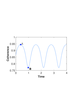
Supplementary Figure  2: The points $A$ and $B$ are two extreme points in one period. The coherent oscillation of quantum states in the $\mathcal{APT}$-symmetric-unbroken regime has only one backflow within one period.

From the above discussion, one can conclude that $\frac{dC_{l_{1}}\left(|\phi(t)\rangle\right)}{dt}$ has two zero points in one period (i.e., $T_{\mathcal{APT}}$=$\frac{\pi}{s\sqrt{a^{2}-1}}$) of coherent evolution. Therefore, the coherent oscillation of quantum states in the $\mathcal{APT}$-symmetric-unbroken regime has only one backflow within one period (eg., see Supplementary Figure 2).

X Experimental implementation of the loss operator $L$

As illustrated in Supplementary Figure 3, we experimentally implement the loss operator $L$ by a combination of two beam displacers ($\rm BD_{1}$ and $\rm BD_{2}$) and two half-wave plates ($\rm HWP_{1}$ and $\rm HWP_{2}$). Here, the optical axes of the BDs are cut so that the vertically polarized photons are transmitted directly, while the horizontally polarized photons are displaced into the lower path. In addition, the $\rm HWP_{1}$ and $\rm HWP_{2}$ with setting angles $\xi_{i}$ and $\xi_{j}$ are, respectively, inserted into the upper and lower paths between the two BDs. The rotation operations on the photon polarization states, performed by the $\rm HWP_{1}$ and $\rm HWP_{2}$, are given as follows:

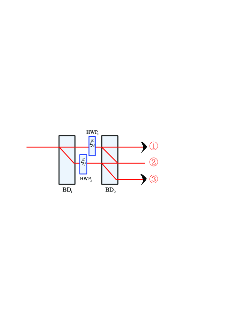
Supplementary Figure  3: Experimental setup to realize a loss operator, where $\xi_{i}$ and $\xi_{j}$ are the two tunable setting angles for the half-wave plates $\rm HWP_{1}$ and $\rm HWP_{2}$, respectively.

$$R_{\rm HWP}\left(\xi_{i}\right)=\left(\begin{array}[]{cc}\cos 2\xi_{i}&\sin 2\xi_{i}\\ \sin 2\xi_{i}&-\cos 2\xi_{i}\\ \end{array}\right),~{}~{}~{}~{}R_{\rm HWP}\left(\xi_{j}\right)=\left(\begin{array}[]{cc}\cos 2\xi_{j}&\sin 2\xi_{j}\\ \sin 2\xi_{j}&-\cos 2\xi_{j}\\ \end{array}\right).$$ (S59)

In this case, when a horizontally polarized photon passes through the experimental setup, one can find that

$$|H\rangle~{}\xrightarrow{\rm BD_{1}}~{}|H\rangle_{\rm lower}~{}\xrightarrow{R_{\rm HWP}(\xi_{j})}~{}R_{\rm HWP}(\xi_{j})|H\rangle~{}\xrightarrow{\rm BD_{2}}~{}\cos 2\xi_{j}|H\rangle_{3}+\sin 2\xi_{j}|V\rangle_{2},$$ (S60)

where the subscript “lower” represents the lower path between the two BDs, while subscripts “2” and “3” represent the two paths $2$ and $3$ after the second BD, respectively. Similarly, when a vertically polarized photon pass the experimental setup, one can find that

$$|V\rangle~{}\xrightarrow{\rm BD_{1}}~{}|H\rangle_{\rm upper}~{}\xrightarrow{R_{\rm HWP}(\xi_{i})}~{}R_{\rm HWP}(\xi_{i})|V\rangle~{}\xrightarrow{\rm BD_{2}}~{}\sin 2\xi_{i}|H\rangle_{2}-\cos 2\xi_{i}|V\rangle_{1},$$ (S61)

where the subscript “upper” represents the upper path between the two BDs, while subscripts “1” and “2” represent the two paths $1$ and $2$ after the second BD, respectively. That is, only horizontally polarized photons in the upper path and vertically polarized photons in the lower path are transmitted through the second BD and then combined onto path $2$, while the other photons transmitted onto path $1$ or $3$ are blocked, i.e., they are discarded and lost from the system.

In this sense, according to Eqs. (S60) and (S61), when the input photon is initially in the state $|\phi\rangle_{\rm in}=\alpha|H\rangle+\beta e^{i\varphi}|V\rangle$, then the output photon appearing in the path $2$ would be in the state $|\phi\rangle_{\rm out}=\alpha\sin 2\xi_{j}|V\rangle_{2}+\beta e^{i\varphi}\sin 2\xi_{i}|H\rangle_{2}$. It is obvious that this state transformation can be written as $|\phi\rangle_{\rm out}=L|\phi\rangle_{\rm in}$, with a polarization-dependent photon loss operator $L$, given by

$$L\left(\xi_{i},~{}\xi_{j}\right)=\left(\begin{array}[]{cc}0&\sin 2\xi_{i}\\ \sin 2\xi_{j}&0\\ \end{array}\right),$$ (S62)

where $\xi_{i}$ and $\xi_{j}$ are, respectively, the two tunable setting angles for the half-wave plates $\rm HWP_{1}$ and $\rm HWP_{2}$ (Supplementary Figure 3).

XI Coherence flow for two-qubit $\mathcal{PT}$- and anti-$\mathcal{PT}$- symmetric systems

We have numerically simulated the dynamics of coherence for two-qubit $\mathcal{PT}$/$\mathcal{APT}$ systems. As shown in Supplementary Figures 4(a, c), there exist different periodic oscillations of coherence (including one coherence backflow, two coherence backflows, and multiple coherence backflows in one period) for $\mathcal{PT}$/$\mathcal{APT}$-symmetric systems in the unbroken regime. In addition, as illustrated in Supplementary Figures 4(b, d), there exists PSV for both $\mathcal{PT}$ -and $\mathcal{APT}$ -symmetric systems in the broken regime, which are independent of the initial states.

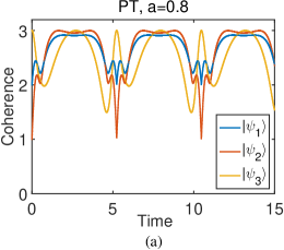
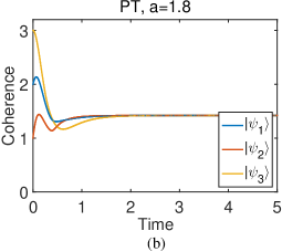
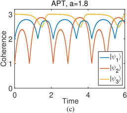
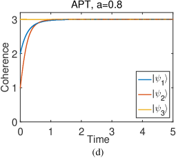
Supplementary Figure  4: The evolution of coherence for three different initial states in a two-qubit $P\mathcal{T}$ /$\mathcal{APT}$ -symmetric system. We consider the two qubits undergoing the same $\mathcal{PT}$/$\mathcal{APT}$ -symmetric dynamic process, i.e., the parameters $a$ involved in the Hamiltonians (1) and (2) of the main text are set to be the same for both qubits. (a) $a=0.8$, the $\mathcal{PT}$ symmetry unbroken regime; (b) $a=1.8$, the $\mathcal{PT}$ symmetry broken regime; (c) $a=1.8$, the $\mathcal{APT}$ symmetry unbroken regime; (d) $a=0.8$, the $\mathcal{APT}$ symmetry broken regime. The three initial states are $|\psi_{1}\rangle=\frac{1}{\sqrt{3}}\left(|00\rangle+|01\rangle+|11\rangle\right)$ (blue curves), $|\psi_{2}\rangle=\frac{1}{\sqrt{2}}\left(|00\rangle+e^{i\pi/5}|11\rangle\right)$ (red curves), and $|\psi_{3}\rangle=\frac{1}{2}\left(|00\rangle+|01\rangle+|10\rangle+e^{i\pi/5}|11\rangle\right)$ (yellow curves).